Third-Order Sliding Mode Control for Trajectory Tracking of Quadcopters Using Particle Swarm Optimization

Abstract

This study focuses on designing a controller for trajectory tracking of quadcopters using advanced sliding-mode techniques. Specifically, an integral terminal sliding-mode control based on an adaptive barrier function with a super-twisting reaching law is employed to achieve precise trajectory tracking. The performance of the controller is enhanced by applying Particle Swarm Optimization to fine-tune the gain values. The nonlinear dynamics of the quadcopter are modeled using the Euler–Lagrange approach, followed by a Lyapunov stability analysis to verify the stability of the controller. The adaptive barrier function is used to prevent control signal saturation, while the third-order sliding-mode controller effectively reduces the chattering. Additionally, a saturation function is introduced to further mitigate the chattering effect. The effectiveness of the proposed approach is demonstrated through numerical simulations, and its performance is further validated through controller-in-the-loop implementation. The results show that the proposed method significantly improves trajectory-tracking accuracy.

1. Introduction

The trajectory tracking of quadcopters remains a significant challenge due to their underactuated nature and complex dynamics. Researchers are increasingly focusing on designing controllers that can effectively manage these complexities to improve trajectory-tracking performance. Despite the challenges of underactuated systems, the simplified configurations, energy efficiency, agility, and versatility of quadcopters make them essential in various applications such as education [1], mapping and data collection [2,3], search and rescue operations [4,5], agricultural practices [6,7], military operations [8], and disaster response [9,10]. The widespread interest in quadcopters within the UAV research domain is driven by their simple design, ease of operation, robustness, and compact size. However, the nonlinear dynamics of quadcopters, influenced by aerodynamics, complicate the development of accurate trajectory-tracking control.

To address the trajectory-tracking control of quadcopter drones, various control techniques have been explored by researchers, each aiming to enhance performance and robustness in dynamic environments. For instance, in [11], the authors implemented a PID-based control scheme to regulate both the altitude and attitude of the quadrotor. A more advanced approach is presented in [12], where a quaternion-based tracking controller, utilizing the pseudo-linear feedback linearization method, was proposed for the attitude and altitude regulation of quadrotor drones. In another study, ref. [13] introduced physics-informed neural networks for estimating UAV dynamic models, effectively addressing uncertain data, non-linearities, and noise. Once trained, their neural network provides robust control with fast computation, eliminating the need for retraining. Furthermore, in [14], the authors proposed an image-based visual servoing control structure for UAV target tracking, combining a sliding-mode controller for tracking and disturbance rejection with a controller to correct velocity errors due to UAV dynamics.

Among the various strategies, the sliding-mode control (SMC) technique has gained prominence for controlling the nonlinear dynamics of quadcopter drones, making it a common choice in the literature. Numerous studies have applied SMC and its advanced variants to address the challenges of quadcopter control. In [15], the authors developed a sliding-mode control approach based on the backstepping method, effectively handling high-order nonholonomic constraints and incorporating essential physical phenomena into the dynamic model of a quadcopter. To further enhance SMC, ref. [16] proposed an integrated control strategy, combining integral SMC and backstepping SMC within a dual-loop framework, which significantly improved trajectory-tracking accuracy. In continuation of this, ref. [17] demonstrated the efficacy of nonlinear adaptive control through a modified adaptive SMC strategy, particularly for mini-drone quadcopters. Additionally, ref. [18] introduced an integral adaptive SMC scheme, which ensured robustness against nonlinear dynamics and external disturbances. Further advancements were made by [19], who integrated an adaptive super-twisting integral terminal sliding-mode control with a barrier function to address quadcopter attitude and altitude challenges. This approach was refined in [20] with a conditioned adaptive barrier-based double-integral super-twisting SMC designed to ensure robust trajectory tracking. To further improve trajectory tracking, ref. [21] employed a double-integral SMC approach, while ref. [22] introduced an adaptive SMC strategy with an adaptive switching gain to achieve rapid response against parameter uncertainties and disturbances. In [23], the authors addressed mass and inertia uncertainties using adaptive laws to compensate for input saturation, incorporating a disturbance observer to counter external disturbances. In another study [24], the authors proposed a sliding-mode controller for quadrotor attitude, integrating adaptive fuzzy gain scheduling to mitigate chattering, along with a PD controller for position control. Similarly, in [25], the authors introduced an adaptive distributed sliding-mode control strategy with a prescribed performance function, ensuring both transient and steady-state performance.

In addition, several researchers have explored various second-order and third-order sliding-mode control methods to further enhance the performance of quadcopters. For instance, ref. [26] developed a second-order sliding-mode control incorporating nonholonomic constraints and employed a sigmoid function to reduce chattering, effectively addressing position and attitude tracking challenges, while ref. [27] improved it by integrating the super-twisting algorithm, enhancing tracking accuracy. Further advancements include the work of [28], who introduced an adaptive proportional-integral-derivative-based SMC strategy to stabilize the attitude and position of quadrotor UAVs amid parameter uncertainties and external disturbances. Similarly, ref. [29] presented a robust adaptive second-order sliding-mode controller to enhance tracking performance for both attitude and altitude under such disturbances and uncertainties. In parallel, ref. [30] proposed a super-twisting algorithm-based second-order SMC method for trajectory tracking and ref. [31] introduced an improved adaptive sliding-mode control framework that integrates an adaptive switching gain for rapid adaptation and robustness against external disturbances. Moreover, third-order sliding-mode control has been applied to various engineering domains. Notably, ref. [32] proposed a novel adaptive integral terminal third-order sliding-mode control strategy for motion tracking in piezoelectric-driven nano-positioning systems, while ref. [33] utilized a third-order sliding-mode control based on a super-twisting algorithm for trajectory tracking in quadcopters. These contributions collectively demonstrate the ongoing development and versatility of sliding-mode control techniques in addressing complex control challenges, particularly in the context of quadcopter trajectory tracking.

Furthermore, recent studies have widely applied fractional-order sliding-mode control (FOSMC) techniques to enhance the performance of quadrotor systems. For instance, in [34], the authors proposed a FOSMC method specifically designed for fractional-order quadrotor systems, aiming to improve system stability and control accuracy. Similarly, in [35], a fractional-order sliding-mode control approach was introduced to address disturbances in quadrotor systems, just as in [36], where the author designed a proportional-derivative sliding-mode controller specifically to handle disturbances in a quadrotor system. This approach incorporates an adaptive strategy to estimate disturbance bounds, which significantly contributes to the robustness of the system. Additionally, in [37], a robust fractional-order sliding-mode control method was developed for quadrotor tracking under external disturbances, with the added objective of stabilizing the attached slung load system.

Additionally, several surveys have been conducted on control strategies for quadcopters, as detailed in [38], providing an overview of various approaches implemented for system control. Among these, sliding-mode control (SMC) techniques have gained significant attention, particularly for trajectory tracking, where they have proven effective in rejecting disturbances. While SMC has been successfully applied to path following in fixed-wing UAVs, its application in quadrotor path following remains largely unexplored. Another survey by the authors in [39] discusses recent advancements in motion control theory for multi-rotor aerial vehicles (MAVs), focusing on position and attitude control. The survey reviews control strategies for MAVs, emphasizing the importance of position and attitude controllers in ensuring stability and achieving desired movement. The authors highlight sliding-mode control as a widely researched nonlinear control method known for managing system dynamics using a discontinuous control signal that forces the system to “slide” along a trajectory. Initially proposed for attitude control, SMC has since been applied to position control, with real-world validation occurring in the past decade.

While the sliding-mode control approach is widely recognized for addressing the control challenges of quadcopters, certain aspects of the existing literature present opportunities for further enhancement. For example, several studies, including [20,22,23,30,31,40], employed a PD-based function to select the sliding surface, which may limit the controller flexibility. Additionally, works such as [15,16,23] have developed SMC controllers without thoroughly addressing the chattering phenomenon, which could potentially impact performance under specific operational conditions. Moreover, studies such as [15,16,21,30,31] show that there exists potential for further exploration in optimizing the gain parameters, which could lead to a more robust and efficient system performance. Furthermore, research including [19,20,23] has addressed the issue of control signal saturation, an area that still presents opportunities for further investigation to enhance the performance of the controller under specific constraints. Furthermore, many of these studies primarily focus on simulation-based evaluations, with only a few, such as [20,40,41], demonstrating their implementations on physical hardware or through hardware-in-the-loop (HIL) testing. This highlights valuable opportunities for advancing the design, optimization, and real-world application of quadcopter control systems.

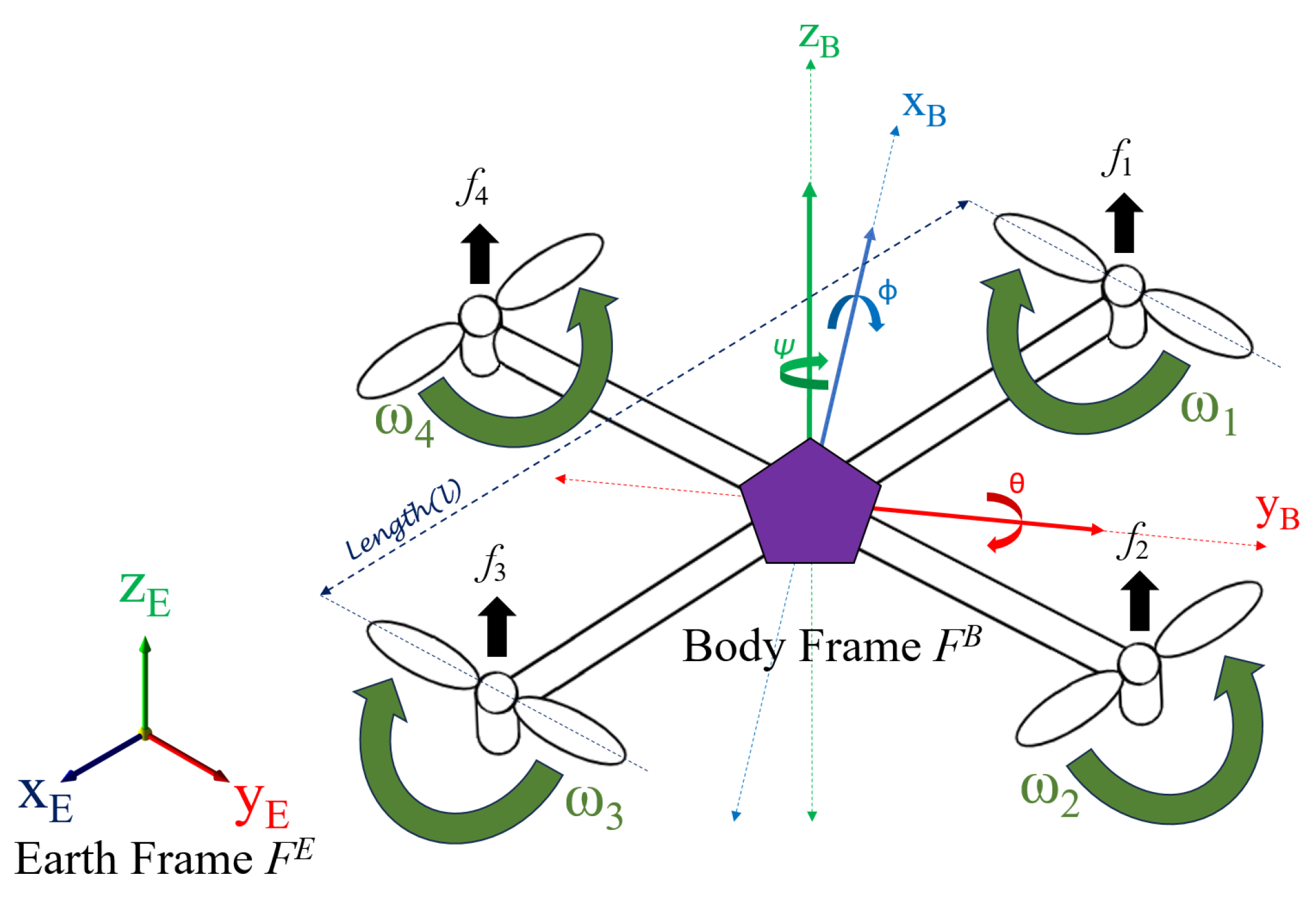
In this study, we investigate the trajectory-tracking control problem of a quadcopter and design a controller to regulate its attitude, heading, position, and altitude. The cross configuration of the quadcopter is selected for its superior maneuverability. To enhance the robustness of traditional sliding-mode control (SMC), a third-order sliding-mode controller is used, incorporating a two-stage dynamic sliding surface. This approach is particularly effective for nonlinear systems, as it offers a flexible method for handling complex dynamics. In contrast, ref. [20] employs a simpler, single-stage sliding surface, where a PD sliding surface is used. Additionally, a barrier function is integrated to regulate excessive gain and ensure convergence to the origin. The integral terminal sliding-mode technique, in conjunction with the super-twisting reaching law, is used to mitigate chattering effects. To ensure continuous control actions, enable smoother transitions, and minimize chattering, a saturation function is used instead of the traditional signum function, as implemented in [20]. Additionally, Particle Swarm Optimization (PSO) is used to fine-tune the controller’s gain parameters, with Integral Time Absolute Error (ITAE) as the objective function. In contrast to [20], which uses Improved Grey Wolf Optimization (IGWO) with Integral Square Error (ISE) as the objective function, PSO with ITAE effectively minimizes both transient and steady-state errors. While ISE primarily focuses on steady-state error, it may not capture transient dynamics as effectively as ITAE.

Optimization of control strategies and the overall system is crucial for achieving optimal performance. To enhance controller performance, various optimization techniques have been employed by researchers. For instance, in [20], an Improved Grey Wolf Optimization technique was used to fine-tune the gain parameters of the controller. In contrast, ref. [36] employed a genetic algorithm for tuning the parameters of the controller. Meanwhile, ref. [41] used the Redfox algorithm for the same purpose. Among the numerous optimization methods, Particle Swarm Optimization (PSO) is particularly favored for its versatility and robustness. As highlighted in [42], PSO has been successfully applied in chemometrics for tasks such as metaparameter selection, signal warping, robust PCA, and variable selection. Similarly, ref. [43] explored PSO as a robust solution for large-scale nonlinear problems and its applications in power systems. In [44,45], PSO was employed to optimize controller gain values. Additionally, in [46], PSO was combined with an enumeration method to derive candidate chassis layout schemes for Unmanned Surface Vehicles, showcasing its adaptability across various engineering fields. Further applications of PSO include [47], where enhanced PSO methods were applied for UAV localization in GPS-denied environments. These studies highlight the diversity of optimization techniques, with PSO standing out as a powerful tool for enhancing control system performance and efficiency.

The primary limitations of SMC-based control laws include high control gains, increased computational load, chattering effects, and control input saturation. However, these limitations can be alleviated through the utilization of advanced SMC techniques. In this study, we implement a third-order SMC approach to address the trajectory-tracking control problem, utilizing the cross configuration of the quadcopter. The key contributions of this research are as follows:

• The control input is regulated near the sliding surface through the integral terminal super-twisting technique, mitigating chattering and enhancing control performance.
• Dynamic selection of the sliding surface is utilized to optimize the performance of the control algorithm.
• The barrier function regulates excessive gain, improves control performance and increases robustness by protecting the system from uncertainties.
• The barrier function effectively adapts to variations in time-varying systems.
• The saturation function promotes smoother transitions and helps reduce chattering.
• Particle Swarm Optimization is employed to optimize the gain parameters, further improving the overall performance of the controller.

Table 1. Comparative Analysis of SMC Strategies and Parameter Selection for Quadcopter Systems.

Control Technique	Sliding Surface Criteria	Control Signal Saturation	Optimization Technique	Method for Chattering Reduction	Control Problem
Adaptive Super-Twisting SMC [40]	PD	X	Adaptive	Super-Twisting	Position and Attitude
Adaptive PID using SMC [28]	PID	X	Gradient and Chain Rule	Fuzzy Compensator	Attitude and Position
Adaptive Sliding-Mode Controller [22]	PD	X	Adaptive	Approximation of sign Function	External and Internal Loops
CABDIST-SMC [20]	PD	✓	Improved Grey Wolf Optimization	Barrier Function and Double Integral	Trajectory Tracking
Double-Integral SMC [21]	PII	X	X	Double Integral	Attitude and Altitude
Second-order SMC [31]	PD	X	X	Second-order SMC	External and Internal Loops
SMC based on Backstepping [15]	PD with Backstepping	X	X	X	Trajectory Tracking
Backstepping Sliding-Mode Control [16]	P with Backstepping and PID	X	X	X	Attitude and Position
Barrier-Based Adaptive Super-Twisting Integral Terminal SMC [19]	PID	✓	Adaptive	Super-Twisting	Attitude and Altitude
Adaptive SMC [23]	PD	✓	Adaptive	X	Trajectory Tracking
Adaptive Second-Order SMC [29]	PID	X	Adaptive	Sat Function	Attitude and Altitude
Second-Order SMC [30]	PD	X	X	Super-Twisting	Trajectory Tracking
Proportional-Derivative SMC [36]	PD	X	Genetic Algorithm	Sigmoidal function	Trajectory Tracking
Fractional Order SMC [34]	PD with Fractional Order	X	X	Fractional Order	Trajectory Tracking
Robust Fractional Order SMC [37]	PD with Fractional Order	X	X	Fractional Order	Altitude and Attitude
Proposed SMC	PID with Integral Terminal	✓	Particle Swarm Optimization	Sat Function and Super-Twisting	Trajectory Tracking

provides a comparative summary of the proposed approach and existing methods, highlighting the key differences.

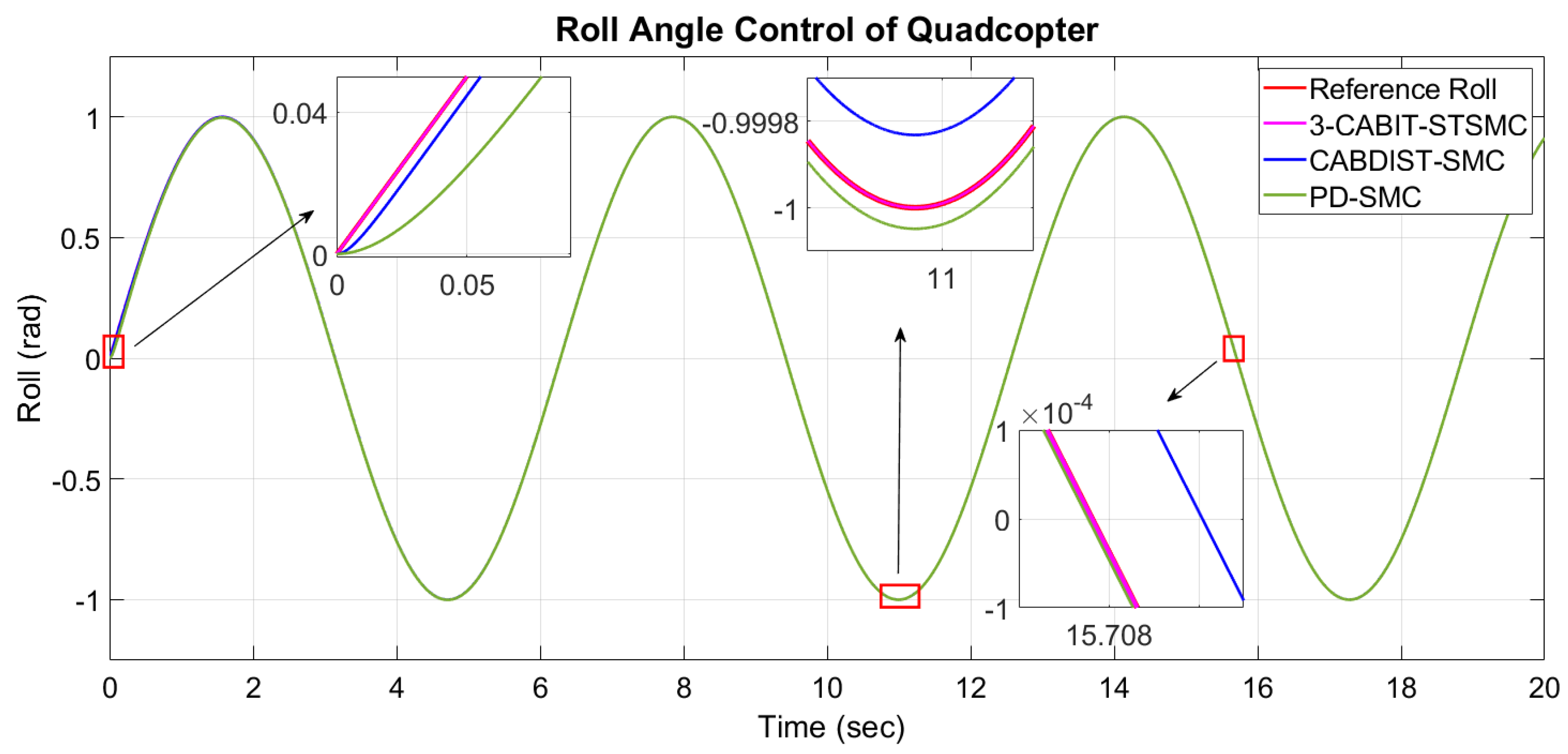
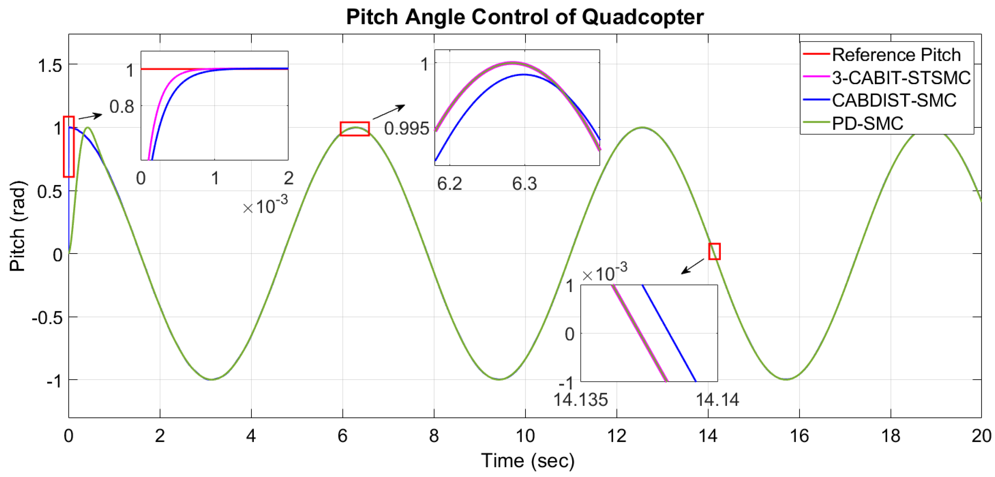
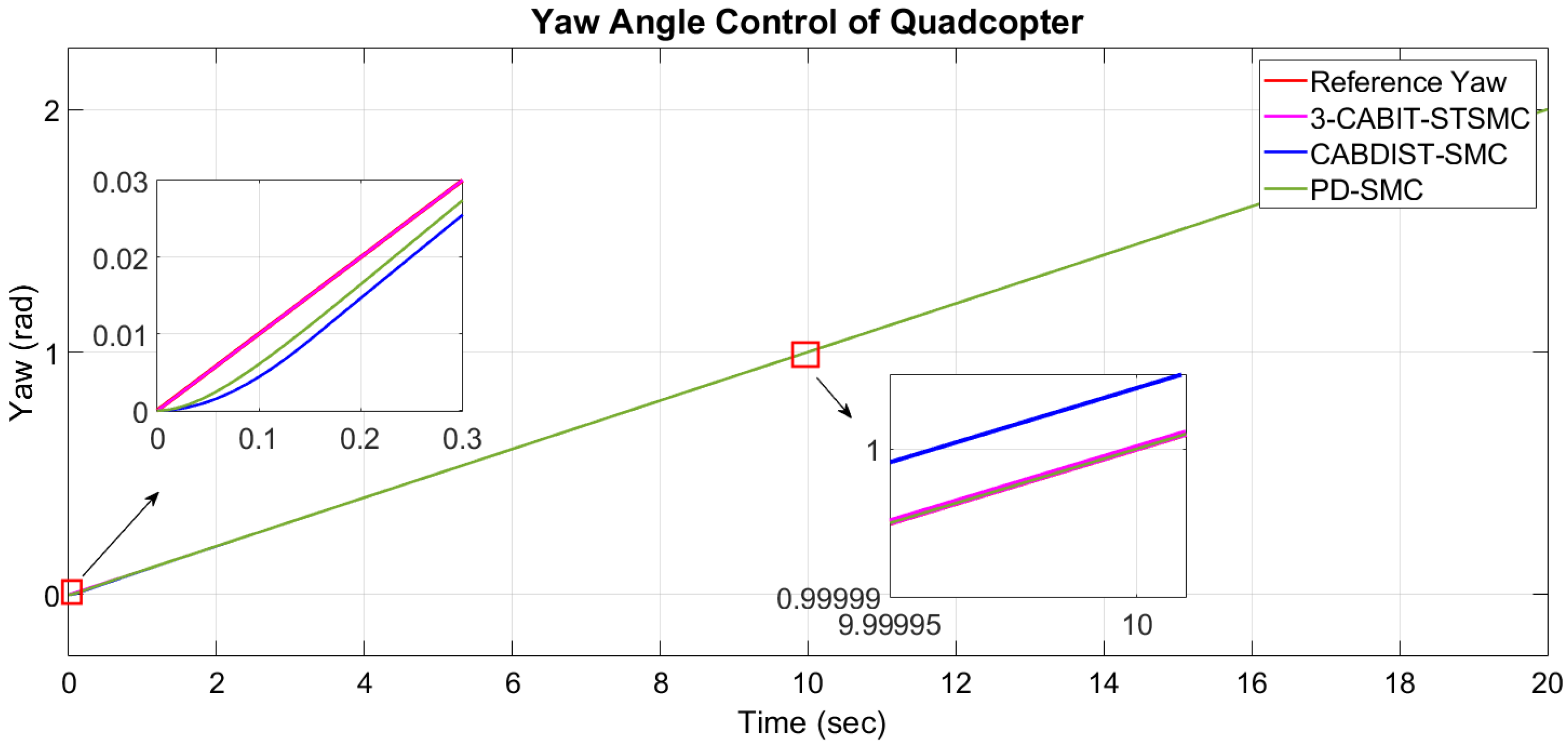
This article is organized as follows: Section 2 introduces the dynamic mathematical model for the quadcopter. Section 3 describes the design of the third-order sliding-mode control technique, including the optimization of controller gain parameters through Particle Swarm Optimization. In Section 4, the numerical simulation results are presented, followed by a comparative analysis of control laws in Section 5. Section 6 outlines the implementation of the controller-in-the-loop experiment, and Section 7 provides the concluding remarks of the study.

2. Mathematical Modeling of Quadcopter

This section presents the development of the mathematical model for the quadcopter system using the Lagrangian approach. Numerous studies have investigated the modeling and design of quadcopters with various configurations, including the cross configuration (X-shape), plus-shape, and H-shape, each characterized by distinct dynamic models, aerodynamic properties, and flight characteristics. Among these configurations, the cross configuration is widely recognized for its superior stability and maneuverability, as highlighted in [11], with further modeling advancements discussed in [17,28,40]. Additionally, the thrust dynamics and component-level modeling of quadcopters are analyzed in [48], while [15,49] focus on the dynamic modeling and experimental validation of the plus-shape configuration.

In this study, a cross configuration is selected, where all four motors contribute to the maneuverability of the quadcopter, offering superior stability compared to the conventional plus configuration. The system dynamics are described using two primary coordinate frames: the Earth frame ($F^E$), defined by the coordinates $x_E$, $y_E$, and $z_E$, and the body frame ($F^B$), represented by the axis $x_B$, $y_B$, and $z_B$, as illustrated in Figure 1. The quadcopter consists of four symmetric arms, each equipped with a motor and propeller. The thrust generated by each motor is directly proportional to the square of its angular velocity, which can be mathematically expressed as:

$$f_i\left(t\right)=K_p{\omega }_i^2\left(t\right)i=1,2,3,4$$

(1)

where $f_i\left(t\right)$ refers to the upward thrust force measured in N produced by the i -th motor, $K_p$ denotes the thrust constant in ${\mathrm{Ns}}^2{\mathrm{rad}}^{-2}$, and ${\omega }_i\left(t\right)$ indicates the angular velocity in ${\mathrm{rads}}^{-1}$. The movement of the quadcopter can be controlled by adjusting the angular velocities (${\omega }_1\left(t\right)$, ${\omega }_2\left(t\right)$, ${\omega }_3\left(t\right)$, and ${\omega }_4\left(t\right)$) of the motors. Additionally, the arm length is denoted as $\mathit{l}$ (in meters), and the gravitational force acts along the $z_E$ axis (in ${\mathrm{ms}}^{-2}$) as shown in Figure 1. Also, to minimize the net rotation, motors with angular velocities ${\omega }_1\left(t\right)$ and ${\omega }_3\left(t\right)$ rotate clockwise, while ${\omega }_2\left(t\right)$ and ${\omega }_4\left(t\right)$ rotate counterclockwise. This configuration enables both lift generation and maneuverability. The quadcopter system is inherently underactuated, requiring a model that incorporates certain simplifying assumptions for efficient control. These assumptions include:

• The structure is rigid.
• The system exhibits symmetry.
• The origin of the body frame coincides with the center of gravity.
• Blade flapping is neglected, and the propellers are assumed to be rigid.
• All propellers operate under identical conditions, with equal thrust and response torque coefficients.

These assumptions simplify the modeling of the quadcopter, thus facilitating the development of effective control strategies.

2.1. Quadcopter Kinematics

In this section, the kinematics of the quadcopter are explained, where the Earth frame ($F^E$) is used to describe the roll, pitch, and yaw angles, and the body frame ($F^B$) is employed to represent the linear velocities and accelerations. The quadcopter is characterized by six degrees of freedom (6-DOF), which are defined by its position coordinates ($x\left(t\right)$, $y\left(t\right)$, $z\left(t\right)$) and orientation angles ($\varphi \left(t\right)$, $\theta \left(t\right)$, $\psi \left(t\right)$), as shown in Figure 1. To provide a more comprehensive representation of the quadcopter states, these six degrees of freedom can be expressed as a single vector [27], as follows:

$$\mathcal{E}\left(\mathit{t}\right)={\left[\begin{array}{cccccc}x\left(t\right)& y\left(t\right)& z\left(t\right)& \varphi \left(t\right)& \theta \left(t\right)& \psi \left(t\right)\end{array}\right]}^T$$

(2)

Here, $\mathcal{E}\left(\mathit{t}\right)$ is the state vector, and its derivative $\dot{\mathcal{E}}\left(\mathit{t}\right)$ represents the generalized velocity vector, can be described in the body frame as:

$$\dot{\mathcal{E}}\left(\mathit{t}\right)=\mathbf{Jv}\left(t\right)$$

(3)

In this equation, $\mathbf{v}\left(t\right)$ represents the velocity vector, and $\mathbf{J}$ is the generalize matrix that incorporates both the rotation and transformation between frames. The velocity vector in the body frame is given by:

$$\mathbf{v}\left(t\right)={\left[\begin{array}{cc}{\mathbf{v}}^B\left(t\right)& {\mathsf{\omega }}^B\left(t\right)\end{array}\right]}^T={\left[\begin{array}{cccccc}{\mathrm{v}}_x\left(t\right)& {\mathrm{v}}_y\left(t\right)& {\mathrm{v}}_z\left(t\right)& {\omega }_x\left(t\right)& {\omega }_y\left(t\right)& {\omega }_z\left(t\right)\end{array}\right]}^T$$

(4)

where ${\mathrm{v}}_x\left(t\right),{\mathrm{v}}_y\left(t\right),{\mathrm{v}}_z\left(t\right)$ are the linear velocity components, and ${\omega }_x\left(t\right),{\omega }_y\left(t\right),{\omega }_z\left(t\right)$ are the angular velocity components. The generalized matrix $\mathbf{J}$ facilitates the conversion of velocities from the body frame to the inertial frame, described as:

$$\mathbf{J}=\left[\begin{array}{cc}\mathbf{R}& 0_{3\times 3}\\ 0_{3\times 3}& \mathbf{T}\end{array}\right]$$

(5)

Here, $\mathbf{R}$ is the rotation matrix, and $\mathbf{T}$ is the transformation matrix. The rotation matrix defines the orientation of the object. The rotation matrix based on Euler angles [27] is expressed as:

$$\mathbf{R}=\left[\begin{array}{ccc}{C}_{\psi }{C}_{\theta }& C_{\psi }{S}_{\theta }{S}_{\varphi }-S_{\psi }{C}_{\varphi }& C_{\psi }{S}_{\theta }{C}_{\varphi }+S_{\psi }{S}_{\varphi }\\ S_{\psi }{C}_{\theta }& S_{\psi }{S}_{\theta }{S}_{\varphi }+C_{\psi }{C}_{\varphi }& S_{\psi }{S}_{\theta }{C}_{\varphi }-C_{\psi }{S}_{\varphi }\\ -S_{\theta }& C_{\theta }{S}_{\varphi }& C_{\psi }{C}_{\theta }\end{array}\right]$$

(6)

where $C_{\varphi }=cos\left(\varphi \right),C_{\theta }=cos\left(\theta \right),C_{\psi }=cos\left(\psi \right),S_{\varphi }=sin\left(\varphi \right),S_{\theta }=sin\left(\theta \right)$ and $S_{\psi }=sin\left(\psi \right)$. The rotation matrix $\mathbf{R}$ represents the transformation between coordinate frames, and it is orthogonal, satisfying the property ${\mathbf{R}}^{-1}={\mathbf{R}}^T$. Typically, angles and angular velocities are measured in the inertial frame ($F^E$), and the transformation matrix $\mathbf{T}$ is used to map angular velocities from the body-fixed frame ($F^B$) to $F^E$.

$$\mathbf{T}=\left[\begin{array}{ccc}1& S_{\varphi }{T}_{\theta }& C_{\varphi }{T}_{\theta }\\ 0& C_{\varphi }& -S_{\varphi }\\ 0& S_{\varphi }/C_{\theta }& C_{\varphi }/C_{\theta }\end{array}\right]$$

(7)

where $T_{\theta }=tan\left(\theta \right)$. The inverse transformation matrix ${\mathbf{T}}^{-1}$ is used to convert angular velocities from the inertial frame to the body frame.

2.2. Quadcopter Dynamics

In this section, the dynamics of a six-degrees-of-freedom (6-DOF) quadcopter are described, taking into account its mass (m) and inertia ($\mathbf{I}$). The quadcopter frame is assumed to be symmetric, with the propellers aligned along the x and y axis. As explained in [11], the inertia matrix is diagonal. The dynamics of the quadcopter, expressed in terms of linear and angular forces, can be formulated as:

$$\left[\begin{array}{c}{\mathit{f}}^B\left(t\right)\\ {\mathsf{\tau }}^B\left(t\right)\end{array}\right]=\left[\begin{array}{c}m{\dot{\mathbf{v}}}^B\left(t\right)+{\mathsf{\omega }}^B\left(t\right)\times \left(m{\mathbf{v}}^B\left(t\right)\right)\\ \mathbf{I}{\dot{\mathsf{\omega }}}^B\left(t\right)+{\mathsf{\omega }}^B\left(t\right)\times \left(\mathbf{I}{\mathsf{\omega }}^B\left(t\right)\right)\end{array}\right]$$

(8)

Here, ${\dot{\mathbf{v}}}^B\left(t\right)$ denotes linear acceleration, ${\dot{\mathsf{\omega }}}^B\left(t\right)$ represents angular acceleration, ${\mathit{f}}^B\left(t\right)$ signifies linear force, and ${\mathsf{\tau }}^B\left(t\right)$ indicates torque, all defined in the body frame $F^B$. The quadcopter executes four primary maneuvers: thrust ($F_z\left(t\right)$), roll (${\tau }_{\varphi }\left(t\right)$), pitch (${\tau }_{\theta }\left(t\right)$), and yaw (${\tau }_{\psi }\left(t\right)$), each contributing to its overall motion as explained in [17].

The fundamental maneuvers of the quadcopter are controlled by four inputs, $u_1\left(t\right)$, $u_2\left(t\right)$, $u_3\left(t\right)$, and $u_4\left(t\right)$, which represent thrust, roll, pitch, and yaw control, respectively. Based on these inputs, Equation (8) can be reformulated as follows:

$$\left[\begin{array}{c}{\mathit{f}}^B\left(t\right)\\ {\mathsf{\tau }}^B\left(t\right)\end{array}\right]=\left[\begin{array}{c}0\\ 0\\ F_z\left(t\right)\\ {\tau }_{\varphi }\left(t\right)\\ {\tau }_{\theta }\left(t\right)\\ {\tau }_{\psi }\left(t\right)\end{array}\right]=\left[\begin{array}{c}0\\ 0\\ u_1\left(t\right)\\ u_2\left(t\right)\\ u_3\left(t\right)\\ u_4\left(t\right)\end{array}\right]=\left[\begin{array}{c}0\\ 0\\ K_p({\omega }_1^2\left(t\right)+{\omega }_2^2\left(t\right)+{\omega }_3^2\left(t\right)+{\omega }_4^2\left(t\right))\\ K_p{\displaystyle \frac{l}{2}}({\omega }_1^2\left(t\right)+{\omega }_2^2\left(t\right)-{\omega }_3^2\left(t\right)-{\omega }_4^2\left(t\right))\\ K_p{\displaystyle \frac{l}{2}}({\omega }_1^2\left(t\right)-{\omega }_2^2\left(t\right)-{\omega }_3^2\left(t\right)+{\omega }_4^2\left(t\right))\\ K_d({\omega }_1^2\left(t\right)-{\omega }_2^2\left(t\right)+{\omega }_3^2\left(t\right)-{\omega }_4^2\left(t\right))\end{array}\right]$$

(9)

where $K_p$ is the lift coefficient, $l/2$ is the distance from the center of gravity to the propeller axis, and $K_d$ is the drag coefficient.

As the motors are aligned horizontally, they generate vertical force $F_z\left(t\right)$ but do not directly produce forces in the x or y directions. However, movements along these axes can be controlled indirectly through the combination of the forces and torques generated by the motors. During the maneuvering of the quadcopter, both the kinetic energy ($T_{K.E}\left(q\left(t\right)\right)$) and potential energy ($T_{P.E}\left(q\left(t\right)\right)$) depend on the state of its coordinates, $q_i\left(t\right)=\{x\left(t\right),y\left(t\right),z\left(t\right),\varphi \left(t\right),$$\theta \left(t\right),\psi \left(t\right)\}$, which describe its position and orientation over time. These energies are defined by the following equations:

$$T_{K.E}\left(q\left(t\right)\right)={\displaystyle \frac{1}{2}}m({\mathrm{v}}_x^2\left(t\right)+{\mathrm{v}}_y^2\left(t\right)+{\mathrm{v}}_z^2\left(t\right))+{\displaystyle \frac{1}{2}}(I_x{\omega }_x^2\left(t\right)+I_y{\omega }_y^2\left(t\right)+I_z{\omega }_z^2\left(t\right))$$

(10)

$$T_{P.E}\left(q\left(t\right)\right)=mgz\left(t\right)$$

(11)

Here, g is the gravitational acceleration and $z\left(t\right)$ is the altitude. The Lagrangian function $\mathcal{L}\left(q\right(t\left)\right)$, defined as $\mathcal{L}\left(\mathit{q}\left(\mathit{t}\right)\right)=T_{K.E}\left(q\left(t\right)\right)-T_{P.E}\left(q\left(t\right)\right)$ combines the kinetic and potential energies. The equations of motion are derived using the Euler–Lagrange equation, which can be expressed as:

$${\displaystyle \frac{d}{dt}}\left({\displaystyle \frac{\partial \mathcal{L}\left(\mathit{q}\right(\mathit{t}\left)\right)}{\partial {\dot{\mathit{q}}}_i\left(t\right)}}\right)-{\displaystyle \frac{\partial \mathcal{L}\left(\mathit{q}\right(\mathit{t}\left)\right)}{\partial {\mathit{q}}_{\mathit{i}}\left(\mathit{t}\right)}}={\mathsf{\Gamma }}_i\left(t\right)i=1,2,\dots 6$$

(12)

where ${\mathsf{\Gamma }}_i\left(t\right)$ is the generalized force vector, with coordinates $q_i\left(t\right)=\{x\left(t\right),y\left(t\right),z\left(t\right),\varphi \left(t\right),$$\theta \left(t\right),\psi \left(t\right)\}$. The generalized force vector can be defined as:

$${\mathsf{\Gamma }}_i\left(t\right)=\left[\begin{array}{c}{\mathit{F}}_{ext}\left(t\right)\\ {\mathsf{\tau }}_{ext}\left(t\right)\end{array}\right]$$

(13)

The external force (${\mathit{F}}_{ext}\left(t\right)$) is the net force acting on the quadcopter, calculated as the difference between the thrust force and the drag force. It is represented as:

$$\begin{array}{ccc}\hfill {\mathit{F}}_{ext}\left(t\right)& =(RotationalMatrix\ast Thrust)-DragForce\hfill & \\ \hfill & =\mathit{R}\left[\begin{array}{c}0\\ 0\\ F_z\left(t\right)\end{array}\right]-\left[\begin{array}{c}{K}_{ftx}{\mathrm{v}}_{\mathrm{x}}\left(t\right)\\ K_{fty}{\mathrm{v}}_{\mathrm{y}}\left(t\right)\\ K_{ftz}{\mathrm{v}}_{\mathrm{z}}\left(t\right)\end{array}\right]\hfill & \\ \hfill & =\mathit{R}\left[\begin{array}{c}0\\ 0\\ u_1\left(t\right)\end{array}\right]-\left[\begin{array}{c}{K}_{ftx}{\mathrm{v}}_{\mathrm{x}}\left(t\right)\\ K_{fty}{\mathrm{v}}_{\mathrm{y}}\left(t\right)\\ K_{ftz}{\mathrm{v}}_{\mathrm{z}}\left(t\right)\end{array}\right]\hfill & \hfill & \hfill \end{array}$$

(14)

Here, $K_{ftx}$, $K_{fty}$, and $K_{ftz}$ are the translation drag coefficients in x, y, and z directions, respectively. Additionally, the external torque (${\mathsf{\tau }}_{ext}\left(t\right)$) is defined as the difference between the quadcopter-generated torque, aerodynamic friction, and gyroscopic effects:

$$\begin{array}{ccc}\hfill {\mathsf{\tau }}_{ext}\left(t\right)& =\left(QuadcopterTorque\right)-\left(AerodynamicFriction\right)-\left(GyroscopicEffect\right)\hfill & \\ \hfill & =\left[\begin{array}{c}{\tau }_{\varphi }\left(t\right)\\ {\tau }_{\theta }\left(t\right)\\ {\tau }_{\psi }\left(t\right)\end{array}\right]-\left[\begin{array}{c}{K}_{fax}{\omega }_x\left(t\right)\\ K_{fay}{\omega }_y\left(t\right)\\ K_{faz}{\omega }_z\left(t\right)\end{array}\right]-\sum _{i=1}^4{\omega }^B\left(t\right)\wedge J_r\left[\begin{array}{c}0\\ 0\\ {(-1)}^{i+1}{\omega }_i\left(t\right)\end{array}\right]\hfill & \\ \hfill & =\left[\begin{array}{c}{u}_2\left(t\right)\\ u_3\left(t\right)\\ u_4\left(t\right)\end{array}\right]-\left[\begin{array}{c}{K}_{fax}{\omega }_x\left(t\right)\\ K_{fay}{\omega }_y\left(t\right)\\ K_{faz}{\omega }_z\left(t\right)\end{array}\right]-\sum _{i=1}^4{\omega }^B\left(t\right)\wedge J_r\left[\begin{array}{c}0\\ 0\\ {(-1)}^{i+1}{\omega }_i\left(t\right)\end{array}\right]\hfill & \hfill & \hfill \end{array}$$

(15)

where $K_{fax}$, $K_{fay}$ and $K_{faz}$ are the aerodynamic friction coefficients and $J_r$ is the rotor inertia. By utilizing the expressions from Equations (14) and (15), the generalized force vector ${\mathsf{\Gamma }}_i\left(t\right)$ is derived. The Lagrangian equation is then solved numerically in MATLAB 2022a to develop the dynamic model of the quadcopter, as explained in [20], and is represented as follows:

$$\begin{array}{cc}\hfill & \ddot{\varphi }\left(t\right)={\displaystyle \frac{1}{I_x}}\{\dot{\theta }\left(t\right)\dot{\psi }\left(t\right)(I_y-I_z)-K_{fax}{\dot{\varphi }}^2\left(t\right)-J_r\mathsf{\Omega }\left(t\right)\dot{\theta }\left(t\right)+d{u}_2\left(t\right)\}\hfill \\ \hfill & \ddot{\theta }\left(t\right)={\displaystyle \frac{1}{I_y}}\{\dot{\varphi }\left(t\right)\dot{\psi }\left(t\right)(I_z-I_x)-K_{fay}{\dot{\theta }}^2\left(t\right)+J_r\mathsf{\Omega }\left(t\right)\dot{\varphi }\left(t\right)+d{u}_3\left(t\right)\}\hfill \\ \hfill & \ddot{\psi }\left(t\right)={\displaystyle \frac{1}{I_z}}\{\dot{\theta }\left(t\right)\dot{\varphi }\left(t\right)(I_x-I_y)-K_{faz}{\dot{\psi }}^2\left(t\right)+K_d{u}_4\left(t\right)\}\hfill \\ \hfill & \ddot{x}\left(t\right)={\displaystyle \frac{1}{m}}\{(C_{\varphi }{S}_{\theta }{C}_{\psi }+S_{\varphi }{S}_{\psi })u_1\left(t\right)-K_{ftx}\dot{x}\left(t\right)\}\hfill \\ \hfill & \ddot{y}\left(t\right)={\displaystyle \frac{1}{m}}\{(C_{\varphi }{S}_{\theta }{S}_{\psi }-S_{\varphi }{C}_{\psi })u_1\left(t\right)-K_{fty}\dot{y}\left(t\right)\}\hfill \\ \hfill & \ddot{z}\left(t\right)={\displaystyle \frac{1}{m}}\{\left(C_{\varphi }{C}_{\theta }\right)u_1\left(t\right)-K_{ftz}\dot{z}\left(t\right)\}-g\hfill \end{array}$$

(16)

where $u_1\left(t\right)$, $u_2\left(t\right)$, $u_3\left(t\right)$ and $u_4\left(t\right)$ represent the control inputs, while g denotes the gravitational acceleration acting on the quadcopter. To simplify the equations, we assume $d=l/2$ and $\mathsf{\Omega }\left(t\right)$ is the net differential angular velocity between the rotors, given by $\mathsf{\Omega }\left(t\right)=({\omega }_1\left(t\right)-{\omega }_2\left(t\right)+{\omega }_3\left(t\right)-{\omega }_4\left(t\right))$.

2.3. Rotor Dynamics

The rotor of the motor drives the propeller, as described in [15], by the following equations:

$$\begin{array}{cc}\hfill & V\left(t\right)=ri\left(t\right)+L{\displaystyle \frac{di\left(t\right)}{dt}}+k_e\omega \left(t\right)\hfill \\ \hfill & k_{m}i\left(t\right)=J_r{\displaystyle \frac{d\omega \left(t\right)}{dt}}+C_s+k_r{\omega }^2\left(t\right)\hfill \end{array}$$

(17)

where $\mathit{V}\left(\mathit{t}\right)$ is the motor input, $k_e$ and $k_m$ are the electrical and mechanical torque constants, $k_r$ is the load torque constant, $\mathit{r}$ is internal resistance, $i\left(t\right)$ is the current passing through the motor winding with inductance L, and $C_s$ is solid friction. The selected rotor model is given by:

$$\dot{{\omega }_i}\left(t\right)=b{V}_i\left(t\right)-{\beta }_0-{\beta }_1{\omega }_i\left(t\right)-{\beta }_2{\omega }_i^2\left(t\right),i=1,2,3,4$$

(18)

Here, ${\beta }_0={\displaystyle \frac{C_s}{J_r}},{\beta }_1={\displaystyle \frac{k_e{k}_m}{r{J}_r}},{\beta }_2={\displaystyle \frac{k_r}{J_r}}andb={\displaystyle \frac{k_m}{r{J}_r}}.$

2.4. Quadcopter State-Space Representation

The dynamics of the quadcopter, as represented in Equation (16), are expressed in state-space form using the state vector, defined as:

$$X\left(t\right)={\left[\varphi \left(t\right)\dot{\varphi }\left(t\right)\theta \left(t\right)\dot{\theta }\left(t\right)\psi \left(t\right)\dot{\psi }\left(t\right)x\left(t\right)\dot{x}\left(t\right)y\left(t\right)\dot{y}\left(t\right)z\left(t\right)\dot{z}\left(t\right)\right]}^T$$

(19)

The state-space representation of the system is then formulated as follows:

$$\begin{array}{cc}\hfill & {\dot{x}}_1\left(t\right)=x_2\left(t\right)\hfill \\ \hfill & {\dot{x}}_2\left(t\right)=a_1{x}_4\left(t\right)x_6\left(t\right)+a_2{x}_2^2\left(t\right)+a_3\mathsf{\Omega }\left(t\right)x_4\left(t\right)+b_1{u}_2\left(t\right)\hfill \\ \hfill & {\dot{x}}_3\left(t\right)=x_4\left(t\right)\hfill \\ \hfill & {\dot{x}}_4\left(t\right)=a_4{x}_2\left(t\right)x_6\left(t\right)+a_5{x}_4^2\left(t\right)+a_6\mathsf{\Omega }\left(t\right)x_2\left(t\right)+b_2{u}_3\left(t\right)\hfill \\ \hfill & {\dot{x}}_5\left(t\right)=x_6\left(t\right)\hfill \\ \hfill & {\dot{x}}_6\left(t\right)=a_7{x}_2\left(t\right)x_4\left(t\right)+a_8{x}_6^2\left(t\right)+b_3{u}_4\left(t\right)\hfill \\ \hfill & {\dot{x}}_7\left(t\right)=x_8\left(t\right)\hfill \\ \hfill & {\dot{x}}_8\left(t\right)=a_9{x}_8\left(t\right)+u_x\left(t\right){\displaystyle \frac{u_1\left(t\right)}{m}}\hfill \\ \hfill & {\dot{x}}_9\left(t\right)=x_{10}\left(t\right)\hfill \\ \hfill & {\dot{x}}_{10}\left(t\right)=a_{10}{x}_{10}\left(t\right)+u_y\left(t\right){\displaystyle \frac{u_1\left(t\right)}{m}}\hfill \\ \hfill & {\dot{x}}_{11}\left(t\right)=x_{12}\left(t\right)\hfill \\ \hfill & {\dot{x}}_{12}\left(t\right)=a_{11}{x}_{12}\left(t\right)+{\displaystyle \frac{cos\left(x_1\left(t\right)\right)cos\left(x_3\left(t\right)\right)}{m}}{u}_1\left(t\right)-g\hfill \end{array}$$

(20)

Here, the coefficients are defined as:

$$\left\{\begin{array}{c}{a}_1={\displaystyle \frac{I_y-I_z}{I_x}},a_2={\displaystyle \frac{-K_{fax}}{I_x}},a_3={\displaystyle \frac{-J_r}{I_x}},a_4={\displaystyle \frac{I_z-I_x}{I_y}}\hfill \\ a_5={\displaystyle \frac{-K_{fay}}{I_y}},a_6={\displaystyle \frac{J_r}{I_y}},a_7={\displaystyle \frac{I_x-I_y}{I_z}},a_8={\displaystyle \frac{-K_{faz}}{I_z}}\hfill \\ a_9={\displaystyle \frac{-K_{ftx}}{m}},a_{10}={\displaystyle \frac{-K_{fty}}{m}},a_{11}={\displaystyle \frac{-K_{ftz}}{m}}\hfill & \hfill \\ b_1={\displaystyle \frac{d}{I_x}},b_2={\displaystyle \frac{d}{I_y}},b_3={\displaystyle \frac{1}{I_z}}\hfill \end{array}\right.$$

$$\left\{\begin{array}{c}{u}_x\left(t\right)=cos\left(x_1\left(t\right)\right)sin\left(x_3\left(t\right)\right)cos\left(x_5\left(t\right)\right)+sin\left(x_1\left(t\right)\right)sin\left(x_5\left(t\right)\right)\hfill \\ u_y\left(t\right)=cos\left(x_1\left(t\right)\right)sin\left(x_3\left(t\right)\right)sin\left(x_5\left(t\right)\right)-sin\left(x_1\left(t\right)\right)cin\left(x_5\left(t\right)\right)\hfill \end{array}\right.$$

In Equation (20), the state variables $x_1\left(t\right)$, $x_3\left(t\right)$, and $x_5\left(t\right)$ correspond to the roll, pitch, and yaw angles, while $x_7\left(t\right)$, $x_9\left(t\right)$, and $x_{11}\left(t\right)$ correspond to the positions along the x, y, and z directions, respectively.

3. Controller Design

In this section, a Third-order Conditioned Adaptive Barrier-based Integral Terminal Super-Twisting Sliding-Mode Control (3-CABIT-STSMC) is designed, which serves as a highly resilient controller for achieving accurate tracking in complex systems. Also, to enhance the performance of this advanced sliding-mode control approach, the Particle Swarm Optimization (PSO) technique is utilized for fine-tuning the gain parameters.

3.1. 3-CABIT-STSMC

The primary goal is to develop a robust controller for quadcopter trajectory tracking, capable of precisely controlling attitude (roll and pitch), heading (yaw), position (x and y), and altitude (z) while ensuring rapid response and adaptive dynamics. To achieve this, the 3-CABIT-STSMC is introduced, which leverages higher-order derivatives to reduce chattering and enhance system resilience. This controller ensures rapid adjustments to the trajectories near the origin, achieving chatter-free convergence and making it particularly well-suited for applications requiring high precision and robustness. The tracking error is defined as the difference between the actual and reference states. Since there are six states, the error associated with each state is expressed by the generalized error function as follows:

$$e_j\left(t\right)=x_{2j-1}\left(t\right)-x_{(2j-1)ref}\left(t\right)j=1,2\dots 6$$

(21)

Here, $e_j\left(t\right)$ denotes the error for each state, which includes roll, pitch, yaw, and the positional coordinates along the x, y, and z-axis, indexed by j from 1 to 6. As the system is dependent on time, the following mathematical expression is derived by taking the second derivative of the error function, which is expressed as:

$${\ddot{e}}_j\left(t\right)={\dot{x}}_{2j}\left(t\right)-{\ddot{x}}_{(2j-1)ref}\left(t\right)j=1,2\dots 6$$

(22)

The sliding surface for the state variables is now defined to facilitate the control design. A first-stage sliding surface based on the proportional-integral-derivative (PID) approach is selected and can be represented as:

$$S_j\left(t\right)=k_{pj}{e}_j\left(t\right)+k_{ij}\int e_j\left(t\right)dt+k_{dj}{\dot{e}}_j\left(t\right)j=1,2\dots 6$$

(23)

The term $S_j\left(t\right)$ represents the sliding surface, while $e_j\left(t\right)$ denotes the associated error function. The parameters $k_{pj}$, $k_{ij}$, and $k_{dj}$ correspond to the sliding surface gains, which are adjusted through optimization techniques to achieve the optimal performance. Given that the system comprises six states, six distinct sliding surfaces are defined, with the index j varying from 1 to 6. As the error function evolves over time, the derivatives of the sliding surfaces yield the following equations.

$$\dot{S_j}\left(t\right)=k_{pj}\dot{e_j}\left(t\right)+k_{ij}{e}_j\left(t\right)+k_{dj}{\ddot{e}}_j\left(t\right)j=1,2\dots 6$$

(24)

Next, an integral terminal sliding surface is defined, which serves as the function for the second-stage sliding surface and is given by:

$${\sigma }_j\left(t\right)={\lambda }_{j1}{S}_j\left(t\right)+{\lambda }_{j2}{\left(\int S_j\left(t\right)dt\right)}^{f_j/g_j}j=1,2\dots 6$$

(25)

where ${\sigma }_j\left(t\right)$ is the second-stage sliding surface, and the parameters ${\lambda }_{j1}$ and ${\lambda }_{j2}$ represent the gains of the second-stage sliding surface, which can be fine-tuned using optimization techniques. The terms $f_j$ and $g_j$ are positive constants satisfying the condition $1/2<f_j/g_j\le 3$. By computing the derivative, as demonstrated in [44], the resulting equation is derived as follows:

$$\dot{{\sigma }_j}\left(t\right)={\lambda }_{j1}\dot{S_j}\left(t\right)+{\lambda }_{j2}\left({\displaystyle \frac{f_j}{g_j}}\right)S_j\left(t\right){\left(\int S_j\left(t\right)dt\right)}^{f_j/g_j-1}j=1,2\dots 6$$

(26)

To simplify the expression, the term $f_j/g_j$ is defined as the auxiliary variable ${\alpha }_j$. As a result, the equation is reformulated as follows:

$$\dot{{\sigma }_j}\left(t\right)={\lambda }_{j1}\dot{S_j}\left(t\right)+{\lambda }_{j2}{\alpha }_j{S}_j\left(t\right){\left(\int S_j\left(t\right)dt\right)}^{{\alpha }_j-1}j=1,2\dots 6$$

(27)

Lyapunov stability analysis is used to evaluate the stability of the system. This involves selecting an appropriate Lyapunov candidate function to effectively represent the system energy and validate its stability. The chosen Lyapunov function is defined as follows:

$$\begin{array}{cc}\hfill & V\left(t\right)={\displaystyle \frac{1}{2}}\sum _{j=1}^6{\sigma }_j^2\left(t\right)\Rightarrow \dot{V}\left(t\right)=\sum _{j=1}^6{\sigma }_j\left(t\right)\dot{{\sigma }_j}\left(t\right)\hfill \\ \hfill \end{array}$$

(28)

When the derivative of $V\left(t\right)$ is negative, it reflects a decrease in system energy, driving the states closer to the reference point. To improve readability and simplify the equations, we will drop the time-dependent notation $\left(t\right)$ from the variables from this point onward. By incorporating the values of $\dot{{\sigma }_1}$, $\dot{{\sigma }_2}$, $\dot{{\sigma }_3}$, $\dot{{\sigma }_4}$, $\dot{{\sigma }_5}$, and $\dot{{\sigma }_6}$ into Equation (28), the expression takes the following form.

$$\begin{array}{ccc}& \dot{V}={\sigma }_1\{{\lambda }_{11}{k}_{p1}{x}_2-{\lambda }_{11}{k}_{p1}{\dot{x}}_{1ref}+{\lambda }_{11}{k}_{i1}{x}_1-{\lambda }_{11}{k}_{i1}{x}_{1ref}+{\lambda }_{11}{k}_{d1}{a}_1{x}_4{x}_6+{\lambda }_{11}{k}_{d1}{a}_2{x}_2^2+{\lambda }_{11}{k}_{d1}{a}_3\mathsf{\Omega }{x}_4+{\lambda }_{11}{k}_{d1}{b}_1{u}_2\hfill & \hfill \\ & -{\lambda }_{11}{k}_{d1}{\ddot{x}}_{1ref}+{\lambda }_{12}{\alpha }_1{S}_1\int S_1^{{\alpha }_1-1}dt\}\hfill & \hfill \\ & +{\sigma }_2\{{\lambda }_{21}{k}_{p2}{x}_4-{\lambda }_{21}{k}_{p2}{\dot{x}}_{3ref}+{\lambda }_{21}{k}_{i2}{x}_3-{\lambda }_{21}{k}_{i2}{x}_{3ref}+{\lambda }_{21}{k}_{d2}{a}_4{x}_2{x}_6+{\lambda }_{21}{k}_{d2}{a}_5{x}_4^2+{\lambda }_{21}{k}_{d2}{a}_6\mathsf{\Omega }{x}_2+{\lambda }_{21}{k}_{d2}{b}_2{u}_3\hfill & \hfill \\ & -{\lambda }_{21}{k}_{d2}{\ddot{x}}_{3ref}+{\lambda }_{22}{\alpha }_2{S}_2\int S_2^{{\alpha }_2-1}dt\}\hfill & \hfill \\ & +{\sigma }_3\{{\lambda }_{31}{k}_{p3}{x}_6-{\lambda }_{31}{k}_{p3}{\dot{x}}_{5ref}+{\lambda }_{31}{k}_{i3}{x}_5-{\lambda }_{31}{k}_{i3}{x}_{5ref}+{\lambda }_{31}{k}_{d3}{a}_7{x}_2{x}_4+{\lambda }_{31}{k}_{d3}{a}_8{x}_6^2+{\lambda }_{31}{k}_{d3}{b}_3{u}_4-{\lambda }_{31}{k}_{d3}{\ddot{x}}_{5ref}\hfill & \hfill \\ & +{\lambda }_{32}{\alpha }_3{S}_3\int S_3^{{\alpha }_3-1}dt\}\hfill & \hfill \\ & +{\sigma }_4\{{\lambda }_{41}{k}_{p4}{x}_8-{\lambda }_{41}{k}_{p4}{\dot{x}}_{7ref}+{\lambda }_{41}{k}_{i4}{x}_7-{\lambda }_{41}{k}_{i4}{x}_{7ref}+{\lambda }_{41}{k}_{d4}{a}_9{x}_8+{\lambda }_{41}{k}_{d4}\left(u_x\right){\displaystyle \frac{u_1}{m}}-{\lambda }_{41}{k}_{d4}{\ddot{x}}_{7ref}\hfill & \hfill \\ & +{\lambda }_{42}{\alpha }_4{S}_4\int S_4^{{\alpha }_4-1}dt\}\hfill & \hfill \\ & +{\sigma }_5\{{\lambda }_{51}{k}_{p5}{x}_{10}-{\lambda }_{51}{k}_{p5}{\dot{x}}_{9ref}+{\lambda }_{51}{k}_{i5}{x}_9-{\lambda }_{51}{k}_{i5}{x}_{9ref}+{\lambda }_{51}{k}_{d5}{a}_{10}{x}_{10}+{\lambda }_{51}{k}_{d5}\left(u_y\right){\displaystyle \frac{u_1}{m}}-{\lambda }_{51}{k}_{d5}{\ddot{x}}_{9ref}\hfill & \hfill \\ & +{\lambda }_{52}{\alpha }_5{S}_5\int S_5^{{\alpha }_5-1}dt\}\hfill & \hfill \\ & +{\sigma }_6\{{\lambda }_{61}{k}_{p6}{x}_{12}-{\lambda }_{61}{k}_{p6}{\dot{x}}_{11ref}+{\lambda }_{61}{k}_{i6}{x}_{11}-{\lambda }_{61}{k}_{i6}{x}_{11ref}+{\lambda }_{61}{k}_{d6}{a}_{11}{x}_{12}+{\lambda }_{61}{k}_{d6}cos\left(x_1\right)cos\left(x_3\right){\displaystyle \frac{u_1}{m}}-{\lambda }_{61}{k}_{d6}g\hfill & \hfill \\ & -{\lambda }_{61}{k}_{d6}{\ddot{x}}_{11ref}+{\lambda }_{62}{\alpha }_6{S}_6\int S_6^{{\alpha }_6-1}dt\}\hfill & & \hfill \end{array}$$

(29)

The implementation of a reaching law is essential to satisfy the Lyapunov stability criterion, ensuring that $\dot{V}\le 0$ and improving the convergence rate of the state toward the sliding surface. To achieve this, the super-twisting reaching law is employed and is expressed as follows:

$$-k_{j1}{\left|{\sigma }_j\right|}^{{\beta }_j}sat\left({\displaystyle \frac{{\sigma }_j}{{\gamma }_j}}\right)-k_{j2}\int sat\left({\displaystyle \frac{{\sigma }_j}{{\gamma }_j}}\right)dt=\dot{{\sigma }_j}j=1,2\dots 6$$

(30)

where ${\beta }_j$ and ${\gamma }_j$ are the gains of the super-twisting sliding-mode control (STSMC) and can have any constant positive value. $|{\sigma }_j|$ guarantees the convergence of the system states towards the sliding surface, and ${\gamma }_j$ is utilized to minimize the chattering effect when the states approach the sliding surface. $k_{j1}$ and $k_{j2}$ are the adaptive gains, which can be defined using the barrier function, are given as follows:

$$\begin{array}{ccc}\hfill & k_{ji}=\left\{\begin{array}{cc}{\rho }_{ji}\left|{\sigma }_j\right|\hfill & \mathrm{if}|{\sigma }_j|>{\delta }_{ji}\hfill \\ {\displaystyle \frac{|{\sigma }_j|}{{\delta }_{ji}-\left|{\sigma }_j\right|}}\hfill & \mathrm{if}|{\sigma }_j|<{\delta }_{ji}\hfill \end{array}\right.j=1,2\dots 6,i=1,2\hfill & \hfill \end{array}$$

(31)

The parameter ${\rho }_{ji}$ serves as a gain that modulates the magnitude of the response, while ${\delta }_{ji}$ acts as a threshold parameter, defining the boundary at which the behavior of the adaptive gain transitions. Optimization techniques can be employed to refine the values of these parameters, ensuring optimal performance. To further reduce chattering, the saturation function is applied. For a given variable x, the saturation function, represented as $sat$, is mathematically defined as:

$$\begin{array}{ccc}\hfill & sat\left(x\right)=\left\{\begin{array}{cc}{\displaystyle \frac{x}{\left|x\right|+ϵ}}\hfill & \mathrm{if}x\ne 0\hfill \\ 0\hfill & \mathrm{if}x=0\hfill \end{array}\right.\hfill & \hfill \end{array}$$

(32)

where $ϵ$ is a small positive constant introduced to prevent division by zero and ensure a smooth approximation. This formulation helps to achieve a gradual transition near zero, thereby enhancing the stability and performance of the controller. The value of $ϵ$ can be fine-tuned to achieve efficient performance. Since the selected reaching law exhibits a decaying behavior, as explained in [50], $\dot{V}$ will ultimately approach zero. Consequently, the derivative of the Lyapunov function, as presented in Equation (28), is defined as follows:

$$\begin{array}{cc}\hfill \dot{V}=\sum _{j=1}^6[-{\sigma }_j{k}_{j1}|& {\sigma }_j{|}^{{\beta }_j}sat\left({\displaystyle \frac{{\sigma }_j}{{\gamma }_j}}\right)-{\sigma }_j{k}_{j2}\int sat\left({\displaystyle \frac{{\sigma }_j}{{\gamma }_j}}\right)dt]\hfill \\ \hfill & \le 0\hfill \end{array}$$

(33)

Stability analysis is performed using the Lyapunov method, ensuring both system stability and finite-time convergence. This analysis demonstrates that the third-order sliding-mode controller effectively satisfies the stability criteria for controlling the quadcopter attitude, heading, position, and altitude. The control laws, denoted as $u_2$, $u_3$, $u_4$, $u_x$, $u_y$, and $u_1$, are derived by solving Equation (30) and are expressed as:

$$\begin{array}{ccc}& u_2={\displaystyle \frac{1}{{\lambda }_{11}{k}_{d1}{b}_1}}\{-k_{11}{\left|{\sigma }_1\right|}^{{\beta }_1}sat\left({\displaystyle \frac{{\sigma }_1}{{\gamma }_1}}\right)-k_{12}\int sat\left({\displaystyle \frac{{\sigma }_1}{{\gamma }_1}}\right)dt-{\lambda }_{11}{k}_{p1}{x}_2+{\lambda }_{11}{k}_{p1}{\dot{x}}_{1ref}-{\lambda }_{11}{k}_{i1}{x}_1+{\lambda }_{11}{k}_{i1}{x}_{1ref}-{\lambda }_{11}{k}_{d1}{a}_1{x}_4{x}_6\hfill & \hfill \\ & -{\lambda }_{11}{k}_{d1}{a}_2{x}_2^2-{\lambda }_{11}{k}_{d1}{a}_3\mathsf{\Omega }{x}_4+{\lambda }_{11}{k}_{d1}{\ddot{x}}_{1ref}-{\lambda }_{12}{\alpha }_1{S}_1\int S_1^{{\alpha }_1-1}dt\}\hfill & & \hfill \end{array}$$

(34)

$$\begin{array}{ccc}& u_3={\displaystyle \frac{1}{{\lambda }_{21}{k}_{d2}{b}_2}}\{-k_{21}{\left|{\sigma }_2\right|}^{{\beta }_2}sat\left({\displaystyle \frac{{\sigma }_2}{{\gamma }_2}}\right)-k_{22}\int sat\left({\displaystyle \frac{{\sigma }_2}{{\gamma }_2}}\right)dt-{\lambda }_{21}{k}_{p2}{x}_4+{\lambda }_{21}{k}_{p2}{\dot{x}}_{3ref}-{\lambda }_{21}{k}_{i2}{x}_3+{\lambda }_{21}{k}_{i2}{x}_{3ref}-{\lambda }_{21}{k}_{d2}{a}_4{x}_2{x}_6\hfill & \hfill \\ & -{\lambda }_{21}{k}_{d2}{a}_5{x}_4^2-{\lambda }_{21}{k}_{d2}{a}_6\mathsf{\Omega }{x}_2+{\lambda }_{21}{k}_{d2}{\ddot{x}}_{3ref}-{\lambda }_{22}{\alpha }_2{S}_2\int S_2^{{\alpha }_2-1}dt\}\hfill & \end{array}$$

(35)

$$\begin{array}{ccc}& u_4={\displaystyle \frac{1}{{\lambda }_{31}{k}_{d3}{b}_3}}\{-k_{31}{\left|{\sigma }_3\right|}^{{\beta }_3}sat\left({\displaystyle \frac{{\sigma }_3}{{\gamma }_3}}\right)-k_{32}\int sat\left({\displaystyle \frac{{\sigma }_3}{{\gamma }_3}}\right)dt-{\lambda }_{31}{k}_{p3}{x}_6+{\lambda }_{31}{k}_{p3}{\dot{x}}_{5ref}-{\lambda }_{31}{k}_{i3}{x}_5+{\lambda }_{31}{k}_{i3}{x}_{5ref}-{\lambda }_{31}{k}_{d3}{a}_7{x}_2{x}_4\hfill & \hfill \\ & -{\lambda }_{31}{k}_{d3}{a}_8{x}_6^2+{\lambda }_{31}{k}_{d3}{\ddot{x}}_{5ref}-{\lambda }_{32}{\alpha }_3{S}_3\int S_3^{{\alpha }_3-1}dt\}\hfill & \end{array}$$

(36)

$$\begin{array}{ccc}& u_x={\displaystyle \frac{m}{{\lambda }_{41}{k}_{d4}{u}_1}}\{-k_{41}{\left|{\sigma }_4\right|}^{{\beta }_4}sat\left({\displaystyle \frac{{\sigma }_4}{{\gamma }_4}}\right)-k_{42}\int sat\left({\displaystyle \frac{{\sigma }_4}{{\gamma }_4}}\right)dt-{\lambda }_{41}{k}_{p4}{x}_8+{\lambda }_{41}{k}_{p4}{\dot{x}}_{7ref}-{\lambda }_{41}{k}_{i4}{x}_7+{\lambda }_{41}{k}_{i4}{x}_{7ref}-{\lambda }_{41}{k}_{d4}{a}_9{x}_8\hfill & \hfill \\ & +{\lambda }_{41}{k}_{d4}{\ddot{x}}_{7ref}-{\lambda }_{42}{\alpha }_4{S}_4\int S_4^{{\alpha }_4-1}dt\}\hfill & \end{array}$$

(37)

$$\begin{array}{ccc}& u_y={\displaystyle \frac{m}{{\lambda }_{51}{k}_{d5}{u}_1}}\{-k_{51}{\left|{\sigma }_5\right|}^{{\beta }_5}sat\left({\displaystyle \frac{{\sigma }_5}{{\gamma }_5}}\right)-k_{52}\int sat\left({\displaystyle \frac{{\sigma }_5}{{\gamma }_5}}\right)dt-{\lambda }_{51}{k}_{p5}{x}_{10}+{\lambda }_{51}{k}_{p5}{\dot{x}}_{9ref}-{\lambda }_{51}{k}_{i5}{x}_9+{\lambda }_{51}{k}_{i5}{x}_{9ref}-{\lambda }_{51}{k}_{d5}{a}_{10}{x}_{10}\hfill & \hfill \\ & +{\lambda }_{51}{k}_{d5}{\ddot{x}}_{9ref}-{\lambda }_{52}{\alpha }_5{S}_5\int S_5^{{\alpha }_5-1}dt\}\hfill & \end{array}$$

(38)

$$\begin{array}{ccc}& u_1={\displaystyle \frac{m}{{\lambda }_{61}{k}_{d6}cos\left(x_1\right)cos\left(x_3\right)}}\{-k_{61}{\left|{\sigma }_6\right|}^{{\beta }_6}sat\left({\displaystyle \frac{{\sigma }_6}{{\gamma }_6}}\right)-k_{62}\int sat\left({\displaystyle \frac{{\sigma }_6}{{\gamma }_6}}\right)dt-{\lambda }_{61}{k}_{p6}{x}_{12}+{\lambda }_{61}{k}_{p6}{\dot{x}}_{11ref}-{\lambda }_{61}{k}_{i6}{x}_{11}+{\lambda }_{61}{k}_{i6}{x}_{11ref}\hfill & \hfill \\ & -{\lambda }_{61}{k}_{d6}{a}_{11}{x}_{12}+{\lambda }_{61}{k}_{d6}g+{\lambda }_{61}{k}_{d6}{\ddot{x}}_{11ref}-{\lambda }_{62}{\alpha }_6{S}_6\int S_6^{{\alpha }_6-1}dt\}\hfill & & \hfill \end{array}$$

(39)

3.2. Particle Swarm Optimization

Particle Swarm Optimization (PSO) is a widely recognized and effective technique for addressing complex optimization problems due to its simplicity, computational efficiency, and ability to handle nonlinear and multidimensional challenges. In this study, PSO is utilized to fine-tune the gain parameters of the proposed controller, ensuring optimal performance. Particle Swarm Optimization is inspired by the social behaviors observed in natural swarms, such as flocks of birds or schools of fish, and has been successfully applied to diverse optimization tasks, as demonstrated in [42,43].

The Particle Swarm Optimization algorithm begins by initializing a swarm of candidate solutions, referred to as particles, with random positions and velocities within a defined search space. Each particle evaluates its position using a fitness function, which measures the quality of the solution. During the optimization process, particles update their personal best positions whenever a better solution is found. Concurrently, the global best position, representing the best solution identified by the entire swarm, is continuously updated. The movement of each particle is determined by an update equation that considers its current velocity, the attraction toward its personal best, and the influence of the global best. This mechanism maintains a dynamic balance between the exploration of new regions within the search space and the exploitation of high-quality solutions discovered during the process, ensuring efficient convergence. The iterative process continues until a predefined termination criterion is satisfied, such as reaching a maximum number of iterations or achieving a target fitness value. This structured approach allows PSO to effectively navigate the solution space, making it a powerful method for optimizing the parameters of the proposed controller.

In this study, Particle Swarm Optimization (PSO) is implemented within the MATLAB environment to optimize gain parameters and minimize the associated cost function. The algorithm is configured with a swarm size of 100 particles and a maximum of 50 iterations to ensure effective exploration of the solution space. Other parameters, including an inertia weight of 1, an inertia weight damping ratio of 0.9, a personal learning coefficient of 1.5, and a global learning coefficient of 2.0, are chosen to balance the exploration of new solutions with the exploitation of high-quality candidates. To enhance the performance of the proposed controller, a total of 13 parameters for each state, as defined in Equations (34)–(39), are fine-tuned using PSO. Additionally, the search space is constrained by defining the lower ($l_b$) and upper ($u_b$) bounds for each parameter, enabling a more focused and accurate optimization, with the bounds outlined as follows:

$$\begin{array}{cc}\hfill & l_b\left(k_{pj}{k}_{ij}{k}_{dj}{\lambda }_{j1}{\lambda }_{j2}{\alpha }_j{\rho }_{j1}{\delta }_{j1}{\rho }_{j2}{\delta }_{j2}{\beta }_j{\gamma }_j{ϵ}_j\right)=\left[0.10.10.00110.10.510.110.10.50.50.5\right]j=1,2\dots 6\hfill \\ \hfill & u_b\left(k_{pj}{k}_{ij}{k}_{dj}{\lambda }_{j1}{\lambda }_{j2}{\alpha }_j{\rho }_{j1}{\delta }_{j1}{\rho }_{j2}{\delta }_{j2}{\beta }_j{\gamma }_j{ϵ}_j\right)=\left[50050050990500390050500500335\right]j=1,2\dots 6\hfill \end{array}$$

(40)

The objective function is fundamental in optimization, as it defines the desired outcome and directs the search toward optimal solutions. This study uses the Integral Time Absolute Error (ITAE) as the objective function, with its minimization enabling the optimization of controller gain parameters. The ITAE is mathematically expressed as:

$$ITAE={\int }_0^{T}t\left|e\left(t\right)\right|dt$$

(41)

where T > 0 denotes the time interval, while $\mathit{e}\left(\mathit{t}\right)$ represent the error signal as a function of time. The ITAE criterion is selected for its ability to minimize transient errors, enhance steady-state performance, and ensure smoother control actions.

Table 2. Optimized gain values using PSO.

Controller	${\mathit{k}}_{\mathit{pj}}$	${\mathit{k}}_{\mathit{ij}}$	${\mathit{k}}_{\mathit{dj}}$	${\mathit{\lambda }}_{\mathit{j}1}$	${\mathit{\lambda }}_{\mathit{j}2}$	${\mathit{\alpha }}_{\mathit{j}}$	${\mathit{\rho }}_{\mathit{j}1}$	${\mathit{\delta }}_{\mathit{j}1}$	${\mathit{\rho }}_{\mathit{j}2}$	${\mathit{\delta }}_{\mathit{j}2}$	${\mathit{\beta }}_{\mathit{j}}$	${\mathit{\gamma }}_{\mathit{j}}$	${\mathit{ϵ}}_{\mathit{j}}$
$u_2\left(\varphi \right),j=1$	85.07	394.2	1.607	402.2	97.05	3.000	448.8	1.292	190.4	95.01	0.945	1.050	2.021
$u_3\left(\theta \right),j=2$	13.09	298.4	0.002	821.2	173.2	3.000	239.0	2.263	60.74	62.94	1.154	1.251	2.360
$u_4\left(\psi \right),j=3$	93.52	384.9	0.897	414.5	114.2	3.000	451.2	0.878	201.3	89.15	0.923	0.885	1.918
$u_x\left(x\right),j=4$	119.4	363.6	0.776	387.2	73.37	3.000	417.9	0.552	207.1	82.27	0.724	0.975	2.182
$u_y\left(y\right),j=5$	150.8	426.6	0.022	515.5	85.79	3.000	465.9	3.250	166.7	106.6	1.140	1.089	2.620
$u_1\left(z\right),j=6$	85.54	360.1	8.281	312.1	76.98	1.000	415.9	0.110	231.1	60.39	0.962	1.011	2.049

shows the optimized gain values for the proposed controller.

4. Simulation Results

In this section, the performance of the proposed controller is evaluated through numerical simulations. The control strategy is implemented in MATLAB Simulink, utilizing the ODE 45 solver with a tolerance of $1\times {10}^{-3}$ and a maximum step size of $0.1$. A comparative analysis is conducted by contrasting the performance of the proposed 3-CABIT-STSMC technique with other control laws from the literature, such as the conditioned adaptive barrier-based double-integral super-twisting SMC (CABDIST-SMC) [20], and proportional-derivative SMC (PD-SMC) [36]. The evaluation is based on performance metrics related to the trajectory-tracking capabilities of the quadcopter. Various parameter values, as listed in

Table 3. System Parameter Values [15].

Parameter	Value (Unit)
$K_p$	$2.9842\times {10}^{-5}$ N·m/rad/s
$K_d$	$3.2320\times {10}^{-7}$ N·m/rad/s
m	486 g
d	25 cm
J	$diag(3.8278;3.8288;7.6566)\times {10}^{-3}$$\mathrm{N}·{\mathrm{m}/\mathrm{rad}/\mathrm{s}}^2$
$K_{fa}$	$diag(5.5670;5.5670;6.3540)\times {10}^{-4}$ N·m/rad/s
$K_{ft}$	$diag(5.5670;5.5670;6.3540)\times {10}^{-4}$ N·m/rad/s
$J_r$	$2.8385\times {10}^{-5}$$\mathrm{N}·{\mathrm{m}/\mathrm{rad}/\mathrm{s}}^2$
${\beta }_0$	$189.63$
${\beta }_1$	$6.0612$
${\beta }_2$	$0.0122$
b	$280.19$

, are used in the simulation, allowing for a comprehensive assessment of the quadcopter attitude (roll and pitch), heading, position (x–y), and altitude control.

4.1. Attitude Controller

The roll and pitch angles of the quadcopter define its attitude relative to an external reference frame, and this orientation is effectively managed by a specifically designed attitude controller. Gyroscopes and accelerometers are employed as sensors to measure the orientation of the quadcopter, while the attitude controller ensures that the system achieves the desired roll and pitch angles. The implementation of the roll and pitch angle control is carried out in MATLAB Simulink, with the results presented in Figure 2 and Figure 3, demonstrating that both the roll and pitch angles accurately follow their respective reference trajectories. The performance of the control law is evaluated using five key indices, including Integral Square Error (ISE), Integral Absolute Error (IAE), Integral Time Absolute Error (ITAE), Integral Time Square Error (ITSE), and Root Mean Square Error (RMSE). These indices, calculated from the error signal, reflect the tracking accuracy, with lower values indicating improved performance.

In the simulation setup, the initial conditions of all states are set to zero. However, it is important to note that the reference signal does not necessarily begin from zero. As shown in Figure 2, the roll angle reference signal ($x_{1ref}$) begins at zero, while the pitch angle reference signal ($x_{3ref}$) starts from one, as depicted in Figure 3. Notably, the roll state ($x_1$) exhibits a minimal steady-state error of $9.059\times {10}^{-8}$ for the 3-CABIT-STSMC controller, indicating that the system effectively follows the reference signal, thereby demonstrating superior performance, as summarized in

Table 4. Control laws performance for roll angle control.

Controller	ISE	IAE	ITAE	ITSE	RMSE
3-CABIT-STSMC	$9.9974\times {10}^{-11}$	$8.8862\times {10}^{-6}$	$2.0378\times {10}^{-5}$	$1.1562\times {10}^{-11}$	$1.1531\times {10}^{-6}$
CABDIST-SMC [20]	$1.2079\times {10}^{-5}$	$6.9000\times {10}^{-3}$	0.0435	$1.3796\times {10}^{-5}$	$3.4821\times {10}^{-4}$
PD-SMC [36]	$3.1124\times {10}^{-4}$	0.0229	0.0285	$1.1128\times {10}^{-4}$	$1.4000\times {10}^{-3}$

. For the pitch angle, the actual pitch state ($x_3$) quickly aligns with the reference signal, maintaining the desired trajectory with a reaching time of 0.93 milliseconds and a steady-state error of $9.194\times {10}^{-7}$. The 3-CABIT-STSMC controller demonstrates superior performance in pitch angle tracking, as supported by the performance indices presented in

Table 5. Control laws performance for pitch angle control.

Controller	ISE	IAE	ITAE	ITSE	RMSE
3-CABIT-STSMC	$7.7266\times {10}^{-5}$	$3.0246\times {10}^{-4}$	$2.9593\times {10}^{-5}$	$1.1389\times {10}^{-8}$	0.0257
CABDIST-SMC [20]	$1.4449\times {10}^{-4}$	0.0223	0.2009	$2.9531\times {10}^{-4}$	0.0285
PD-SMC [36]	0.1216	0.1949	0.0337	0.0102	0.0570

.

4.2. Heading Controller

The yaw angle of the quadcopter is important for determining its orientation and direction, which is essential for navigating predefined flight paths, following waypoints, and maintaining a specific course. To achieve this, the heading controller facilitates the adjustment of the quadcopter direction during flight. The controller utilizes input data from a compass or GPS to assess the current heading and subsequently adjusts motor speeds to modify the heading, thereby ensuring the quadcopter adheres to its intended trajectory. The results of the optimized control laws for yaw angle, represented by state ($x_5$), are presented in Figure 4.

The 3-CABIT-STSMC controller demonstrates exceptionally low errors in yaw tracking, achieving a steady-state error of $6.71\times {10}^{-8}$. Other performance indices are outlined in

Table 6. Control laws performance for yaw angle control.

Controller	ISE	IAE	ITAE	ITSE	RMSE
3-CABIT-STSMC	$4.1383\times {10}^{-11}$	$5.8451\times {10}^{-6}$	$1.3985\times {10}^{-5}$	$4.8090\times {10}^{-12}$	$7.7931\times {10}^{-7}$
CABDIST-SMC [20]	$1.3197\times {10}^{-5}$	$4.3000\times {10}^{-3}$	$6.2000\times {10}^{-3}$	$4.9050\times {10}^{-6}$	$2.9439\times {10}^{-4}$
PD-SMC [36]	$4.2896\times {10}^{-6}$	$1.7000\times {10}^{-3}$	$5.8222\times {10}^{-4}$	$9.4580\times {10}^{-7}$	$1.5024\times {10}^{-4}$

. The proposed controller exhibits outstanding accuracy, with an ITAE of $1.3985\times {10}^{-5}$. While all controllers show comparable performance, the optimized 3-CABIT-STSMC outperforms existing controllers presented in the literature.

4.3. Position Controller

The precise determination of position using x and y coordinates allows the quadcopter to navigate accurately and follow designated flight paths. Accurate positioning is essential for effectively carrying out mission objectives, such as conducting aerial surveys or delivering payloads, ensuring that the UAV reaches its intended destination with precision. To ensure safe operation in airspace shared with other UAVs, it is essential to implement a position controller to regulate the x and y positions. The controller utilizes sensor data, such as GPS or visual odometry, to determine the current position of the quadcopter and adjusts motor speeds to correct the aerial position. Figure 5 and Figure 6 illustrate the results of implementing the proposed optimized controller for the x and y positions, showing that both accurately follow their respective reference trajectories.

The performance of the position controller is evaluated using a complex reference signal to ensure a comprehensive analysis. Notably, the reference signals are not constrained to start from zero, allowing for a more robust examination of the controller capabilities. As depicted in Figure 5, the x-position reference signal ($x_{7ref}$) starts at zero, whereas the y-position reference signal ($x_{9ref}$) begins at one, as illustrated in Figure 6. The 3-CABIT-STSMC controller demonstrates minimal error in tracking the x-position state ($x_7$), achieving a steady-state error of $3.895\times {10}^{-7}$. For the y-position state ($x_9$), the controller effectively tracks the reference signal, maintaining the trajectory with a reaching time of 1.1 ms and a steady-state error of $4.058\times {10}^{-5}$. Overall, as outlined in

Table 7. Control laws performance for x-axis control.

Controller	ISE	IAE	ITAE	ITSE	RMSE
3-CABIT-STSMC	$6.0782\times {10}^{-11}$	$3.8828\times {10}^{-6}$	$5.4359\times {10}^{-6}$	$1.8503\times {10}^{-12}$	$3.1523\times {10}^{-6}$
CABDIST-SMC [20]	$1.3780\times {10}^{-4}$	$6.0000\times {10}^{-3}$	$2.8000\times {10}^{-3}$	$1.4221\times {10}^{-5}$	$8.2199\times {10}^{-4}$
PD-SMC [36]	$3.0947\times {10}^{-4}$	0.0210	0.0179	$1.0539\times {10}^{-4}$	$1.4000\times {10}^{-3}$

and

Table 8. Control laws performance for y-axis control.

Controller	ISE	IAE	ITAE	ITSE	RMSE
3-CABIT-STSMC	$7.3365\times {10}^{-5}$	$2.9415\times {10}^{-4}$	$6.8490\times {10}^{-5}$	$1.0634\times {10}^{-8}$	0.0253
CABDIST-SMC [20]	$1.8607\times {10}^{-4}$	0.0155	0.0709	$1.4254\times {10}^{-4}$	0.0313
PD-SMC [36]	0.1216	0.1949	0.0337	0.0102	0.0570

, the proposed controller consistently outperforms other controllers in tracking both x and y positions.

4.4. Altitude Controller

Maintaining specific altitude is essential for achieving optimal performance in various missions, which is why an altitude controller is implemented to regulate the quadcopter height. This controller utilizes data from sensors, such as barometers, GPS units, or ultrasonic sensors, to generate a reference signal, allowing it to compare the actual altitude of the quadcopter. By adjusting motor speeds, the altitude controller modifies the height, ensuring the quadcopter remains on course. The altitude control results, obtained using the proposed optimized controller, are shown in Figure 7.

As the quadcopter tracks the altitude trajectory, the 3-CABIT-STSMC controller demonstrates minimal error, achieving a steady-state error of $1.029\times {10}^{-7}$. A summary of the performance indices for altitude control using various methods is provided in

Table 9. Control laws performance for z-axis control.

Controller	ISE	IAE	ITAE	ITSE	RMSE
3-CABIT-STSMC	$1.1628\times {10}^{-11}$	$2.8256\times {10}^{-6}$	$2.0466\times {10}^{-6}$	$1.5474\times {10}^{-12}$	$3.1110\times {10}^{-7}$
CABDIST-SMC [20]	$9.7658\times {10}^{-6}$	$7.9000\times {10}^{-3}$	0.0419	$4.0160\times {10}^{-5}$	$1.7000\times {10}^{-3}$
PD-SMC [36]	$3.6705\times {10}^{-4}$	0.0269	0.0319	$2.5076\times {10}^{-4}$	$1.8000\times {10}^{-3}$

. The 3-CABIT-STSMC demonstrates an impressive Integral Time Absolute Error (ITAE) of $2.0466\times {10}^{-6}$. While all control laws show comparable performance in altitude tracking, the proposed optimized controller proves to be more effective than those reported in the literature.

5. Comparative Assessment of Control Laws

In this section, the performance of the optimized 3-CABIT-STSMC controller is compared with controllers explained in the literature through the implementation of a helical trajectory. The trajectory requires the UAV to move along a three-dimensional spiral, which is achieved by managing three key angles, which include roll (${\varphi }_d$), pitch (${\theta }_d$), and yaw (${\psi }_d$). These angles define the desired orientation of the quadcopter as it navigates along the helical path. The specific values for each parameter are provided by the following equations:

$$\begin{array}{cc}\hfill & {\varphi }_d=3sin\left(t\right)\hfill \\ \hfill & {\theta }_d=4cos\left(t\right)\hfill \\ \hfill & {\psi }_d=0.1\ast \left(t\right)\hfill \end{array}$$

(42)

Figure 8 illustrates the complex 3D helical trajectory generated by the proposed optimized controller. The controller closely follows the desired path throughout the mission, outperforming previously developed controllers. This demonstrates the capability of the controller to navigate complex flight patterns while maintaining high precision in its movements.

Furthermore, the tracking performance of a helix defined by random coordinates is assessed by considering three variables representing the x, y, and z positions. These values define the desired spatial coordinates for the quadcopter as it follows the helical path. Figure 9 depicts the complex 3D helical trajectory produced by various implemented controllers. The results demonstrate that the 3-CABIT-STSMC controller effectively tracks the desired randomized helical path throughout the entire mission. The ability to track the trajectory with such precision not only showcases the effectiveness of the proposed controller but also underscores their proficiency in executing complex flight maneuvers with a high degree of stability and accuracy, which is essential for tasks requiring consistent and reliable spatial coverage.

Controller Performance Under Disturbance

In this section, we evaluate the robustness of the proposed controller and assess its performance under disturbance conditions. To simulate real-world, harsh environments, the quadcopter is modeled to replicate disturbances such as wind, which are commonly encountered in outdoor applications like agricultural pesticide spraying, where these disturbances pose significant challenges. To simulate such disturbances, we introduce random Gaussian noise with a zero mean and a variance of 0.02 at a frequency of 100 Hz, as described in [36]. This noise is applied to the roll state $x_1$, and the proposed controller is evaluated under these conditions. As shown in Figure 10, the controller performs effectively, with the upper section of the figure demonstrating that the roll controller accurately tracks the reference signal, achieving an ITAE value of $3.455\times {10}^{-3}$. Meanwhile, the lower section of the figure illustrates the disturbance applied to the system, providing a clear visual representation of the noise.

6. CIL Implementation

The implementation of a controller-in-the-loop (CIL) system is an essential component for evaluating the performance of quadcopter control algorithms under realistic operational conditions. By offering a testing platform that closely mirrors real-world scenarios, the CIL system effectively bridges the gap between simulation and practical application. It further enables a detailed evaluation of controller performance in actual conditions, providing valuable insights into its practical effectiveness. The CIL framework, shown in Figure 11, serves as a platform for the experimental analysis and performance evaluation of the 3-CABIT-STSMC controller.

The DELFINO C2000 Launchpad F28379D microcontroller is utilized as a testbed for the CIL implementation. This high-performance microcontroller ensures the seamless integration of MATLAB Simulink with hardware, providing a robust platform for real-time control execution and performance assessment. The experimental setup closely mimics real-world conditions, providing an opportunity for a detailed evaluation of controller effectiveness in practical applications. As described in [20], a similar technique has been applied to establish communication between the TMS320F28379D microcontroller and a PC. To implement the CIL, the subsequent steps are performed:

• Continuous operators and blocks within the MATLAB Simulink model are converted to their discrete counterparts.
• The code is compiled in MATLAB and subsequently deployed to the microcontroller.
• System parameters are adjusted for the implementation of the CIL.
• Through the USB port, feedback is obtained, enabling the TMS320F28379D microcontroller to generate control signals.
• Feedback signals from the discretized model are processed by the controller, which then generates control signals to adjust the quadcopter motor inputs.

The quadcopter model is connected to the Delfino microcontroller via MATLAB Simulink, with the proposed controller implemented on the microcontroller. The system runs in discrete mode within Simulink, where the solver is configured with a fixed-step size of ${10}^{-4}$. A sampling time of ${10}^{-4}$ is used throughout the conversion from continuous to discrete blocks. The results from the CIL setup for angular control are presented in Figure 12, and those for position control are shown in Figure 13.

The numerical simulation results show higher accuracy than the CIL implementation; however, the CIL setup is still able to track the trajectory effectively. As seen in Figure 12 and Figure 13, the CIL results are marginally less precise than the simulation results due to factors such as the discretization of continuous systems, hardware limitations, electrical noise from nearby equipment, and signal interference. Despite these small discrepancies, the CIL implementation is an important tool for evaluating the effectiveness of quadcopter control strategies in practical scenarios.

7. Conclusions

This study proposes a control strategy, the Third-order Conditioned Adaptive Barrier-based Integral Terminal Super-Twisting Sliding-Mode Control (3-CABIT-STSMC), aimed at managing quadcopter trajectories by precisely regulating attitude, heading, position, and altitude to ensure adherence to desired flight paths. The quadcopter system was simulated using Lagrangian principles within MATLAB Simulink, followed by a Lyapunov stability analysis to verify the system stability. A comparative analysis was conducted to evaluate the performance of the proposed controller against existing control strategies. For gain parameter tuning, Particle Swarm Optimization techniques were employed, and the effectiveness of the control law was assessed using five performance indices: ISE, IAE, ITAE, ITSE, and RMSE. To evaluate the performance of the proposed controller in practical scenarios, a Controller-in-the-Loop (CIL) implementation was carried out using the DELFINO C2000 Launchpad F28379D microcontroller as the testbed. The system was configured with a sampling time of ${10}^{-4}$ for implementing the proposed controller in MATLAB Simulink, ensuring accurate real-time performance evaluation. The results demonstrated that the proposed 3-CABIT-STSMC controller effectively tracked the quadcopter trajectory, showcasing its capability to perform well under practical conditions.

References

1. Stevek, J.; Fikar, M. Teaching Aids for Laboratory Experiments with AR.Drone2 Quadrotor. IFAC-PapersOnLine 2016, 49, 236–241. [Google Scholar] [CrossRef]
2. Fraundorfer, F.; Heng, L.; Honegger, D.; Lee, G.H.; Meier, L.; Tanskanen, P.; Pollefeys, M. Vision-based autonomous mapping and exploration using a quadrotor MAV. In Proceedings of the 2012 IEEE/RSJ International Conference on Intelligent Robots and Systems, Vilamoura-Algarve, Portugal, 7–12 October 2012; pp. 4557–4564. [Google Scholar] [CrossRef]
3. Almasoud, A.S.; Hassine, S.B.H.; Nemri, N.; Al-Wesabi, F.N.; Hamza, M.A.; Hilal, A.M.; Motwakel, A.; Duhayyim, M.A. Metaheuristic Based Data Gathering Scheme for Clustered UAVs in 6G Communication Network. Comput. Mater. Contin. 2022, 71, 5311–5325. [Google Scholar] [CrossRef]
4. Khalil, H.; Rahman, S.U.; Ullah, I.; Khan, I.; Alghadhban, A.J.; Al-adhaileh, M.H.; Ali, G.; Elaffendi, M. A UAV-Swarm-Communication Model Using a Machine-Learning Approach for Search-and-Rescue Applications. Drones 2022, 6, 372. [Google Scholar] [CrossRef]
5. Alotaibi, E.T.; Alqefari, S.S.; Koubaa, A. LSAR: Multi-UAV Collaboration for Search and Rescue Missions. IEEE Access 2019, 7, 55817–55832. [Google Scholar] [CrossRef]
6. Luo, Y.; Jiang, Y.; Zhao, Z.; Yang, S.; Quan, Q. A pesticide spraying mission assignment performed by multi-quadcopters and its simulation platform establishment. In Proceedings of the 2016 IEEE Chinese Guidance, Navigation and Control Conference (CGNCC), Nanjing, China, 12–14 August 2016; pp. 1980–1985. [Google Scholar] [CrossRef]
7. Subba Rao, V.P.; Rao, G.S. Design and Modelling of anAffordable UAV Based Pesticide Sprayer in Agriculture Applications. In Proceedings of the 2019 Fifth International Conference on Electrical Energy Systems (ICEES), Chennai, India, 21–22 February 2019; pp. 1–4. [Google Scholar] [CrossRef]
8. Udeanu, G.; Dobrescu, A.; Oltean, M. Unmanned Aerial Vehicle in Military Operations. Sci. Res. Educ. Air Force 2016, 18, 199–206. [Google Scholar] [CrossRef]
9. Bashir, M.H.; Ahmad, M.; Rizvi, D.R.; El-Latif, A.A.A. Efficient CNN-based disaster events classification using UAV-aided images for emergency response application. Neural Comput. Appl. 2024, 36, 10599–10612. [Google Scholar] [CrossRef]
10. Ali, A.; Nisar, S.; Khan, M.A.; Mohsan, S.A.H.; Noor, F.; Mostafa, H.; Marey, M. A Privacy-Preserved Internet-of-Medical-Things Scheme for Eradication and Control of Dengue Using UAV. Micromachines 2022, 13, 1702. [Google Scholar] [CrossRef] [PubMed]
11. Menon, U.K.; Ponmalar, M.; Sreeja, S. Altitude and Attitude Control of X-Configuration Quadrotor Design. In Proceedings of the 2023 International Conference on Control, Communication and Computing (ICCC), Thiruvananthapuram, India, 19–21 May 2023; pp. 1–6. [Google Scholar] [CrossRef]
12. Esmail, M.S.; Merzban, M.H.; Khalaf, A.A.M.; Hamed, H.F.A.; Hussein, A.I. Attitude and Altitude Tracking Controller for Quadcopter Dynamical Systems. IEEE Access 2022, 10, 53344–53358. [Google Scholar] [CrossRef]
13. Bianchi, D.; Epicoco, N.; Di Ferdinando, M.; Di Gennaro, S.; Pepe, P. Physics-Informed Neural Networks for Unmanned Aerial Vehicle System Estimation. Drones 2024, 8, 716. [Google Scholar] [CrossRef]
14. Carvajal, C.P.; Andaluz, V.H.; Varela-Aldás, J.; Roberti, F.; Del-Valle-Soto, C.; Carelli, R. Visual Servoing Using Sliding-Mode Control with Dynamic Compensation for UAVs’ Tracking of Moving Targets. Drones 2024, 8, 730. [Google Scholar] [CrossRef]
15. Bouadi, H.; Bouchoucha, M.; Tadjine, M. Sliding Mode Control Based on Backstepping Approach for an UAV Type-Quadrotor. World Acad. Sci. Eng. Technol. Int. J. Mech. Aerosp. Ind. Mechatron. Manuf. Eng. 2007, 1, 39–44. [Google Scholar]
16. Almakhles, D.J. Robust Backstepping Sliding Mode Control for a Quadrotor Trajectory Tracking Application. IEEE Access 2020, 8, 5515–5525. [Google Scholar] [CrossRef]
17. Chaoraingern, J.; Tipsuwanporn, V.; Numsomran, A. Modified Adaptive Sliding Mode Control for Trajectory Tracking of Mini-drone Quadcopter Unmanned Aerial Vehicle. Int. J. Intell. Eng. Syst. 2020, 13, 145–158. [Google Scholar] [CrossRef]
18. Eltayeb, A.; Rahmat, M.F.; Basri, M.A.M.; Eltoum, M.A.M.; Mahmoud, M.S. Integral Adaptive Sliding Mode Control for Quadcopter UAV Under Variable Payload and Disturbance. IEEE Access 2022, 10, 94754–94764. [Google Scholar] [CrossRef]
19. Chen, X. Barrier Function-Based Adaptive Super-Twisting Integral Terminal Sliding Mode Control for a Quad-Rotor UAV. IEEE Access 2024, 12, 3992–3999. [Google Scholar] [CrossRef]
20. Mughees, A.; Ahmad, I.; Mughees, N.; Mughees, A. Conditioned adaptive barrier-based double integral super twisting SMC for trajectory tracking of a quadcopter and hardware in loop using IGWO algorithm. Expert Syst. Appl. 2024, 235, 121141. [Google Scholar] [CrossRef]
21. Ahmad, I.; Liaquat, M.; Malik, F.M. A Non-Linear Improved Double-Integral Sliding Mode Controller (IDI-SMC) for Modeling and Simulation of 6 (DOF) Quadrotor system. Iop Conf. Ser. Mater. Sci. Eng. 2020, 853, 12035. [Google Scholar] [CrossRef]
22. Eltayeb, A.; Rahmat, M.F.; Basri, M.A.M.; Eltoum, M.A.M.; El-Ferik, S. An Improved Design of an Adaptive Sliding Mode Controller for Chattering Attenuation and Trajectory Tracking of the Quadcopter UAV. IEEE Access 2020, 8, 205968–205979. [Google Scholar] [CrossRef]
23. Kuang, J.; Chen, M. Adaptive Sliding Mode Control for Trajectory Tracking of Quadrotor Unmanned Aerial Vehicles Under Input Saturation and Disturbances. Drones 2024, 8, 614. [Google Scholar] [CrossRef]
24. Eltayeb Taha, A. Robust Adaptive Sliding Mode Control Design for Quadrotor Unmanned Aerial Vehicle Trajectory Tracking. Int. J. Comput. Digit. Syst. 2020, 9, 249–257. [Google Scholar] [CrossRef]
25. Zhao, X.; Tian, B.; You, M.; Ma, L. Adaptive Distributed Sliding Mode Control for Multiple Unmanned Aerial Vehicles with Prescribed Performance. IEEE Trans. Veh. Technol. 2022, 71, 11480–11490. [Google Scholar] [CrossRef]
26. Elhennawy, A.M.; Habib, M.K. Trajectory tracking of a quadcopter flying vehicle using sliding mode control. In Proceedings of the IECON 2017—43rd Annual Conference of the IEEE Industrial Electronics Society, Beijing, China, 29 October–1 November 2017; pp. 6264–6269. [Google Scholar] [CrossRef]
27. Matouk, D.; Abdessemed, F.; Gherouat, O.; Terchi, Y. Second-Order Sliding Mode for Position and Attitude Tracking Control of Quadcopter UAV: Super-Twisting Algorithm. Int. J. Innov. Comput. Inf. Control IJICIC 2020, 16, 29–43. [Google Scholar] [CrossRef]
28. Noordin, A.; Basri, A.; Mohamed, Z.; Mat Lazim, I. Adaptive PID Controller Using Sliding Mode Control Approaches for Quadrotor UAV Attitude and Position Stabilization. Arab. J. Sci. Eng. 2020, 46, 963–981. [Google Scholar] [CrossRef]
29. Le Nhu Ngoc Thanh, H.; Hong, S.K. Quadcopter Robust Adaptive Second Order Sliding Mode Control Based on PID Sliding Surface. IEEE Access 2018, 6, 66850–66860. [Google Scholar] [CrossRef]
30. Mamo, M.B. Trajectory Control of Quadcopter by Designing Second Order SMC Controller. J. Electr. Eng. Electron. Control Comput. Sci. 2021, 7, 11–20. [Google Scholar]
31. Zheng, E.H.; Xiong, J.J.; Luo, J.L. Second order sliding mode control for a quadrotor UAV. ISA Trans. 2014, 53, 1350–1356. [Google Scholar] [CrossRef] [PubMed]
32. Xu, Q. Adaptive Integral Terminal Third-Order Finite-Time Sliding-Mode Strategy for Robust Nanopositioning Control. IEEE Trans. Ind. Electron. 2021, 68, 6161–6170. [Google Scholar] [CrossRef]
33. Mamo, M.B. Trajectory tracking control of quadcopter by designing third order SMC controller. GSJ 2020, 8, 2100–2108. [Google Scholar]
34. Saif, A.W.A.; Gaufan, K.B.; El-Ferik, S.; Al-Dhaifallah, M. Fractional Order Sliding Mode Control of Quadrotor Based on Fractional Order Model. IEEE Access 2023, 11, 79823–79837. [Google Scholar] [CrossRef]
35. Shi, X.; Cheng, Y.; Yin, C.; Zhong, S.; Huang, X.; Chen, K.; Qiu, G. Adaptive Fractional-Order SMC Controller Design for Unmanned Quadrotor Helicopter Under Actuator Fault and Disturbances. IEEE Access 2020, 8, 103792–103802. [Google Scholar] [CrossRef]
36. Alkamachi, A.; Erçelebi, E. A proportional derivative sliding mode control for an overactuated quadcopter. Proc. Inst. Mech. Eng. Part G J. Aerosp. Eng. 2019, 233, 1354–1363. [Google Scholar] [CrossRef]
37. Al-Dhaifallah, M.; Al-Qahtani, F.M.; Elferik, S.; Saif, A.W.A. Quadrotor Robust Fractional-Order Sliding Mode Control in Unmanned Aerial Vehicles for Eliminating External Disturbances. Aerospace 2023, 10, 665. [Google Scholar] [CrossRef]
38. Rubí, B.; Pérez, R.; Morcego, B. A Survey of Path Following Control Strategies for UAVs Focused on Quadrotors. J. Intell. Robot. Syst. 2020, 98, 241–265. [Google Scholar] [CrossRef]
39. Nascimento, T.P.; Saska, M. Position and attitude control of multi-rotor aerial vehicles: A survey. Annu. Rev. Control 2019, 48, 129–146. [Google Scholar] [CrossRef]
40. Ahn, H.; Mingyuan, H.; Chung, Y.; You, K. Sliding-Mode Control for Flight Stability of Quadrotor Drone Using Adaptive Super-Twisting Reaching Law. Drones 2023, 7, 522. [Google Scholar] [CrossRef]
41. Mughees, A.; Ahmad, I.; Nawaz Jadoon, A. Enhanced Nonlinear Control for Trajectory Tracking Control of a Quad-Copter System Using Redfox Algorithm. IEEE Access 2024, 12, 86618–86630. [Google Scholar] [CrossRef]
42. Marini, F.; Walczak, B. Particle swarm optimization (PSO). A tutorial. Chemom. Intell. Lab. Syst. 2015, 149, 153–165. [Google Scholar] [CrossRef]
43. del Valle, Y.; Venayagamoorthy, G.K.; Mohagheghi, S.; Hernandez, J.C.; Harley, R.G. Particle Swarm Optimization: Basic Concepts, Variants and Applications in Power Systems. IEEE Trans. Evol. Comput. 2008, 12, 171–195. [Google Scholar] [CrossRef]
44. Islam, M.M.; Siffat, S.A.; Ahmad, I.; Liaquat, M. Supertwisting and terminal sliding mode control of course keeping for ships by using particle swarm optimization. Ocean Eng. 2022, 266, 112942. [Google Scholar] [CrossRef]
45. Navabi, M.; Davoodi, A.; Mirzaei, H. Trajectory tracking of under-actuated quadcopter using Lyapunov-based optimum adaptive controller. Proc. Inst. Mech. Eng. Part G J. Aerosp. Eng. 2022, 236, 202–215. [Google Scholar] [CrossRef]
46. Zhang, Y.; Wang, L.; Zhang, H.; Iwasaki, M. Optimal Intelligent Chassis Layout Design Framework Based on Particle Swarm Optimization and Robust Finite-Frequency H Control. IEEE Trans. Veh. Technol. 2023, 72, 12814–12829. [Google Scholar] [CrossRef]
47. Zhang, W.; Zhang, W. An Efficient UAV Localization Technique Based on Particle Swarm Optimization. IEEE Trans. Veh. Technol. 2022, 71, 9544–9557. [Google Scholar] [CrossRef]
48. Parihar, P.; Bhawsar, P.; Hargod, P. Design & development analysis of quadcopter. COMPUSOFT Int. J. Adv. Comput. Technol. 2016, 5, 2128–2133. [Google Scholar]
49. Derafa, L.; Madani, T.; Benallegue, A. Dynamic Modelling and Experimental Identification of Four Rotors Helicopter Parameters. In Proceedings of the 2006 IEEE International Conference on Industrial Technology, Mumbai, India, 15–17 December 2006; pp. 1834–1839. [Google Scholar]
50. Rahman, A.U.; Ahmad, I.; Malik, A.S. Variable structure-based control of fuel cell-supercapacitor-battery based hybrid electric vehicle. J. Energy Storage 2020, 29, 101365. [Google Scholar] [CrossRef]
Figure 1. Frame of Reference.
Drones 09 00172 g001
Figure 2. Roll angle controller performance comparison with CABDIST-SMC of [20] (blue line) and with PD-SMC of [36] (green line).
Drones 09 00172 g002
Figure 3. Pitch angle controller performance comparison with CABDIST-SMC of [20] (blue line) and with PD-SMC of [36] (green line).
Drones 09 00172 g003
Figure 4. Yaw angle controller performance comparison with CABDIST-SMC of [20] (blue line) and with PD-SMC of [36] (green line).
Drones 09 00172 g004
Figure 5. x-axis position controller performance comparison with CABDIST-SMC of [20] (blue line) and with PD-SMC of [36] (green line).
Drones 09 00172 g005
Figure 6. y-axis position controller performance comparison with CABDIST-SMC of [20] (blue line) and with PD-SMC of [36] (green line).
Drones 09 00172 g006
Figure 7. z-axis position controller performance comparison with CABDIST-SMC of [20] (blue line) and with PD-SMC of [36] (green line).
Drones 09 00172 g007
Figure 8. Complex helical trajectories for pitch, roll, and yaw: comparison with CABDIST-SMC from [20] (blue line) and PD-SMC from [36] (green line).
Drones 09 00172 g008
Figure 9. Complex helical trajectories for x, y and z-coordinates: comparison with CABDIST-SMC from [20] (blue line) and PD-SMC from [36] (green line).
Drones 09 00172 g009
Figure 10. Performance Evaluation Under Disturbance.
Drones 09 00172 g010
Figure 11. Controller-in-the-loop setup.
Drones 09 00172 g011
Figure 12. CIL Performance for Angle Control.
Drones 09 00172 g012
Figure 13. CIL Performance for Position Control.
Drones 09 00172 g013