

Reactive Autonomous Ad Hoc Self-Organization of Homogeneous Teams of Unmanned Surface Vehicles for Sweep Coverage of a Passageway with an Obstacle Course

Abstract
1. Introduction
2. Related Work
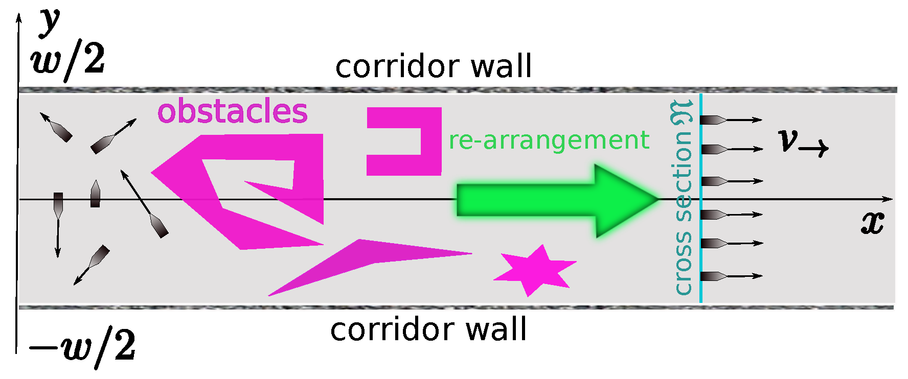
3. Sweep Coverage of a Corridor
Formal Problem Statement
- (i)
- Any USV i does not collide with the obstacles , the walls of the corridor , and the other USVs ;
- (ii)
- There is and an enumeration of the USVs such that .
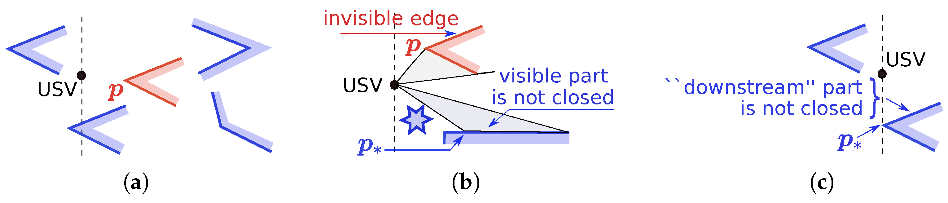
4. Theoretical Assumptions About the Scenario
- (i)
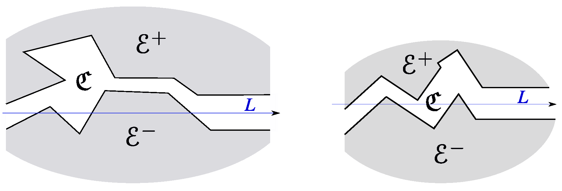
- It is open and goes from the boundary of the obstacle ;
- (ii)
- This ray is not -free;
- (iii)
- To the left of and arbitrarily close to it, there is an upward/downward ray that is -free.
5. Navigation Algorithm: Preprocessing Sensory Data
- and ;
- No obstacle separates USVs j and ;
- If some of them (say j) lie below/above a visor, then the ordinate of the other USV is less/greater than that of this visor provided that USV is to the left of USV j.
- (B.1)
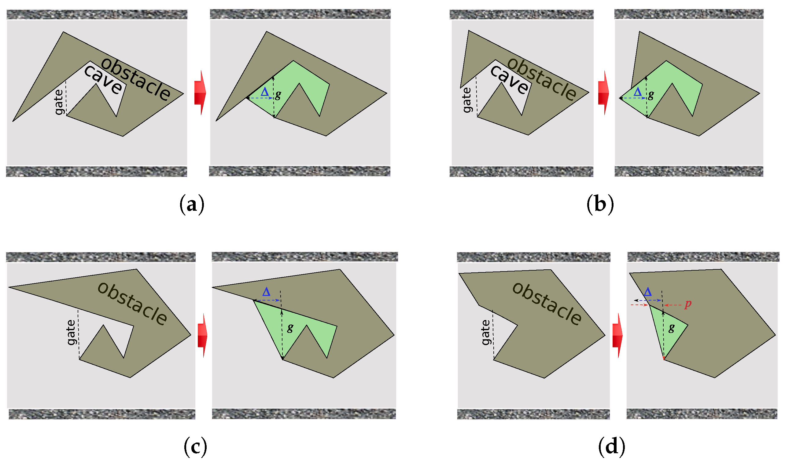
- Vertically below/above USV i “identifies” an obstacle at a distance ;
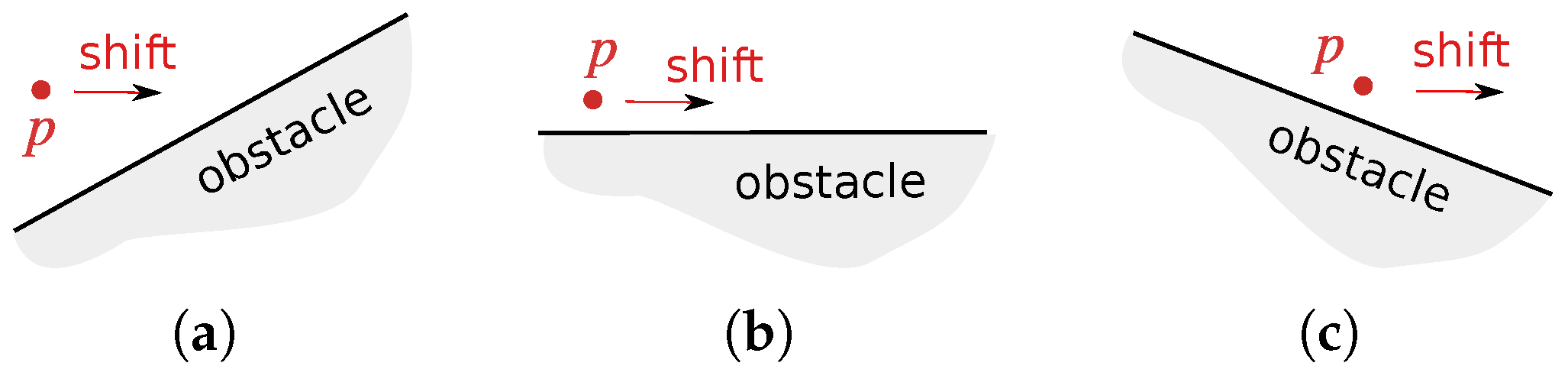
- (B.2)
- If , then the infinitesimal shift of in the x direction does not increase the vertical distance from to the obstacles (see Figure 6);
- (B.3)
- If for a link in , then the infinitesimal plane-parallel shift of in the x direction does not increase the vertical distance from to the obstacles.
6. Navigation Algorithm
7. Main Results
7.1. Preliminaries
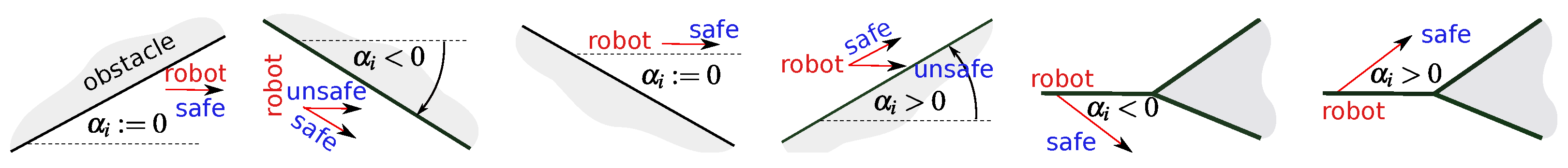
- , length of the x-scope of the compact set E, i.e., ;
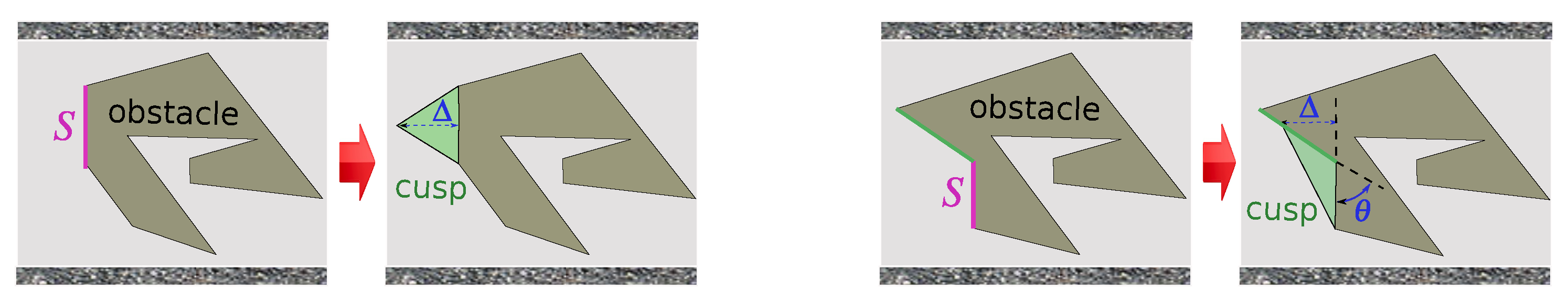
- , polar angle of a non-vertical segment S oriented in the ascending direction of x;
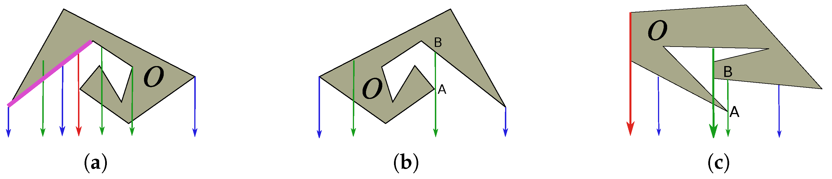
- , collection of all globally upper/lower sides of all ’s (see Definition 3 and Figure 3).
7.2. Key Theoretical Result
- (i)
- The control generated by the proposed navigation law always satisfies the inequality from (1), as is required;
- (ii)
- The USVs sweep the scene with a speed of , as defined in Definition 1;
- (iii)
- Their x scatter does not grow as time progresses;
- (iv)
- Any USV moves along the corridor in the targeted direction: for almost all t;
- (v)
- The USVs travel at distinct distances from the corridor walls: ;
- (vi)
- The ordering of the USVs in the vertical direction does not change with time.
7.3. Discussion of the Key Theoretical Result
7.4. Secondary Add-Ons to Theorem 1
7.5. Dropout of Team Members
7.6. Addition to the Team
7.7. Non-Straight Corridors
- (i)
- The sets are simply connected and form a partition of ;
- (ii)
- There are and such that, in a right-handed Cartesian frame whose abscissa axis is L, the parts of the sets , and lying to the right of the abscissa are described by the inequalities , and , respectively, along with ;
- (iii)
- Assumption 2 is true for and .
7.8. Some Hints to Relax Assumption 2
8. Computer Simulation Tests
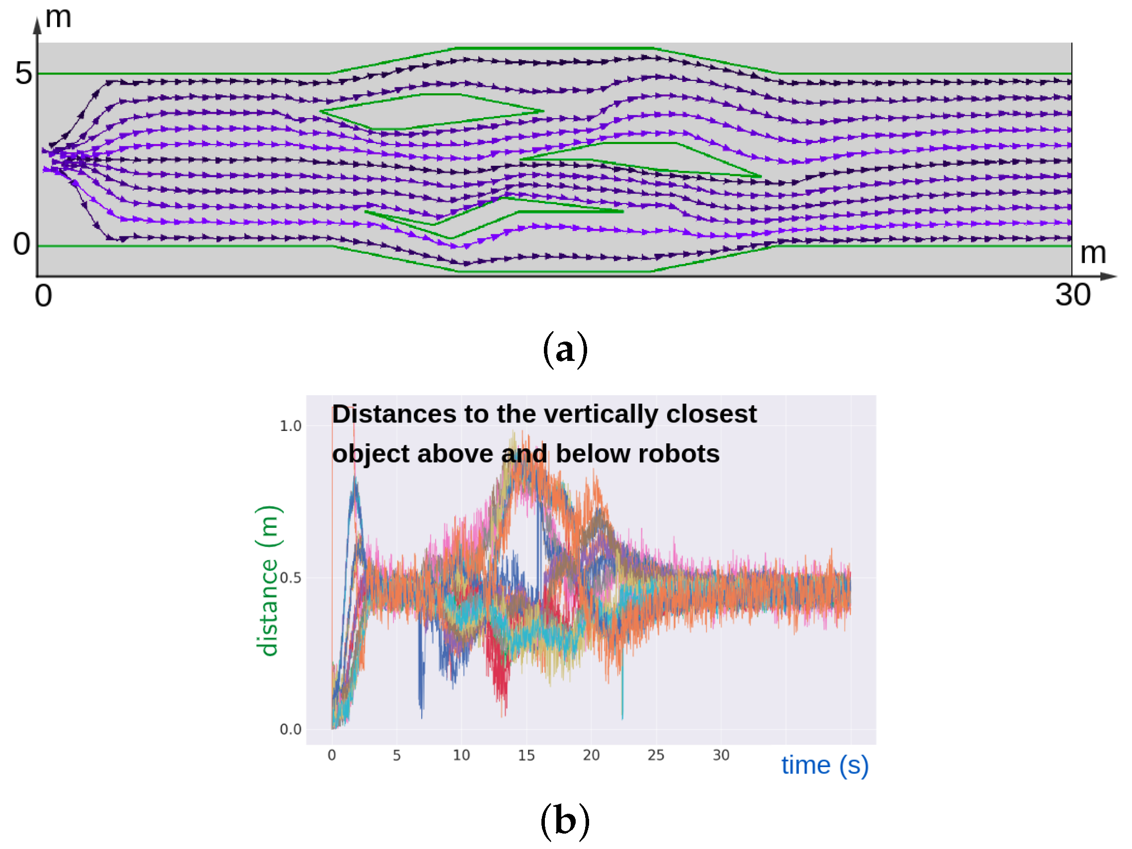
8.1. Numerical Experiments
8.2. Gazebo Experiments
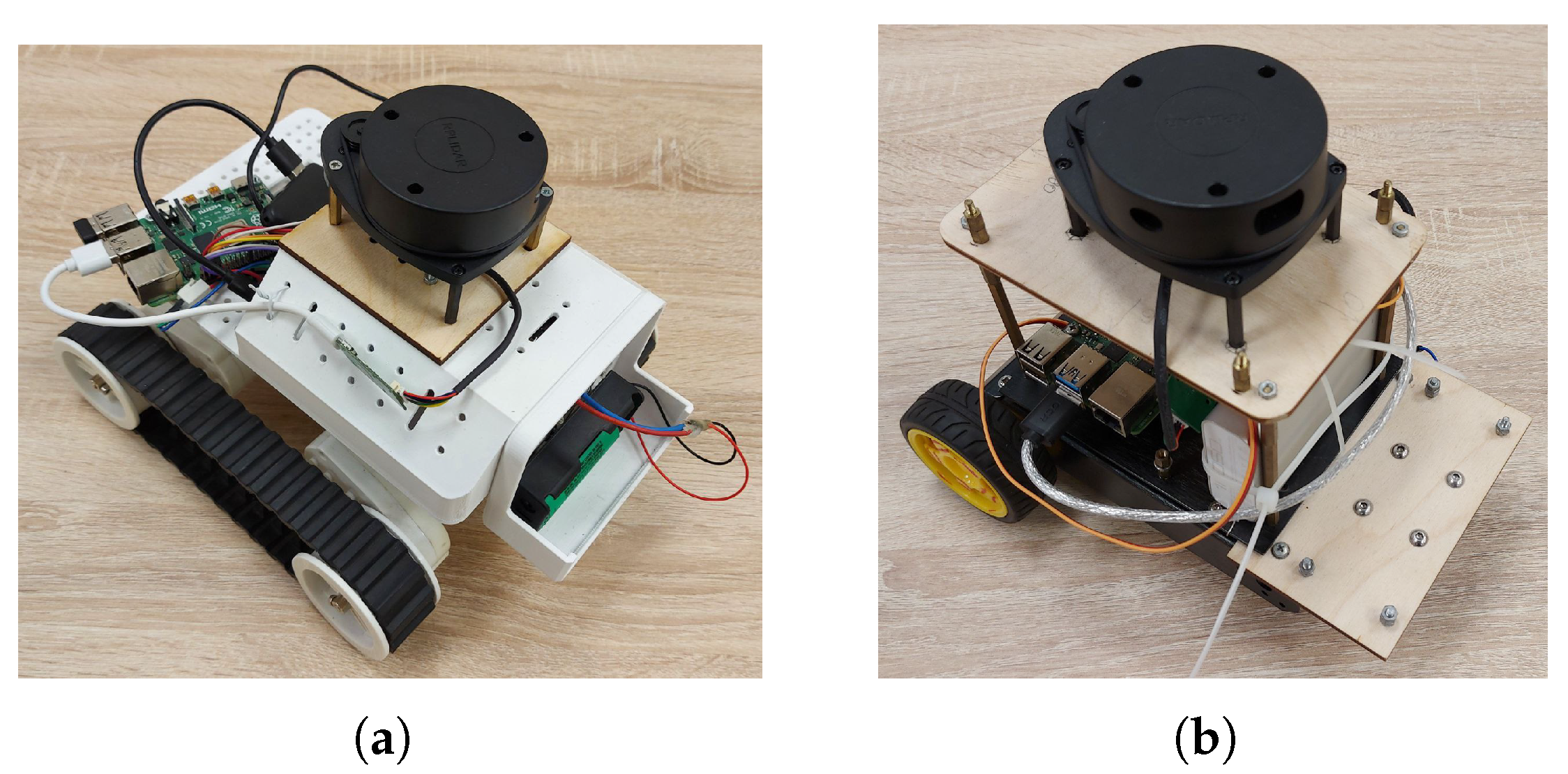
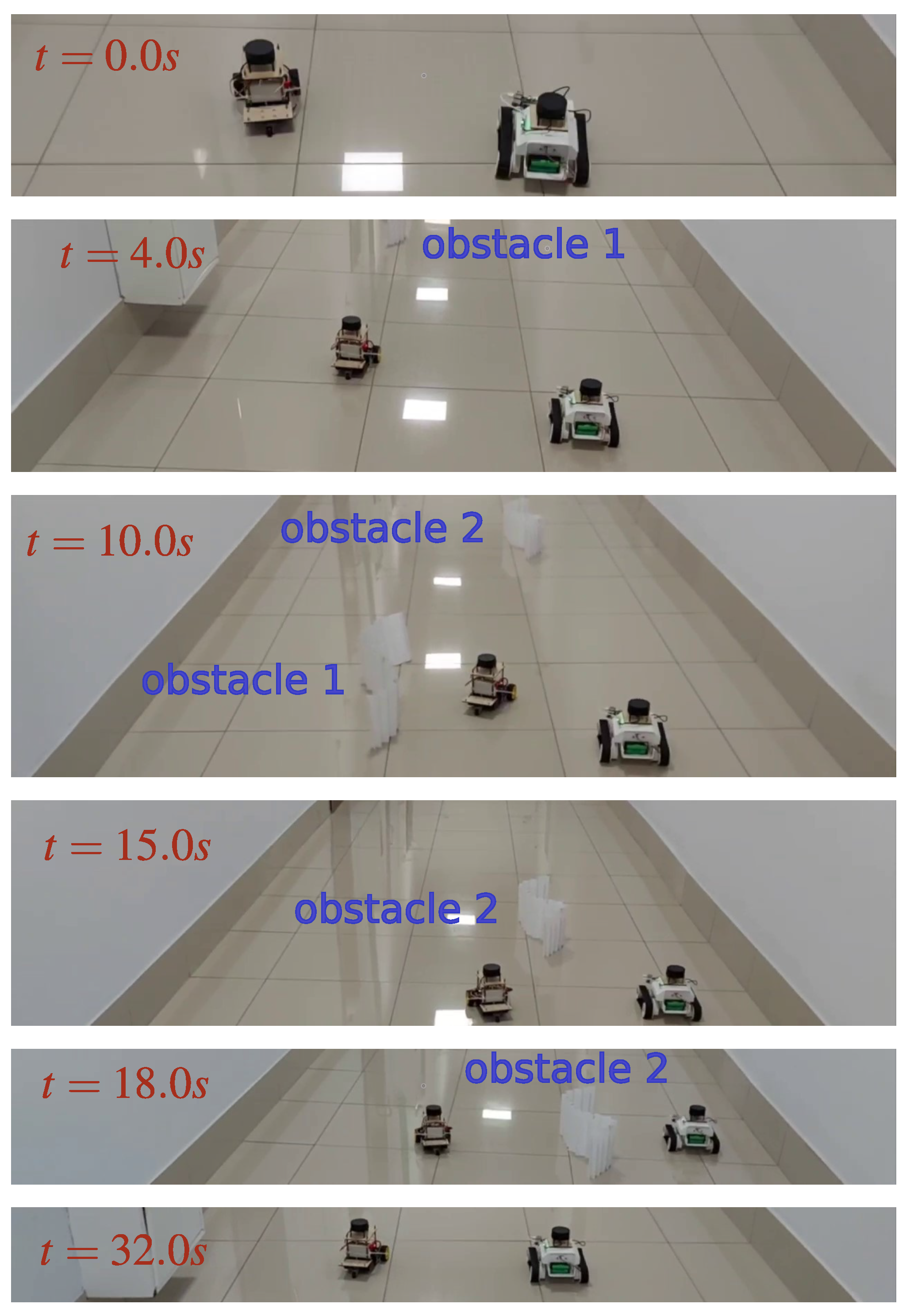
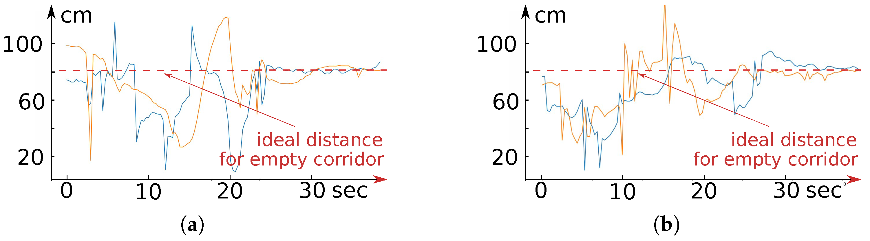
9. Results of Real-World Tests
10. Conclusions and Future Work
Supplementary Materials
Author Contributions
Funding
Data Availability Statement
Conflicts of Interest
Abbreviations
| USV | Unmanned surface vehicle |
| a.a. | “for almost all” |
| Conventions and notations | |
| Positive angles | counted counterclockwise |
| “is defined to be”, “is used to denote” | |
| “segment of a line” | its part between two points |
| “segment” | “segment of a straight line” |
| segment bridging the points | |
| minus | |
| minus | |
| minus and | |
| number of elements in the set A | |
| signum function, | |
| boundary of the set O | |
| coordinates of point | |
| ∅ | empty set |
| handled corridor | |
| w | width of the corridor |
| N | number of the robots |
| kth obstacle | |
| location of robot i | |
| coordinates of robot i | |
| velocity vector of robot i | |
| upper bound on the robot’s speeds | |
| desired speed | |
| sensing distance | |
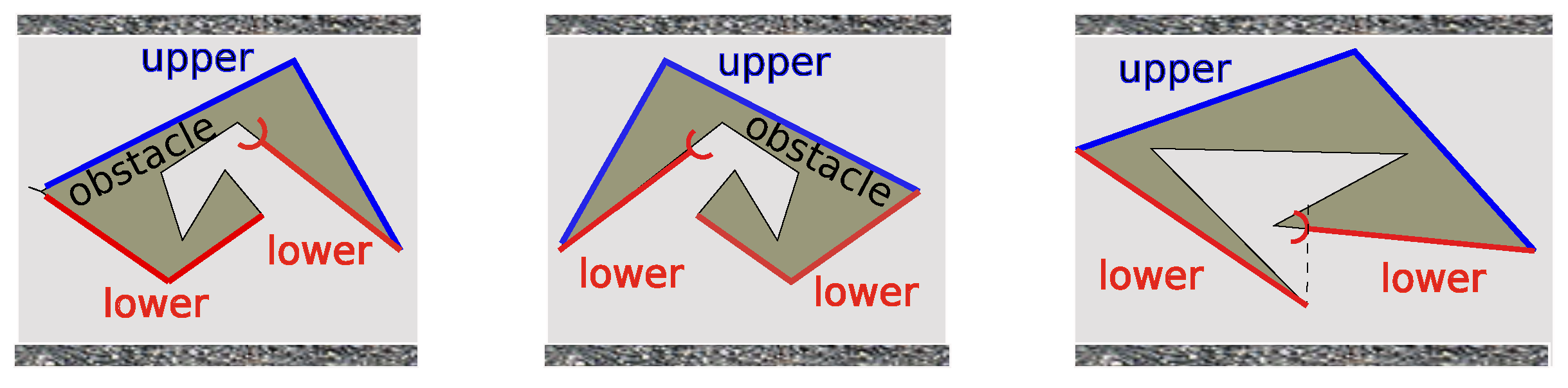
| upper/lower fences of obstacle | |
| upper bound on the polar angles of the segments in upper and lower fences | |
| controller parameters | |
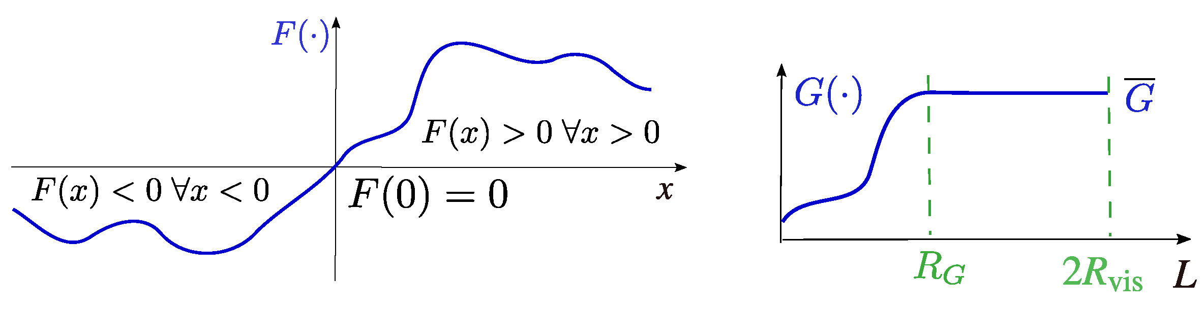
| functions used to build the controller | |
Appendix A. Proof of Theorem 1 and Remarks 2, 3, and 4
- (i)
- For , USV i is not in the caves of any obstacle ;
- (ii)
- If there is a point of an obstacle that lies above (below) , the closest of such points belongs to the lower (upper) fence of .
- (i)
- No more than one obstacle affects the bases and of USV i.
- (ii)
- No more than one base is not empty.
- (i)
- Either one and only one of the locations lies in the x scope of the obstacle , or the both lie there and are vertically aligned ;
- (ii)
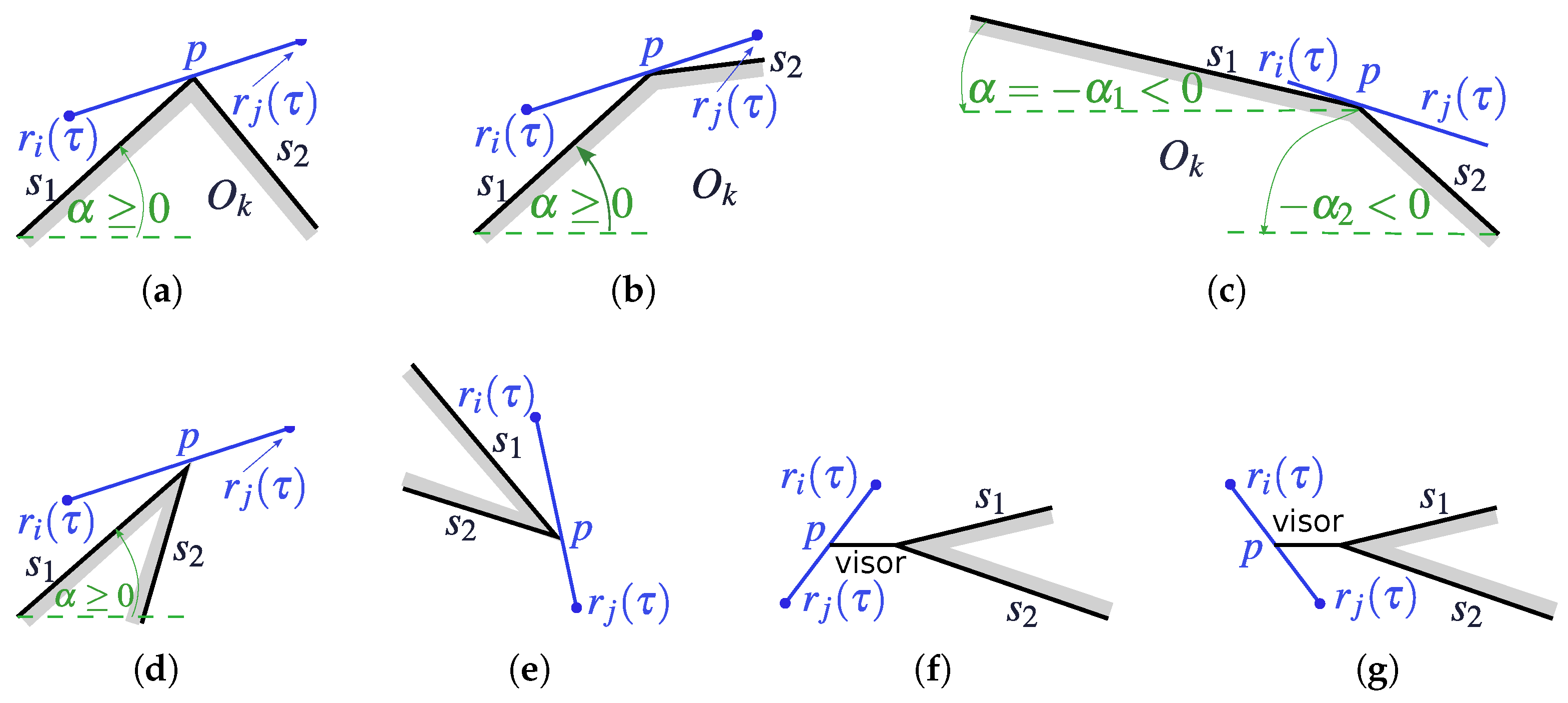
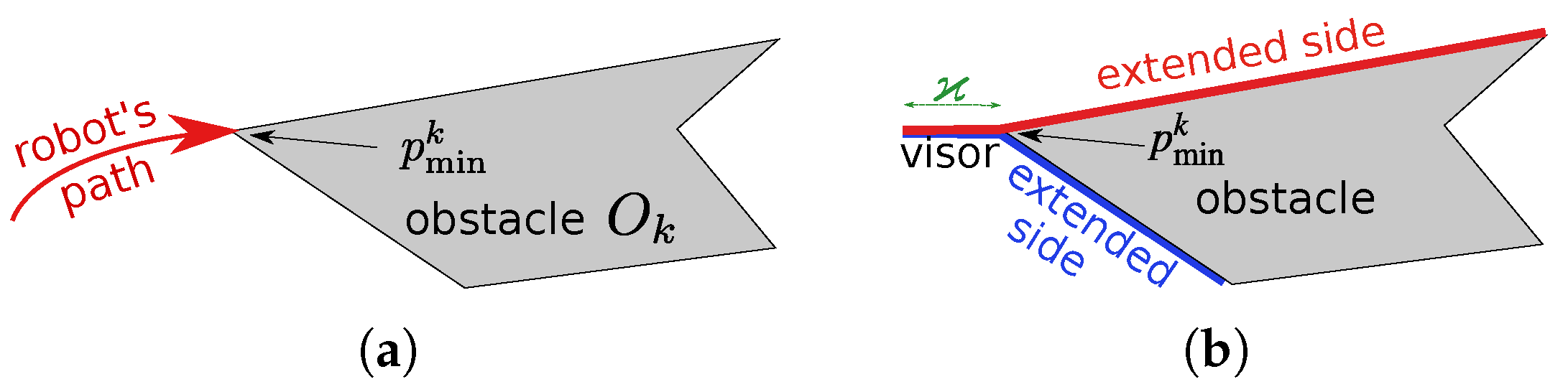
- Any is either the left end of a visor or a right cape (see Figure A3e–g);
- (b.1)
- , where ;
- (b.2)
- for .
References
- Xing, T.; Liu, Y.; Chen, L. Survey of robot formation control methods. Acad. J. Sci. Technol. 2022, 4, 58–61. [Google Scholar] [CrossRef]
- Oh, K.; Park, M.; Ahn, H. A survey of multi-agent formation control. Automatica 2015, 53, 424–440. [Google Scholar] [CrossRef]
- Werger, B. Cooperation without deliberation: A minimal behavior-based approach to multi-robot teams. Artif. Intell. 1999, 110, 293–320. [Google Scholar] [CrossRef]
- Abdelli, A.; Amamra, A.; Yachir, A. Swarm Robotics: A Survey. In Advances in Computing Systems and Applications; Senouci, M., Boulahia, S., Benatia, M., Eds.; Springer: Cham, Switzerland, 2022; pp. 153–164. [Google Scholar]
- Xu, D.; Zhang, X.; Zhu, Z.; Chen, C.; Yang, P. Behavior-Based Formation Control of Swarm Robots. Math. Probl. Eng. 2014, 2014, 205759. [Google Scholar] [CrossRef]
- Ren, W.; Beard, R. Distributed Consensus in Multi-Vehicle Cooperative Control: Theory and Applications; Springer: London, UK, 2008. [Google Scholar]
- Li, Y.; Tan, C. A survey of the consensus for multi-agent systems. Syst. Sci. Control. Eng. 2019, 7, 468–482. [Google Scholar] [CrossRef]
- Maghenem, M.; Loria, A.; Nuno, E.; Panteley, E. Consensus-based formation control of networked nonholonomic vehicles with delayed communications. IEEE Trans. Autom. Control. 2021, 66, 2242–2249. [Google Scholar] [CrossRef]
- Savkin, A.; Cheng, T.; Xi, Z.; Javed, F.; Matveev, A.; Nguyen, H. Decentralized Coverage Control Problems for Mobile Robotic Sensor and Actuator Networks; Wiley and IEEE Press: Hoboken, NJ, USA, 2015. [Google Scholar]
- Wu, W.; Zhang, Z.; Lee, W.; Du, D. Sweep-Coverage. In Optimal Coverage in Wireless Sensor Networks; Springer Optimization and Its Applications; Springer: Berlin/Heidelberg, Germany, 2020; Volume 261, pp. 183–192. [Google Scholar]
- Huang, H.; Savkin, A.; Ding, M.; Huang, C. Mobile robots in wireless sensor networks: A survey on tasks. Comput. Netw. 2019, 148, 1–19. [Google Scholar] [CrossRef]
- Gage, D. Command control for many-robot systems. In Proceedings of the the 19th Annual AUVS Technical Symposium, Hunstville, AL, USA, 22–24 June 1992; Volume 4, pp. 22–24. [Google Scholar]
- Ding, L.; Han, Q.; Ge, X.; Zhang, X. An overview of recent advances in event-triggered consensus of multiagent systems. IEEE Trans. Cybern. 2018, 48, 1110–1123. [Google Scholar] [CrossRef]
- Wen, G.; Yu, X.; Yu, W.; Lu, J. Coordination and control of complex network systems with switching topologies: A Survey. IEEE Trans. Syst. Man Cybern. Syst. 2021, 51, 6342–6357. [Google Scholar] [CrossRef]
- Ji, M.; Egerstedt, M. Distributed coordination control of multiagent systems while preserving connectedness. IEEE Trans. Robot. 2007, 23, 693–703. [Google Scholar] [CrossRef]
- Dimarogonas, D.; Kyriakopoulos, K. Connectedness preserving distributed swarm aggregation for multiple kinematic robots. IEEE Trans. Robot. 2008, 24, 1213–1223. [Google Scholar] [CrossRef]
- Yang, Y.; Shi, Y.; Constantinescu, D. Connectivity-preserving synchronization of time delay Euler–Lagrange networks with bounded actuation. IEEE Trans. Cybern. 2019, 51, 3469–3482. [Google Scholar] [CrossRef] [PubMed]
- Zavlanos, M.; Pappas, G. Distributed connectivity control of mobile networks. IEEE Trans. Robot. 2008, 24, 1416–1428. [Google Scholar] [CrossRef]
- Kan, Z.; Navaravong, L.; Shea, J.; Pasiliao, E.; Dixon, W. Graph matching-based formation reconfiguration of networked agents with connectivity maintenance. IEEE Trans. Control. Netw. Syst. 2015, 2, 24–35. [Google Scholar] [CrossRef]
- Poonawala, H.; Spong, M. Preserving strong connectivity in directed proximity graphs. IEEE Trans. Autom. Control. 2017, 62, 4392–4404. [Google Scholar] [CrossRef]
- Lin, H.; Huang, Y. Collaborative complete coverage and path planning for multi-robot exploration. Sensors 2021, 11, 3709. [Google Scholar] [CrossRef]
- Ni, J.; Gu, Y.; Tang, G.; Ke, C.; Gu, Y. Cooperative coverage path planning for multi-mobile robots based on improved K-means clustering and deep reinforcement learning. Electronics 2024, 13, 944. [Google Scholar] [CrossRef]
- Muhsen, D.; Sadiq, A.; Raheem, F. A survey on swarm robotics for area coverage problem. Algorithms 2024, 17, 3. [Google Scholar] [CrossRef]
- Heo, N.; Varshney, P. Energy-efficient deployment of intelligent mobile sensor networks. IEEE Trans. Syst. Man Cybern. Part A 2005, 35, 78–92. [Google Scholar] [CrossRef]
- Chao, H.; Chen, Y.; Ren, W. A study of grouping effect on mobile actuator sensor networks for distributed feedback control of diffusion process using central Voronoi tessellations. Int. J. Robot. Res. 2006, 11, 185–190. [Google Scholar]
- Wang, Y.; Tseng, Y. Distributed deployment schemes for mobile wireless sensor networks to ensure multilevel coverage. IEEE Trans. Parallel Distrributed Syst. 2008, 19, 1280–1294. [Google Scholar] [CrossRef]
- Deif, D.; Gadallah, Y. Classification of wireless sensor networks deployment techniques. IEEE Commun. Surv. Tutor. 2014, 16, 834–855. [Google Scholar] [CrossRef]
- Chang, C.; Chin, Y.; Chen, C.; Chang, C. Impasse-aware node placement mechanism for wireless sensor networks. IEEE Trans. Syst. Man Cybern. Syst. 2018, 48, 1225–1237. [Google Scholar] [CrossRef]
- Zhou, M.; Li, J.; Wang, C.; Wang, J.; Wang, L. Applications of Voronoi diagrams in multi-robot coverage: A Review. J. Mar. Sci. Eng. 2024, 12, 1022. [Google Scholar] [CrossRef]
- Sadeghi, M.; Shahrabi, A.; Ghoreyshi, S.; Alfouzan, F. Distributed node deployment algorithms in mobile wireless sensor networks: Survey and challenges. ACM Trans. Sens. Netw. 2023, 19, 91. [Google Scholar]
- Houssein, E.; Saad, M.; Djenouri, Y.; Hu, G.; Ali, A.; Shabah, H. Metaheuristic algorithms and their applications in wireless sensor networks: Review, open issues, and challenges. Clust. Comput. 2024, 27, 13643–13673. [Google Scholar] [CrossRef]
- Wei, C.; Ji, Z.; Cai, B. Particle swarm optimization for cooperative multi-robot task allocation: A multi-objective approach. IEEE Robot. Autom. Lett. 2020, 5, 2530–2537. [Google Scholar] [CrossRef]
- Rossides, G.; Metcalfe, B.; Hunter, A. Particle swarm optimization—An adaptation for the control of robotic swarms. Robotics 2021, 10, 58. [Google Scholar] [CrossRef]
- Spears, W.; Spears, D.; Heil, R.; Kerr, W.; Hettiarachchi, S. An overview of physicomimetics. In Proceedings of the International Workshop on Swarm Robotics, Santa Monica, CA, USA, 17 July 2004; Şahin, E., Spears, W.M., Eds.; Springer: Berlin/Heidelberg, Germany, 2005; pp. 84–97. [Google Scholar]
- Schwager, M.; Rus, D.; Slotine, J. Decentralized, adaptive coverage control for networked robots. Int. J. Robot. Res. 2009, 28, 357–375. [Google Scholar] [CrossRef]
- Razafindralambo, T.; Simplot-Ryl, D. Connectivity preservation and coverage schemes for wireless sensor networks. IEEE Trans. Autom. Control. 2011, 56, 6819–6820. [Google Scholar] [CrossRef]
- Rout, M.; Roy, R. Self-deployment of randomly scattered mobile sensors to achieve barrier coverage. IEEE Sens. J. 2016, 16, 6819–6820. [Google Scholar] [CrossRef]
- Chowdhury, T.J.; Elkin, C.; Devabhaktuni, V.; Rawat, D.B.; Oluoch, J. Advances on localization techniques for wireless sensor networks: A survey. Comput. Netw. 2016, 110, 284–305. [Google Scholar] [CrossRef]
- Bartolini, N.; Ciavarella, S.; Silvestri, S.; Porta, T.L. On the vulnerabilities of Voronoi-based approaches to mobile sensor deployment. IEEE Trans. Mob. Comput. 2016, 15, 3114–3128. [Google Scholar] [CrossRef]
- Mahboubi, H.; Aghdam, A. Distributed deployment algorithms for coverage improvement in a network of wireless mobile sensors: Relocation by virtual force. IEEE Trans. Control. Netw. Syst. 2017, 4, 736–748. [Google Scholar] [CrossRef]
- Zhou, D.; Wang, Z.; Bandyopadhyay, S.; Schwager, M. Fast, on-line collision avoidance for dynamic vehicles using buffered Voronoi cells. IEEE Robot. Autom. Lett. 2017, 2, 1047–1054. [Google Scholar] [CrossRef]
- Elmokadem, T.; Savkin, A. Computationally-efficient distributed algorithms of navigation of teams of autonomous UAVs for 3D coverage and flocking. Drones 2021, 5, 124. [Google Scholar] [CrossRef]
- Eledlebi, K.; Ruta, D.; Hildmann, H.; Saffre, F.; Al Hammadi, Y.; Isakovic, A.F. Coverage and energy analysis of mobile sensor nodes in obstructed noisy indoor environment: A Voronoi-approach. IEEE Trans. Mob. Comput. 2022, 21, 2745–2760. [Google Scholar] [CrossRef]
- Bartolini, N.; Calamoneri, T.; Ciavarella, S.; La Porta, T.; Silvestri, S. Autonomous mobile sensor placement in complex environments. ACM Trans. Auton. Adapt. Syst. 2017, 12, 7. [Google Scholar] [CrossRef]
- Priyadarshi, R.; Gupta, B.; Anurag, A. Deployment techniques in wireless sensor networks: A survey, classification, challenges, and future research issues. J. Supercomput. 2022, 76, 7333–7373. [Google Scholar] [CrossRef]
- Zhou, Z.; Chen, T.; Wu, D.; Yu, C. Corridor navigation and obstacle distance estimation for monocular vision mobile robots. Int. J. Digit. Content Technol. Its Appl. 2011, 5, 192–202. [Google Scholar]
- Keshavan, J.; Gremillion, G.; Alvarez-Escobar, H.; Humbert, J. Autonomous vision-based navigation of a quadrotor in corridor-like environments. Int. J. Micro Air Veh. 2015, 7, 111–123. [Google Scholar] [CrossRef]
- Gupta, S.; Sangeeta, R.; Mishra, R.; Singal, G.; Badal, T.; Garg, D. Corridor segmentation for automatic robot navigation in indoor environment using edge devices. Comput. Netw. 2020, 178, 107374. [Google Scholar] [CrossRef]
- Pang, Y.; Zhou, L.; Lin, B.; Lv, G.; Zhang, C. Generation of navigation networks for corridor spaces based on indoor visibility map. Int. J. Geogr. Inf. Sci. 2020, 34, 177–201. [Google Scholar] [CrossRef]
- Padhy, R.; Ahmad, S.; Verma, S.; Bakshi, S.; Sa, P. Localization of unmanned aerial vehicles in corridor environments using deep learning. In Proceedings of the the 25th International Conference on Pattern Recognition (ICPR), Milan, Italy, 10–15 January 2021; pp. 9423–9428. [Google Scholar]
- Aneesh, P.; Singh, R.; Dash, R. Autonomous UAV navigation in indoor corridor environments by a depth estimator based on a deep neural network. In Proceedings of the the 15th International Conference on Computing Communication and Networking Technologies (ICCCNT), Kamand, India, 24–28 June 2024; pp. 1–5. [Google Scholar]
- Cheng, T.; Savkin, A. Decentralized control for mobile robotic sensor network self-deployment: Barrier and sweep coverage problems. Robotica 2011, 29, 283–294. [Google Scholar] [CrossRef]
- Chen, C.; Liu, S.; Zhong, C.; Zhang, B. Multiple robot formation control strategy in corridor environments. In Proceedings of the the 33rd Chinese Control Conference, Nanjing, China, 28–30 July 2014; pp. 8507–8512. [Google Scholar]
- Shi, M.; Qin, K.; Liu, J. Cooperative multi-agent sweep coverage control for unknown areas of irregular shape. IET Control. Theory Appl. 2018, 12, 1983–1994. [Google Scholar] [CrossRef]
- Matveev, A.; Konovalov, P. Distributed reactive motion control for dense cooperative sweep coverage of corridor environments by swarms of non-holonomic robots. Int. J. Control. 2023, 96, 554–567. [Google Scholar] [CrossRef]
- Matveev, A.; Konovalov, P.; Gordievich, K.; Gusev, S. Distributed reactive navigation of robotic teams for sweep coverage of a corridor environment with an obstacle course. In Proceedings of the the 7th International Conference on Robotics and Automation Engineering (ICRAE), Singapore, 18–20 November 2022; pp. 210–214. [Google Scholar]
- Filippov, A. Differential Equations with Discontinuous Righthand Sides; Kluwer Academic Publishers: Dordrecht, The Netherlands, 1988. [Google Scholar]
- Lin, Z.; Francis, B.; Maggiore, M. State agreement for continuous-time coupled nonlinear systems. SIAM J. Control. Optim. 2007, 46, 288–307. [Google Scholar] [CrossRef]
- Zavlanos, M.; Egerstedt, M.; Pappas, G. Graph-theoretic connectivity control of mobile robot networks. Proc. IEEE 2011, 99, 1525–1540. [Google Scholar] [CrossRef]
- Kan, Z.; Dani, A.; Shea, J.; Dixon, W. Network connectivity preserving formation stabilization and obstacle avoidance via a decentralized controller. IEEE Trans. Autom. Control. 2012, 57, 1827–1832. [Google Scholar] [CrossRef]
- Matveev, A.; Wang, C.; Savkin, A. Real-time navigation of mobile robots in problems of border patrolling and avoiding collisions with moving and deforming obstacles. Robot. Auton. Syst. 2012, 60, 769–788. [Google Scholar] [CrossRef]
- Matveev, A.; Hoy, M.; Katupitiyac, J.; Savkin, A. Nonlinear sliding mode control of an unmanned agricultural tractor in the presence of sliding and control saturation. Robot. Auton. Syst. 2013, 61, 973–987. [Google Scholar] [CrossRef]
- Danskin, J. The theory of min-max, with applications. SIAM J. Appl. Math. 1966, 14, 641–644. [Google Scholar] [CrossRef]
- Hartman, P. Ordinary Differential Equations, 2nd ed.; Birkhäuzer: Boston, MA, USA, 1982. [Google Scholar]
- Matveev, A.; Novinitsyn, I.; Proskurnikov, A. Stability of continuous-time consensus algorithms for switching networks with bidirectional interaction. In Proceedings of the 2013 European Control Conference, Zurich, Switzerland, 17–19 July 2013; pp. 1872–1877. [Google Scholar]

| = 6.0 m/s | = 1.5 m | = 1.0 m/s |
| P = 2.0 m/s | ||
| 1/s | ||
| = 20 ms |
| = 1.5 m/s | = 4.0 m | = 0.3 m/s |
| P = 2.0 m/s | /4 rad | |
| 1/s | ||
| = 200 ms |
Disclaimer/Publisher’s Note: The statements, opinions and data contained in all publications are solely those of the individual author(s) and contributor(s) and not of MDPI and/or the editor(s). MDPI and/or the editor(s) disclaim responsibility for any injury to people or property resulting from any ideas, methods, instructions or products referred to in the content. |
© 2025 by the authors. Licensee MDPI, Basel, Switzerland. This article is an open access article distributed under the terms and conditions of the Creative Commons Attribution (CC BY) license (https://creativecommons.org/licenses/by/4.0/).
Share and Cite
Konovalov, P.; Matveev, A.; Gordievich, K. Reactive Autonomous Ad Hoc Self-Organization of Homogeneous Teams of Unmanned Surface Vehicles for Sweep Coverage of a Passageway with an Obstacle Course. Drones 2025, 9, 161. https://doi.org/10.3390/drones9030161
Konovalov P, Matveev A, Gordievich K. Reactive Autonomous Ad Hoc Self-Organization of Homogeneous Teams of Unmanned Surface Vehicles for Sweep Coverage of a Passageway with an Obstacle Course. Drones. 2025; 9(3):161. https://doi.org/10.3390/drones9030161
Chicago/Turabian StyleKonovalov, Petr, Alexey Matveev, and Kirill Gordievich. 2025. "Reactive Autonomous Ad Hoc Self-Organization of Homogeneous Teams of Unmanned Surface Vehicles for Sweep Coverage of a Passageway with an Obstacle Course" Drones 9, no. 3: 161. https://doi.org/10.3390/drones9030161
APA StyleKonovalov, P., Matveev, A., & Gordievich, K. (2025). Reactive Autonomous Ad Hoc Self-Organization of Homogeneous Teams of Unmanned Surface Vehicles for Sweep Coverage of a Passageway with an Obstacle Course. Drones, 9(3), 161. https://doi.org/10.3390/drones9030161