Article

A Method for UAV Path Planning Based on G-MAPONet Reinforcement Learning

1
College of Civil Aviation, Nanjing University of Aeronautics and Astronautics, Nanjing 211106, China
2
College of General Aviation and Flight, Nanjing University of Aeronautics and Astronautics, Nanjing 211106, China
*
Author to whom correspondence should be addressed.
Drones 2025, 9(12), 871; https://doi.org/10.3390/drones9120871
Submission received: 25 October 2025 / Revised: 8 December 2025 / Accepted: 15 December 2025 / Published: 17 December 2025

Highlights

What are the main findings?
  • A hierarchical attention and collaborative framework combining GAT and MHA layers is proposed, which captures dynamic spatiotemporal features and realizes multi-scale path planning, overcoming the limitations of static models and resolving global–local conflicts.
  • The GRPO algorithm is applied to optimize UAV path planning strategies, improving convergence speed and policy stability; experiments show that G-MAPONet outperforms traditional and single-attention models in diverse scenarios in terms of convergence, reward, and task completion.
What are the implications of the main findings?
  • The proposed framework provides an effective solution for dynamic environmental modeling and multi-scale optimization in UAV path planning, enhancing adaptability to complex environments.
  • The integration of hierarchical mechanisms and GRPO offers theoretical and technical references for intelligent trajectory planning in other multi-agent systems or dynamic task scenarios.

Abstract

To address the issues of efficiency and robustness in UAV trajectory planning under complex environments, this paper proposes a Graph Multi-Head Attention Policy Optimization Network (G-MAPONet) algorithm that integrates Graph Attention (GAT), Multi-Head Attention (MHA), and Group Relative Policy Optimization (GRPO). The algorithm adopts a three-layer architecture of “GAT layer for local feature perception–MHA for global semantic reasoning–GRPO for policy optimization”, comprehensively achieving the goals of dynamic graph convolution quantization and global adaptive parallel decoupled dynamic strategy adjustment. Comparative experiments in multi-dimensional spatial environments demonstrate that the Gat_Mha combined mechanism exhibits significant superiority compared to single attention mechanisms, which verifies the efficient representation capability of the dual-layer hybrid attention mechanism in capturing environmental features. Additionally, ablation experiments integrating Gat, Mha, and GRPO algorithms confirm that the dual-layer fusion mechanism of Gat and Mha yields better improvement effects. Finally, comparisons with traditional reinforcement learning algorithms across multiple performance metrics show that the G-MAPONet algorithm reduces the number of convergence episodes (NCE) by an average of more than 19.14%, increases the average reward (AR) by over 16.20%, and successfully completes all dynamic path planning (PPTC) tasks; meanwhile, the algorithm’s reward values and obstacle avoidance success rate are significantly higher than those of other algorithms. Compared with the baseline APF algorithm, its reward value is improved by 8.66%, and the obstacle avoidance repetition rate is also enhanced, which further verifies the effectiveness of the improved G-MAPONet algorithm. In summary, through the dual-layer complementary mode of GAT and MHA, the G-MAPONet algorithm overcomes the bottlenecks of traditional dynamic environment modeling and multi-scale optimization, enhances the decision-making capability of UAVs in unstructured environments, and provides a new technical solution for trajectory planning in intelligent logistics and distribution.

1. Introduction

The research on the optimal path planning of UAVs plays an important role in enhancing the efficiency and intelligence of logistics distribution. In recent years, relevant studies have made significant progress mainly in the directions of complex environment adaptation, refined management of uncertainty, and multi-task sharing and collaboration. For dynamic environments, an enhanced velocity field method integrated with PD control effectively enables UAV obstacle avoidance [1], offering a novel approach for motion control. Comparatively, two-stage stochastic programming combined with scene decomposition algorithms demonstrates superior efficacy in uncertain environments for material distribution [2]. Similarly, multi-stage programming models focus on end-to-end decision-making in humanitarian logistics [3], integrating resource deployment and facility allocation to support complex emergency scenarios. In urban multi-objective distribution, the Binary Hybrid Particle Swarm Optimization (BHPSO) algorithm [4] reduces computational burdens and enables efficient dynamic task scheduling. However, its suboptimal trajectory smoothness incurs additional costs—a limitation addressed by dynamic coverage point estimation with B-spline path planning [5]. Further precision requirements for multi-layer spatial distribution are met through distance/time-minimized path optimization models [6]. Collectively, in-depth research on UAV trajectory planning scenarios has effectively improved the planning efficiency of UAVs, reduced their operating costs, expanded the market space of the low-altitude economy, and simultaneously promoted the development of intelligent low-altitude operation technologies.
Early drone path planning research predominantly employed heuristic algorithms. These methods, however, struggle significantly with dynamic environment adaptation and effective multi-drone collaboration. While bi-level programming improves macroscopic network topology and traffic distribution optimization [7], its predefined structure lacks real-time obstacle adaptability. Similarly, Matching Optimization and Mixed Integer Linear Programming (MILP) enhance task allocation [8,9] but overlook dynamic UAV constraints and communication network time-dependency. Meta-heuristic algorithms excel in 3D path planning. The Multi-objective Crow Search Optimization (MOCSO_TA) and Dung Beetle Optimization (DBO) leverage swarm behaviors to balance objectives and altitude variations. Yet, their computational complexity surges in obstacle-dense environments [10,11]. Glowworm Swarm Optimization (GSO) suffers from local convergence in dynamic settings, necessitating specialized objective functions [12,13]. Dijkstra-based geometric methods enable short-distance load balancing [14] but perform poorly in complex terrain. Crucially, traditional heuristics assume static conditions. They cannot model dynamic elements like obstacle trajectories [15,16], depend excessively on prior information, and exhibit weak collaboration in heterogeneous UAV swarms—hindering load balancing and strategy consistency. Their global optimization capability is also inadequate in high-dimensional spaces; genetic algorithms [17] and particle swarm optimization [18] frequently converge to local optima in complex scenarios. Reliance on fixed topologies or pre-trained models further limits adaptability, neglecting data-driven modeling [19] and real-world environmental integration [20]. Compared to Capacitated Vehicle Routing Problem (CVRP) or PSO, traditional methods respond inefficiently to dynamic traffic in critical applications like medical emergencies [21]. The core limitation across these approaches remains the inability to dynamically model “UAVs–environment–tasks” interactions, degrading path planning efficiency—especially in challenging terrains or multi-agent scenarios.
This paper proposes G-MAPONet, a UAV path planning framework for logistics applications that enhances the GRPO algorithm through the integration of GAT and MHA layers to overcome key performance bottlenecks. The main contributions are as follows:
(1)
Hierarchical attention modeling of dynamic spatiotemporal features: A dual-layer fusion mechanism combining GAT and MHA layers is designed. The dynamic graph model captures time-varying environmental weights, and multi-head computation identifies UAV traversal patterns. Experiments show that this dual-layer mechanism improves convergence efficiency and overcomes the limits of static models.
(2)
Hierarchical collaborative mechanism for multi-scale path planning: The framework uses high-level MHA for global guidance and low-level GAT for local optimization. The high-level module generates a trajectory based on terrain trends, while the low-level module enables real-time obstacle avoidance. This design resolves the global–local conflict in single-scale planning.
(3)
Objective and constraint modeling: A composite objective function integrates timeliness compliance and energy efficiency. A multi-constraint model includes flight altitude, payload, speed, and delivery time.
(4)
Efficient strategy optimization under GRPO: The GRPO algorithm is applied to UAV path planning. By adjusting the trust region to regulate step size, it improves convergence speed and policy stability.
(5)
Robustness and generalization across scenarios: Experiments in diverse environments show that G-MAPONet outperforms traditional and single-attention models in convergence, reward, and task completion.
The paper is organized as follows: Section 2 introduces the GAT and MHA mechanisms and proposes the G-MAPONet architecture. Section 3 describes the objective and constraint models, simulation environments, and comparative experiments. Section 4 evaluates the performance of different methods. Section 5 summarizes the work and outlines future directions.

2. Materials and Methods

2.1. Related Research Content

Data-driven reinforcement learning (RL) methods offer a new approach to dynamic path planning. However, challenges remain in sample efficiency, multi-machine collaboration, and feature modeling. Distributed RL improves multi-UAV coverage using the “centralized training-decentralized execution” framework, but policy collapse occurs under limited communication due to poor environmental understanding [22]. The dynamic uncertainty quantization mechanism eases data convergence issues in discrete RL, but fails to model physical interactions between UAVs [10]. Multi-UAV RL clusters struggle with “credit assignment.” For example, the Centralized-S Proximal Policy Optimization (C-SPPO) framework uses attention mechanisms for task allocation but still faces conflicts during topology changes [23]. Hybrid clustering and Multi-Agent Reinforcement Learning (MARL) frameworks depend on fixed communication structures, limiting adaptability to dynamic task shifts [24]. Single RL algorithms rely on manual reward design, making it hard to meet multiple goals like shorter paths, lower energy use, and better obstacle avoidance [25]. Inverse RL (IRL) is limited by the generalization of historical data [26]. High-dimensional spaces pose a “curse of dimensionality”; transfer learning needs large datasets to converge [27]. Hybrid methods like the improved bat algorithm [28] and RL-gray wolf optimization [29] combine heuristics with RL but still depend on manual rewards and lack point-to-point learning. RL also shows delays in dynamic settings. Sequential convex optimization improves efficiency [30] but is slow to detect sudden obstacles. Improved multidimensional optimization [31] and Rapidly Exploring Random Tree Star (RRT*) algorithms [32] speed up convergence but lack dynamic modeling in attention-based systems. Multi-UAV strategies also lack consistency. The State-Action-Reward-State-Action (SARSA) based routing algorithm ignores UAV energy differences [33], and average reward-punishment mechanisms overlook UAV diversity [34]. Model Predictive [35]. Control-Reinforcement Learning (MPC-RL) frameworks allow real-time obstacle avoidance but miss temporal-spatial dynamics [36]. Multi-UAV control strategies handle topology changes but ignore dynamic obstacles [37,38]. Finally, Deep Q-Network (DQN) based methods improve generalization but rely heavily on prediction models, limiting real-time adaptability [39].
The attention mechanism improves information processing through dynamic weighting, but UAV path planning still faces challenges like coarse interaction modeling and delayed response. The Ant Colony Optimization–Deep Q-Network–Time Parameter (ACO-DQN-TP) framework uses adaptive steps and attention-based networks to adjust trajectory smoothness, but lacks obstacle speed prediction [40]. The Partially Observable Weighted Mean Field Reinforcement Learning (PO-WMFDDPG) algorithm handles large-scale UAV actions but ignores UAV heterogeneity [34]. Graph neural networks learn node weights automatically, but their attention updates cannot keep up with environmental changes [41]. Multi-scale fusion algorithms struggle to combine global planning with local replanning. For example, combining potential fields with MARL enables obstacle avoidance, but without attention, threat levels are poorly differentiated [42]. The 3D visibility graph improves efficiency but relies on static structures, limiting real-time updates [43]. A multi-objective algorithm models UAV energy use but does not update weights dynamically with attention [44]. Attention and policy gradients are only loosely integrated. The Graph Attention Networks–Reinforcement Learning (GAT-RL) controller models vehicle interaction but not 3D UAV swarms [45]. Though the rabbit optimization algorithm with heat search has been proposed, an attention-based multi-UAV cooperation strategy is missing [46].
Based on the comprehensive analysis above, to achieve dynamic environment adaptation and deep integration with policy gradients, this paper proposes a G-MAPONet algorithm. Through the synergistic effect of the GAT layer (Graph Attention Network, optimizing fine-grained interactive modeling of nodes) and the MHA layer (Multi-Head Attention, dynamically adjusting attention weight allocation), targeted optimization and upgrading of the GRPO algorithm are conducted.

2.2. G-MAPONet Fusion Algorithm Design

2.2.1. G-MAPONet Model Framework

G-MAPONet is a three-layer algorithm that integrates the attention mechanisms of the GAT (Graph Attention Network) layer and MHA (Multi-Head Attention) layer. Its core design idea is to combine the GAT and MHA mechanisms to achieve a full-process closed loop of “environment perception-feature interaction-action decision-making”, and the overall logic is illustrated in Figure 1. Next, the design concepts of each module are explained as follows: The 3D spatial grid environment module is utilized to construct the basic environment covering the start point, target point, and trajectory, providing core scene information support for the entire algorithm framework; The GAT layer realizes local interaction of node features by normalizing attention weights via the Softmax function; The MHA layer generates Q, K, and V vectors through scaled dot-product attention to complete feature concatenation; The GRPO layer incorporates target distance and obstacle parameters, and ultimately outputs UAV control actions.
Positioned in the upper-left quadrant of Figure 1 is the definition of the 3D aerial spatial grid environment, which delineates the start point, target endpoint, and optimal trajectory path of the dynamic trajectory. The lower-left quadrant corresponds to the GAT layer: subsequent to the computation of attention weights, multiple node features are aggregated via Softmax normalization, thereby enabling local feature interaction. The lower-right quadrant denotes the MHA layer: via scaled dot-product attention, coupled with linear transformations, this layer facilitates the generation of Q, K, and V vectors alongside feature concatenation. Features processed by this dual-attention mechanism are fed into the GRPO layer, which conducts network feature computation by incorporating target distance (Lg) and obstacle (Ob) parameters. The derived action outputs are subsequently transmitted to the UAV attitude control component situated in the upper-right quadrant. This entire framework encompasses the full workflow from environmental perception to the output of UAV action decisions. It ensures precise attitude updating and output, while delivering a dynamic programming solution tailored to UAVs operating within complex environments.

2.2.2. Model Pseudocode

The G-MAPONet fusion algorithm is detailed in Algorithm 1, encompassing Actor network initialization, experience buffer configuration, and the parameter settings for GAT and MHA. During each training iteration, the environment is reset, local spatial features are extracted via the GAT module, and global semantic representations are derived through MHA inference. Following state updates, the policy samples actions for environment interaction and stores the resulting experiences. Subsequently, the generalized advantage estimation (GAE) is calculated and normalized, serving as the basis for batch-wise Actor policy updates guided by loss functions and KL divergence. The final optimized policy model is then output, facilitating efficient modeling and decision-making in complex environments.
Algorithm 1: G-MAPONet
   Input: Initialize parameters l , δ , γ , Q ,   K ,   V , ε ,   θ , i , j , X b
    W Q , W K , W V
   Number of Steps T; State Space Dimension d s ; Action Space Dimension d a ;
   Number of GAT Heads M g a t ; Hidden Layer Dimension d h ; Episode E
   Output: The Optimized G-MAPONet Model π θ
1  π θ = ActorNetwork ( d s , d a )
2  D = ReplayBuffer ( )
3  W gat m = RandomMatrix ( d h , d s ) ;   α gat m = RandomMatrix ( 2 d h )
4  W mha Q = RandomMatrix ( d h , d h ) ;   W mha K = RandomMatrix ( d h , d h ) ; W mha V = RandomMatrix ( d h , d h ) ;   W mha O = RandomMatrix ( d h , d h )
5  for   epoch   =   1   to   E   do
6         for   t   =   0   to   T   1   do
7                 for   m   =   1   to   M gat do
8                         H m = W gat m H 0
9                         for each ( i , j ) do
10                                  e i , j , m = LeakyReLU ( α gat m ) T [ H m [ i ] ; H m [ j ] ]
11                         end
12                         h i , m = j ( i ) W i , j , m H m [ j ]
13                         Z gat = Concat ELU ( h i , 1 ) , ELU ( h i , 2 ) , ELU ( h i , M gat )
14                 end
15                 Q = X b W Q ;   K = X b W Q ;   V = X b W Q
16                 attention = Softmax ( scores ) ;   context = attention V ;   s t = context W O
17                 a t = π θ ( s t ) + σ ( 0 , I ) ;   ( s t + 1 , r t , done ) = envstep ( a t )
18                 if done then
19                         break
20                 end
21         end
22         for t   =   T   1   to   0 do
23                 δ t = r t + ε V [ t + 1 ] ( 1 done t ) V [ t ] ;   A [ t ] = δ t + ε l A [ t + 1 ] ( 1 done t )
24         end
25         A = ( A mean ( A ) ) / ( std ( A ) + C )
26         for b a t c h D do
27                 r ( θ ) = π θ ( s batch , a batch ) / ( π θ ( s batch ) ) ;   J ( θ ) = E [ r ( θ ) A batch ]
28                 θ = θ + γ ( J ) / J T J + C
29                 if   K L ( π old , π new ) > δ then
30                         θ = θ η ( θ θ old )
31                 end
32         end
33         y batch = r batch + ε V φ ( s t + 1 ) ( 1 done batch )
34         L V = 1 B i = 1 B ( V φ ( s batch [ i ] ) y batch [ i ] ) 2
35         φ = φ γ L V
36  end
37  return   π θ

2.2.3. Algorithm Inference Process

The GAT layer model, as described in Section 2.3, is formulated as follows:
H k = W gat k H 0 h i , k = j ( i ) e x p LeakyReLU ( α gat k ) T [ H k [ i ] ; H k [ j ] ] m ( i ) e x p ( e i , m , k ) H k [ j ] Z gat = Concat ELU ( h i , 1 ) , ELU ( h i , 1 ) , , ELU ( h i , K gat )
The MHA layer, as detailed in Section 2.4, performs dimension splicing on multiple feature vectors. Input features are projected into distinct subspaces via linear transformations, allowing the model to capture diverse attention patterns. The association strength between elements in the input sequence is then computed using scaled dot-product attention:
δ = Q = X b W Q K = X b W K V = X b W V s t = Softmax Q K T d model / h V W O
Table A1 lists the meanings of s t and other parameters in Equation (2). The UAV, working with the policy network, interacts with the environment and updates its actions iteratively through balanced exploration in the state space:
a t = π θ ( s t ) + σ ( 0 , I )
Table A1 defines the representative meanings of σ and ( 0 , I ) in Equation (3). σ ( 0 , I ) denotes exploration noise that improves the policy’s exploration capability, and π θ ( s t ) represents the policy network:
( s t + 1 , r t , done ) = envstep ( a t )
In Formula (4), s t + 1 represents that at time t, performing action a t leads to the environment transitioning to the next state, r t represents the after performing action a t at time t, the immediate reward obtained by the drone from the environment, and done represents the Boolean value indicating whether the cyclic task has ended. envstep ( a t ) represents the environment update triggered by executing a t , which calculates the value estimation deviation based on the difference between the actual reward received and the estimated value V [ t ] in the current:
δ t = r t + ε V [ t + 1 ] ( 1 done t ) V [ t ]
In Formula (5), ε represents the discount factor, V [ t ] represents the measuring the advantage of taking a certain action at time t relative to the average policy, done t represents the termination flag, and δ t represents the value network at time t state   s t value estimate. A [ t + 1 ] denotes the value estimation of the next state s t at time t + 1. The combination of the temporal difference error δ t and the advantage A [ t + 1 ] from the next time step reduces advantage estimation variance and enhances training stability:
A [ t ] = δ t + ε l A [ t + 1 ] ( 1 done t )
In Formula (6), A [ t ] represents the advantage of taking a certain action at time t relative to the average policy, l represents the generalized advantage estimation parameter, with a range of values between (0,1), used to dynamically balance the bias and variance fluctuation range, and λ represents the regularization coefficient. When λ equals 0, the generalized advantage estimation relies solely on the temporal difference error δ t ; when λ equals 1, the method approximates the Monte Carlo approach. Standardizing the advantage function A to have zero mean and unit variance effectively enhances training stability by mitigating the impact of extreme potential values:
A = A mean ( A ) std ( A ) + C
In Formula (7), mean ( A ) represents the mean of A, std ( A ) represents the standard deviation of A, and C represents the constant. The importance sampling ratio quantifies the likelihood ratio of the updated policy and the old policy selecting the same action under identical state conditions. This enables ongoing policy updates based on data generated by the older policy. The importance sampling ratio is defined as:
r ( θ ) = π θ ( s batch , a batch ) π θ ( s batch )
In Formula (8), a batch represents the action actually executed in state s batch , s batch represents the state representation in a batch of data, A batch represents the advantage values corresponding to batch data, π θ represents the updated policy, r ( θ ) represents the importance sampling ratio, and θ represents the parameters of the policy function   π θ . π θ ( s batch , a batch ) denotes the probability of selecting action a batch in state s batch under the updated strategy π θ , while π θ ( s batch ) represents the total probability of taking any action in state s batch under the same strategy. By weighting advantage A batch with the importance sampling ratio r ( θ ) , the model enhances the selection probability of actions with higher advantages, thereby effectively maximizing expected returns. The expected return objective function for strategy θ is:
J ( θ ) = E [ r ( θ ) A batch ]
In Formula (9), E [ ] represents the expectation, J represents the gradient vector, and J ( θ ) represents the objective function of the policy’s expected return. The application of the chain rule to compute the partial derivatives of each parameter in J ( θ ) determines the direction of parameter updates and finalizes the backpropagation algorithm. The gradient vector J is obtained as follows:
J = J ( θ ) θ
The strategy is optimized to maximize expected returns, and the parameters of the strategy network are updated through gradient ascent as follows θ :
θ = θ + γ J J T J + C
In the Formula (11), γ represents the learning rate, and δ the preset trust region value. J J T J + C denotes gradient normalization, a mechanism that prevents the generation of large gradient moduli and thereby avoids unstable training. Should the new strategy perform significantly worse than the previous one—specifically, if KL divergence exceeds threshold δ —a rollback is implemented to prevent strategy collapse caused by excessive update amplitude.
KL ( π old , π new ) > δ θ = θ η ( θ θ old )
In the Formula (12), π old represents the old policy, π new represents the new policy, and η represents the step size backoff coefficient. KL ( π old , π new ) denotes the KL divergence between the old strategy π old and the new strategy π new , quantifying the extent of their difference. During the current batch data training, actual rewards are used to guide the training of the value network. That is, the value network is:
y batch = r batch + ε V φ ( s t + 1 ) ( 1 done batch )
In the Formula (13), r batch represents the immediate reward of the batch data, ε represents the discount factor, V φ ( s t + 1 ) represents the value estimation of the next state by the value network, s t + 1 represents the next state, done batch represents the termination flag of the batch data, and L V represents the loss function of the value network. The prediction error of the value network is quantified by computing the average squared difference between the estimated and target values. The parameters of the network are optimized through minimization of the loss function. Consequently, the mean squared error of loss function L V is derived [47]:
L V = 1 B i = 1 B ( V φ ( s batch [ i ] ) y batch [ i ] ) 2
In Formula (14), V φ represents the value network, φ represents the parameters of the value network, and B represents the batch size. V φ ( s batch [ i ] ) denotes the value network’s estimation of s batch [ i ] based on batch data, while y batch [ i ] represents the associated target value. The value network is updated through the following procedure:
φ = φ γ L V
In Formula (15), γ represents the learning rate, and L V represents gradient of the Loss Function L V with Respect to Value Network Parameters φ .

2.3. GAT Layer Attention Mechanism

The GAT layer (Graph Attention Network) is a graph-based neural network that learns node association weights adaptively through an attention mechanism, without requiring predefined graph structures. As shown in Algorithm 2, the process includes linear transformation of node features, calculation of unnormalized node pair scores using LeakyReLU-activated attention parameters, Softmax normalization for neighbor weights, aggregation of neighbor information, and enhancement of feature representation via multi-head attention concatenation. Its key advantages are adaptive weight learning, local structure perception, flexibility, and parallel computing capability.
Algorithm 2: GAT
   Input: Initialize parameters i , j , d f , d h , m   , M   , Γ   , Γ b , γ , λ ; Episode E,
   Grid environment G
   Output: Optimized GAT model parameter Θ
1  W m = RandomMatrix ( d h , d f )
2  α m = RandomVector ( 2 d h )
3  for epoch   =   1   to   Episode   do
4         for each G   do
5                 H 0 = ExtractNodeFeatures ( G )
6                 for m   =   1   to M do
7                         H m = W gat m H 0
8                         for each   ( i , j )     G   do
9                                   e i , j , m = LeakyReLU ( α gat m ) T [ H m [ i ] ; H m [ j ] ]
10                         end
11                         W i , j , m = exp ( e i , j , m ) / w ( i ) exp ( e i , w , m )
12                         h i , m = j ( i ) W i , j , m H m [ j ]
13                 end
14                 Z gat = Concat ELU ( h i , 1 ) , ELU ( h i , 2 ) , ELU ( h i , M g a t )
15                 Γ b = ComputeLoss ( ξ , T )
16                 Γ = Γ + Γ b + λ | | Θ | | 2 2
17                 Θ = Θ γ Θ Γ
18         end
19  end
20  return Θ
Initialize the attention head weights of the input features mapped to the hidden layer W m and a vector of attention score parameters for inter-node α m , For each attention from 1 to M the corresponding weight matrix with attention parameter vector is:
W m = RandomMatrix ( d h , d f )   m { 1 , 2 , , M } α m = RandomVector ( 2 d h )       m { 1 , 2 , , M }
In Formula (16), d h represents the dimension of the hidden layer, d f represents the dimension of input features, and M represents the number of attention heads. For each GAT attention head m , the feature matrix H 0 undergoes a linear transformation using the weight matrix W gat m . The resulting feature matrix after the m-th attention head transformation in GAT is:
H m = W gat m H 0
In Formula (17), H 0 represents the initial feature matrix input to GAT, W gat m represents Weight matrix of the m-th attention head in the GAT model. The attention score between node i and node j is computed by first taking the dot product of the joint representation of node features and the attention parameter vector, then scaling it by ( α gat m ) T , concatenating the result into vector [ H m [ i ] ; H m [ j ] ] , and finally applying the LeakyReLU activation function:
e i , j , m = LeakyReLU ( α gat m ) T [ H m [ i ] ; H m [ j ] ]
In Formula (18), α gat m represents the attention parameter vector of the m-th GAT attention head; H m [ i ] represents In the m-th attention head of GAT, the feature vector of node i after feature transformation; and H m [ j ] represents In the m-th attention head of GAT, the feature vector of node j after feature transformation. [ H m [ i ] ; H m [ j ] ] denotes the concatenation of the feature-transformed vectors from nodes i and j, forming a combined vector. LeakyReLU refers to an activation function that introduces nonlinearity to mitigate the problem of gradient vanishing. Given input x, the formula can be expressed as:
LeakyReLU ( x ) = x x 0 C x x < 0
In Formula (19), C represents Constant, and e i , w , m represents The unnormalized attention score between node i and domain node ω . During subsequent feature aggregation, the attention weights are normalized using the following approach:
W i , j , m = e x p ( e i , j , m ) w ( i ) e x p ( e i , w , m )
In Formula (20), W i , j , m represents the normalized attention weight of node i for neighbor node j under the m-th attention head, e i , j , m represents Attention score between node i and node j under the m-th attention head. ( i ) represents the set of neighboring nodes associated with node i. The normalized attention weight e i , j , m is applied to weight and sum the features H m [ j ] of node i neighbors, enabling effective aggregation of neighborhood information and yielding more representative node features:
h i , m = j ( i ) W i , j , m H m [ j ]
The Formula (21), j ( i ) denotes the sum of all nodes j in the set of node i domain. The multi-head mechanism enables the model to learn different spatial feature representations and complete multi-information synthesis through splicing as a way to complete the model’s ability to represent and capture complex patterns. Next, each GAT output feature h i , m is introduced as a nonlinear feature after applying the ELU activation function, and then the M gat GAT header features are output spliced along the feature dimension, and the final output GAT feature Z gat is:
Z gat = Concat ELU ( h i , 1 ) , ELU ( h i , 2 ) , , ELU ( h i , M gat )
In Formula (22), M gat represents the number of attention heads in GAT. Concat denotes the concatenation operation, which combines multiple feature vectors into a unified representation. ELU represents the exponential linear unit (ELU), an activation function specifically designed to introduce nonlinearity into the model:
ELU ( x ) = x x 0 C ( e x 1 ) x < 0
In Formula (23), C represents Constant and x represents the input value of nonlinear feature. Following the concatenation of multi-head attention outputs, the model applies both the loss function and regularization to optimize learning:
Γ b = ComputeLoss ( ξ , T ) Γ = Γ + Γ b + λ | | Θ | | 2 2
In Formula (24), Γ b represents Loss values of the current batch data, ξ represents the input of the current batch of data, T represents the target value, λ represents the regularization coefficient, and Θ represents the set of all parameters learned by the model. | | Θ | | 2 2 represents L2 regularization. The total loss Γ is minimized by squaring the Θ norm to refine the model parameters:
Θ = Θ γ Θ Γ
In the Formula (25), γ represents the learning rate. Θ Γ represents the gradient of the loss function Γ with respect to parameter Θ , capturing the direction and magnitude of the parameter’s influence on the loss function.

2.4. MHA Layer Attention Mechanism

The MHA layer (Multi-Head Attention mechanism) serves as the core component of the Transformer model. It enhances model expressiveness by computing multiple attention heads in parallel across distinct subspaces. As illustrated in Algorithm 3, the process comprises: generating Q, K, and V from input features using learned weight matrices; calculating attention scores through scaled dot product and normalizing these scores with Softmax; deriving the context vector by weighting and summing V; and concatenating the outputs from all heads, followed by a linear transformation to recover the original dimension. This mechanism supports the capture of multi-dimensional relationships, modeling of global dependencies, and efficient computation.
Algorithm 3: MHA
   Input: Initialize parameters i , h , d model , X b , W Q , W K , W V
    Z h , a , Γ
   Output: Attention-Enhanced Sequence Z
1  W Q = RandomMatrix ( d model , d model / h )
2  W K = RandomMatrix ( d model , d model / h )
3  W V = RandomMatrix ( d model , d model / h )
4  W O = RandomMatrix ( h d model / h , d model )
5  for   epoch   =   1   to   Episode   do
6           for each   X b   do
7                     Q = X b W Q ;   K = X b W K ;   V = X b W V
8                     scores = Q K T / d model / h
9                     attention = Softmax ( scores )
10                   context = attention V
11                   for i   =   1   to h do
12                         Q i = Q : , : , i d model h : ( i + 1 ) d model h
13                         K i = K : , : , i d model h : ( i + 1 ) d model h
14                         V i = V : , : , i d model h : ( i + 1 ) d model h
15                         Z h = Concat ( context 1 , context 2 , , context h )
16                   end
17                   Z = Z h W O
18                   Γ = ComputeLoss ( Z , T )
19                   W Q = W Q γ W Q Γ
20                   W K = W K γ W K Γ
21                   W V = W V γ W V Γ
22                   W O = W O γ W O Γ
23           end
24  end
25  return   Ζ
Initialize the query, key, value, and output weight matrices, denoted as W Q , W K , W V , and W O , respectively, which are the learnable parameters of the model:
W Q = RandomMatrix ( d model , d model / h ) W K = RandomMatrix ( d model , d model / h ) W V = RandomMatrix ( d model , d model / h ) W O = RandomMatrix ( h d model / h , d model )
In Formula (26), W Q represents the query weight matrix, W K represents key weight matrix, W V represents the value weight matrix, W O represents output weight matrix, d model represents the feature dimension of the model, and h represents the number of heads in the multi-head attention mechanism. The query matrix Q, key matrix K, and value matrix V are derived through linear transformations of the weight matrices as follows:
Q = X b W Q K = X b W K V = X b W V
In Equation (27), X b represents the input feature matrix for each batch. The correlation strength between elements of the input sequence is computed by scaling the dot product of the query and key matrices to derive the attention score matrix scores, which is subsequently normalized to obtain matrix attention. The value matrix V is then aggregated through a weighted sum using the attention weights to produce the output vector context.
scores = Q K T d model / h attention = Softmax ( scores ) context = attention V
In Equation (28), Q K T represents the calculate the dot product of the query matrix and the key matrix. Here, d model / h denotes the scaling factor, Softmax represents the normalization of raw attention scores into a probability distribution, attention indicates the resulting attention weight matrix, and context corresponds to the application of these weights to the value matrix V, Q, K, and V are split into h submatrices based on the number of attention heads, and all head outputs Z h are concatenated as described:
Q i = Q : , : , i d m o d e l h : ( i + 1 ) d m o d e l h K i = K : , : , i d m o d e l h : ( i + 1 ) d m o d e l h V i = V : , : , i d m o d e l h : ( i + 1 ) d m o d e l h Z h = Concat ( context 1 , context 2 , , context h )
In Formula (29), Q represents the query matrix, K represents the key matrix, and V represents the value matrix. Q i denotes the query sub-matrix of the i-th attention head, K i the key sub-matrix, V i the value sub-matrix, and context i the vector generated by the i-th attention head. The attention-enhanced sequence is derived by applying a linear transformation to the concatenated multi-head outputs via the output weight matrix:
Z = Z h W O
In Formula (30), Z h represents the matrix after multi-head attention concatenation. The gradient is derived through backpropagation to compute the output cross-entropy loss:
Γ = ComputeLoss ( Z , T ) W Q = W Q γ W Q Γ W K = W K γ W K Γ W V = W V γ W V Γ W O = W O γ W O Γ
In the Formula (31), γ represents the learning rate, Z represents the model final output feature matrix, and T represents the target value. W Q Γ , W K Γ , W V Γ , and W O Γ represent the gradients of the loss function Γ with respect to the weight matrices W Q , W K , W V , and W O , respectively.

3. Experiment and Results

3.1. Distribution Route Planning and Design

3.1.1. Objective Function Design

The logistics unmanned aerial vehicle distribution center is set as p 0 , and the set of distribution path nodes is p = { p 1 , p 2 , , p n } . Among them, g { p i , p j } represents the distance between the distribution points p i and p j . The path set of the first unmanned aerial vehicle L i = { p i 1 , p i 2 , , p i n i } , and the objective function for constructing the Maximum timeliness compliance rate (MTCR) and Minimum energy consumption (MEC) function F of the logistics UAV distribution is shown in Formula (32):
F = k = 1 n i 1 g ( p i , k , p i , k + 1 ) v i + g ( p i , n i , p 0 ) v i MTCR + i = 1 n ρ k = 1 n i 1 ϑ i , k g ( p i , k , p i , k + 1 ) + ϑ i , n i g ( p i , n i , p 0 ) MEC
In Formula (32), v i represents the UAV flight speed, ϑ i , k represents the load of the i-th UAV at the k-th node, ϑ i , n i represents the load at the delivery node n i of the i-th UAV, and ρ represents the energy consumption coefficient per unit load distance. g ( p i , k , p i , k + 1 ) denotes the flight distance of the i-th drone from p i , k to p i , k + 1 , and g ( p i , n i , p 0 ) represents the distance from the last node of the i-th drone to p 0 . ϑ i , n i g ( p i , n i , p 0 ) indicates the energy consumption of the i-th drone during its return to the node. When a return trip is present, the product of the return distance g ( p i , n i , p 0 ) and the end load ϑ i , n i must be considered to accurately reflect the load’s effect on return energy consumption. In the absence of a return trip, setting ϑ i , n i to 0 or p to 1 ensures that re turn energy consumption is 0.

3.1.2. Flight Environment Constraints

Flight Altitude Constraint
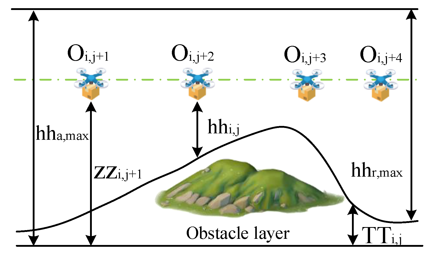
The flight altitude of logistics drones is subject to the constraints depicted in Figure 2 [48]. Specifically, TT i , j denotes the altitude of the i-th route at the j-th track point; zz i , j represents the corresponding sea-level reference altitude; hh r , max indicates the relative flight altitude; and hh a , max defines the maximum allowable absolute flight altitude.
Develop a model for the height restrictions of logistics UAV:
HH i , j = ς ( hh a , max TT i , j )   if   ( z z i , j TT i , j ) > hh a , max z z i , j                           else   TT i , j < ( z z i , j TT i , j ) < hh a , max ς ( hh i j + TT i , j )         else   ( z z i , j TT i , j ) < 0
In the Formula (33), O i , j + 1 , O i , j + 2 , O i , j + 3 and O i , j + 4 denote the j + 1 , j + 2 , j + 3 and j + 4 waypoints along the i-th route, respectively. ς represents the height coefficient, with a value range of (0, 1). HH i , j denotes the actual flight altitude at the j-th waypoint of the i-th route.
UAV Payload Constraint
The payload constraint in UAV path planning needs to satisfy:
v i FF max 2 G 2 ff d
In the Formula (34), v i represents the horizontal flight speed, G represents the total takeoff weight, ff d represents the drag coefficient, and FF max represents the maximum limit of the total flight pull force.
Speed Constraint
The flight speed v i of the UAV during path planning must meet the following restrictions:
v min v i v max
In the Formula (35), the minimum flight speed V min 5   m s 1 and the maximum flight speed V max 14   m s 1 are determined based on the safety flight speed limit, ensuring that the drone’s flight speed remains within the safe and compliant range at all times.
Time Constraint
The time t i required for the logistics drone to perform path planning must satisfy:
t i T max
Due to limitations such as energy consumption and machine performance, the maximum time of T max 20 min must satisfy the constraints.

3.2. Experimental Scenarios

3.2.1. Experimental Procedure

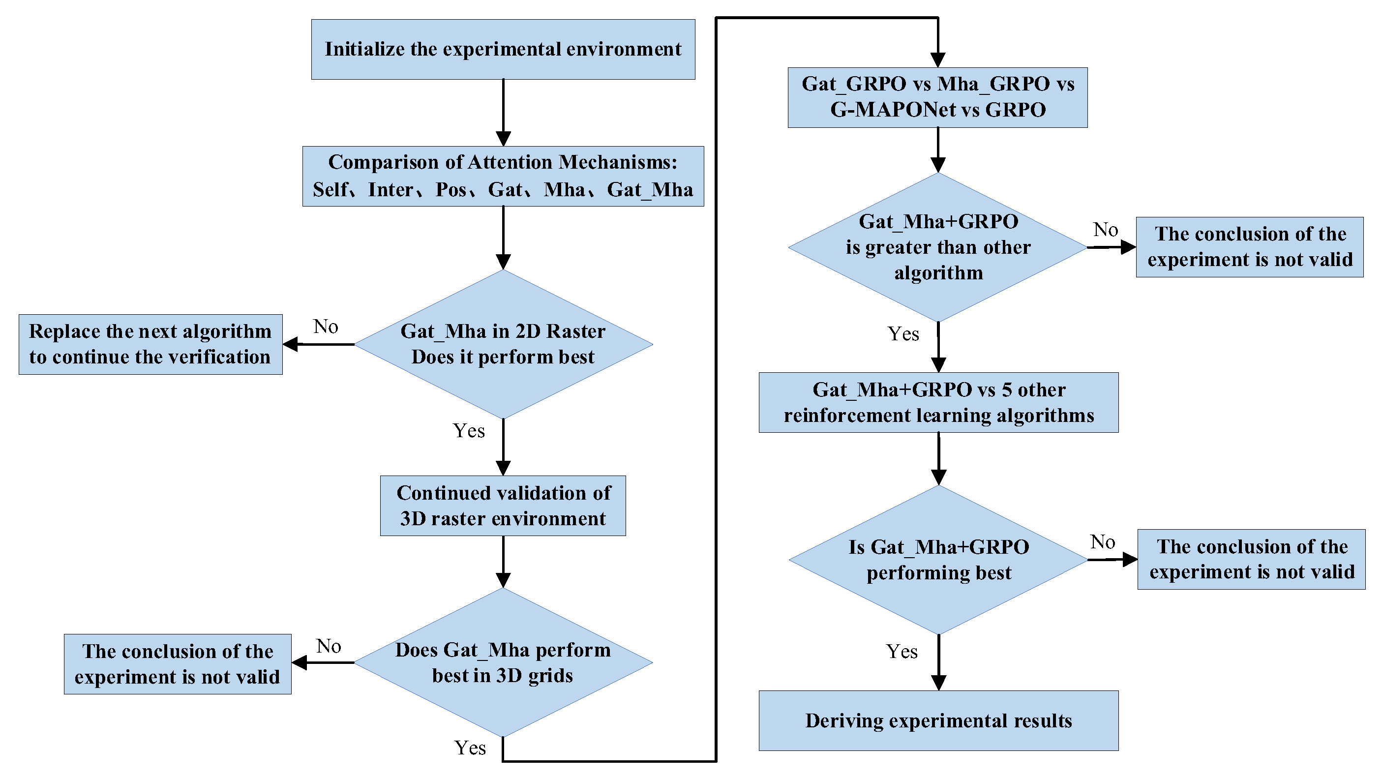
To validate the effectiveness of the G-MAPONet algorithm—which integrates a dual-layer attention mechanism with the GRPO framework for UAV dynamic trajectory planning in logistics—our experimental design combines simulation using the PyCharm platform (pycharm-community-2023.3) with real-world UAV flight tests. The evaluation comprises four comparative experimental setups, as illustrated in Figure 3. The procedures are summarized as follows:
  • Experiment 1 assesses both the objective function and constraint conditions of UAV delivery. The flight environment is constructed as a 7 × 7 two-dimensional obstacle map composed of a 7 × 7 grid of cells (each cell representing 100 m), using Matplotlib-3.7 within the PyCharm simulation environment. Several attention mechanisms—Self, Inter, Pos, Gat, Mha, and Gat_Mha—are implemented and compared.
  • Experiment 2 extends the environment to a 6 × 6 × 4 three-dimensional grid (each cell representing 100 m) to evaluate the robustness and generalizability of the results from Experiment 1. The same set of attention mechanisms is tested under this more complex spatial configuration to examine performance in higher-dimensional settings.
  • Experiment 3 conducts real-world flight validation based on the findings from the first two simulation experiments. A 1000 m × 1000 m × 120 m three-dimensional environment is employed, incorporating both the path planning and delivery constraints of UAV logistics. Four configurations are evaluated: the single-layer GRPO algorithm, the dual-layer GRPO-GAT architecture, the dual-layer GRPO-MHA architecture, and the three-layer G-MAPONet architecture.
  • Experiment 4 evaluates the timeliness and responsiveness of the three-layer G-MAPONet architecture in real-world delivery scenarios. It compares G-MAPONet with other reinforcement learning algorithms—GRPO, PPO, TRPO, A3C, and DQN—under identical experimental conditions.

3.2.2. Simulation Environment

Experiments on Different Attention Mechanisms in 2D Environments
To investigate the performance differences among different attention mechanisms in logistics UAVs, a 7 × 7 2D grid (each grid cell representing 100 m) was plotted using the Matplotlib tool on the PyCharm simulation platform, as shown in Figure 4. Among them, black areas represent obstacles, the top-left corner of the gray area is the starting point, and the bottom-right corner is the target endpoint. In the path planning process, Figure 4a, Inter Path Planning, and Figure 4b, Gat Path Planning, fell into detour and stagnation at the starting point; Figure 4c, Pos Path Planning, and Figure 4e, Mha Path Planning, encountered obstacles when planning the path to the lower area and fell into detour exploration; Figure 4d, Self Path Planning, encountered the boundary while moving along the rightward path and entered detour exploration; and Figure 4f, Gat_Mha Path Planning, which combines the advantages of Gat and Mha, initially explored from both sides to attempt to reach the target endpoint faster.
Experiments on Different Attention Mechanisms in 3D Environments
To conduct further experiments, the aforementioned 2D experimental environment is modified into a 6 × 6 × 4 3D grid environment (each grid cell representing 100 m), as shown in Figure 5. In the environment, black objects denote fixed obstacles, green objects represent moving obstacles, light blue circles indicate the starting position, pink circles mark the target end position, and yellow lines represent the UAV’s flight trajectory from the start to the target. The UAV performs path planning experiments by flying from the starting position at the bottom-left corner to the target at the top-right corner while avoiding obstacles. Comparative analysis demonstrates that the Gat_Mha attention mechanism exhibits superior capability in capturing and processing features of 3D spatial environments. It can avoid obstacles to a certain extent and successfully complete the navigation to the target end position. Although there is still room for optimization, it has already shown considerable potential in complex 3D scenarios.

3.2.3. Real Flight Environment

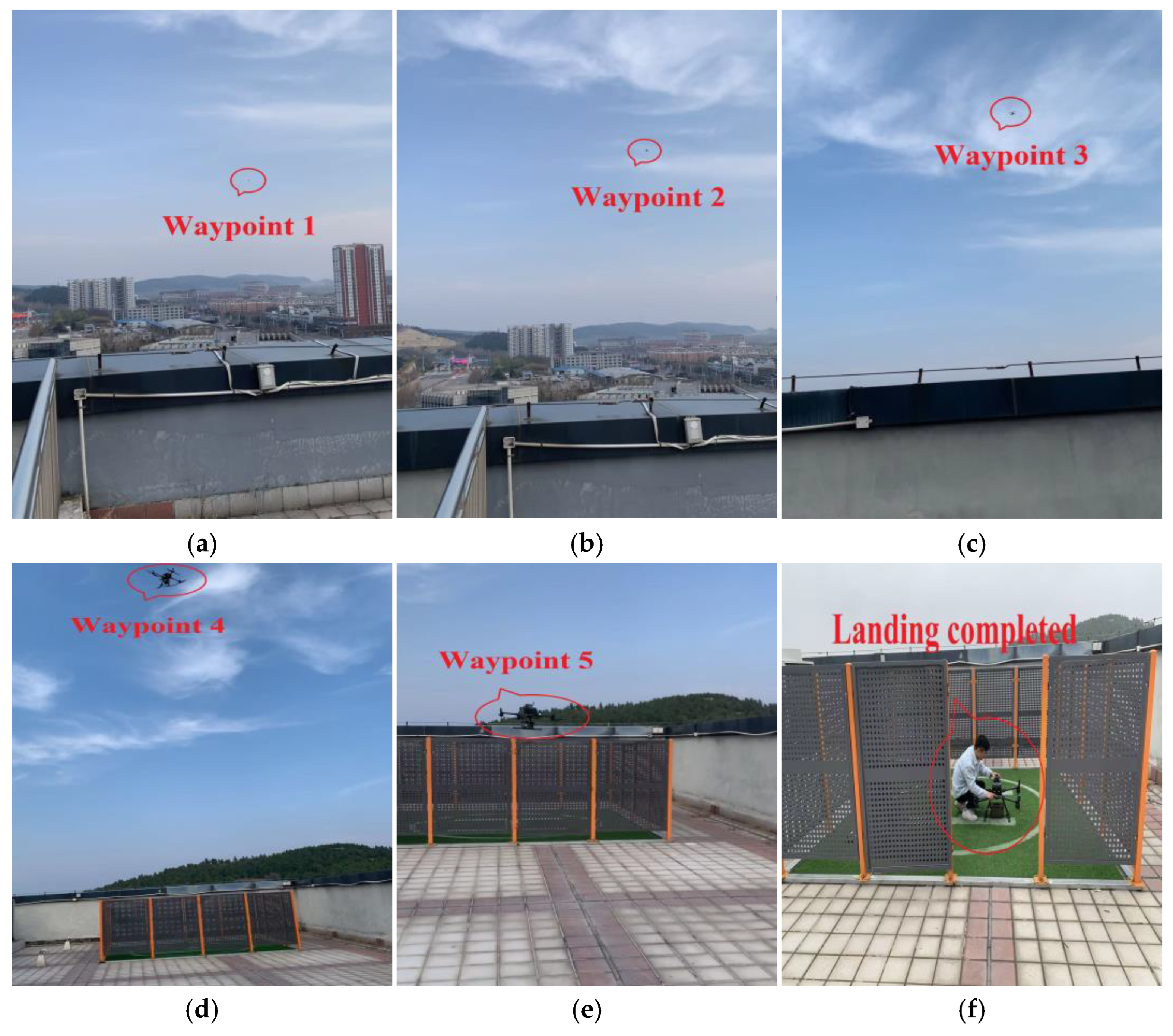
The actual flight experiment of the UAV is presented in Figure 6, conducted within a 1000 m × 1000 m × 120 m flight scenario. For this experiment, secondary development was performed on the DJI M350 UAV: the Jetson TX2 development board was employed as the host computer control center, configured with the Ubuntu 18.04 operating system and equipped with the ROS Melodic framework. This setup primarily handles large-volume data from multi-source sensors (including radar and vision), and generates trajectory paths by integrating the proposed algorithm. The closed-loop interaction process between the host computer and the M350 UAV is as follows: The Jetson TX2 receives sensor data (acquisition frequency: 20 Hz) returned by the M350 flight controller in real time via the serial port (configured with a communication baud rate of 115,200). After processing by the ROS Melodic node, trajectory control commands are generated, and the corresponding command frames are then sent to the M350 via the serial port. Meanwhile, a remote computer (configured with the same Ubuntu 18.04 + ROS Melodic environment as the Jetson TX2) establishes communication with the Jetson TX2 via SSH, enabling real-time monitoring of the experiment and online parameter debugging. To ensure communication reliability, this system adopts a standardized serial port data frame design: ① The sensor data frame (28 bytes in length) includes the frame header (0xAA), UAV pose (longitude, latitude, altitude), obstacle distance, battery level, and other key parameters, with a CRC16 check bit appended at the end to prevent data transmission errors; ② The control command frame (16 bytes in length) covers control information such as the frame header (0xBB), target waypoint coordinates, attitude adjustment value, and flight mode, which is also sent after CRC16 verification. The entire flight process involves the waypoint sequence shown in Figure 6a–f. The aforementioned interaction logic and data transmission specifications provide robust support for the stable execution of the experiment.
Ablation Study of the G-MAPONet Algorithm
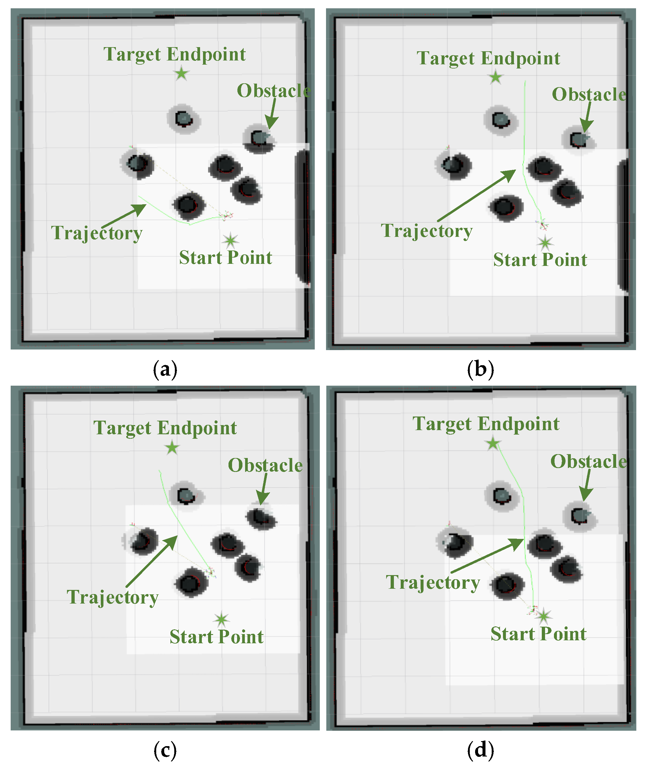
Figure 7 presents the results of the third UAV flight experiment. In this experiment, the Jetson TX2 development board mounted on the UAV was configured with PyTorch 1.9.1 and Python 3.8. A comparative evaluation was conducted using different path planning algorithms to navigate from the starting point to the destination. Specifically, Figure 7a illustrates the path generated by the GRPO algorithm, Figure 7b displays the GAT and GRPO fusion algorithm, Figure 7c shows the MHA and GRPO fusion algorithm, and Figure 7d presents the G-MAPONet algorithm; The GRPO model comprises three layers: an input layer with 64 dimensions, a hidden layer incorporating an activation function, and an output layer also with 64 dimensions. The training parameters include a learning rate of 0.001, a discount factor of 0.95, and a policy update pruning coefficient of 0.2; The Gat_GRPO and Mha_GRPO models adopt the same architectural configuration as GRPO, with the addition of 4 attention heads in each. In the G-MAPONet algorithm, both the GAT and MHA layers are configured with 4 attention heads.
Experiments on Different RL Algorithms
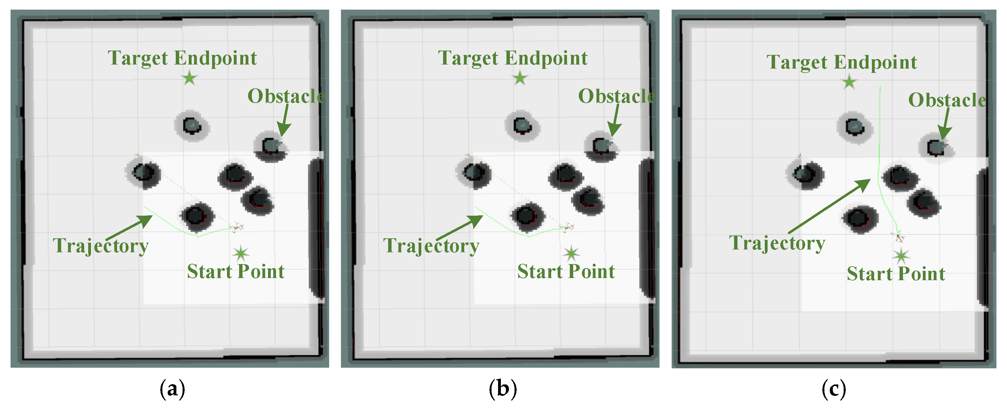
Figure 8 illustrates the actual flight environment experiment for the unmanned aerial vehicle. The starting point is located at the lower right corner, and the target point at the upper left corner, with multiple obstacles distributed in between. Path planning experiments were conducted using various algorithms, all starting from the lower right corner and ending at the upper left corner. Specifically, Figure 8a displays the results of the GRPO algorithm, Figure 8b those of the PPO algorithm, Figure 8c the TRPO algorithm, Figure 8d the A3C algorithm, Figure 8e the DQN algorithm, and Figure 8f the G-MAPONet algorithm. The GRPO algorithm adopts the same parameter settings as in Experiment 3, while the PPO, TRPO, A3C, and DQN algorithms employ identical parameters to ensure comparability.

3.3. Comparison Results of Different Attention Mechanisms

3.3.1. Experiments on Different Attention Mechanisms in 2D Training Environments

As shown in Figure 9 are the comparative training results of different attention mechanisms in the aforementioned 3D environment. From Figure 9a, the success rate of the Gat_Mha attention mechanism rises rapidly to approach 1.0 in the early stage of training, then maintains good robustness, and completes the layout planning of the optimal path trajectory in complex spaces. From Figure 9b,c, the average reward of Gat_Mha shows a more obvious improvement compared with other attention methods in the early training stage, being significantly superior to other attention mechanisms. In Figure 9d, the reward distribution of Gat_Mha is concentrated in the high-value region compared with other attention methods. This further indicates that the stability and effectiveness of the Gat_Mha attention mechanism strategy far exceed those of other mechanism methods, and it also exhibits significant advantages in the 3D grid environment.

3.3.2. Experiments on Different Attention Mechanisms in 3D Training

Figure 10 presents the results of the attention mechanism comparison in the three-dimensional environment. As shown in Figure 10a, the Gat_Mha attention mechanism achieves a rapid increase in success rate during early training, approaching 1.0, and maintains strong robustness while effectively completing optimal path trajectory planning in complex spaces. These results indicate that Gat_Mha significantly outperforms other methods in terms of strategy stability, effectiveness, and adaptability within three-dimensional grid environments.

3.4. Comparison Results of Different Reinforcement Learning Algorithms

3.4.1. Ablation Study of the G-MAPONet Algorithm in Training

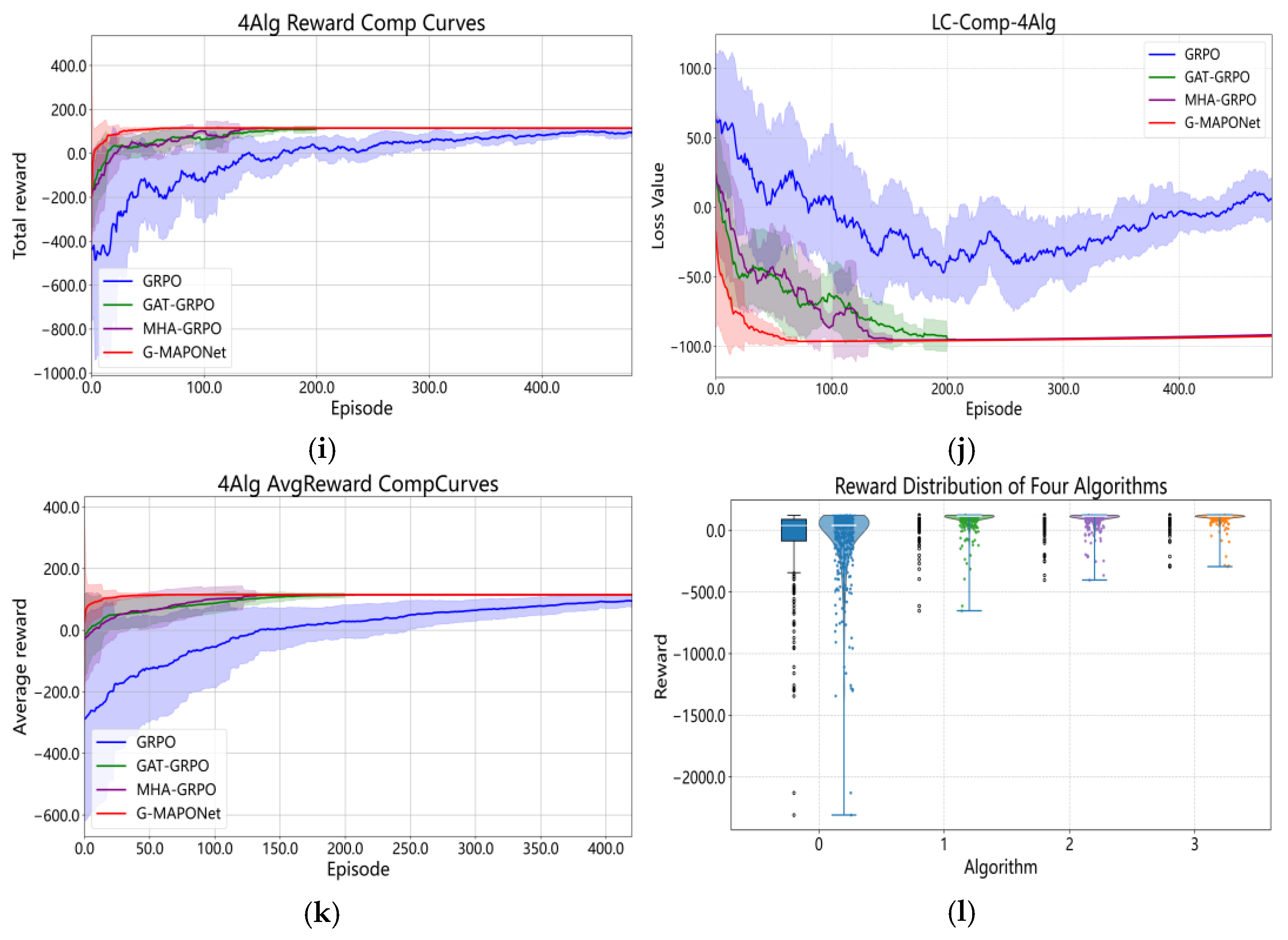
Figure 11 presents the training results of G-MAPONet in comparison with GRPO, Gat_GRPO, and Mha_GRPO. As illustrated in Figure 11a,e,i, G-MAPONet achieves a rapid increase in total reward, stabilizing near 100, whereas GRPO shows a slower rise and becomes negative at 100 training iterations. This highlights G-MAPONet’s superior reward acquisition and overall performance. Figure 11b,f,j demonstrate that G-MAPONet’s loss decreases quickly and stabilizes, while GRPO exhibits significant fluctuations and looping behavior, indicating a more efficient and stable optimization strategy in G-MAPONet. From Figure 11c,g,k, it is evident that G-MAPONet maintains a consistently high average reward, outperforming GRPO and reinforcing its strategic advantage. Finally, as shown in Figure 11d,h,l, G-MAPONet’s rewards are predominantly concentrated in the high-value range, whereas GRPO’s rewards are more dispersed and mainly located in low-value regions with greater data variability. These findings further validate G-MAPONet’s improved convergence and effectiveness in generating high-quality trajectory strategies.

3.4.2. Experiments on Different RL Algorithms in Training

Figure 12 presents the training results of G-MAPONET in comparison with GRPO, PPO, TRPO, A3C, and DQN reinforcement learning algorithms. As illustrated in Figure 12a,e,i, G-MAPONET achieves a significantly higher total reward than all other algorithms, particularly DQN and TRPO, which exhibit substantial fluctuations. Figure 12b,f,j demonstrate that G-MAPONET’s loss decreases rapidly and stabilizes, whereas the other algorithms display varying degrees of instability, with DQN showing particularly large amplitude oscillations. From Figure 12c,g,k, it is evident that G-MAPONET consistently maintains a high average reward, outperforming all competing methods. Notably, the TRPO algorithm exhibits persistent fluctuations and signs of non-convergence, highlighting its limitations in stable learning. These findings further support G-MAPONET’s superior capability in strategy optimization, enabling the consistent generation of high-quality trajectory paths. Finally, as shown in Figure 12d,h,l, G-MAPONET’s reward distribution is predominantly concentrated in the high-value range, confirming its enhanced effectiveness, reward acquisition, and convergence performance in trajectory planning.

4. Discussion

4.1. Analysis of Experimental Data in Reinforcement Learning

This section provides a concise summary and comprehensive analysis of the results obtained from the previous experiments. To enhance clarity, the following abbreviations are employed: Path Planning Task Completion Status (PPTC), Number of Convergence Episodes (NCE), Path Planning Length (PPL), Episode (NE), and Average Reward (AR). In the experiment, the parameters of the G-MAPONet algorithm are configured as follows: the embedding dimension of features is set to 64; the number of heads in the multi-head attention mechanism is set to 4; the learning rate of the policy network is set to 0.001; the learning rate of the value network is set to 0.001; the coefficient for controlling the policy update magnitude is set to 0.2; and the interval number of episodes for evaluating training performance is set to 100.

4.1.1. Discussion on the Ablation Study of the G-MAPONet Algorithm

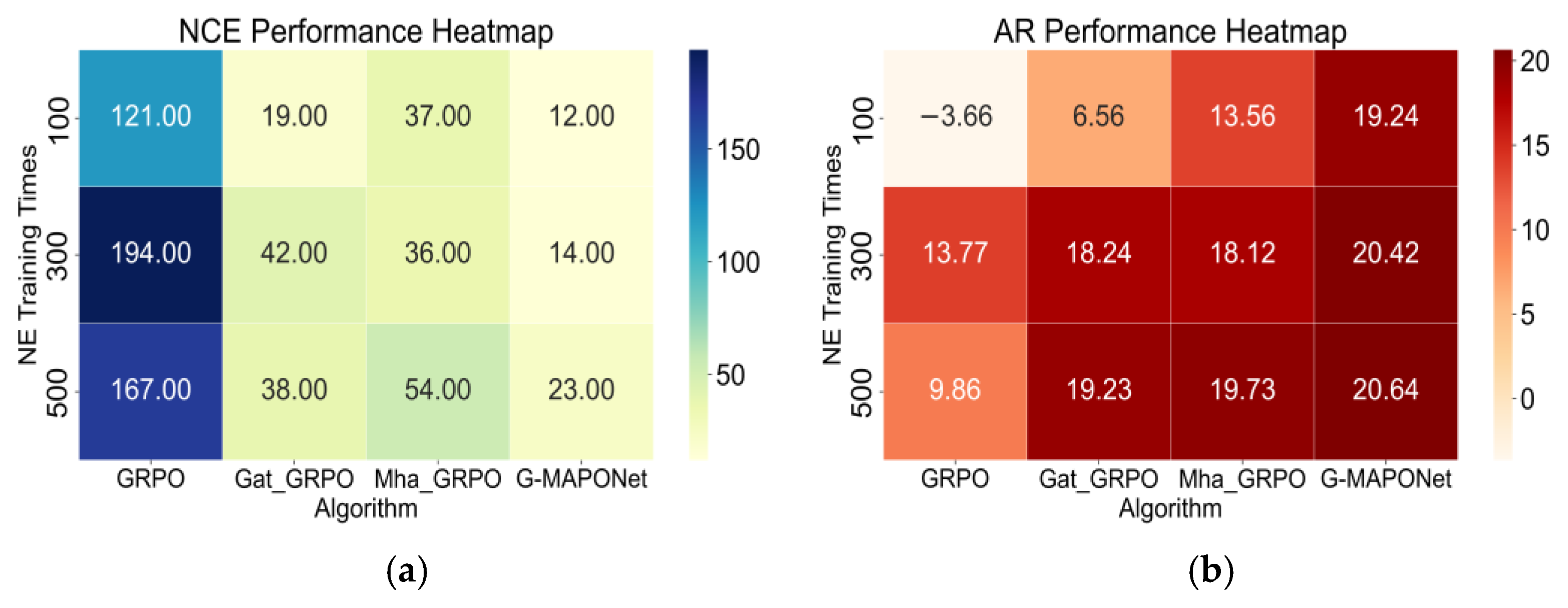
The data for the above experiment three using the GRPO algorithm, Gat_GRPO algorithm, Mha_GRPO algorithm and G-MAPONet algorithm are shown in Table 1.
Table 1 presents a comparative analysis of the NCE, AR, and PPTC indicators across different attention mechanisms, with results illustrated in Figure 13. In the context of dynamic trajectory planning, Figure 13a demonstrates that the GPRO algorithm failed to converge within 100 training iterations, whereas the improved Gat_GRPO, Mha_GRPO, and G-MAPONet algorithms all achieved convergence. Specifically, across 100, 300, and 500 iterations, the average convergence rate of Gat_GRPO was 79.96% higher than that of GPRO; Mha_GRPO was 72.84% higher; and G-MAPONet was 89.70% higher. As shown in Figure 13b, the average reward values of Gat_GRPO, Mha_GRPO, and G-MAPONet consistently exceeded those of GPRO across all three training rounds. These findings provide strong evidence that the improved G-MAPONet algorithm significantly enhances the performance of GRPO, demonstrating faster convergence and greater robustness under identical training conditions.

4.1.2. Discussion on the Results of Different RL Algorithms

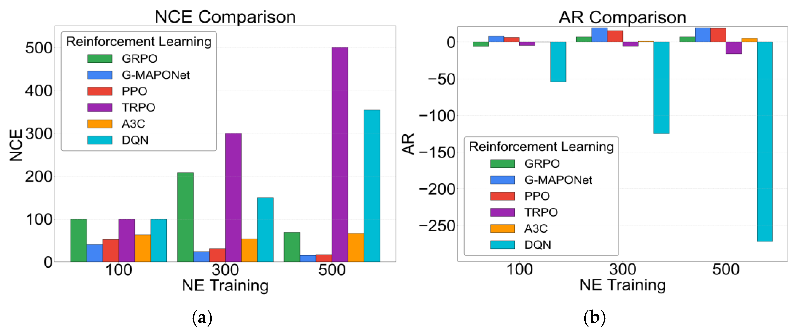
Building on the superior performance of the G-MAPONet algorithm observed in Experiment 3, further experiments were carried out using the PPO, TRPO, A3C, and DQN algorithms to rigorously validate the hypothesis. The experimental results are summarized in Table 2.
Table 2 presents a comparative analysis of the NCE, AR, and PPTC metrics across various reinforcement learning algorithms, with results illustrated in Figure 14. As shown in Figure 14a, G-MAPONet demonstrates superior convergence performance compared to other algorithms at NE values of 100, 300, and 500 training rounds. Specifically, compared to the best-performing PPO algorithm, G-MAPONet reduces convergence rounds by 23.08%, 22.58%, and 11.76% at NE = 100, 300, and 500, respectively, yielding an average reduction of 19.14%. In terms of average reward (AR) as shown in Figure 14b, G-MAPONet outperforms PPO by 21.86%, 24.24%, and 2.50% at the same NE values, resulting in an overall improvement of 16.20%. Regarding PPTC, G-MAPONet successfully completes dynamic path planning across all NE values, whereas PPO, GRPO, and A3C only succeed at NE = 300 and 500, and TRPO fail in all training rounds. Overall, G-MAPONet consistently outperforms GRPO, PPO, TRPO, A3C, and DQN across all three evaluation metrics, providing strong evidence of its superior performance and robustness in logistics UAV path planning.

4.2. Comparison of RL Algorithms Under the APF Benchmark Function

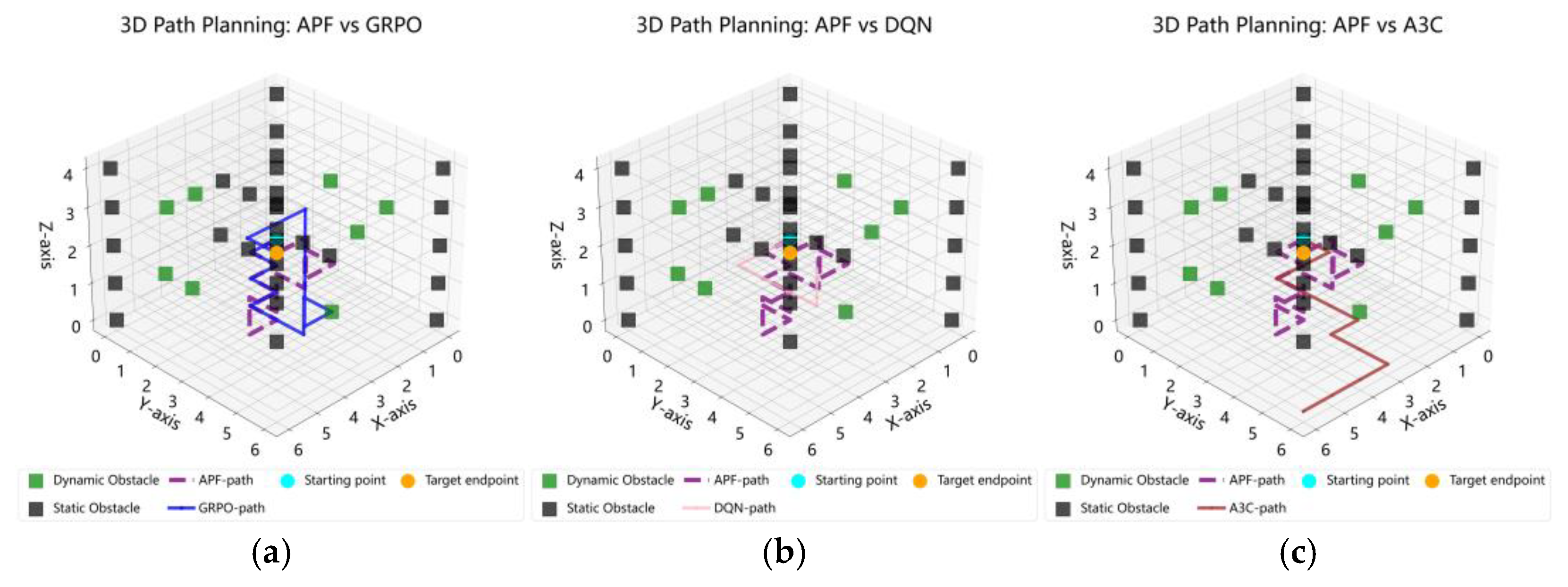
To further verify the trajectory planning performance of various reinforcement learning algorithms, the APF heuristic algorithm is introduced as a benchmark to compare these reinforcement learning algorithms. The trajectory comparisons between each reinforcement learning algorithm and the benchmark APF heuristic algorithm are shown in Figure 15.
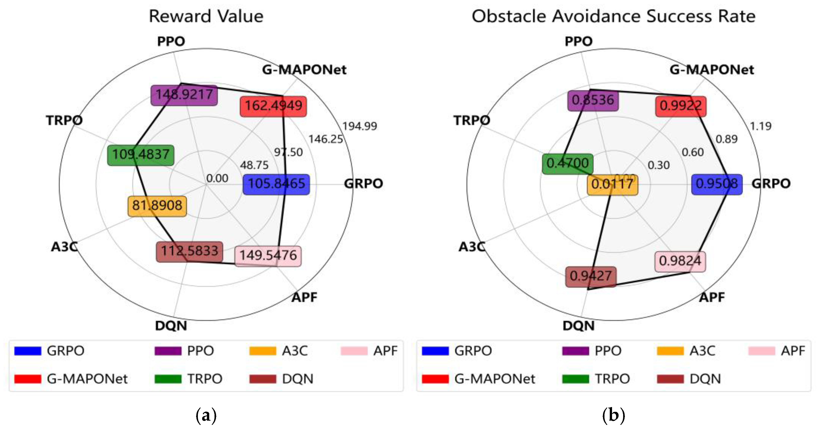
From the comparisons between various reinforcement learning algorithms and the benchmark heuristic trajectory in Figure 16 above, the final reward value and obstacle avoidance success rate are used as key comparison metrics, and the conclusions drawn are shown in Figure 16 and Table 3.
As can be seen from the data in Table 3 above, after 500 iterations, the final reward value and obstacle avoidance success rate of the improved G-MAPONet algorithm are significantly higher than those of other algorithms. Compared with the benchmark APF, it achieves an 8.66% improvement in the final reward value and also shows an enhancement in the obstacle avoidance repetition rate, which further verifies the effectiveness of the improved G-MAPONet algorithm.

5. Conclusions

Through the designed objective function and multiple constraints, extensive path planning experiments demonstrate that the Gat_Mha attention mechanism outperforms other attention mechanisms. By integrating the GAT, MHA, and GRPO layers, the three-layer G-MAPONet algorithm is constructed. The key findings are summarized as follows:
(1)
Compared with Self, Inter, Pos, Gat, and Mha attention mechanisms, the fused Gat_Mha mechanism shows superior performance in On-Time Completion Rate and Total Training Convergence Time. Moreover, the Path Planning Task Completion Status is fully achieved, indicating enhanced capabilities in environmental feature modeling and path planning.
(2)
When comparing GRPO with the improved Gat_GRPO, Mha_GRPO, and G-MAPONet algorithms, the results show that G-MAPONet achieves the highest performance. Specifically, in terms of NCE, the convergence mean of Gat_GRPO improves by 79.96% over GPRO, Mha_GRPO by 72.84%, and G-MAPONet by 89.70%. In Average Reward (AR), the improved algorithms consistently outperform GPRO across all three training rounds. These results confirm that G-MAPONet offers the best convergence speed and robustness.
(3)
Further validation with GRPO, PPO, TRPO, A3C, and DQN reinforcement learning algorithms demonstrates that G-MAPONet significantly reduces the Number of Convergence Epochs (NCE). At NE = 100, 300, and 500, convergence rounds are reduced by 23.08%, 22.58%, and 11.76%, respectively, with an average reduction of 19.14%. In AR performance, G-MAPONet outperforms PPO—the best among the five—by 21.86%, 24.24%, and 2.50% at the same NE values, resulting in an overall improvement of 16.20%. Regarding PPTC, G-MAPONet successfully completes dynamic planning at all NE values, demonstrating excellent stability and generalization. In contrast, PPO, GRPO, and A3C succeed only at NE = 300 and 500, while DQN and TRPO fail in all sessions, highlighting limitations in adaptability and state decoupling.
(4)
Finally, the APF heuristic algorithm is added as a baseline. After 500 iterations, the results indicate that the reward values and obstacle avoidance success rate of G-MAPONet are significantly higher than those of other algorithms. Compared with the baseline APF, the reward values are improved by 8.66%, and the obstacle avoidance repetition rate is also enhanced. This further verifies the effectiveness of the improved G-MAPONet algorithm.
In summary, G-MAPONet provides an effective solution for logistics UAV dynamic path planning, characterized by efficient training, high-quality trajectory generation, and stable task execution. This confirms its strong performance and robustness in complex environments.
Despite its current advantages, future research can focus on four directions:
(1)
Optimizing the algorithm architecture by refining feature modeling and exploring dynamic adaptive fusion strategies between GAT and MHA layers to enhance adaptability to complex environments.
(2)
Extending algorithm robustness to unstructured environments with dynamic obstacles.
(3)
Developing multi-UAV cooperative planning to improve task allocation and coordination among agents, enhancing group efficiency and safety.
(4)
Investigating the theoretical foundation of the GAT-MHA attention mechanism in diverse application scenarios to provide stronger theoretical support for strategy optimization.
These future improvements will further enhance the algorithm’s performance and practical value, advancing the development of trajectory planning technologies for UAVs.

Author Contributions

J.D.: Conceptualization, Investigation, Validation, Writing—original draft, Writing—review & editing, Formal analysis, Data curation, Investigation. Y.Z.: Formal analysis, Data curation, Investigation, Project administration, Writing—original draft. M.H.: Methodology, Visualization, Investigation, Supervision, Writing—review & editing. Y.S.: Data curation, Investigation, Project administration. H.Z.: Conceptualization, Funding acquisition, Supervision, Writing—review & editing. All authors have read and agreed to the published version of the manuscript.

Funding

This study was supported by The National Social Science Fund of China (No. 22&ZD169) and The Key project of Civil Aviation Joint Fund of National Natural Science Foundation of China (No. U2133207).

Data Availability Statement

The original contributions presented in this study are included in the article. Further inquiries can be directed to the corresponding author.

Conflicts of Interest

The authors declare no conflicts of interest.

Abbreviations

G-MAPONetGraph Multi-Head Attention Policy Optimization Network
PPTCPath Planning Task Completion Status
NCENumber of Convergence Episodes
PPLPath Planning Length
NEEpisode
ARAverage Reward
GRPOGroup Relative Policy Optimization
CVRPCapacitated Vehicle Routing Problem
PSOParticle Swarm Optimization
C-SPPOCentralized-S Proximal Policy Optimization
MARLMulti-Agent Reinforcement Learning
RLReinforcement Learning
RRT*Rapidly Exploring Random Tree Star
SARSAState-Action-Reward-State-Action
MPCModel Predictive Control
DQNDeep Q-Network
ACO-DQN-TPAnt Colony Optimization–Deep Q-Network–Time Parameter
PO-WMFDDPGPartially Observable Weighted Mean Field Reinforcement Learning
GAT-RLGraph Attention Networks–Reinforcement Learning
MTCRMaximum timeliness compliance rate
MECMinimum energy consumption
FRVFinal Reward Value
OASRObstacle Avoidance Success Rate

Appendix A

All variables and symbols in the text are defined as shown in Table A1.
Table A1. Parameter setting.
ParameterMeaning
W m Attention head weight matrix
α m Attention score parameter vector
α gat m The attention parameter vector of the m-th GAT attention head
d h Dimension of the hidden layer
d f Dimension of input features
M Total number of attention heads
m Number of attention heads
W gat m Weight matrix of the m-th attention head in the GAT model
C Constant
H 0 Initial feature matrix input to GAT
i ,   j Node
H m Feature matrix transformed by the m attention head of GAT
H m [ i ] In the m-th attention head of GAT, the feature vector of node i after feature transformation
H m [ j ] In the m-th attention head of GAT, the feature vector of node j after feature transformation
e i , j , m Attention score between node i and node j under the m-th attention head
e i , w , m The unnormalized attention score between node i and domain node ω
W i , j , m Normalized attention weight of node i for neighbor node j under the m-th attention head
h i , m The new feature representation of node i under the m-th attention head, obtained after weighted aggregation of neighbor features
M gat Number of attention heads in GAT
Z gat The final node feature matrix output by the GAT model
x Input value of nonlinear feature
ξ Input of the current batch of data
T Target value
λ Regularization coefficient
Γ Loss value of the total batches
Γ b Loss values of the current batch data
Θ The set of all parameters learned by the model
  h Number of heads in the multi-head attention mechanism
d model Feature dimension of the model
X b Input feature matrix for each batch
Q Query matrix
K Key matrix
V Value matrix
Q K T Calculate the dot product of the query matrix and the key matrix
Z h Matrix after multi-head attention concatenation
Z Model final output feature matrix
  γ Learning rate
  W Q Query weight matrix
W K Key weight matrix
W V Value weight matrix
W O Output weight matrix
  σ Noise figure
  a t UAV performs an action at time t
  r t After performing action a t at time t, the immediate reward obtained by the drone from the environment
s t Fusing information from different subspaces into the output of multi-head attention
  s t + 1 At   time   t ,   performing   action     a t leads to the environment transitioning to the next state
( 0 , I ) Standard Gaussian distribution
  δ t Value   network   at   time   t   state     s t value estimate
done Boolean value indicating whether the cyclic task has ended
done t Termination flag
V [ t ] Measuring the advantage of taking a certain action at time t relative to the average policy
l Generalized advantage estimation parameter, with a range of values between (0,1), used to dynamically balance the bias and variance fluctuation range
  A Advantage function
  mean ( A ) Mean of A
  std ( A ) Standard deviation of A
  π θ Updated policy
r ( θ ) Importance sampling ratio
s batch State representation in a batch of data
a batch In   state   s batch , the action actually executed
A batch Advantage values corresponding to batch data
  J ( θ ) Objective function of the policy’s expected return
  θ Parameters   of   the   policy   function     π θ
E [ ] Expectation
  ε Discount factor
  J Gradient vector
  π old Old policy
  π new New policy
  δ Preset trust region value
  η Step size backoff coefficient
r batch Immediate reward of the batch data
y batch Target value of the value network for the batch
s t + 1 Next state
V φ ( s t + 1 ) Value estimation of the next state by the value network
done batch Termination flag of the batch data
V φ Value network
B Batch size
L V Loss function of the value network
φ Parameters of the value network
L V Gradient   of   the   Loss   Function   L V with Respect to Value Network Parameters φ
θ old Parameters of the old policy network
p 0 Logistics distribution center
p i , k The k-th node in the delivery path of the i-th UAV
ϑ i , k The load of the i-th UAV at the k-th node
ϑ i , n i The   load   at   the   delivery   node   n i of the i-th UAV
ρ Energy consumption coefficient per unit load distance
v i UAV flight speed
TT i , j The load at the delivery node j of the i-th UAV
zz i , j The height of the i-th route flying to the j-th track point relative to sea level
hh r , max Relative flight altitude
hh a , max Maximum absolute altitude of flight
HH i , j Actual flight altitude at the j-th waypoint of the i-th route
G Total takeoff weight
ff d Drag coefficient
FF max Maximum limit of total flight thrust
v min Minimum flying speed
v max Maximum flight speed
T max Maximum Flight Time
ς Height coefficient, range of values (0,1)

References

  1. Rascon Enriquez, J.; Castillo-Toledo, B.; Di Gennaro, S.; García-Delgado, L.A. An algorithm for dynamic obstacle avoidance applied to UAVs. Robot. Auton. Syst. 2025, 186, 104907. [Google Scholar] [CrossRef]
  2. Dukkanci, O.; Koberstein, A.; Kara, B.Y. Drones for relief logistics under uncertainty after an earthquake. Eur. J. Oper. Res. 2023, 310, 117–132. [Google Scholar] [CrossRef]
  3. Jin, Z.; Ng, K.K.H.; Zhang, C.; Chan, Y.Y.; Qin, Y. A multistage stochastic programming approach for drone-supported last-mile humanitarian logistics system planning. Adv. Eng. Inform. 2025, 65, 103201. [Google Scholar] [CrossRef]
  4. Hu, C.; Li, Y.; Qu, G. Integrated dynamic task allocation via event-triggered for tracking ground moving targets by UAVs in urban. Robot. Auton. Syst. 2025, 193, 105061. [Google Scholar] [CrossRef]
  5. Sun, Q.; Liu, W.; Cai, L. Multi-dynamic target coverage tracking control strategy based on multi-UAV collaboration. Control Eng. Pract. 2025, 155, 106170. [Google Scholar] [CrossRef]
  6. Dudek, T.; Kaśkosz, K. Optimizing drone logistics in complex urban industrial infrastructure. Transp. Res. Part D Transp. Environ. 2025, 140, 104610. [Google Scholar] [CrossRef]
  7. Li, S.; Zhang, H.; Yi, J.; Liu, H. A bi-level planning approach of logistics unmanned aerial vehicle route network. Aerosp. Sci. Technol. 2023, 141, 108572. [Google Scholar] [CrossRef]
  8. Abualola, H.; Mizouni, R.; Otrok, H.; Singh, S.; Barada, H. A matching game-based crowdsourcing framework for last-mile delivery: Ground-vehicles and Unmanned-Aerial Vehicles. J. Netw. Comput. Appl. 2023, 213, 103601. [Google Scholar] [CrossRef]
  9. Moshref-Javadi, M.; Hemmati, A.; Winkenbach, M. A truck and drones model for last-mile delivery: A mathematical model and heuristic approach. Appl. Math. Model. 2020, 80, 290–318. [Google Scholar] [CrossRef]
  10. Pang, S.; Chai, Q.; Liu, N.; Zheng, W. A multi-objective cat swarm optimization algorithm based on two-archive mechanism for UAV 3-D path planning problem. Appl. Soft Comput. 2024, 167, 112306. [Google Scholar] [CrossRef]
  11. Shen, Q.; Zhang, D.; He, Q.; Ban, Y.; Zuo, F. A novel multi-objective dung beetle optimizer for Multi-UAV cooperative path planning. Heliyon 2024, 10, e37286. [Google Scholar] [CrossRef]
  12. Goel, U.; Varshney, S.; Jain, A.; Maheshwari, S.; Shukla, A. Three Dimensional Path Planning for UAVs in Dynamic Environment using Glow-worm Swarm Optimization. Procedia Comput. Sci. 2018, 133, 230–239. [Google Scholar] [CrossRef]
  13. Chowdhury, A.; De, D. RGSO-UAV: Reverse Glowworm Swarm Optimization inspired UAV path-planning in a 3D dynamic environment. Ad. Hoc Netw. 2023, 140, 103068. [Google Scholar] [CrossRef]
  14. Bashir, N.; Boudjit, S.; Dauphin, G.; Zeadally, S. An obstacle avoidance approach for UAV path planning. Simul. Model. Pract. Theory 2023, 129, 102815. [Google Scholar] [CrossRef]
  15. Boulares, M.; Barnawi, A. A novel UAV path planning algorithm to search for floating objects on the ocean surface based on object’s trajectory prediction by regression. Robot. Auton. Syst. 2021, 135, 103673. [Google Scholar] [CrossRef]
  16. Freitas, H.; Faiçal, B.S.; Cardoso E Silva, A.V.; Ueyama, J. Use of UAVs for an efficient capsule distribution and smart path planning for biological pest control. Comput. Electron. Agr. 2020, 173, 105387. [Google Scholar] [CrossRef]
  17. Du, P.; He, X.; Cao, H.; Garg, S.; Kaddoum, G.; Hassan, M.M. AI-based energy-efficient path planning of multiple logistics UAVs in intelligent transportation systems. Comput. Commun. 2023, 207, 46–55. [Google Scholar] [CrossRef]
  18. Guo, C.; Huang, L.; Tian, K. Combinatorial optimization for UAV swarm path planning and task assignment in multi-obstacle battlefield environment. Appl. Soft Comput. 2025, 171, 112773. [Google Scholar] [CrossRef]
  19. Wang, X.; Gao, X.; Wang, L.; Su, X.; Jin, J.; Liu, X.; Deng, Z. Resilient multi-objective mission planning for UAV formation: A unified framework integrating task pre- and re-assignment. Def. Technol. 2025, 45, 203–226. [Google Scholar] [CrossRef]
  20. Escribano Macias, J.; Angeloudis, P.; Ochieng, W. Optimal hub selection for rapid medical deliveries using unmanned aerial vehicles. Transp. Res. Part C Emerg. Technol. 2020, 110, 56–80. [Google Scholar] [CrossRef]
  21. Khan, S.I.; Qadir, Z.; Munawar, H.S.; Nayak, S.R.; Budati, A.K.; Verma, K.D.; Prakash, D. UAVs path planning architecture for effective medical emergency response in future networks. Phys. Commun-Amst. 2021, 47, 101337. [Google Scholar] [CrossRef]
  22. Xiao, J.; Yuan, G.; Xue, Y.; He, J.; Wang, Y.; Zou, Y.; Wang, Z. A deep reinforcement learning based distributed multi-UAV dynamic area coverage algorithm for complex environment. Neurocomputing 2024, 595, 127904. [Google Scholar] [CrossRef]
  23. Wang, F.; Zhang, H.; Du, S.; Hua, M.; Zhong, G. C-SPPO: A deep reinforcement learning framework for large-scale dynamic logistics UAV routing problem. Chin. J. Aeronaut. 2025, 38, 103229. [Google Scholar] [CrossRef]
  24. Brotee, S.; Kabir, F.; Razzaque, M.A.; Roy, P.; Mamun-Or-Rashid, M.; Hassan, M.R.; Hassan, M.M. Optimizing UAV-UGV coalition operations: A hybrid clustering and multi-agent reinforcement learning approach for path planning in obstructed environment. Ad. Hoc Netw. 2024, 160, 103519. [Google Scholar] [CrossRef]
  25. Lee, M.H.; Moon, J. Deep reinforcement learning-based model-free path planning and collision avoidance for UAVs: A soft actor–critic with hindsight experience replay approach. ICT Express 2023, 9, 403–408. [Google Scholar] [CrossRef]
  26. Shamsoshoara, A.; Lotfi, F.; Mousavi, S.; Afghah, F.; Güvenç, I. Joint path planning and power allocation of a cellular-connected UAV using apprenticeship learning via deep inverse reinforcement learning. Comput. Netw. 2024, 254, 110789. [Google Scholar] [CrossRef]
  27. Bo, L.; Zhang, T.; Zhang, H.; Hong, J.; Liu, M.; Zhang, C.; Liu, B. 3D UAV path planning in unknown environment: A transfer reinforcement learning method based on low-rank adaption. Adv. Eng. Inform. 2024, 62, 102920. [Google Scholar] [CrossRef]
  28. Huang, S.; Chen, W.; Lu, B.; Xiao, F.; Shen, C.; Zhang, W. An improved BAT algorithm for collaborative dynamic target tracking and path planning of multiple UAV. Comput. Electr. Eng. 2024, 118, 109340. [Google Scholar] [CrossRef]
  29. Qu, C.; Gai, W.; Zhong, M.; Zhang, J. A novel reinforcement learning based grey wolf optimizer algorithm for unmanned aerial vehicles (UAVs) path planning. Appl. Soft Comput. 2020, 89, 106099. [Google Scholar] [CrossRef]
  30. Zhang, P.; Mei, Y.; Wang, H.; Wang, W.; Liu, J. Collision-free trajectory planning for UAVs based on sequential convex programming. Aerosp. Sci. Technol. 2024, 152, 109404. [Google Scholar] [CrossRef]
  31. Li, H.; Miao, F.; Mei, X. Facilitating Multi-UAVs application for rescue in complex 3D sea wind offshore environment: A scalable Multi-UAVs collaborative path planning method based on improved coatis optimization algorithm. Ocean. Eng. 2025, 324, 120701. [Google Scholar] [CrossRef]
  32. Aslan, M.F.; Durdu, A.; Sabanci, K. Goal distance-based UAV path planning approach, path optimization and learning-based path estimation: GDRRT, PSO-GDRRT and BiLSTM-PSO-GDRRT. Appl. Soft Comput. 2023, 137, 110156. [Google Scholar] [CrossRef]
  33. Swain, S.; Khilar, P.M.; Senapati, B.R. A reinforcement learning-based cluster routing scheme with dynamic path planning for mutli-UAV network. Veh. Commun. 2023, 41, 100605. [Google Scholar] [CrossRef]
  34. Zhang, Y.; Ding, M.; Yuan, Y.; Zhang, J.; Yang, Q.; Shi, G.; Jiang, J. Large-scale UAV swarm path planning based on mean-field reinforcement learning. Chin. J. Aeronaut. 2025, 38, 103484. [Google Scholar] [CrossRef]
  35. Deniz, N.; Jorquera, F.; Torres-Torriti, M.; Cheein, F.A. Model predictive path-following controller for Generalised N-Trailer vehicles with noisy sensors and disturbances. Control Eng. Pract. 2024, 142, 105747. [Google Scholar] [CrossRef]
  36. Chen, Y.; Xu, Y.; Yang, L.; Hu, M. In-flight fast conflict-free trajectory re-planning considering UAV position uncertainty and energy consumption. Transp. Res. Part C Emerg. Technol. 2025, 171, 104988. [Google Scholar] [CrossRef]
  37. Poudel, S.; Moh, S. Priority-aware task assignment and path planning for efficient and load-balanced multi-UAV operation. Veh. Commun. 2023, 42, 100633. [Google Scholar] [CrossRef]
  38. Sha, H.; Guo, R.; Zhou, J.; Zhu, X.; Ji, J.; Miao, Z. Reinforcement learning-based robust formation control for Multi-UAV systems with switching communication topologies. Neurocomputing 2025, 611, 128591. [Google Scholar] [CrossRef]
  39. Boulares, M.; Fehri, A.; Jemni, M. UAV path planning algorithm based on Deep Q-Learning to search for a floating lost target in the ocean. Robot. Auton. Syst. 2024, 179, 104730. [Google Scholar] [CrossRef]
  40. Liu, Z.; Li, L.; Zhang, X.; Tang, W.; Yang, Z.; Yang, X. Considering both energy effectiveness and flight safety in UAV trajectory planning for intelligent logistics. Veh. Commun. 2025, 52, 100885. [Google Scholar] [CrossRef]
  41. Zhao, B.; Huo, M.; Li, Z.; Yu, Z.; Qi, N. Clustering-based hyper-heuristic algorithm for multi-region coverage path planning of heterogeneous UAVs. Neurocomputing 2024, 610, 128528. [Google Scholar] [CrossRef]
  42. Liu, H.; Long, X.; Li, Y.; Yan, J.; Li, M.; Chen, C.; Gu, F.; Pu, H.; Luo, J. Adaptive multi-UAV cooperative path planning based on novel rotation artificial potential fields. Knowl.-Based Syst. 2025, 317, 113429. [Google Scholar] [CrossRef]
  43. Hu, X.; Yang, C.; Zhou, J.; Zhang, Y.; Ma, Y. Research on 3D layered visibility graph route network model and multi-objective path planning for UAVs in complex urban environments. Aerosp. Sci. Technol. 2025, 159, 109947. [Google Scholar] [CrossRef]
  44. Xu, X.; Xie, C.; Ma, L.; Yang, L.; Zhang, T. Multi-objective evolutionary algorithm with two balancing mechanisms for heterogeneous UAV swarm path planning. Appl. Soft Comput. 2025, 173, 112927. [Google Scholar] [CrossRef]
  45. Peng, Y.; Tan, G.; Si, H.; Li, J. DRL-GAT-SA: Deep reinforcement learning for autonomous driving planning based on graph attention networks and simplex architecture. J. Syst. Archit. 2022, 126, 102505. [Google Scholar] [CrossRef]
  46. Wang, W.; Li, X.; Tian, J. UAV formation path planning for mountainous forest terrain utilizing an artificial rabbit optimizer incorporating reinforcement learning and thermal conduction search strategies. Adv. Eng. Inform. 2024, 62, 102947. [Google Scholar] [CrossRef]
  47. Gao, J.; Jia, L.; Kuang, M.; Shi, H.; Zhu, J. An End-to-End Solution for Large-Scale Multi-UAV Mission Path Planning. Drones 2025, 9, 418. [Google Scholar] [CrossRef]
  48. Shukla, P.; Shukla, S.; Kumar Singh, A. Trajectory-Prediction Techniques for Unmanned Aerial Vehicles (UAVs): A Comprehensive Survey. IEEE Commun. Surv. Tutor. 2025, 27, 1867–1910. [Google Scholar] [CrossRef]
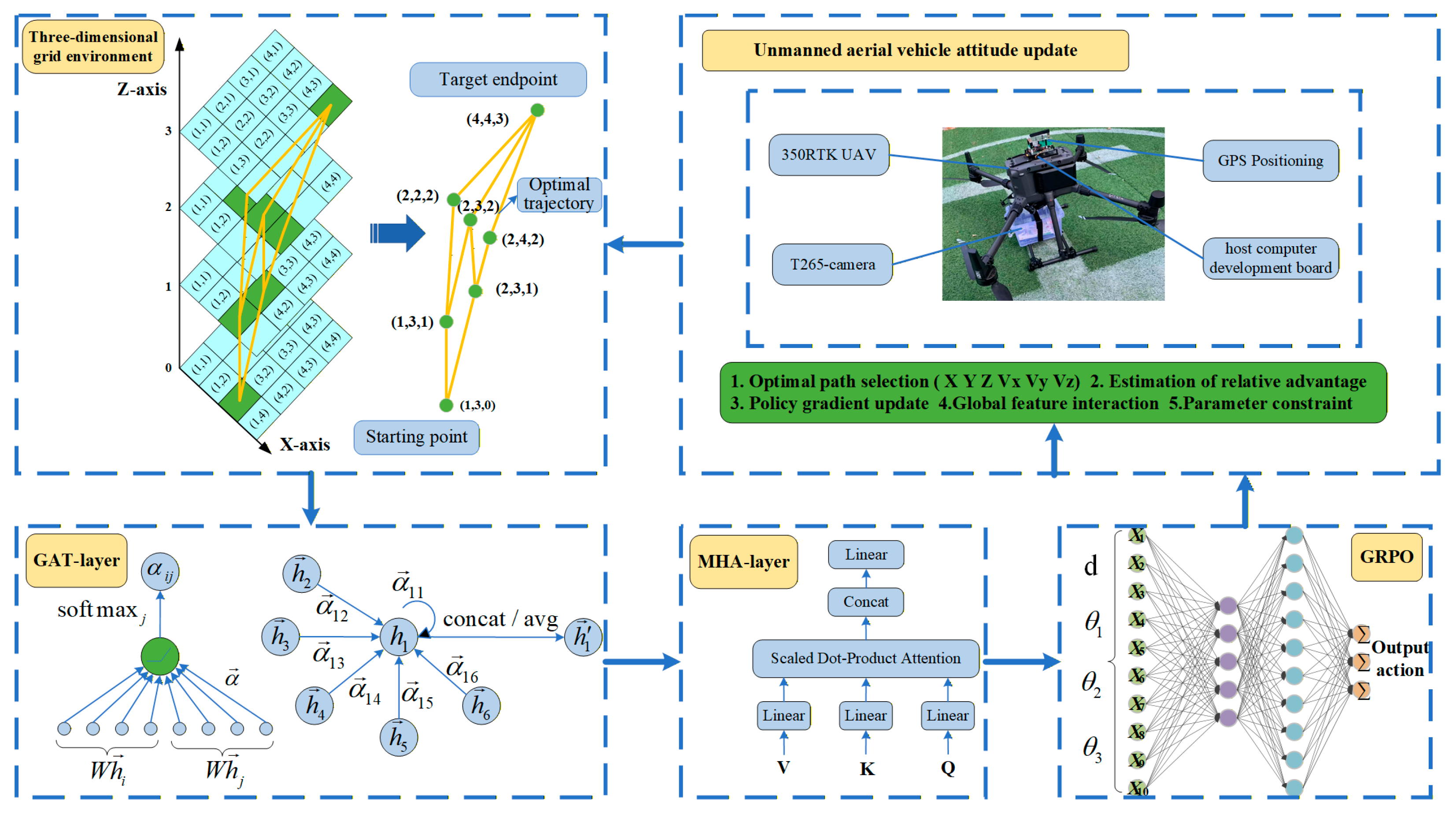
Figure 1. G-MAPONet fusion algorithm framework.
Drones 09 00871 g001
Figure 2. Flight altitude constraint diagram.
Drones 09 00871 g002
Figure 3. Experimental process of G-MAPONet fusion algorithm.
Drones 09 00871 g003
Figure 4. Two-dimensional raster environment trajectory planning: (a) Inter Path planning (2D); (b) Gat Path planning (2D); (c) Pos Path planning (2D); (d) Self Path planning (2D); (e) Mha Path planning (2D); (f) Gat_Mha Path planning (2D).
Drones 09 00871 g004
Figure 5. Three-dimensional raster environment trajectory planning: (a) Self Path planning (3D); (b) Inter Path planning (3D); (c) Pos Path planning (3D); (d) Gat Path planning (3D); (e) Mha Path planning (3D); (f) Gat_Mha Path planning (3D).
Drones 09 00871 g005aDrones 09 00871 g005b
Figure 6. UAV trajectory planning flight process: (a) Waypoint 1; (b) Waypoint 2; (c) Waypoint 3; (d) Waypoint 4; (e) Waypoint 5; (f) Landing completed.
Drones 09 00871 g006
Figure 7. Four Algorithms 3D Path Planning Comparison: (a) GRPO; (b) Gat_GRPO; (c) Mha_GRPO; (d) G-MAPONet.
Drones 09 00871 g007
Figure 8. Six Algorithms 3D Path Planning Comparison: (a) GRPO Algorithm; (b) PPO Algorithm; (c) TRPO Algorithm; (d) A3C Algorithm; (e) DQN Algorithm; (f) G-MAPONet Algorithm.
Drones 09 00871 g008aDrones 09 00871 g008b
Figure 9. Two-dimensional environment training results: (a) Success Rate comparison (2D); (b) Comparison of Loss Values (2D); (c) Average Reward comparison (2D); (d) Reward Distribution Comparison (2D).
Drones 09 00871 g009
Figure 10. Three-dimensional environment training results: (a) Success Rate Comparison (3D); (b) Comparison of Loss Values (3D); (c) Average Reward Comparison (3D); (d) Reward Violin Box Plot per Strategy (3D).
Drones 09 00871 g010
Figure 11. Two Algorithms 3D Path Planning Comparison Training result: (a) 4Alg Reward Comp Curves (100); (b) LC-Comp-4Alg (100); (c) 4Alg Reward CompCurves (100); (d) Reward Distribution of Algorithms (100); (e) 4Alg Reward Comp Curves(300); (f) LC-Comp-4Alg (300); (g) 4Alg Reward CompCurves (300); (h) Reward Distribution of Algorithms (300); (i) 4Alg Reward Comp Curves (500); (j) LC-Comp-4Alg (500); (k) 4Alg AvgReward CompCurves (500); (l) Reward Distribution of Algorithms (500).
Drones 09 00871 g011aDrones 09 00871 g011b
Figure 12. Six Algorithms 3D Path Planning Comparison Training result: (a) 6Alg Reward Comp Curves (100); (b) LC-Comp-6Alg (100); (c) 6Alg AvgReward CompCurves (100); (d) Reward Distribution of Algorithms (100); (e) 6Alg Reward Comp Curves (300); (f) LC-Comp-6Alg (300); (g) 6Alg AvgReward CompCurves (300); (h) Reward Distribution of Algorithms (300); (i) 6Alg Reward Comp Curves (500); (j) LC-Comp-6Alg (500); (k) 6Alg AvgReward CompCurves (500); (l) Reward Distribution of Algorithms (500).
Drones 09 00871 g012aDrones 09 00871 g012b
Figure 13. The results of GRPO and G-MAPONet algorithms: (a) NCE Performance Heatmap; (b) AR Performance Heatmap.
Drones 09 00871 g013
Figure 14. Results of Different Reinforcement Learning Algorithms: (a) NCE Comparison; (b) AR Comparison.
Drones 09 00871 g014
Figure 15. Three-dimensional Grid Environment Trajectory Planning: APF as Benchmark: (a) GRPO vs. APF Path (3D); (b) DQN vs. APF Path (3D); (c) A3C vs. APF Path (3D); (d) PPO vs. APF Path (3D); (e) TRPO vs. APF Path (3D); (f) G-MAPONet vs. APF Path (3D).
Drones 09 00871 g015aDrones 09 00871 g015b
Figure 16. Three-dimensional Grid En3D Grid Path Planning: Reward and Obstacle Avoidance Metrics: (a) Final Reward Value; (b) Obstacle Avoidance Success Rate.
Drones 09 00871 g016
Table 1. Data Analysis of the Ablation Study of the G-MAPONet Algorithm.
AlgorithmNENCEARPPTC
GRPO100121−3.6564×
30019413.7749
5001679.8589
Gat_GRPO100196.5567
3004218.2423
5003819.2321
Mha_GRPO1003713.5614
3003618.1224
5005419.7308
G-MAPONet1001219.2423
3001420.4214
5002320.6417
Table 2. Comparison of Different RL Algorithms.
AlgorithmNENCEARPPTC
GRPO100100−5.61×
3002086.98
500696.99
G-MAPONet100407.86
3002419.12
5001519.24
PPO100526.45×
3003115.39
5001718.77
TRPO100100−4.59×
300300−5.34×
500500−15.96×
A3C10063−0.06×
300531.66
500665.36
DQN100100−53.89
300150−124.89×
500354−271.69
Table 3. Different RL Algorithms Comparison: APF as Benchmark.
Attention MethodFRVOASR
GRPO105.84650.9508
G-MAPONet162.49490.9922
PPO148.92170.8536
TRPO109.48370.4700
A3C81.89080.0117
DQN112.58330.9427
APF149.54760.9824
Disclaimer/Publisher’s Note: The statements, opinions and data contained in all publications are solely those of the individual author(s) and contributor(s) and not of MDPI and/or the editor(s). MDPI and/or the editor(s) disclaim responsibility for any injury to people or property resulting from any ideas, methods, instructions or products referred to in the content.