Application of UAVs and Machine Learning Methods for Mapping and Assessing Salinity in Agricultural Fields in Southern Kazakhstan

Highlights

What are the main findings?

• A method for quickly assessing field salinity has been developed based on the use of a UAV equipped with a multispectral camera and laboratory studies of the electrical conductivity of soil samples.
• Labeled datasets have been developed for tuning machine learning models and mapping field salinity in southern Kazakhstan.

What is the implication of the main finding?

• The use of a UAV equipped with a multispectral camera and machine learning methods enables highly detailed salinity mapping of large field areas.
• Conditions in each field can vary; therefore, achieving expected results requires individual tuning of the models for each field.

Abstract

Soil salinization is an important negative factor that reduces the fertility of irrigated arable land. The fields in southern Kazakhstan are at high risk of salinization due to the dry arid climate. In some cases, even the top layer of soil has a significant degree of salinization. The use of a UAV equipped with a multispectral camera can help in the rapid and highly detailed mapping of salinity in cultivated arable land. This article describes the process of preparing the labeled data for assessing the salinity of the top layer of soil and the comparative results achieved due to using machine learning methods in two different districts. During an expedition to the fields of the Turkestan region of Kazakhstan, fields were surveyed using a multispectral camera mounted on a UAV; simultaneously, the soil samples were collected. The electrical conductivity of the soil samples was then measured in laboratory conditions, and a set of programs was developed to configure machine learning models and to map the obtained results subsequently. A comparative analysis of the results shows that local conditions have a significant impact on the quality of the models in different areas of the region, resulting in differences in the composition and significance of the model input parameters. For the fields of the Zhetisay district, the best result was achieved using the extreme gradient boosting regressor model (linear correlation coefficient Rp = 0.86, coefficient of determination R² = 0.42, mean absolute error MAE = 0.49, mean square error MSE = 0.63). For the fields in the Shardara district, the best results were achieved using the support vector machines model (Rp = 0.82, R² = 0.22, MAE = 0.41, MSE = 0.46). This article presents the results, discusses the limitations of the developed technology for operational salinity mapping, and outlines the tasks for future research.

1. Introduction

Anthropogenic factors, causing a sharp increase in the intensity of soil and water resource use, as well as climate change, lead to increased salinity and subsequent land degradation, especially in arid regions of Earth [1]. Currently, more than 20% of irrigated land is salinized to different degrees [2], and over the past 30 years, the area of such land has increased by 2.4 times [3]. There are numerous examples of negative changes that have led to an increase in the area of salinized land [4] and production problems, especially in arid regions. Such phenomena are characteristic of Central Asia as a whole [5], where there are large areas of land and limited water resources. The lands of southern Kazakhstan are an example of such negative changes. For example, in the Kyzylorda region, almost 85% (20.3 million hectares) of the total land area (22.6 million hectares) is salinized [6], and in the Turkestan region, 32% of cultivated fields are salinized [7]. In total, saline soils cover more than 40 million hectares in Kazakhstan [8]. In this regard, a number of strategic documents of the Government of Kazakhstan set out plans for the development of crop production [9] and modernization of agriculture [10], including through the use of digital technologies [11]. Overcoming negative factors and increasing crop production volumes is achieved through the development of precision farming technologies [12]. Precision farming involves managing agricultural production in both spatial and temporal terms, where cultivated fields and their plots are considered individually; moreover, only the necessary resources are used [13]. This approach allows minimization of the amount of agrotechnical operations and costs associated with chemical and biological (pesticides, herbicides, etc.) impacts on fields, while ensuring optimal conditions for the growth and development of crops. To implement these technologies, it is necessary to obtain accurate and timely information about the condition of fields and crops. The most common way to obtain this type of information is employment of satellite products based on Sentinel-1,2, Terra, Landsat, Kompsat, Modis, Aster, and other satellite images [14].

These capabilities are implemented in a number of agricultural monitoring systems: EODSA crop monitoring [15], Cropinno [16], Cropwise [17], and others. However, such systems have limitations related to the frequency of information updates, the influence of the atmosphere, low spatial resolution, and the significant cost of high-quality satellite images. The use of UAVs, equipped with multispectral cameras for the purpose of providing information for precision farming processes, has significant advantages:

• Multispectral cameras mounted on UAVs allow data acquisition on plant condition with a resolution of several millimeters, ensuring high accuracy of analysis [18].
• UAVs can quickly cover large areas that are inaccessible to ground surveys and provide real-time data, allowing rapid response to changes in the plant condition [19,20].
• UAVs can easily reach hard-to-reach areas, making them indispensable in difficult terrain [19].

These advantages are primarily reflected in the high-precision and rapid mapping of agricultural fields [21]. The obtained images and maps are employed for monitoring purposes [22,23] using a wide range of computational methods. One of these tasks, relevant for agricultural fields in Kazakhstan, is the assessment of soil salinity. Low and medium soil salinity leads to physiological drought in cultivated plants due to disruption of ion homeostasis. High salinity causes osmotic stress, in which water stops flowing to the roots of plants, leading to their death. Thus, for optimal cultivation of agricultural crops, it is necessary to identify areas of soil salinization in order to plan agrotechnical measures to combat salinization or make decisions about cultivating salt-tolerant crops. Ground surveys are traditionally used to solve such problems. However, due to their high labor intensity and cost, their use is very limited. Therefore, the use of remote sensing methods is relevant. With the appearance of publicly available satellite products for salinity mapping, radar [24,25,26], optical [27], hyper- [28] and multispectral [29] data and their combinations [30,31,32] are used. The multispectral channels of the obtained images and spectral indices serve as a source for identifying long-term trends [33] and are used as input data for machine learning models [34], which are successfully applied to study salinity at local [32,35], regional [30], and global scales [36]. However, as is noted above, the resolution of publicly available satellite products does not allow the identification of small-sized areas of salinity. Moreover, the acquisition of optical band data depends on weather conditions, and variations in environmental conditions, irrigation, and weather lead to changes that may not be reflected in satellite data. The fact still remains that salinity is difficult to identify quickly and varies over temporal and spatial scales. However, inexpensive multispectral data obtained with the use of unmanned aerial vehicles (UAVs) can be used to assess heterogeneous soil properties such as water content and electrical conductivity [37].

The number of scientific studies in this field has more than doubled between the end of 2020 and the beginning of 2023, which is a sign of a rapidly developing area of scientific research [38]. At the same time, the task of processing data obtained from UAVs is currently the most popular in the scientific community [39]. There are numerous examples of studies on the use of multi- and hyperspectral images obtained from UAVs and machine learning methods to assess soil salinity [35,40,41,42,43,44,45,46]. In these studies, the coefficient of determination in salinity assessment models ranges from 0.4 to 0.835.

Thus, the use of a low-altitude flying platform equipped with a multispectral or hyperspectral camera allows rapid multichannel mapping of agricultural fields to assess soil salinity [47,48,49]. However, the results of such analysis depend significantly on the local conditions, soil sampling conditions, humidity, vegetation cover, and the selected machine learning algorithms. Therefore, despite the promising results reported in the literature and obtained in our own research [41], the following tasks remain unresolved:

(1)

How much do weather conditions, lighting, soil type, and existing vegetation affect the results of assessing the salinity level of agricultural fields?

(2)

How much do the climatic and landscape conditions of the analyzed agricultural area affect the results?

(3)

What is the optimal configuration of UAV attachments?

(4)

What is the optimal amount of field data to ensure sufficient accuracy in determining salinity?

(5)

What are the optimal methods for preprocessing the collected data, and what combinations of input parameters and machine learning algorithms provide the most accurate and stable results?

In this article, the author attempts to answer questions (2), (3), (4), and (5) through a comparative analysis of salinity mapping results obtained in different fields. This paper considers the technological framework of UAVs, ground surveys, and machine learning methods for monitoring the salinity of agricultural fields in the Turkestan region of Kazakhstan.

The main contributions of the study are as follows:

• Development of a methodological scheme for obtaining the current salinity maps of fields in Southern Kazakhstan using multispectral imaging from a UAV, which allows high spatial and temporal resolution to be achieved and significantly reduces dependence on expensive ground-based soil surveys.
• Implementation of a comparative analysis using the high-detail surface soil salinity mapping technologies for two regions of southern Kazakhstan; this allows a more accurate identification of the limitations of the method under development.
• Development of a dataset, which allows configuration and investigation of the behavior of various machine learning models in the process of assessing salinity based on a combination of multispectral data from UAVs and soil conductivity estimates.

This paper consists of the following sections:

Section 2 briefly describes the area of the conducted field research.

Section 3 describes the methods and tools used to collect and process data.

Section 4 describes the results obtained.

Section 5 presents the discussion on the topic.

Section 6 describes the advantages and limitations of the method.

The conclusion summarizes the research and sets the tasks for further research.

2. Regions Under Research

Agricultural fields were surveyed in the Shardara and Zhetisay districts of the Turkestan region of Kazakhstan (see Figure 1), near one of the major rivers of Central Asia, the Syr Darya.

The districts under consideration have relatively close locations but differ in their geographic parameters. The Shardara district is located on the eastern edge of the Kyzylkum desert. The landscape is semi-desert and flat. Elevations range from 200 to 300 m above sea level. The climate is sharply continental and arid, with hot summers and mild winters. The soil is predominantly sandy and sandy loam, with low natural fertility. The main specialization is crop production (cotton, grain crops, melons) and livestock raising. The water source is the Shardara Reservoir and the Syr Darya River. Intensive irrigation is required for crop cultivation. Flight tests were conducted over an area of 52.75 hectares. The Zhetisay district is located further to the south, near the border of Uzbekistan. The relief is predominantly flat, with elevations of approximately 150–250 m. The climate is dry, with long, hot summers, requiring intensive irrigation. The district is one of Kazakhstan’s cotton-growing centers. Vegetables, melons, and grains are also grown. The soil is more fertile and predominantly gray. The district has a well-developed network of irrigation channels. The main water source is the Shardara Reservoir. Survey flights covered an area of 23.43 hectares. The regions belong to the irrigated zone of the arid lands of southern Kazakhstan where, due to high insolation and infrequent rainfall, cases of soil salinization are common, especially at the end of the growing season. The research methodology is described below in Section 3.

3. Materials and Methods

The research process consisted of the following stages (see Figure 2):

A.

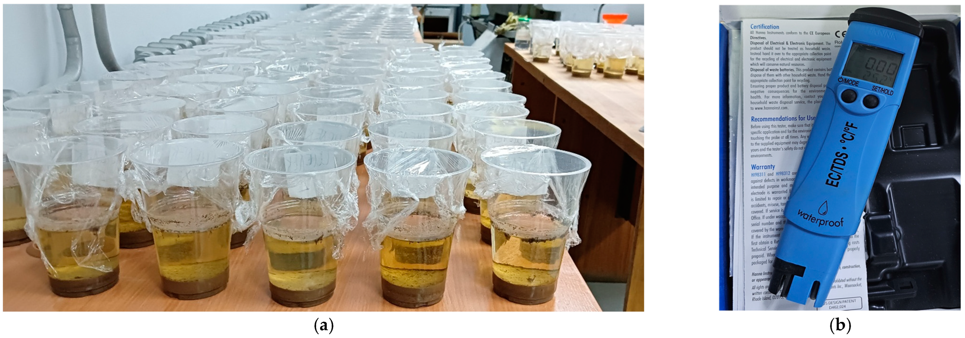
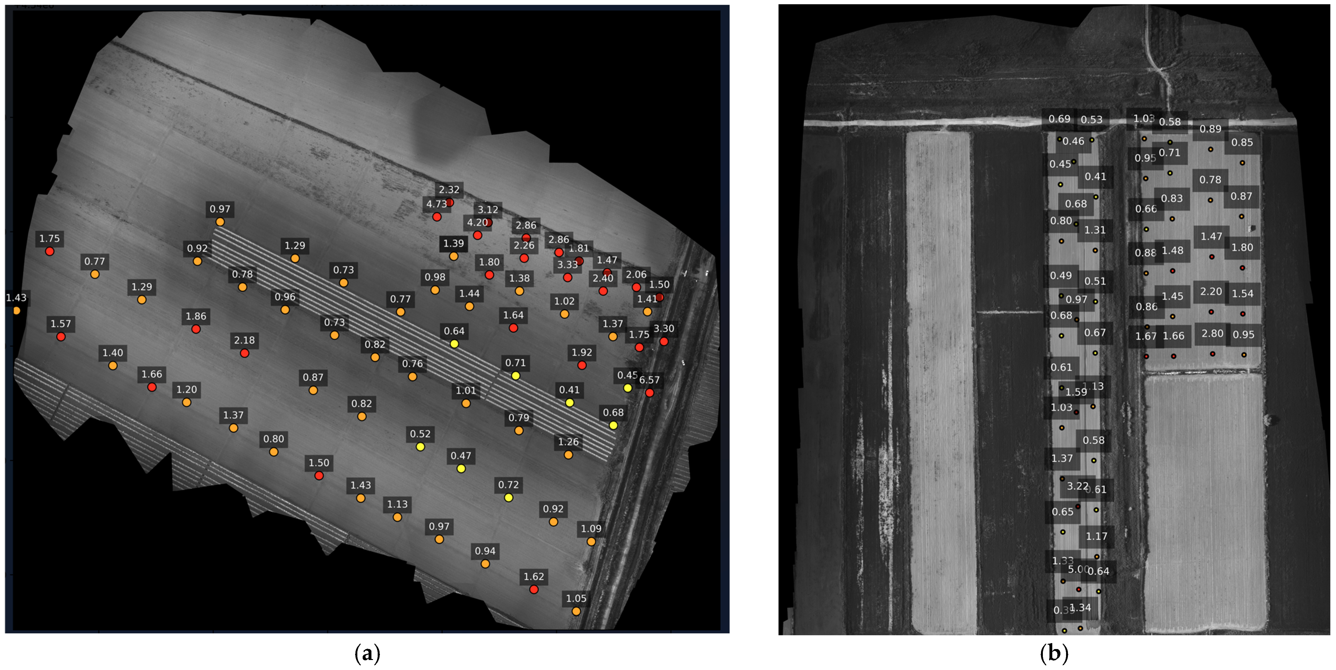
Ground samples were taken from the depth of 10–20 cm in the accessible part of the fields. The locations of the sampling points were recorded. The samples were processed in the laboratory to assess their electrical conductivity.

B.

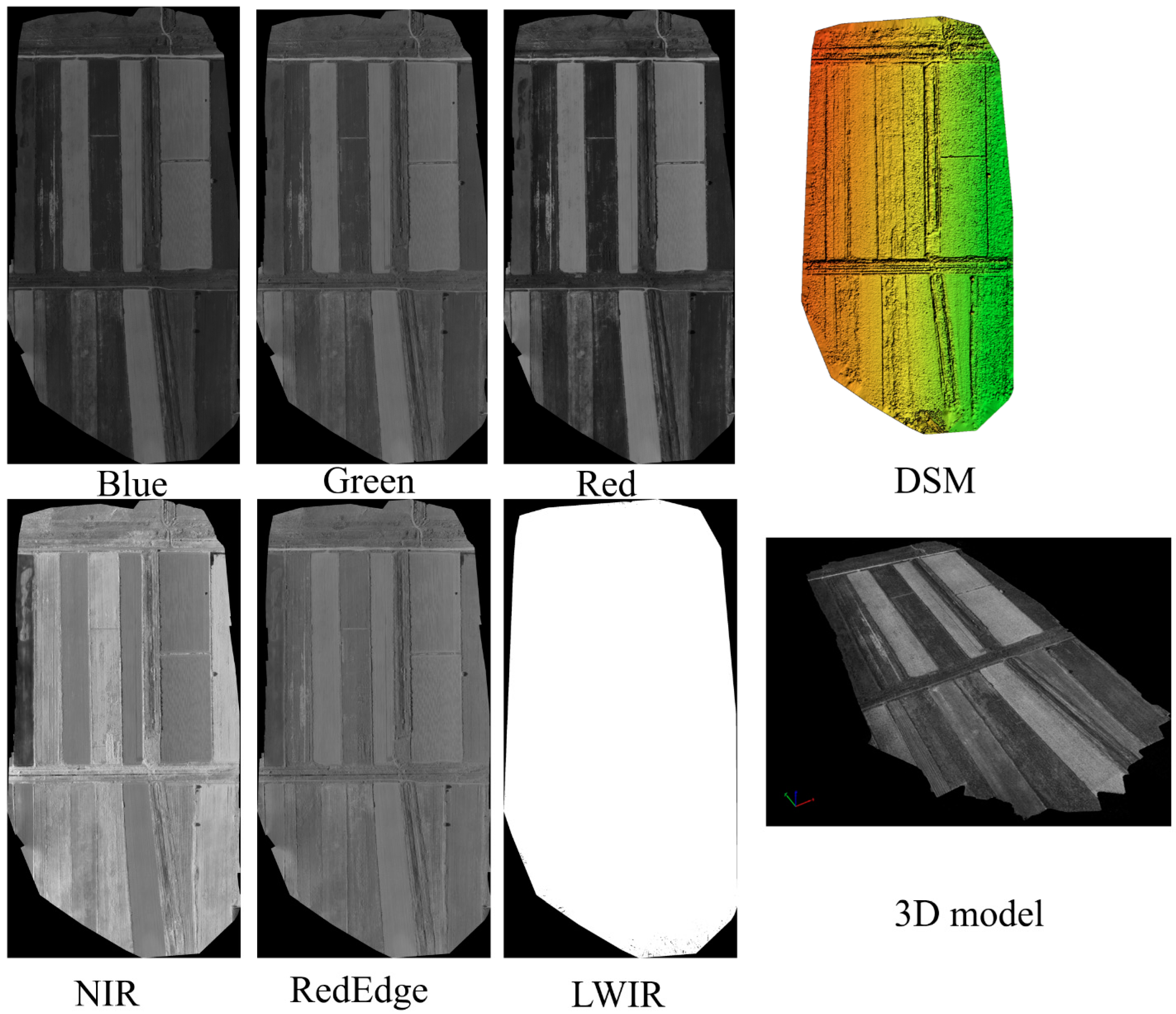
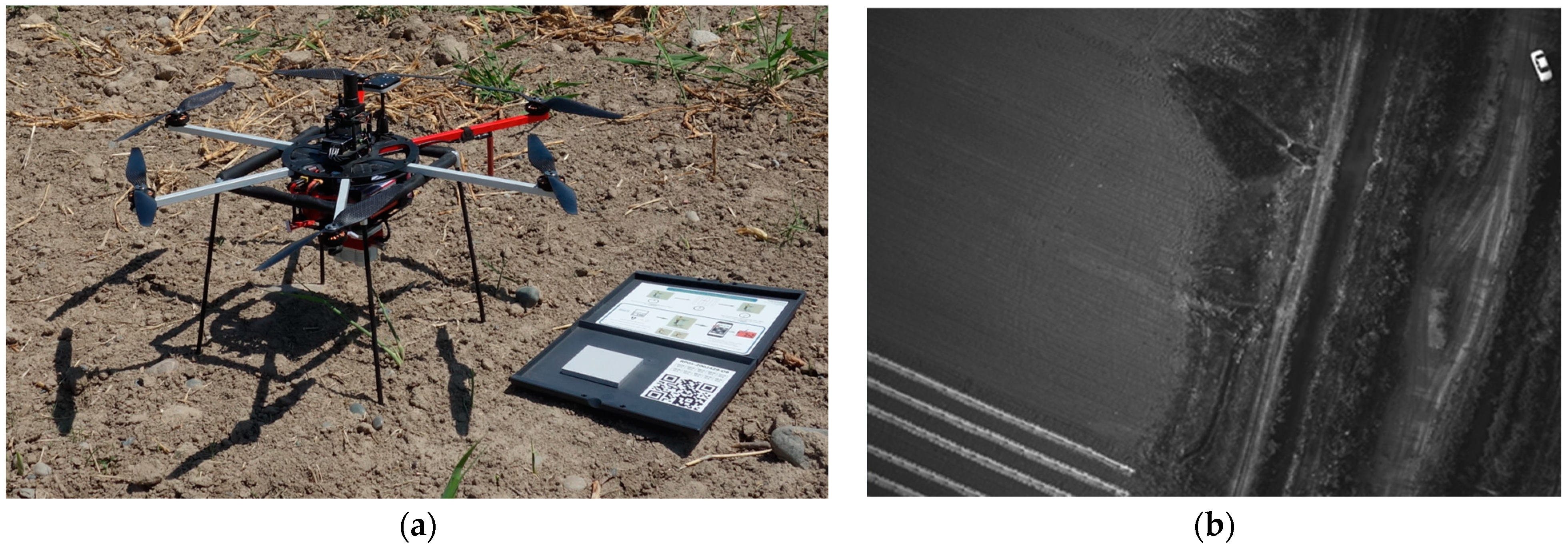
The fields were flown over, and multispectral images were obtained. The multispectral images were processed to obtain spectrum maps, spectral indices, and a DSM map.

C.

Using the obtained data, a set of input features was formed and a target variable (electrical conductivity) was determined.

D.

Machine learning models and spectrum map preprocessing parameters were configured, and the model with the best results was selected.

E.

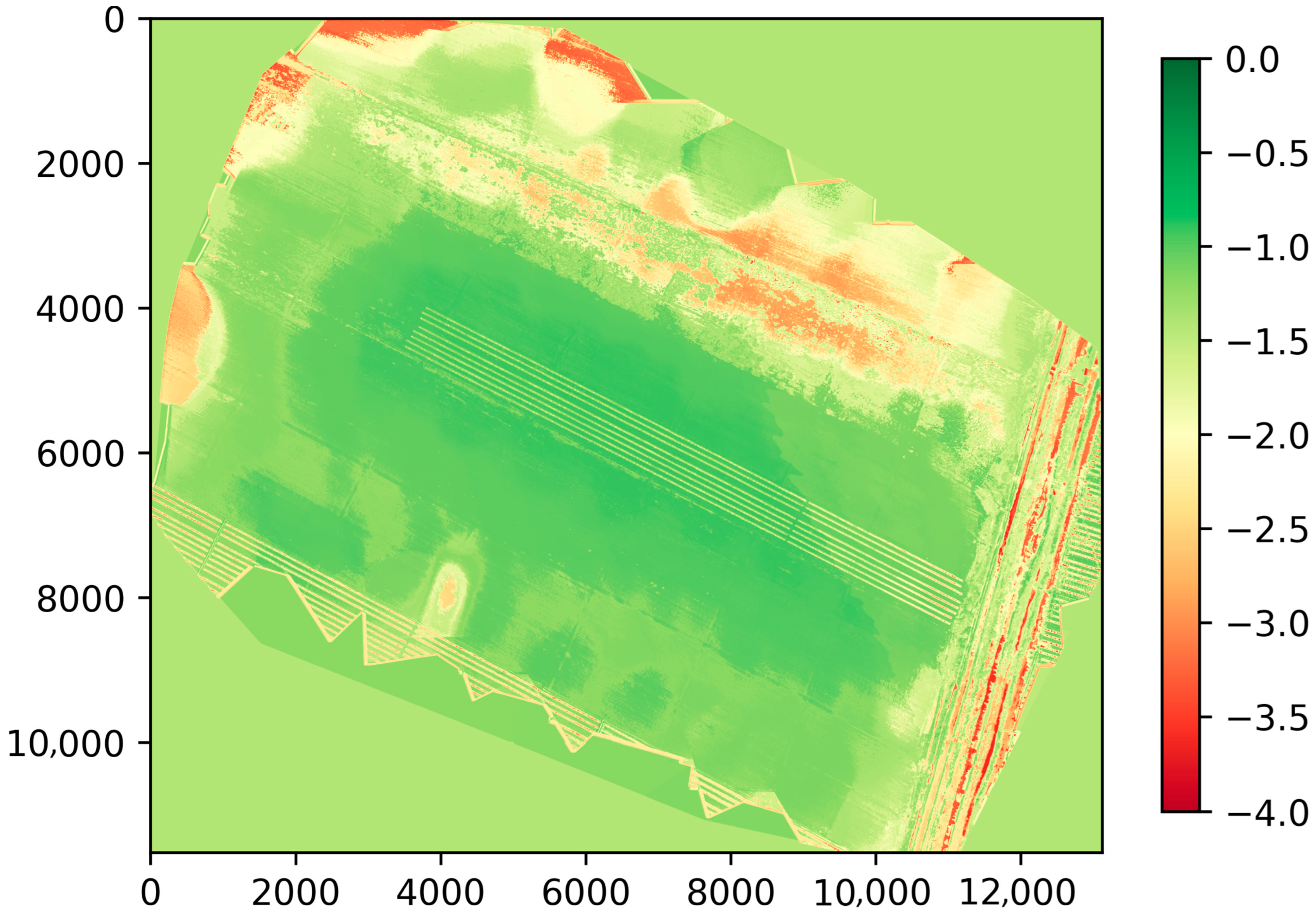
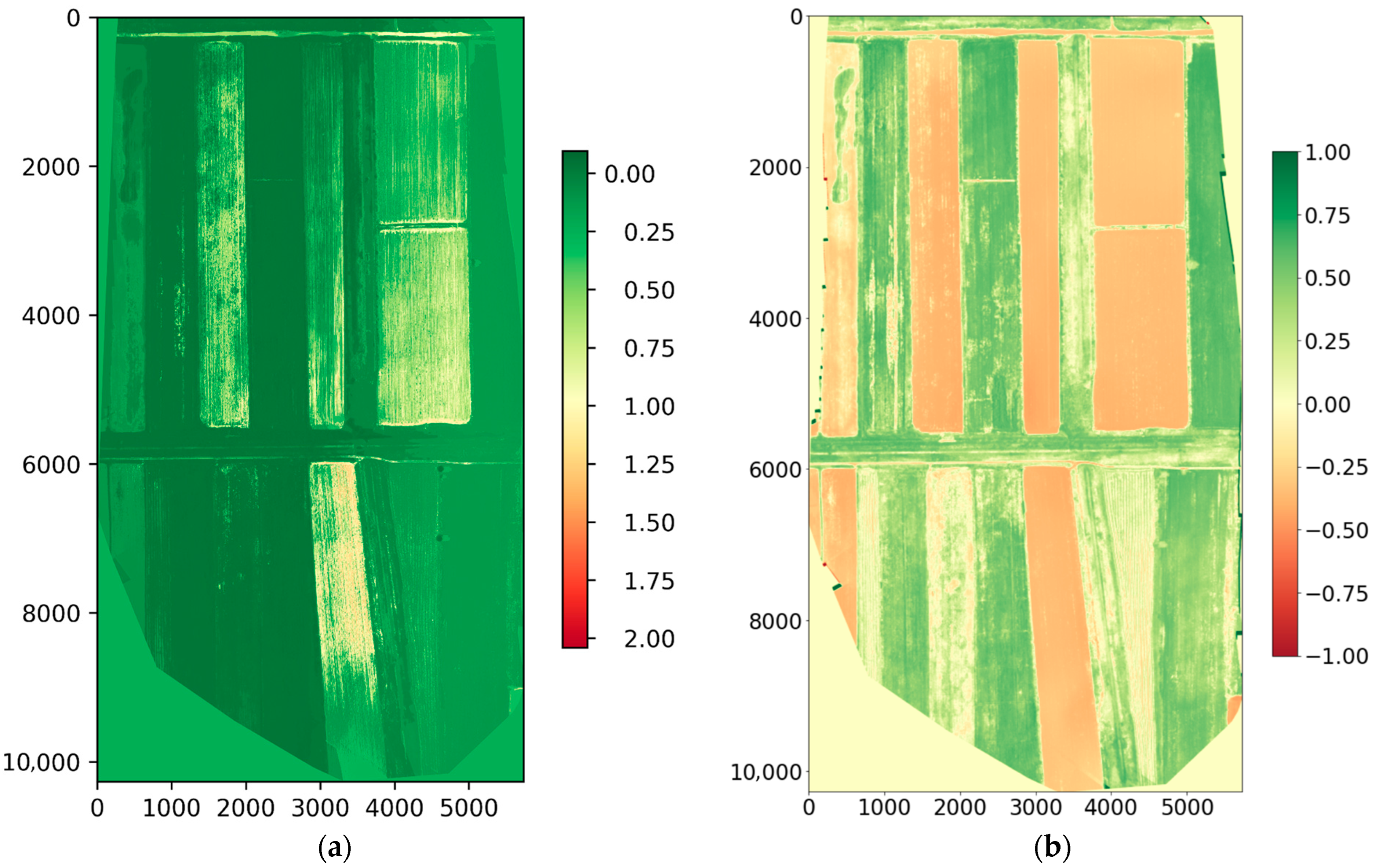
Using the machine learning model, the salinity maps of the fields at the time of data collection were obtained.

Further, we briefly review the research stages listed above.

The flights took place on 19 May 2023 and on 20 May 2023 in clear, sunny weather. The fields are located at an altitude of approximately 250 and 220 m above sea level in the Zhetisay and Shardara districts, respectively. As a result of the UAV flights, more than 5000 (3750 + 2112) multispectral images were obtained (camera: MicaSense Altum, aperture f/1.1, exposure 1/30 s). At the same time, soil samples were collected during the day and then delivered to the laboratory for testing. At the time of the expedition, plants were in the early stages of development in the field (see Figure 3 and Figure 4).

3.1. Field Survey

The field survey was performed using a specially designed unmanned aerial platform equipped with a Micasense Altum PT multispectral camera [50] (see Figure 3; source: generated by the author). The camera has the following spectral channels: blue (475 nm ± 32 nm), green (560 nm ± 27 nm), red (668 nm ± 14 nm), red edge (717 nm ± 12 nm), Near-IR (nir) (842 nm ± 57 nm), as well as a thermal channel (LWIR) with a resolution of 160 × 120 pixels. One of the images in the nir range, obtained from the camera during the flights, is shown in Figure 3b. The photographs obtained during the flights have an average overlap of 80%.

3.2. Soil Sampling and Electrical Conductivity Assessment

Soil samples were collected simultaneously with UAV field surveys. Soil samples were collected from a shallow depth (approximately 10–20 cm), with a distance of approximately 50 m between collection sites. Each sample was labeled and placed in a sealed bag. The coordinates of the collection sites were recorded using a Garmin 65 device with a positioning accuracy of about 5 m (see Figure 4a–c; source: generated by the author).

The soil samples were weighed and then dried for 5–9 days, without using special drying agents, at a room humidity of about 15%. After drying, vegetation residues, stones, and other solid insoluble objects were removed from each sample by sieving. In order to dissolve the salts contained in the soil, after sieving, the samples were mixed with water in a ratio of 1:5 (1 part of soil by weight to 5 parts of water), as is usually performed in tasks involving the measurement of the electrical conductivity of soil solutions [26,38]. The resulting solutions were left to stand for 24 h to allow the salts to dissolve completely and the solid particles to settle (see Figure 5a). The electrical conductivity of the solution was then measured using a Hanna EC/TDS tester DIST 5&6 (see Figure 5b; source: generated by the author).

The locations of soil sampling points were mapped using Python 3.6 and the rasterio library, designed for reading and writing several different raster formats in Python (TIFF, GeoTIFF, ASCII Grid, etc.) [51]. The locations of the sampling points and the obtained electrical conductivity values are shown in Figure 6a,b. Source: generated by the author. The colors of the markers are described in

Table 1. Soil salinity classes based on electrical conductivity (EC1:5 and ECe).

Salinity Class	EC1:5 for Sands (dS/m)	EC1:5 for Loams (dS/m)	EC1:5 for Clays (dS/m)	ECe (dS/m)	Color on Map	Color of Marker
Unsalted	0–0.14	0–0.18	0–0.25	0–2	Green
Lightly salted	0.15–0.28	0.19–0.36	0.26–0.50	2–4	Blue
Moderately salted	0.29–0.57	0.37–0.72	0.51–1.00	4–8	Yellow
Heavily salted	0.58–1.14	0.73–1.45	1.01–2.00	8–16	Orange
Very heavily salted	1.15–2.28	1.46–2.90	2.01–4.00	16–32	Red
Extremely salted	>2.28	>2.90	>4.00	>32	Red

.

The electrical conductivity of the solution determined six or fewer salinity classes in accordance with Table 1 [52].

3.3. Multispectral Images Processing

Images processing was implemented with employment of PIX4D version 4.5.6 [53] with the set Standard 3D Map parameter. Image coordinate system: WGS 84 (EGM 96 Geoid); output coordinate system: WGS 84/UTM zone 42N (EGM 96 Geoid).

Image processing consisted of the following stages:

• Initial processing;
• Generation of orthophoto plan, multispectral maps, digital surface model (DSM), and digital terrain model (DTM);
• Calculation of spectral indices.

To calculate the salinity level of cultivated soil using machine learning methods, a wide range of spectral indices was calculated, including special spectral indices natural for various types of saline surfaces (see

Table 2. Spectral indices used in the machine learning model tuning process.

Spectral Indices	Ref.
$NDSI={\displaystyle \frac{red-nir}{red+nir}}$	[41]
$S1={\displaystyle \frac{blue}{red}}$	[42]
$S2={\displaystyle \frac{blue-red}{blue+red}}$	[42]
$S3={\displaystyle \frac{green\ast red}{blue}}$	[42]
$SI1=\sqrt[2]{green\ast red}$	[45]
$SI2=\sqrt[2]{gree{n}^2+re{d}^2+ni{r}^2}$	[44]
$SI3=\sqrt[2]{gree{n}^2+ni{r}^2}$	[35]
$SI8={\displaystyle \frac{blue\ast red}{green}}$	[45]
$WI1=0.1761\ast green+0.322\ast red+0.3396\ast nir$	[46]
$SSRI={\displaystyle \frac{nir}{\sqrt[2]{green\ast red}}}$	[48]
$NDSIre={\displaystyle \frac{red-red\_edge}{red+red\_edge}}$	[41]
$SI3re=\sqrt[2]{gree{n}^2+red\_edg{e}^2}$	[41]
$SSRIre={\displaystyle \frac{red\_edge}{\sqrt[2]{green\ast red}}}$	[41]
$WDVI=nir-0.1\ast red$	[54]
$NDWI={\displaystyle \frac{green-nir}{green+nir}}$	[55]
$DVI=nir-red$	[56]
$EVI=2.5\ast {\displaystyle \frac{nir-red}{(nir+6\ast red-7.5\ast blue+1)}}$	[57]
$GI={\displaystyle \frac{green}{red}}$	[58]

).

3.4. Customization of Machine Learning Models

The following machine learning models were used in this study (see

Table 3. List of machine learning models used in the research process. Source: generated by the author.

Abbreviated Name	Classifier	References
XGB	Extreme gradient boosting	[59]
GBT	Gradient boosted trees	[60]
kNN	k-Nearest neighbors	[61]
RF	Random forest	[62]
LR	Linear regression	[63]
MLP or ANN	Artificial neural network or multilayer perceptron	[64,65]
Lasso	Lasso Regression	[66]
ElasticNet	Elastic net	[67]
LGBM	Light gradient boosting machine	[68,69,70]
Ridge	Ridge regression	[71]
SVM	Support vector machines	[72]

).

The formulated task of assessing soil salinity is a regression task. To evaluate the quality of regression models, the metrics shown in

Table 4. Metrics for evaluating regression models. Source: generated by the author.

Metrics	Formula	Explanation
Mean absolute error	$MAE={\displaystyle \frac{{{\displaystyle \sum }}_{i=1}^n|y^{\left(i\right)}-h^{\left(i\right)}|}{n}}$	where n is the sample size; $y^{\left(i\right)}$ is the real value of the target variable for the i-th example; and $h^{\left(i\right)}$ is calculated value of the i-th example
Mean square error	$MSE={\displaystyle \frac{{{\displaystyle \sum }}_{i=1}^n{(y^{\left(i\right)}-h^{\left(i\right)})}^2}{n}}$
Determination coefficient	$R^2=1-{\displaystyle \frac{S{S}_{res}}{S{S}_{tot}}}$ $S{S}_{res}={\displaystyle {\displaystyle \sum }_{i=1}^n}{(y^{\left(i\right)}-h^{\left(i\right)})}^2$ $S{S}_{tot}={\displaystyle {\displaystyle \sum }_{i=1}^n}{(y^{\left(i\right)}-\overline{y})}^2,\overline{y}={\displaystyle \frac{1}{n}}{\displaystyle {\displaystyle \sum }_{i=1}^n}{y}^{\left(i\right)}$
Linear correlation coefficient (or Pearson correlation coefficient)	$Rp\left(y,h\right)={\displaystyle \frac{{{\displaystyle \sum }}_{i=1}^n(h_i-\overline{h})\left(y_i-\overline{y}\right)}{{{\displaystyle \sum }}_{i=1}^n{\left(y_i-\overline{y}\right)}^2{{\displaystyle \sum }}_{i=1}^n{(h_i-\overline{h})}^2}}$	where $\overline{h}={\displaystyle \frac{1}{n}}{{\displaystyle \sum }}_{i=1}^n{h}_i$

are commonly used [73]:

The process of preprocessing the spectral maps and tuning machine learning models included the following steps.

a.

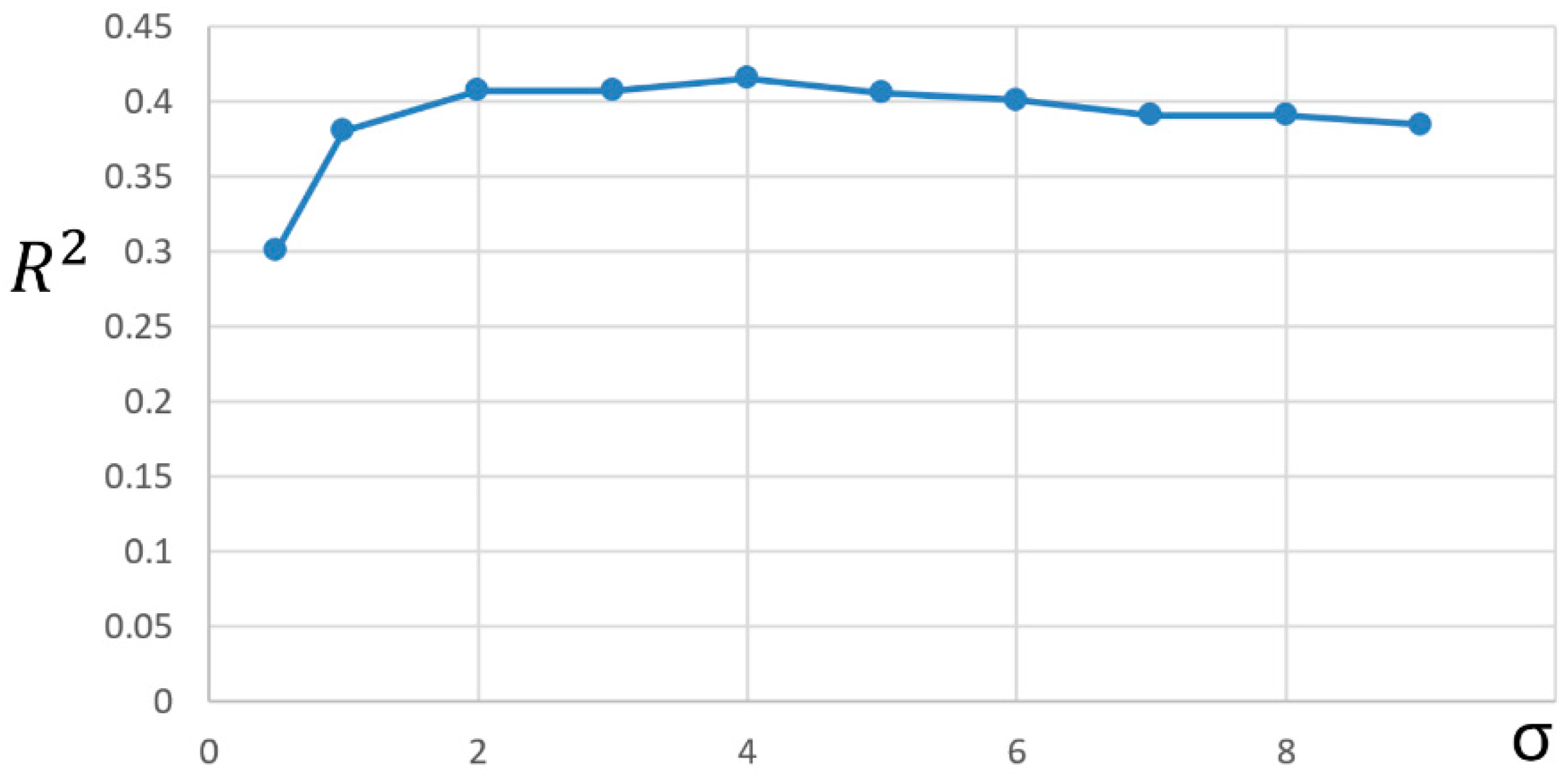
High-resolution images from UAVs can lead to large differences in images of small field fragments with similar salinity values due to the chaotic arrangement of clumps of soil. To level out these differences, images were smoothed using a Gaussian filter.

$$\mathit{G}\left(\mathit{x}\mathbf{,}\mathit{y}\right)={\displaystyle \frac{\mathbf{1}}{{\mathbf{2}\mathsf{\pi }\mathsf{\sigma }}^{\mathbf{2}}}}{\mathit{e}}^{-{\displaystyle \frac{{\mathit{x}}^{\mathbf{2}}+{\mathit{y}}^{\mathbf{2}}}{\mathbf{2}{\mathsf{\sigma }}^{\mathbf{2}}}}}$$

where σ is the standard deviation of the distribution, and x, y are coordinates.

The standard deviation parameter (σ) was selected by conducting a series of computational experiments using the scipy.ndimage library.

b.

The spectral channel values of the field images are extracted based on the coordinates of the collection points. Then, the spectral indices are calculated (see Table 2) and the resulting set of input parameters is fed into machine learning models (the model Table). During the experiments and visualization of the results, a significant systematic inaccuracy in the measurement of soil sample coordinates was discovered. The locations of the samples were additionally verified manually.

c.

The performance of machine learning models depends on input features. If there is an excessive set of parameters, the quality of the model’s performance may deteriorate significantly. The mlxtend library [74] was used to select significant features. The library allows the discarding of those input parameters that impair the predictive capabilities of the model.

d.

Given that the amount of data for training and validating models is small, cross-validation was used for their objective evaluation. In this study, the author used a cross-validation of random permutations—ShuffleSplit. In this case, the initial data is divided into training and test data in a given proportion (in our case, 80% are training data and 20% are test data). To ensure a statistically stable result, this division was performed 200 times for each regression model. The obtained model estimates (MAE, R², Rp) were averaged and taken as an assessment of the quality of each model.

A tuned machine learning model makes it possible to assess the influence of individual input parameters on the conclusions made by the algorithm. Agnostic explanation models, such as Shap [75], are very useful tools for this purpose. They are widely used to transform ‘black box’ models into ‘white’ or ‘gray’ boxes; in other words, models whose conclusions can be explained [76] (explainable machine learning models [77]). The main calculations were performed on a computer with the following specifications: CPU Intel(R) Core(TM) i7-10750H 2.60GHz, RAM 64GB, GPU1 Intel(R) UHD Graphics, GPU2 NVIDIA Quadro T2000.

4. Results

The technical results of the initial processing of images for the fields in the Shardara and Zhetisay districts are presented in Appendix C. Figure 7 shows the images of spectral channels, DSM maps, and a 3D model generated from photographs taken during flights over fields in the Zhetysay district. Similar spectral maps for the fields in the Shardara district are provided in Appendix B.

The obtained mapped data served as a source of actual values for the spectra and field terrains, which are compared with the electrical conductivity values during the machine learning model tuning process. Partial results of electrical conductivity measurements of soil sample solutions are presented in

Table 5. Results of electrical conductivity measurements of soil sample solutions. Source: generated by the author.

№	Longitude	Latitude	Altitude	Wet Sample Weight	Dry Sample Weight	Moisture Content	Conductivity
14	68.051052	41.92827	223.42334	187.61	178.3	5.22%	1.03
15	68.051074	41.927914	222.164368	244.42	228.95	6.76%	0.95
16	68.051088	41.927458	223.933487	177.25	172.94	2.49%	0.66
17	68.05109	41.927064	220.892654	168.5	163.87	2.83%	0.88
18	68.051109	41.926581	224.125793	181.6	175.55	3.45%	0.86
19	68.051105	41.926316	217.128967	213.16	203.73	4.63%	1.67
20	68.051432	41.926322	211.334152	257.06	243.25	5.68%	1.66
…	…	…	…	…	…	…	…
53	68.050303	41.924963	223.266144	172.81	163.85	5.47%	3.22

. The weight of the samples before drying (‘Wet sample weight’) and after drying (‘Dry sample weight’), the percentage of water evaporated after drying (‘Moisture content’), and the electrical conductivity of the solution are recorded. The table shows that sample number 14 is moderately salty, samples numbers 14, 15, 17, and 18 are very salty, samples 19 and 20 are extremely salty, and sample 53 is exceptionally salty.

For each district, a separate dataset was created, including spectral index values and conductivity measurements at the sampling points. The dataset for the Shardara district contains 53 values, while the dataset for the Zhetisay district contains 76 conductivity values. Conductivity values were used as the target variable when setting up regression models, and sampling point coordinates (longitude and latitude) were used to obtain spectral channel values and the following calculation of spectral indices. Machine learning models were tuned separately on each dataset. Thus, based on the actual conductivity data of soil samples, models were developed that can predict conductivity using spectral index values and DSM. To evaluate model performance, we applied the ShuffleSplit method along with standard regression quality metrics described in Table 4. The primary metric is the coefficient of determination.

During the first stage of adjusting the salinity prediction models, a systematic error in calculating the coordinates for the fields in the Shardara district, which amounted to 12 m in longitude, was eliminated. Then, experiments on finding the optimal set of input parameters for machine learning models were conducted, and the hyperparameters of the models were selected. Mlxtend was used to specify the set of features; it improved the predictive capabilities of the model by approximately 2 times. The best set of features for the fields of the Zhetisay district includes the following indicators: ‘DSM’, ‘NDWI’, ‘DVI’, ‘EVI’, ‘GI’, ‘NDSI’, ‘S1’, ‘S2’, and ‘SSRIre’. Similarly, for the fields of the Shardara district, the following set is the best one: ‘DSM’, ‘EVI’, ‘GI’, ‘SI3’, ‘SI8’, ‘WI1’, ‘nir’, and ‘red_edge’. The values of the machine learning model hyperparameters, selected empirically, are presented in

Table 6. Hyperparameters of regression models. Source: generated by the author.

Regression Model	Params
XGB	XGBRegressor(base_score=0.5, booster=‘gbtree’, colsample_bylevel=0.5,        colsample_bynode=1, colsample_bytree=0.7, early_stopping_rounds=50,        eval_metric=‘rmse’, gamma=0.0, gpu_id=−1, importance_type=‘gain’,        interaction_constraints=‘’, learning_rate=0.02, max_delta_step=0,        max_depth=2, min_child_weight=1, missing=nan,        monotone_constraints=‘()’, n_estimators=100, n_jobs=−1, nthread=8,        num_parallel_tree=1, random_state=0, reg_alpha=0, reg_lambda=1,        scale_pos_weight=1, subsample=0.8, tree_method=‘exact’,        validate_parameters=1, verbosity=None)
GBT	GradientBoostingRegressor(random_state=42)
kNN	KNeighborsRegressor()
RF	RandomForestRegressor(max_depth=6)
LR	LinearRegression()
MLP	MLPRegressor(hidden_layer_sizes=(10, 30), max_iter=250, random_state=42)
Lasso	Lasso(alpha=0.01)
ElasticNet	ElasticNet(alpha=0.02)
LGBM	{‘boosting_type’: ‘gbdt’, ‘objective’: ‘regression’, ‘metric’: {‘l1’, ‘l2’}, ‘num_leaves’: 2, ‘learning_rate’: 0.1, ‘feature_fraction’: 0.9, ‘bagging_fraction’: 0.8, ‘bagging_freq’: 5, ‘verbose’: 0, ‘max_depth’: 4, ‘num_iterations’: 100}
Ridge	Pipeline(steps=[(‘polynomialfeatures’,PolynomialFeatures(degree=3)), (‘ridge’, Ridge(alpha=35.5))])
SVM	SVR(C=0.695, gamma=2.7)

.

The parameters of the Gaussian filter (dispersion) were selected during computational experiments using the XGB regressor model, which demonstrated the best results (see Figure 8).

The optimal value of the standard deviation is σ = 4 for both regions. As a result, the following estimates of machine learning models were obtained (see

Table 7. Results of regression models for fields in the Zhetisay region. Source: generated by the author.

Duration (s)	Model	mMAE	mMSE	$\mathbf{m}{\mathbf{R}}^2$	$\mathbf{m}\mathbf{R}\mathbf{p}$
9.11652	XGB	0.4962	0.6277	0.4158	0.8623
7.312303	GBT	0.5307	0.6525	0.3087	0.8611
1.203192	kNN	0.5726	0.8689	0.2017	0.7782
28.34155	RF	0.5046	0.6052	0.4101	0.8638
0.492644	LR	4.5207	1850.976	−3024.31	0.7335
26.82196	MLP	0.595	0.8605	0.2047	0.7918
0.416424	Lasso	0.6054	0.8154	0.1924	0.8019
0.38149	ElasticNet	0.5891	0.8155	0.2164	0.8014
6.164825	LGBM	0.5777	0.8176	0.2126	NaN
0.692634	Ridge	0.5535	0.7601	0.2964	0.8316
0.457154	SVM	0.5064	0.7164	0.3564	0.8409

Notes. (1) mMAE, mMSE, $m{R}^2$, and $mRp$ are average values for 200 iterations of MAE, MSE, $R^2$, and $Rp$, respectively. (2) The best result is highlighted in bold.

).

The results of applying machine learning models to fields in the Shardara district are presented in Appendix A.

5. Discussion

The regression models employed in this study encompass several distinct classes: models based on decision tree algorithms (XGB, GBT, RF, LGBM); linear regression models (LR, Lasso, Ridge, ElasticNet); k-nearest neighbors; the simplest version of a multilayer neural network (MLP); and a support vector machine (SVM). Linear regression models and kNN have low flexibility. These models are stable: small changes in training data do not significantly affect predictions. They tend to underfit if the problem is complex. As a result, their performance in salinity estimation tasks is significantly inferior compared to the more complex models. From a practical standpoint, the choice between other models (XGB, GBT, RF, LGBM, SVM) is determined by ease of use and hyperparameter tuning.

Calculations also show that the best results are demonstrated by different machine learning models depending on the dataset. For the Zhetisay district, XGB demonstrates the best results, while for the Shardara district, SVM demonstrates the best results. The qualitative indicators of the models also differ significantly. Checking the significance of features using the Shap library showed the following results for the Zhetysai (see Figure 9a) and Shardara (see Figure 9b) districts.

Both similarities in the set of significant features and substantial differences can be observed. For example, the significance of DSM and EVI is quite high in both models. However, the spectral channels red_edge and nir are not used separately in models trained on data from the Zhetisay district (they are used as part of spectral indices), whereas in the Shardara district model they take a leading role.

This allows us to make a preliminary conclusion that local differences and field characteristics require separately configurating models for each study area. In both cases, terrain relief has a significant influence. The higher the area under consideration is relative to others, the lower its salinity is. Looking at the model quality metrics (see Table 7), it is possible to say that the predictive capabilities of the models are relatively limited. The conditions of data collection and the errors in resulting coordinate calculation introduce inaccuracies. In this sense, both models are significantly inferior to the previously developed model [41] and are satisfactory in accordance with [78], which states that a model is good if (R² ≥ 0.80), satisfactory (0.36 ≤ R² < 0.80), or not satisfactory (R² < 0.36).

The developed models were used to generate salinity maps of fields (see Figure 10 and Figure 11a).

The obtained maps show that surface salinity in the Zhetisay district during the period under review (20 May 2023) is significantly higher than in the Shardara district. It is most probable that the location of the Zhetisay district, surrounded on two sides by reservoirs, contributes to greater soil salinity. It should be noted that at the time of filming, the fields in the Shardara district had both plowed (almost vegetation-free) and overgrown areas. Since data collection was carried out only for plowed areas of the fields, the interpretation of the results should be based on the NDVI index values; in other words, we should take into account only the areas colored in orange in Figure 11b (areas with low NDVI values).

As is noted above, the salinity prediction models demonstrate low predictive power for the areas under consideration compared to the results reported in [45,79,80]. In author’s opinion, the reasons for this are as follows:

• Small amount of field data. For example, for the fields in the Shardara district, there are fewer than 50 measurements.
• Coordinate calculation errors. A systematic error in coordinate calculation, which arose for an unknown reason, led to unsatisfactory results at the initial stage. Manual correction improved the results but may not have been sufficient.
• Soil samples and surveys were performed using different positioning devices, each of which may introduce its own error.
• Soil sampling methodology. Unlike previous works, the soil samples were collected from a larger area of the fields, and the distance between samples was significantly greater.

Based on the results obtained, the following can be assumed:

• For these fields, it would be useful to conduct surveys at the time of intensive growth of useful plants in order to use plants as another indicator of salinity.
• Increasing the frequency of sampling will be useful for improving the quality of models.
• The use of visual landmarks and Real Time Kinematic systems [81] will significantly improve positioning accuracy.

6. Advantages and Limitations

The capabilities of the developed system depend equally on the equipment used and the data processing methods.

Mapping the agricultural fields using unmanned aerial vehicles (UAVs) equipped with multispectral cameras has its advantages and limitations.

Advantages are as follows (see [23,39]):

• High accuracy: UAVs are able to obtain data with high resolution and accuracy.
• Cost-effectiveness: The use of UAVs reduces costs compared to traditional aerial photography methods.
• Flexibility: UAVs can be used in areas that are difficult to access and dangerous for humans.
• Speed: Data collection and processing take less time compared to traditional methods.

Limitations are as follows [82]:

• High costs of equipment: Purchasing and maintaining drones and multispectral cameras can be expensive for small farms.
• Special skills required: Operating drones and analyzing data requires special training and skills.
• Weather restrictions: Drones may be limited in their use in adverse weather conditions, such as strong winds or rain.
• Legal and regulatory restrictions: Some regions have strict rules and restrictions on the use of drones, which can create some difficulties in using them.

Machine learning methods enable the mapping of surface soil salinity of large fields using relatively small amounts of field data. In essence, by collecting soil samples from a small portion of a field and tuning an appropriate predictive model, it becomes possible to estimate salinity levels for the entire field or even for adjacent fields within the same region. Despite the positive results, potential limitations of the proposed method for assessing surface soil salinity should be noted.

Overall limitations of the proposed method are as follows:

• The results are applicable at a specific time, since irrigation and other agronomic processes can significantly alter the distribution of salinity in the surface soil layer.
• Optical methods are unable to detect salinity in deep soil layers.
• The method does not include possible preprocessing of distorted images caused by shooting conditions. Such preprocessing (dehazing, deblurring, or illumination correction as described in [83,84]) can improve the result.
• Collecting and analyzing soil samples is a fairly labor-intensive process.
• Machine learning models require individual configuration for each group of fields.

7. Conclusions

Despite its shortcomings, the use of UAVs allows performing highly detailed imaging of the underlying surface. The obtained images serve as the basis for high-precision mapping and crop condition assessment using a wide range of specialized software tools. The DSM maps and index maps created allow the estimation of the health of vegetation, which in turn helps to plan and carry out agrotechnical measures to improve soil condition or cultivate useful plants.

As part of the current study, soil samples were collected along with field mapping. The obtained soil samples were examined in laboratory conditions with the purpose of determining their electrical conductivity. Using machine learning methods, the author performed a comparative assessment of the salinity of agricultural fields in the southern regions of Kazakhstan, which are irrigated by the Syr Darya River. Computational experiments allowed selection of the most accurate machine learning models: XGB for the Zhetisay region and SVM for the Shardara region. During the period under review, the salinity of the fields in the Zhetisay region was significantly higher compared to the average state.

The developed methodological scheme will be further applied for comparative evaluation of the method based on data obtained in other regions of Southern Kazakhstan. In future studies, the author plans to increase the number of soil samples, improve positioning accuracy, synchronize coordinate acquisition during sample collection with coordinates obtained from UAVs, add an image preprocessing module, and explore the possibility of applying deep learning models for mapping soil surface salinity.

References

- Li, X.; Wang, Z.; Song, K.; Zhang, B.; Liu, D.; Guo, Z. Assessment for Salinized Wasteland Expansion and Land Use Change Using GIS and Remote Sensing in the West Part of Northeast China. Environ. Monit. Assess. 2007, 131, 421–437. [Google Scholar] [CrossRef]
- Hossain, S. Present Scenario of Global Salt Affected Soils, Its Management and Importance of Salinity Research. Int. Res. J. Biol. Sci. 2019, 1, 1–3. [Google Scholar]
- Qadir, M.; Quillérou, E.; Nangia, V.; Murtaza, G.; Singh, M.; Thomas, R.J.; Drechsel, P.; Noble, A.D. Economics of Salt-Induced Land Degradation and Restoration. Nat. Resour. Forum 2014, 38, 282–295. [Google Scholar] [CrossRef]
- Chen, Y.; Zhang, W.-Y.; Wang, M.; Zhang, J.-H.; Chen, M.-X.; Zhu, F.-Y.; Song, T. Integrated Approaches for Managing Soil Salinization: Detection, Mitigation, and Sustainability. Plant Physiol. Biochem. 2025, 229, 110484. [Google Scholar] [CrossRef] [PubMed]
- Toderić, K.; Khuzhanazarov, T.; Ibraeva, M.; Toreshov, P.; Bozaeva, Z.H.; Konyushkova, M.; Krenke, A. Innovative Approaches and Technologies for Managing Salinization of Marginal Lands in Central Asia; Nur-Sultan FAO: Nur-Sultan, Kazakhstan, 2022. [Google Scholar]
- Approximately 85% of the Soil in the Kyzylorda Region Is Saline. Available online: https://eldala.kz/novosti/kazahstan/5735-v-kyzylordinskoy-oblasti-zasoleny-okolo-85-pochv (accessed on 5 October 2025).
- In the Turkestan Region, 32% of Arable Land Is Salinated. Available online: https://www.inform.kz/ru/v-turkestanskoy-oblasti-zasoleni-32-pahotnih-zemel-ac4fcf (accessed on 5 October 2025).
- A Map of Saline Soils Is Being Compiled in Kazakhstan. Available online: https://eldala.kz/novosti/kazahstan/2085-v-kazahstane-sostavlyayut-kartu-zasolennyh-pochv (accessed on 5 October 2025).
- RK Government on the Approval of the Concept for the Development of the Agro-Industrial Complex of the Republic of Kazakhstan for 2021–2030. Available online: https://adilet.zan.kz/rus/docs/P2100000960 (accessed on 5 October 2025).
- RK Government on the Approval of the National Development Plan of the Republic of Kazakhstan Until 2025 and the Recognition of Certain Decrees of the President of the Republic of Kazakhstan. Available online: https://adilet.zan.kz/rus/docs/U1800000636 (accessed on 5 October 2025).
- RK Government on the Approval of the Concept for Digital Transformation, Development of the Information and Communication Technology Industry, and Cybersecurity for 2023–2029. Available online: https://adilet.zan.kz/rus/docs/P2300000269 (accessed on 5 October 2025).
- Getahun, S.; Kefale, H.; Gelaye, Y. Application of precision agriculture technologies for sustainable crop production and environmental sustainability: A systematic review. Sci. World J. 2024, 1, 2126734. [Google Scholar] [CrossRef] [PubMed]
- Adrian, A.M.; Norwood, S.H.; Mask, P.L. Producers’ Perceptions and Attitudes toward Precision Agriculture Technologies. Comput. Electron. Agric. 2005, 48, 256–271. [Google Scholar] [CrossRef]
- Sishodia, R.P.; Ray, R.L.; Singh, S.K. Applications of Remote Sensing in Precision Agriculture: A Review. Remote Sens. 2020, 12, 3136. [Google Scholar] [CrossRef]
- Crop Monitoring Software for Remote Farm Analytics. Available online: https://eos.com/products/crop-monitoring/ (accessed on 5 October 2025).
- Cropinno–AI Powered Crop Innovations. Available online: https://cropinno.com/ (accessed on 29 October 2025).
- Cropwise. Available online: https://www.cropwise.com/ (accessed on 5 October 2025).
- Kouadio, L.; El Jarroudi, M.; Belabess, Z.; Laasli, S.-E.; Roni, M.; Amine, I.; Mokhtari, N.; Mokrini, F.; Junk, J.; Lahlali, R. A Review on UAV-Based Applications for Plant Disease Detection and Monitoring. Remote Sens. 2023, 15, 4273. [Google Scholar] [CrossRef]
- Zhu, H.; Lin, C.; Liu, G.; Wang, D.; Qin, S.; Li, A.; Xu, J.-L.; He, Y. Intelligent Agriculture: Deep Learning in UAV-Based Remote Sensing Imagery for Crop Diseases and Pests Detection. Front. Plant Sci. 2024, 15, 1435016. [Google Scholar] [CrossRef]
- Mukhamediev, R.I.; Smurygin, V.; Symagulov, A.; Kuchin, Y.; Popova, Y.; Abdoldina, F.; Tabynbayeva, L.; Gopejenko, V.; Oxenenko, A. Fast Detection of Plants in Soybean Fields Using UAVs, YOLOv8x Framework, and Image Segmentation. Drones 2025, 9, 547. [Google Scholar] [CrossRef]
- Agricultural Drone Mapping: Crop Protection and Production. Available online: https://www.pix4d.com/industry/agriculture (accessed on 5 October 2025).
- Shakhatreh, H.; Sawalmeh, A.H.; Al-Fuqaha, A.; Dou, Z.; Almaita, E.; Khalil, I.; Othman, N.S.; Khreishah, A.; Guizani, M. Unmanned Aerial Vehicles (UAVs): A Survey on Civil Applications and Key Research Challenges. IEEE Access 2019, 7, 48572–48634. [Google Scholar] [CrossRef]
- Mukhamediev, R.I.; Symagulov, A.; Kuchin, Y.; Zaitseva, E.; Bekbotayeva, A.; Yakunin, K.; Assanov, I.; Levashenko, V.; Popova, Y.; Akzhalova, A.; et al. Review of Some Applications of Unmanned Aerial Vehicles Technology in the Resource-Rich Country. Appl. Sci. 2021, 11, 10171. [Google Scholar] [CrossRef]
- Taghadosi, M.; Hasanlou, M.; Eftekhari, K. Soil Salinity Mapping Using Dual-Polarized SAR Sentinel-1 Imagery. Int. J. Remote Sens. 2018, 40, 237–252. [Google Scholar] [CrossRef]
- Grissa, M.; Abdelfattah, R.; Mercier, G.; Zribi, M.; Chahbi, A.; Lili-Chabaane, Z. Empirical Model for Soil Salinity Mapping from SAR Data. In Proceedings of the 2011 IEEE International Geoscience and Remote Sensing Symposium, Vancouver, BC, Canada, 24–29 July 2011; pp. 1099–1102. [Google Scholar]
- Hoa, P.V.; Giang, N.V.; Binh, N.A.; Hai, L.V.H.; Pham, T.-D.; Hasanlou, M.; Tien Bui, D. Soil Salinity Mapping Using SAR Sentinel-1 Data and Advanced Machine Learning Algorithms: A Case Study at Ben Tre Province of the Mekong River Delta (Vietnam). Remote Sens. 2019, 11, 128. [Google Scholar] [CrossRef]
- Fan, X.; Weng, Y.; Tao, J. Towards Decadal Soil Salinity Mapping Using Landsat Time Series Data. Int. J. Appl. Earth Obs. Geoinf. 2016, 52, 32–41. [Google Scholar] [CrossRef]
- Qu, Y.; Duan, X.; Gao, H.; Chen, A.; An, Y.; Song, J.; Zhou, H.; He, T.; Qu, Y.; Duan, X.; et al. Quantitative Retrieval of Soil Salinity Using Hyperspectral Data in the Region of Inner Mongolia Hetao Irrigation District. Guang Pu Xue Yu Guang Pu Fen Xi 2009, 29, 1362–1366. [Google Scholar] [PubMed]
- Fallah Shamsi, S.R.; Zare, S.; Abtahi, S.A. Soil Salinity Characteristics Using Moderate Resolution Imaging Spectroradiometer (MODIS) Images and Statistical Analysis. Arch. Agron. Soil Sci. 2013, 59, 471–489. [Google Scholar] [CrossRef]
- Mukhamediev, R.I.; Merembayev, T.; Kuchin, Y.; Malakhov, D.; Zaitseva, E.; Levashenko, V.; Popova, Y.; Symagulov, A.; Sagatdinova, G.; Amirgaliyev, Y. Soil Salinity Estimation for South Kazakhstan Based on SAR Sentinel-1 and Landsat-8,9 OLI Data with Machine Learning Models. Remote Sens. 2023, 15, 4269. [Google Scholar] [CrossRef]
- Nurmemet, I.; Ghulam, A.; Tiyip, T.; Elkadiri, R.; Ding, J.-L.; Maimaitiyiming, M.; Abliz, A.; Sawut, M.; Zhang, F.; Abliz, A.; et al. Monitoring Soil Salinization in Keriya River Basin, Northwestern China Using Passive Reflective and Active Microwave Remote Sensing Data. Remote Sens. 2015, 7, 8803–8829. [Google Scholar] [CrossRef]
- Nurmemet, I.; Aili, Y.; Xiang, Y.; Aihaiti, A.; Qin, Y.; Aizezi, B. A Three-Dimensional Feature Space Model for Soil Salinity Inversion in Arid Oases: Polarimetric SAR and Multispectral Data Synergy. Agronomy 2025, 15, 1590. [Google Scholar] [CrossRef]
- Mukhamediev, R.I.; Terekhov, A.; Amirgaliyev, Y.; Popova, Y.; Malakhov, D.; Kuchin, Y.; Sagatdinova, G.; Symagulov, A.; Muhamedijeva, E.; Gricenko, P. Using Pseudo-Color Maps and Machine Learning Methods to Estimate Long-Term Salinity of Soils. Agronomy 2024, 14, 2103. [Google Scholar] [CrossRef]
- Wang, J.; Ding, J.; Yu, D.; Teng, D.; Chen, X.; Ge, X.; Zhang, Z.; Wang, Y.; Yang, X.-D.; Shi, T.; et al. Machine Learning-Based Detection of Soil Salinity in an Arid Desert Region, Northwest China: A Comparison between Landsat-8 OLI and Sentinel-2 MSI. Sci. Total Environ. 2020, 707, 136092. [Google Scholar] [CrossRef]
- Cui, X.; Han, W.; Zhang, H.; Cui, J.; Ma, W.; Zhang, L.; Li, G. Estimating Soil Salinity under Sunflower Cover in the Hetao Irrigation District Based on Unmanned Aerial Vehicle Remote Sensing. Land Degrad. Dev. 2023, 34, 84–97. [Google Scholar] [CrossRef]
- Ivushkin, K.; Bartholomeus, H.; Bregt, A.K.; Pulatov, A.; Kempen, B.; Sousa, L.D. Global Mapping of Soil Salinity Change. Remote Sens. Environ. 2019, 231, 111260. [Google Scholar] [CrossRef]
- Ma, G.; Ding, J.; Han, L.; Zhang, Z.; Ran, S. Digital Mapping of Soil Salinization Based on Sentinel-1 and Sentinel-2 Data Combined with Machine Learning Algorithms. Reg. Sustain. 2021, 2, 177–188. [Google Scholar] [CrossRef]
- Mohamed, S.A.; Metwaly, M.M.; Metwalli, M.R.; AbdelRahman, M.A.E.; Badreldin, N. Integrating Active and Passive Remote Sensing Data for Mapping Soil Salinity Using Machine Learning and Feature Selection Approaches in Arid Regions. Remote Sens. 2023, 15, 1751. [Google Scholar] [CrossRef]
- Albrekht, V.; Mukhamediev, R.I.; Popova, Y.; Muhamedijeva, E.; Botaibekov, A. Top2Vec Topic Modeling to Analyze the Dynamics of Publication Activity Related to Environmental Monitoring Using Unmanned Aerial Vehicles. Publications 2025, 13, 15. [Google Scholar] [CrossRef]
- Guan, Y.; Grote, K.; Schott, J.; Leverett, K. Prediction of Soil Water Content and Electrical Conductivity Using Random Forest Methods with UAV Multispectral and Ground-Coupled Geophysical Data. Remote Sens. 2022, 14, 1023. [Google Scholar] [CrossRef]
- Mukhamediev, R.; Amirgaliyev, Y.; Kuchin, Y.; Aubakirov, M.; Terekhov, A.; Merembayev, T.; Yelis, M.; Zaitseva, E.; Levashenko, V.; Popova, Y.; et al. Operational Mapping of Salinization Areas in Agricultural Fields Using Machine Learning Models Based on Low-Altitude Multispectral Images. Drones 2023, 7, 357. [Google Scholar] [CrossRef]
- Yang, N.; Yang, S.; Cui, W.; Zhang, Z.; Zhang, J.; Chen, J.; Ma, Y.; Lao, C.; Song, Z.; Chen, Y. Effect of Spring Irrigation on Soil Salinity Monitoring with UAV-Borne Multispectral Sensor. Int. J. Remote Sens. 2021, 42, 8952–8978. [Google Scholar] [CrossRef]
- Wang, D.; Chen, H.Y.; Wang, G.F.; Cong, J.Q.; Wang, X.F.; Wei, X.W. Salinity Inversion of Severe Saline Soil in the Yellow River Estuary Based on UAV Multi-Spectra. Sci. Agric. Sin. 2019, 52, 1698–1709. [Google Scholar] [CrossRef]
- Wei, G.; Li, Y.; Zhang, Z.; Chen, Y.; Chen, J.; Yao, Z.; Lao, C.; Chen, H. Estimation of Soil Salt Content by Combining UAV-Borne Multispectral Sensor and Machine Learning Algorithms. PeerJ 2020, 8, e9087. [Google Scholar] [CrossRef]
- Liu, X.; Hu, Y.; Li, X.; Du, R.; Xiang, Y.; Zhang, F. An Interpretable Model for Salinity Inversion Assessment of the South Bank of the Yellow River Based on Optuna Hyperparameter Optimization and XGBoost. Agronomy 2025, 15, 18. [Google Scholar] [CrossRef]
- Dayal, D.; Palmate, S.S.; Luera, E.D.; Ganjegunte, G.K.; Kumar, S. A Spatially Aware Bayesian Deep Learning Framework for UAV-Based Soil Salinity Prediction. Smart Agric. Technol. 2025, 12, 101359. [Google Scholar] [CrossRef]
- Wang, Y.; Qu, Z.; Yang, W.; Chen, X.; Qiao, T. Inversion of Soil Salinity in the Irrigated Region along the Southern Bank of the Yellow River Using UAV Multispectral Remote Sensing. Agronomy 2024, 14, 523. [Google Scholar] [CrossRef]
- Zhang, Z.; Niu, B.; Li, X.; Kang, X.; Hu, Z. Estimation and Dynamic Analysis of Soil Salinity Based on UAV and Sentinel-2A Multispectral Imagery in the Coastal Area, China. Land 2022, 11, 2307. [Google Scholar] [CrossRef]
- Yu, X.; Chang, C.; Song, J.; Zhuge, Y.; Wang, A. Precise Monitoring of Soil Salinity in China’s Yellow River Delta Using UAV-Borne Multispectral Imagery and a Soil Salinity Retrieval Index. Sensors 2022, 22, 546. [Google Scholar] [CrossRef] [PubMed]
- Comparison of MicaSense Cameras. Available online: https://support.micasense.com/hc/en-us/articles/1500007828482-Comparison-of-MicaSense-Cameras (accessed on 5 October 2025).
- Rasterio: Access to Geospatial Raster Data—Rasterio 1.4.3 Documentation. Available online: https://rasterio.readthedocs.io/en/stable/ (accessed on 5 October 2025).
- Department of Primary Industries and Regional Development, Western Australia. Measuring Soil Salinity; Natural resources factsheets; Department of Primary Industries and Regional Development: Perth, Australia, 2024. [Google Scholar]
- Professional Photogrammetry and Drone Mapping Software. Available online: https://www.pix4d.com/ (accessed on 5 October 2025).
- Clevers, J.G.P.W. Application of a Weighted Infrared-Red Vegetation Index for Estimating Leaf Area Index by Correcting for Soil Moisture. Remote Sens. Environ. 1989, 29, 25–37. [Google Scholar] [CrossRef]
- McFeeters, S.K. The Use of the Normalized Difference Water Index (NDWI) in the Delineation of Open Water Features. Int. J. Remote Sens. 1996, 17, 1425–1432. [Google Scholar] [CrossRef]
- Kriegler, F.; Malila, W.; Nalepka, R.; Richardson, W. Preprocessing Transformations and Their Effects on Multispectral Recognition. In Proceedings of the 6th International Symposium on Remote Sensing of Environment, Ann Arbor, MI, USA, 13–16 May 1969. [Google Scholar]
- Huete, A.; Didan, K.; Miura, T.; Rodriguez, E.P.; Gao, X.; Ferreira, L.G. Overview of the Radiometric and Biophysical Performance of the MODIS Vegetation Indices. Remote Sens. Environ. 2002, 83, 195–213. [Google Scholar] [CrossRef]
- Green Growth Index-Green Growth Index. Available online: https://greengrowthindex.gggi.org/ (accessed on 5 October 2025).
- Chen, T.; Guestrin, C. XGBoost: A Scalable Tree Boosting System. In Proceedings of the 22nd ACM SIGKDD International Conference on Knowledge Discovery and Data Mining, San Francisco, CA, USA, 13–17 August 2016; p. 794. [Google Scholar]
- Friedman, J.H. Greedy Function Approximation: A Gradient Boosting Machine. Ann. Stat. 2001, 29, 1189–1232. [Google Scholar] [CrossRef]
- Fix, E.; Hodges, J.L. Discriminatory Analysis. Nonparametric Discrimination: Consistency Properties. Int. Stat. Rev. Rev. Int. Stat. 1989, 57, 238–247. [Google Scholar] [CrossRef]
- Breiman, L. Random Forests. Mach. Learn. 2001, 45, 5–32. [Google Scholar] [CrossRef]
- Galton, F. Regression Towards Mediocrity in Hereditary Stature. J. Anthropol. Inst. Great Br. Irel. 1886, 15, 246–263. [Google Scholar] [CrossRef]
- Galushkin, A.I. Neural Networks Theory; Springer: Berlin/Heidelberg, Germany, 2007; ISBN 978-3-540-48124-9. [Google Scholar]
- Hornik, K.; Stinchcombe, M.; White, H. Multilayer Feedforward Networks Are Universal Approximators. Neural Netw. 1989, 2, 359–366. [Google Scholar] [CrossRef]
- Tibshirani, R. Regression Shrinkage and Selection via the Lasso. J. R. Stat. Soc. Ser. B Stat. Methodol. 1996, 58, 267–288. [Google Scholar] [CrossRef]
- Zou, H.; Hastie, T. Regularization and Variable Selection Via the Elastic Net. J. R. Stat. Soc. Ser. B Stat. Methodol. 2005, 67, 301–320. [Google Scholar] [CrossRef]
- Bentéjac, C.; Csörgő, A.; Martínez-Muñoz, G. A Comparative Analysis of Gradient Boosting Algorithms. Artif. Intell. Rev. 2021, 54, 1937–1967. [Google Scholar] [CrossRef]
- Ke, G.; Meng, Q.; Finley, T.; Wang, T.; Chen, W.; Ma, W.; Ye, Q.; Liu, T.-Y. LightGBM: A Highly Efficient Gradient Boosting Decision Tree. In Proceedings of the 31st International Conference on Neural Information Processing Systems, Long Beach, CA, USA, 4–9 December 2017; Curran Associates Inc.: Red Hook, NY, USA, 2017; pp. 3149–3157. [Google Scholar]
- Daoud, E.A. Comparison between XGBoost, LightGBM and CatBoost Using a Home Credit Dataset. Int. J. Comput. Inf. Eng. 2019, 13, 6–10. [Google Scholar]
- Hoerl, A.E.; Kennard, R.W. Ridge Regression: Biased Estimation for Nonorthogonal Problems. Technometrics 1970, 12, 55–67. [Google Scholar] [CrossRef]
- Cortes, C.; Vapnik, V. Support-Vector Networks. Mach. Learn. 1995, 20, 273–297. [Google Scholar] [CrossRef]
- Mukhamediev, R.I.; Amirkaliyev, E.N. Introduction to Machine Learning: Textbook; LitRes: Almaty, Kazakhstan, 2023. [Google Scholar]
- Raschka, S. MLxtend: Providing Machine Learning and Data Science Utilities and Extensions to Python’s Scientific Computing Stack. J. Open Source Softw. 2018, 3, 638. [Google Scholar] [CrossRef]
- Lundberg, S.M.; Lee, S.-I. A Unified Approach to Interpreting Model Predictions. In Proceedings of the 31st International Conference on Neural Information Processing Systems, Long Beach, CA, USA, 4–9 December 2017; Curran Associates Inc.: Red Hook, NY, USA, 2017; pp. 4768–4777. [Google Scholar]
- Muhamedyev, R.; Yakunin, K.; Kuchin, Y.A.; Symagulov, A.; Buldybayev, T.; Murzakhmetov, S.; Abdurazakov, A. The Use of Machine Learning “Black Boxes” Explanation Systems to Improve the Quality of School Education. Cogent Eng. 2020, 7, 1769349. [Google Scholar] [CrossRef]
- Linardatos, P.; Papastefanopoulos, V.; Kotsiantis, S. Explainable AI: A Review of Machine Learning Interpretability Methods. Entropy 2021, 23, 18. [Google Scholar] [CrossRef] [PubMed]
- Moriasi, D.N.; Arnold, J.G.; Van Liew, M.W.; Bingner, R.L.; Harmel, R.D.; Veith, T.L. Model Evaluation Guidelines for Systematic Quantification of Accuracy in Watershed Simulations. Trans. ASABE 2007, 50, 885–900. [Google Scholar] [CrossRef]
- Shi, S.; Wang, N.; Chen, S.; Hu, B.; Peng, J.; Shi, Z. Digital Mapping of Soil Salinity with Time-Windows Features Optimization and Ensemble Learning Model. Ecol. Inform. 2025, 85, 102982. [Google Scholar] [CrossRef]
- Jiang, Z.; Hao, Z.; Ding, J.; Miao, Z.; Zhang, Y.; Alimu, A.; Jin, X.; Cheng, H.; Ma, W. Weighted Variable Optimization-Based Method for Estimating Soil Salinity Using Multi-Source Remote Sensing Data: A Case Study in the Weiku Oasis, Xinjiang, China. Remote Sens. 2024, 16, 3145. [Google Scholar] [CrossRef]
- Wabbena, G.; Schmitz, M.; Bagge, A. PPP-RTK: Precise Point Positioning Using State-Space Representation in RTK Networks. In Proceedings of the 18th International Technical Meeting, Long Beach, CA, USA, 13–16 September 2005. [Google Scholar]
- Karpiński, P. The Use of Drones in Agriculture: Perspectives and Limitations. In Farm Machinery and Processes Management in Sustainable Agriculture; Springer: Cham, Switzerland, 2024; pp. 219–228. ISBN 978-3-031-70954-8. [Google Scholar]
- Liu, Y.; Wang, X.; Hu, E.; Wang, A.; Shiri, B.; Lin, W. VNDHR: Variational single nighttime image Dehazing for enhancing visibility in intelligent transportation systems via hybrid regularization. IEEE Trans. Intell. Transp. Syst. 2025, 26, 10189–10203. [Google Scholar] [CrossRef]
- Singh, A.; Chougule, A.; Narang, P.; Chamola, V.; Yu, F.R. Low-light image enhancement for UAVs with multi-feature fusion deep neural networks. IEEE Geosci. Remote Sens. Lett. 2022, 19, 3513305. [Google Scholar] [CrossRef]