Highlights
What are the main findings?
- Two-dimensional convolutional autoencoders compress LES-based urban wind fields by 91% while maintaining high reconstruction fidelity.
- CAE-reconstructed wind fields yield flight dynamics predictions for a subscale Cessna that closely match those obtained with the original LES winds.
What are the implications of the main findings?
- Reduced storage and memory requirements enable larger urban wind domains to be used in real-time flight dynamics simulations.
- Compressed wind-field representations facilitate efficient sharing and reuse of disturbance models in collaborative AAM studies.
Abstract
Flight safety is central to the certification process and relies on assessment methods that provide evidence acceptable to regulators. For drones operating as Advanced Air Mobility (AAM) platforms, this requires an accurate representation of the complex wind fields in urban areas. Large-eddy simulations (LES) of such environments generate datasets from hundreds of gigabytes to several terabytes, imposing heavy storage demands and limiting real-time use in simulation frameworks. To address this challenge, we apply a Convolutional Autoencoder (CAE) to compress a 40 m-deep section of an LES wind field. The dataset size was reduced from 7.5 GB to 651 MB, corresponding to a 91% compression ratio, while maintaining maximum magnitude errors within a few tenths of the spatio-temporal wind velocity. Predicted vehicle responses showed only marginal differences, with close agreement between the full LES and CAE reconstructions. These findings demonstrate that CAEs can significantly reduce the computational cost of urban wind field integration without compromising fidelity, thereby enabling the use of larger domains in real-time and supporting efficient sharing of disturbance models in collaborative studies.
1. Introduction
Advanced Air Mobility (AAM) is progressing rapidly toward practical implementation, with initial operations already demonstrated in urban environments. Early examples include drone-based package delivery services in Dallas [1], as well as efforts by new aerospace entrants to obtain type certification for passenger-carrying vehicles designed for short-range, on-demand transportation [2,3,4,5]. These developments underscore the accelerating timeline for AAM integration into the national airspace. Despite advances in autonomy, vehicle design, and regulatory pathways, a critical challenge remains: ensuring safety and robustness in complex urban settings, where accurate characterization of atmospheric disturbances—including gusts, turbulence, and urban wind fields—is essential for flight dynamics modeling and certification [6].
Predicting vehicle performance within the urban boundary layer is particularly demanding, as conditions differ substantially from the nominal environments of most current drone and aviation operations [7,8]. Urban flows are strongly shaped by building geometry and thermal effects, generating recirculation zones, shear layers, and transient gusts that vary in both space and time [9]. These disturbances can induce large attitude excursions and, in severe cases, drive control saturation [10]. Large-eddy simulation (LES) provides a physics-based approach to resolving such dynamics by explicitly capturing the unsteady vortical structures and turbulence that govern recirculation, shear interactions, and evolving gust fields. Incorporating LES into safety-of-flight assessments, as demonstrated in recent frameworks [11,12,13], is crucial for evaluating robustness across the entire flight envelope, informing certification processes, and enabling the reliable integration of drones into urban airspace.
Currently LES is predominantly used to quantify the turbulence of large urban domains [14,15], which demand expansive computational grids and fine spatial resolution. As a result, datasets typically range in size from hundreds of gigabytes to several terabytes. In the authors’ prior work on fixed-wing drones within a Simulink framework [16], the whole wind field had to be loaded into computer memory, which proved computationally prohibitive. To remain within available resources, the domain was subdivided, limiting both simulation duration.
These limitations highlight the need for compact representations of urban wind fields. Such reductions decrease storage requirements, lower the computational cost of loading data, and facilitate sharing across research teams. More importantly, they enable validated spatio-temporal wind fields that capture the character of urban environments and support manufacturers and regulators in defining safe flight envelopes. This paper demonstrates how machine learning can generate reduced-order representations of urban wind fields and integrate them into a flight dynamics simulation environment. To our knowledge, this is the first study to couple machine-learned reconstructions of realistic urban wind fields with a real-time flight dynamics framework. This integration represents the primary contribution of the work, enabling high-fidelity studies of drone performance in complex urban environments that were previously infeasible due to computational and data-handling constraints.
Refs. [17,18] survey machine learning methods for modeling urban wind fields, which can be grouped into two main categories: surrogate models and reduced-order models (ROMs). Surrogate models accelerate or replace computational fluid dynamics (CFD) simulations by reducing the number of required test cases, whereas ROMs compress high-fidelity CFD results into low-dimensional forms that preserve the dominant flow dynamics. In this work, we employ the ROM approach to generate validated urban wind fields, which serve as standardized test cases for evaluating the robustness of drones in complex disturbance environments.
Convolutional autoencoders (CAEs) are widely used ROMs in fluid dynamics [17] and have been applied to flow field reconstruction in multiple studies [19,20,21,22,23,24,25,26]. CAEs compress high-dimensional flow data into a compact latent space from which the original fields can be accurately reconstructed after sufficient training. In the present work, the CAE requires only the latent-space vector (a one-dimensional array) and the trained model weights. This lightweight representation reduces memory usage and enables efficient temporal and spatial interpolation of realistic wind disturbances for real-time flight dynamics simulations.
The aim of this study is to develop and validate an efficient method for coupling large-eddy–simulated (LES) urban wind fields with drone flight dynamics models to enable real-time safety and performance assessments. The specific objectives are: (1) to apply a convolutional autoencoder (CAE) to compress high-fidelity LES wind data while preserving key flow characteristics; (2) to integrate the reduced-order wind representations within a Simulink-based flight dynamics framework; and (3) to evaluate the reconstructed wind fields’ fidelity through comparative flight simulations using multiple aerodynamic models. This work addresses the research gap between computationally intensive, high-resolution urban flow simulations and the practical requirements of real-time flight dynamics analysis. The novelty of the approach lies in demonstrating, for the first time, a machine-learned coupling of realistic urban wind fields with a dynamic simulation environment, achieving substantial data compression without compromising fidelity. This capability enables larger domain simulations, more efficient data sharing, and scalable safety evaluation for Advanced Air Mobility applications.
The remainder of this paper is organized as follows. Section 2 equips the reader with an understanding of the Simulink simulation framework, detailing wind field modeling, aerodynamic representations, numerical integration, and control laws for waypoint tracking and disturbance rejection. It also introduces the two aerodynamic models considered for a subscale fixed-wing drone—the Compact Vortex Lattice Method (CVLM) and a flight-derived model identified from experimental data—as well as the architecture of the CAE. Section 3 presents the results, including CAE reconstruction accuracy and its impact on flight trajectories, with comparisons between full-order and CAE-reconstructed domains under challenging wind conditions. Section 4 distills the key contributions, emphasizing the 91% reduction in storage requirements achieved by the CAE while preserving fidelity. Finally, Section 5 outlines potential directions for future research.
2. Materials and Methods
This section describes how the CAE methodology is integrated into the existing Simulink simulation environment developed in the authors’ previous work [16]. This environment combines flight dynamics, wind field interpolation, and visualization tools to simulate drone interactions with urban wind conditions.
2.1. Simulink-Based Simulation Environment
The Simulink environment was designed with modularity in mind, allowing its capabilities to be quickly adapted for specific analysis tasks. For this work, Simulink 2024b was utilized.The individual modules are categorized as follows:
- Wind Field Modeling
- Aerodynamic Force and Moment Generation
- Integration Scheme to Update Drone States
- Control Laws for Desired Maneuvers
The subsequent subsections present a detailed summary of each module utilized in producing the results of this study. The computational environment operates on a consumer-grade desktop, the specifications of which are listed in Table 1. An NVIDIA RTX 4090 GPU was integrated into the system to enable the development and training of the CAE alongside other machine learning workloads.

Table 1.
Hardware specifications of the computer used to generate the simulation results.
2.2. Wind Field Modeling
This paper compares two wind models: one generated using Large Eddy Simulation (LES) and the other produced by applying a Convolutional Autoencoder to the LES fields. Both wind fields are sampled at 1-second intervals. Temporal and spatial interpolation is used to define wind magnitudes at any time and location in the wind domain as the simulation progresses.
For both wind field models, the wind vector () found through interpolation is combined with the drone’s body velocities (), as shown by Equations (1) and (2). This captures the instantaneous change in the aerodynamic angles and is consistent with the formulation outlined in Beard’s Small Unmanned Aircraft: Theory and Practice [27]. The wind vector is converted to the body frame using the rotation matrix () and the Euler attitude angles () as the wind vector is initially defined in the inertial frame.
2.2.1. LES-Generated Wind Fields
The urban wind fields employed in this study were obtained from an LES framework coupled with a subgrid-scale (SGS) turbulence model, as described in Ref. [16]. The simulations were performed using the Open-source Field Operation and Manipulation (OpenFOAM) [28]. Inflow conditions were derived from a precursor Reynolds-Averaged Navier–Stokes (RANS) simulation. A logarithmic inlet wind profile with a reference velocity of 8 m/s at the precursor domain’s reference height was prescribed to initialize the LES domain. A representative instantaneous velocity field from the LES is illustrated in Figure 1. Further details of the numerical setup and modeling guidelines can be found in Ref. [29].
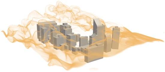
Figure 1.
Streamlines of the LES urban environment obtained using a logarithmic inlet wind profile with a reference wind speed of 8 m/s.
In prior work by the authors, the most challenging flight path within the LES domain occurred during a crosswind case at an altitude of 100 m, where the drone encountered a strong, localized high-velocity structure. This feature, illustrated in Figure 2, was selected to evaluate the aircraft’s response within both the full LES domain and its CAE reconstruction.
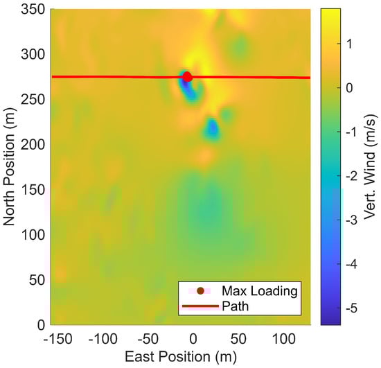
Figure 2.
Localized high-velocity structure at an altitude of 100 m within the LES domain, corresponding to the most challenging crosswind condition encountered by the drone.
To integrate the LES wind field shown in Figure 2 into the flight dynamics environment, native Simulink n-D Lookup Table blocks were implemented. These blocks require the relevant portion of the domain to be preloaded into system memory, which can substantially increase model initialization time depending on the dataset size. To mitigate this overhead, only a 40 m-thick slice centered at an altitude of 100 m was loaded into the lookup tables.
2.2.2. Convolutional Autoencoder Algorithm
Based on the current state of the art in machine learning algorithms [17,18] applied to urban wind fields, a CAE is employed to compress wind data for integration into real-time simulations. The encoder architecture of the CAE is illustrated in Figure 3, where an example with three convolutional layers is shown.
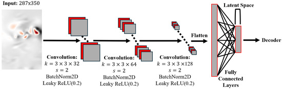
Figure 3.
The encoder structure used for data compression of the wind fields. Here, three convolutional layers are used ().
At the core of the CAE is the generation of feature maps through convolutional layers. Each convolutional layer follows three steps: a 2D convolution with 3 × 3 kernels that produces n feature maps, BatchNorm2D to normalize each feature map to zero mean and unit variance, and a LeakyReLU activation applied elementwise to introduce nonlinearity and enable complex mappings that support data compression.
The convolution step is a matrix operation that applies learnable filters, or kernels, across the spatial domain to extract localized flow structures from the data. For this application, a 3 × 3 kernel was found to work well and is thus used for all convolutional layers. The stride, which specifies how far the kernel shifts across the input, corresponds to the amount of downsampling that occurs. A stride of 2 is applied throughout the encoder to reduce spatial resolution. The number of feature maps increases with depth to maintain representational capacity. Here, the following progression is used: [32, 64, 128, 256, 512, 1024]. This is illustrated in Figure 3 where 128 feature maps are generated after three convolutional layers.
After passing through the convolutional layers, the resulting feature maps are flattened, and fully connected layers are used to map the information into a latent space of a specified size. Again, Leaky ReLU activation functions are applied. The latent space and number of convolutional layers are then selected to achieve maximum compression while maintaining sufficient fidelity in reconstruction. The process of converting the input to the reduced latent space is known as the encoder operation of the CAE and is shown in Figure 3. The decoder then performs the reverse operation to reconstruct the original wind field from the latent representation. For simplicity, the decoder is not shown, as its process is the inverse of the encoder illustrated in Figure 3.
The weights of both the fully connected layers and the convolution kernels are optimized through backpropagation using a Weighted Mean Squared Error (W-MSE) loss function as shown in Equation (13), where a of 1.0 was used. The loss function is calculated by subtracting the original wind field value (y) from the reconstructed value (), applying a weight to the difference, and then finding the average of the squared error across the entire training dataset. After training, only the latent space vector generated using the encoder and the decoder are required to represent the wind field.
The performance of CAEs is highly dependent on the network architecture and the choice of hyperparameters, which often requires an iterative trial-and-error process due to the large number of tunable parameters (e.g., kernel size, stride, number of layers, latent space dimension). A summary of the relevant hyperparameters for this architecture are given in Table 2.
Table 2.
Hyperparameters of the Convolutional Autoencoder Architecture.
In the present study, hyperparameter analysis is restricted to variations in the number of convolutional layers and the size of the latent vector, with the corresponding convergence results presented in Section 3.1. More complex CAE configurations were also examined, including architectures that employ multiple kernel sizes (3 × 3, 5 × 5, and 7 × 7) [20] and architectures based on three-dimensional kernels and latent vectors [30]. However, preliminary tests using these approaches did not produce meaningful improvements in reconstruction quality compared with the baseline architecture described above.
For completeness, reconstruction results from the multikernel autoencoder proposed in Ref. [20] are included in Section 3 to serve as a baseline for comparison with the CAE developed in this work. In implementing this multikernel architecture, BatchNorm2D and a LeakyReLU activation function were incorporated to more closely match the methodology used throughout this study.
2.3. Aerodynamic Force and Moment Generation
For this work, a sub-scale Cessna drone platform is represented in the simulation environment. A depiction of the aircraft is given in Figure 4. Assumed inertia properties and other geometric considerations that are necessary to recreate the platform are shown in Table 3.
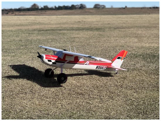
Figure 4.
Subscale Cessna drone platform.
Table 3.
Properties of subscale Cessna drone vehicle.
Two representations of the drone are evaluated. This includes the Compact Vortex Lattice Method (CVLM) that was implemented in Ref. [16] and a flight-derived state-space model of the same aircraft developed by Simmons [31] using linear regression techniques from a perturbation maneuver.
2.3.1. Compact Vortex Lattice
The Compact Vortex Lattice Method (CVLM), as described by Bunge [32], was implemented in the simulation environment for its computational efficiency and simplicity. This approach enables simulations to run faster than real time. Furthermore, only the aerodynamic surfaces need to be modeled using vortex ring singularity elements, as illustrated in Figure 5. This method relies solely on basic geometric characteristics of the platform, such as those listed in Table 3, and ignores viscous aerodynamic effects.
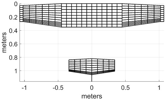
Figure 5.
Vortex lattice discretization of subscale Cessna drone in the CVLM.
Once the aerodynamic surfaces have been discretized, the matrices and are precomputed and stored, as outlined in Ref. [32]. The aerodynamic forces and moments in the body frame are then calculated using Equations (4) and (5). The state information matrix (X), which includes the body-axis velocities (V) and angular rates (), is obtained using the methodologies outlined in Section 2.2 and Section 2.3.3.
2.3.2. Flight Derived State Space Model
A model derived from flight test of the same Cessna platform derived at Virginia Tech by Simmons [31] is also evaluated during simulated flight in the reconstructed winds. In this representation, the forces and moments are determined from a state-space model whose parameters were identified using linear regression and output-error system identification methodologies [33]. The model found in Ref. [31] is implemented into the simulation environment by calculating the desired states and multiplying said states by the stability and control derivatives defined by Simmons. The convention for and the non-dimensional angular rates (,,) are given below in Equations (7) and (8).
2.3.3. Four-Point Method
Additional force and moment contributions from the methodologies described in Ref. [16] have been incorporated using the four-point method. As noted by Mohamed [34], asymmetric loading resulting from localized variations in the aerodynamic angles as the aircraft traverses a wind field can significantly impact the response of drone vehicles, particularly in the roll axis. To approximate these asymmetric effects, the four-point method is used. This method is attributed to Etkin [35] and has been demonstrated in simulation environments by Galway [36] and Cybyk [37].
The four reference locations used in the four-point method are shown in Figure 6. For a conventional fixed-wing drone configuration, the first two locations are generally aligned with the center of gravity, positioned on opposite wings, and separated by . The third point () is coincident with the center of gravity, while the fourth point () is located at roughly the quarter chord of the horizontal tail and aligned with the center of gravity. The moment arm from the center of gravity to () is defined as . These guidelines are defined this way purely for modeling convenience. As shown by Cybyk [37] for a flying wing configuration, the exact locations of the points can be modified to accommodate unconventional drone configurations.
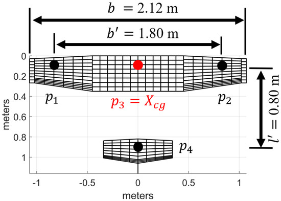
Figure 6.
Reference locations used for the four-point method.
Temporal and spatial interpolation is used to define the body wind velocities at these four reference locations. The forward (), lateral (), and vertical () body wind velocities are found at each location as specified by the subscript (e.g., the vertical velocity at station one is ). Equations (9)–(11) are then used to approximate the additional angular rate contributions associated with the wind.
The total angular velocities are found by summing the wind contributions with the angular rates associated with the vehicle, as shown in Equations (13) and (14). These outputs are then incorporated into the state matrix of the CVLM or the state-space model, and the forces and moments are updated accordingly, taking into account the asymmetric loading effects.
There are other methodologies that could be used to account for the asymmetric loadings, such as obtaining localized force and moment contributions from CFD models or through more involved vector math operations, as shown by Cybyk [37]. However, the modeling advantages of incorporating these approaches, particularly for drone vehicles, have not been thoroughly explored or validated at the time of writing and therefore remain an open area of research.
2.4. Integration Scheme to Update Drone States
The equations of motion are integrated using the 6DOF Euler attitude block from Simulink’s Aerospace Blockset. This block assumes a point mass model and requires only the vehicle’s mass, moments of inertia, and initial state conditions. At each timestep, the body-frame forces and moments computed using the methods described in Section 2.3 are provided as inputs. Simulink automatically determines the integration scheme and time step.
2.5. Control Laws for Desired Maneuvers
ArduPilot [38] is utilized for waypoint tracking and disturbance rejection within the simulation environment. Once the vehicle states are computed, they are transmitted to ArduPilot via a JSON interface over a Transmission Control Protocol (TCP) network connection [39]. ArduPilot responds with control input signals in the form of pulse-width modulation (PWM), which are then converted into commanded control surface deflections. Actuator dynamics are applied using the transfer function models listed in Table 4, as provided by Schulze et al. [40] for a representative small drone platform.
Table 4.
Actuator dynamic transfer functions.
The Autotune mode in ArduPilot is employed to tune the proportional-integral-derivative (PID) gains. In this mode, stick inputs are provided to the aircraft, and the gains are iteratively adjusted until the desired response is achieved. The target response is influenced by the AUTOTUNE_LEVEL parameter, which is set to its default value of 6 in this study, corresponding to a medium tuning level. The final PID gains obtained from the Autotune process and applied to the subscale Cessna drone are listed in Appendix A.
3. Results
3.1. CAE Hyperparameter Study
The CAEs were trained on a 40 m segment of LES wind field data centered at an altitude of 100 m. This domain was divided into 2D slices, with each slice containing 151 time samples and a domain size of 287 m × 350 m. The spatial resolution of the domain in all axes is 1 m. Some samples of the dataset at the 100 m altitude are shown in Figure 7. These 2D slices served as the training inputs for the CAEs. The size of the dataset for each wind axis is 2487.5 MB for a total of 7462.5 MB. Each axis was trained individually.
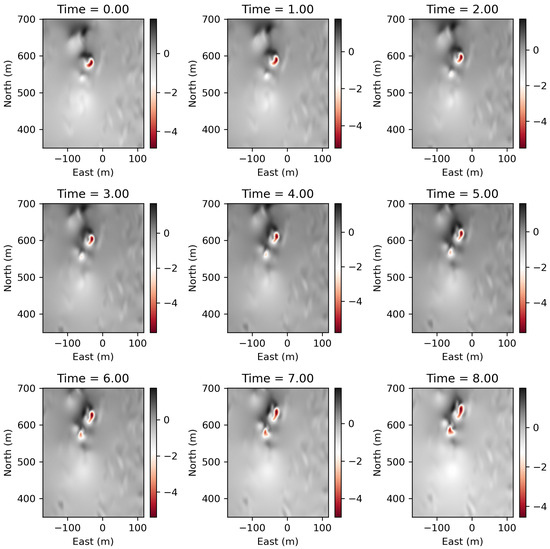
Figure 7.
Samples of the training dataset at an altitude of 100 m used to train the CAEs.
To evaluate the influence of network structure, different combinations of latent space dimensions and numbers of convolutional layers were tested, as summarized in Figure 8a. The loss function described in Equation (3) is used in Figure 8a to quantify the impact of the CAE structure. The resulting storage size required to store the weights needed for the decoder and all of the resulting latent vectors is shown in Figure 8b. This convergence study was used to identify the CAE configurations that provide the best balance between compression and reconstruction accuracy. From the results, a latent vector of 512 and 4 convolutional layers were selected for the final CAE structure.
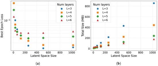
Figure 8.
Convergence study results. (a) Impact of the convolutional layers and latent space size on the loss function. (b) The resulting storage size required for the decoder weights and the latent space vectors.
3.2. Machine Learning Wind Field Representation
The three worst reconstructions of the vertical wind velocities, as measured using the MSE loss function with the finalized hyperparameters, are presented in Figure 9. The 2-D slices shown are at an altitude of 100 m, which is consistent with Figure 2. As shown, the differences between the LES wind field and the CAE representation are at most a few tenths different and are sparsely located throughout the domain. The relative difference between the two wind field representations will now be evaluated by recreating the wind structure encounter as shown in Figure 2.
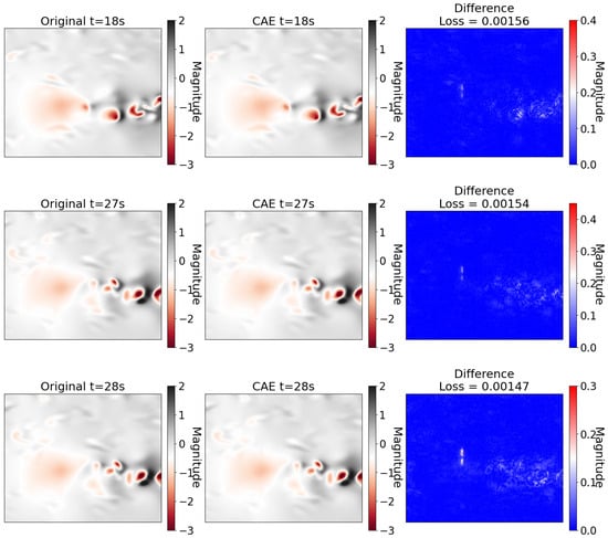
Figure 9.
The three worst reconstruction results from the CAE at an altitude of 100 m based on the loss function.
The three worst reconstructions of the vertical wind velocities using the multikernel autoencoder (MS-CAE) proposed in Ref. [20] are shown in Figure 10. Upon examining both Figure 9 and Figure 10, it is apparent that the differences using the proposed CAE are overall less than the MS-CAE proposed in the existing literature. This is further supported by Table 5, which lists the final modified MSE loss function for each methodology. For Table 5, CAE is the methodology proposed by the author’s and MS-CAE is the methodology based on Ref. [20].
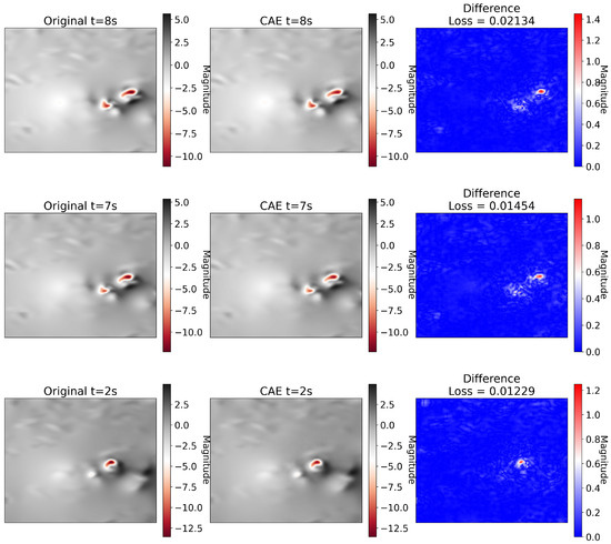
Figure 10.
The three worst reconstruction results from the proposed MS-CAE of Ref. [20] at an altitude of 100 m based on the loss function.
Table 5.
The w-mse of the two architectures for the vertical velocity fields (w) at an altitude of 100 m.
3.3. Flight Dynamics Results
After training, the CAE is able to reconstruct any 2D slice of the domain from its corresponding latent-space vector for each altitude and time sample. During simulation, the appropriate slices are reconstructed based on the drone’s position and the current simulation time. If the point of interest lies between grid nodes in the reconstructed 2D slice, or if the simulation time falls between two available samples, interpolation is used to obtain the required wind value. The resulting interpolated wind magnitudes are then given to the flight dynamics model to find the resulting influence on the vehicle’s states.
A comparison of the time histories of the states of the drone in the presence of the LES and CAE winds for the CVLM and flight-derived aerodynamic models is shown in Figure 11 and Figure 12. The drone navigates along the nominal path shown in Figure 2 and encounters the wind structure. This encounter yielded the largest acceleration magnitude at the 100 m altitude in the authors’ previous work [16].
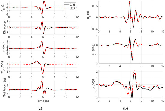
Figure 11.
Flight dynamic time histories of the drone in the LES and CAE wind fields using the CVLM aerodynamic model. is the vertical wind magnitude interpolated from the wind model. (a) Longitudinal flight dynamic time histories. (b) Lateral flight dynamic time histories.
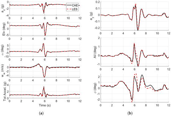
Figure 12.
Flight dynamic time histories of the drone in the LES and CAE wind fields using the flight-derived state-space model. is the vertical wind magnitude interpolated from the wind model. (a) Longitudinal flight dynamic time histories. (b) Lateral flight dynamic time histories.
4. Conclusions
This study demonstrated that a CAE can efficiently compress LES urban wind fields for real-time analysis of drone flight dynamics. A 40 m-deep LES section was reduced from 7462.5 MB to 650.6 MB, achieving a 91% reduction in storage while maintaining reconstruction errors within a few tenths of the local velocity magnitude (Figure 9). These compression gains substantially decrease initialization time and enable the use of larger simulation domains. Model training was completed in less than 30 min on a consumer-grade desktop computer (Table 1). Flight dynamics comparisons between the full LES and the CAE-reconstructed wind fields (Figure 11 and Figure 12) showed only marginal differences, confirming the framework’s suitability for real-time integration.
The maximum total acceleration predicted by the flight-derived model was 3.47 g, compared to 3.02 g for the Compact Vortex Lattice Method (CVLM). The flight-derived model also required larger elevator deflections and exhibited greater angle-of-attack () deviations, suggesting reduced disturbance rejection relative to the CVLM. These discrepancies are consistent with the known tendency of vortex-lattice–based solvers to overpredict control effectiveness due to their reliance on potential flow theory and neglect of viscous effects [41].
A further source of discrepancy is the assumed location of the center of gravity. Because Ref. [31] does not specify this parameter, the true offset between models cannot be established. To mitigate this uncertainty, the center of gravity in the CVLM model was shifted rearward until matched that of the flight-derived model (−0.32 vs. −0.30), as reported in Table 3.
Overall, these results demonstrate that CAEs provide a computationally efficient means of representing large urban wind fields while maintaining accuracy in flight dynamics predictions. In comparison to the Proper Orthogonal Decomposition (POD) reduced-order models from earlier work [10], the CAE methodology achieved significantly better performance in reproducing the flight dynamics of the full-order model. This capability enables the use of larger simulation domains, facilitates data sharing, and advances the development of robust assessment frameworks for certifying drones in complex urban environments.
5. Future Research Directions
Although the CAE methodology performed well in this study, future work should extend the approach to larger domains to evaluate whether comparable compression ratios and reconstruction accuracy can be maintained. This may require more advanced architectures, such as multi-scale kernels [20] or fully three-dimensional kernels [30]. The computational costs of training CAEs on such domains are not yet well understood. A systematic assessment of training-time scaling across multiple GPUs, along with benchmarking on successive GPU generations, would help establish practical limits of domain size and provide guidelines for efficient deployment. Additionally, the CAE framework could be further enhanced by incorporating other machine learning techniques, such as self-attention mechanisms, reinforcement learning, or physics-informed neural network strategies.
The integration between the CAE code and the Simulink environment also requires improvement. In the current implementation, the CAE was trained in PyTorch 2.6.0 and linked to MATLAB 2024b through external scripts, which introduced runtime penalties during wind-field simulations. Developing a more efficient CAE–Simulink interface, such as native MATLAB/PyTorch integration or lightweight compiled models, will be essential to achieve faster-than-real-time performance. Such advances would broaden the applicability of reduced-order modeling in flight dynamics and strengthen its role in safety assessment and certification of drones operating in complex urban environments.
Author Contributions
K.K. developed the concept and methodology for the LES wind field model. R.P. conceived the dynamic simulation experiment using a representative drone. Z.K. performed the aerodynamic modeling and flight dynamics simulation experiments. All authors have read and agreed to the published version of the manuscript.
Funding
This material is based upon work supported by the National Science Foundation under Grant No. 1925147. Any opinions, findings, and conclusions or recommendations expressed in this material are those of the authors and do not necessarily reflect the views of the National Science Foundation.
Data Availability Statement
The data supporting this study’s findings and additional details to replicate are available upon request to the corresponding author.
Acknowledgments
K.K. acknowledges support from the National Science Foundation (NSF) under Grant No. 1925147. Some of the computing for this project was performed at the High-Performance Computing Center (HPCC) at Oklahoma State University, supported, in part, through the National Science Foundation (Grant No. OAC-1531128). This work also used the Bridges2 system at the Pittsburgh Supercomputing Center (PSC) through allocation MTH220018 from the Advanced Cyberinfrastructure Coordination Ecosystem: Services & Support (ACCESS) program, which is supported by U.S. National Science Foundation grants #2138259, #2138286, #2138307, #2137603, and #2138296. Z.K. acknowledges support from the Department of Defense (DoD) SMART (Science, Mathematics, and Research for Transformation) scholarship program. The SMART scholarship is funded by: OUSD/R&E (The Under Secretary of Defense-Research and Engineering), National Defense Education Program (NDEP)/ BA-1, Basic Research.
Conflicts of Interest
The authors declare no conflicts of interest.
Appendix A
Table A1.
ArduPlane control parameters used in the simulation environment.
Table A1.
ArduPlane control parameters used in the simulation environment.
| Parameter | Value |
|---|---|
| Servo Roll PID | |
| P | 0.203 |
| I | 0.153 |
| D | 0.007 |
| INT_MAX | 0.0066 |
| Servo Pitch PID | |
| P | 1.471 |
| I | 1.103 |
| D | 0.040 |
| INT_MAX | 0.0066 |
| Servo Yaw | |
| P | 1.000 |
| I | 0.500 |
| D | 0.500 |
| INT_Max | 15.0 |
| L1 Control—Turn Control | |
| Period | 40 |
| Damping | 0.75 |
| TECS | |
| Climb Max (m/s) | 5.0 |
| Sink Min (m/s) | 2.0 |
| Sink Max (m/s) | 5.0 |
| Pitch Dampening | 0.3 |
| Time Const | 5.0 |
References
- Faithfull, M. Walmart Drone Dream Has Been Cleared For Take Off In Dallas. Available online: https://www.forbes.com/sites/markfaithfull/2024/05/13/walmart-drone-dream-has-been-cleared-for-take-off-in-dallas/ (accessed on 10 January 2024).
- Patterson, M. Advanced Air Mobility (AAM): An Overview and Brief History. In Proceedings of the SU Transportation Engineering and Safety Conference, Online, 8–10 December 2021. [Google Scholar]
- Johnson, W.; Silva, C. NASA concept vehicles and the engineering of advanced air mobility aircraft. Aeronaut. J. 2022, 126, 59–91. [Google Scholar] [CrossRef]
- Goyal, R.; Reiche, C.; Fernando, C.; Cohen, A. Advanced air mobility: Demand analysis and market potential of the airport shuttle and air taxi markets. Sustainability 2021, 13, 7421. [Google Scholar] [CrossRef]
- Goyal, R.; Cohen, A. Advanced air mobility: Opportunities and challenges deploying eVTOLs for air ambulance service. Appl. Sci. 2022, 12, 1183. [Google Scholar] [CrossRef]
- Nithya, D.; Quaranta, G.; Muscarello, V.; Liang, M. Review of wind flow modelling in urban environments to support the development of urban air mobility. Drones 2024, 8, 147. [Google Scholar] [CrossRef]
- Connors, M.M. Understanding Risk in Urban air Mobility: Moving Towards Safe Operating Standards. 2020. Available online: https://ntrs.nasa.gov/api/citations/20205000604/downloads/NASA%20TM20205000604.pdf (accessed on 10 August 2025).
- Ranquist, E.; Steiner, M.; Argrow, B. Exploring the Range of Weather Impacts on UAS Operations. In Proceedings of the 18th Conference on Aviation, Range and Aerospace Meteorology, Seattle, WA, USA, 22–26 January 2017. [Google Scholar]
- Micallef, D.; Van Bussel, G. A review of urban wind energy research: Aerodynamics and other challenges. Energies 2018, 11, 2204. [Google Scholar] [CrossRef]
- Krawczyk, Z.; Vuppala, R.K.; Paul, R.; Kara, K. Evaluating Reduced-Order Urban Wind Models for Simulating Flight Dynamics of Advanced Aerial Mobility Aircraft. Aerospace 2024, 11, 830. [Google Scholar] [CrossRef]
- Corbetta, M.; Jarvis, K.; Banerjee, P. Uncertainty propagation in pre-flight prediction of unmanned aerial vehicle separation violations. In Proceedings of the 2022 IEEE Aerospace Conference (AERO), Big Sky, MT, USA, 5–12 March 2022; IEEE: Piscataway, NJ, USA, 2022; pp. 1–11. [Google Scholar]
- Banerjee, P.; Bradner, K. Energy-Optimized Path Planning for Uas in Varying Winds Via Reinforcement Learning. In Proceedings of the AIAA Aviation Forum and ASCEND 2024, Las Vegas, NV, USA, 29 July–2 August 2024; p. 4545. [Google Scholar]
- Moore, A.J.; Young, S.; Altamirano, G.; Ancel, E.; Darafsheh, K.; Dill, E.; Foster, J.; Quach, C.; Mackenzie, A.; Matt, J.; et al. Testing of Advanced Capabilities to Enable In-Time Safety Management and Assurance for Future Flight Operations. 2024. Available online: https://ntrs.nasa.gov/api/citations/20230018665/downloads/NASA-TM-20230018665.pdf (accessed on 10 August 2025).
- Vita, G.; Shu, Z.; Jesson, M.; Quinn, A.; Hemida, H.; Sterling, M.; Baker, C. On the assessment of pedestrian distress in urban winds. J. Wind Eng. Ind. Aerodyn. 2020, 203, 104200. [Google Scholar] [CrossRef]
- Shirzadi, M.; Tominaga, Y. CFD evaluation of mean and turbulent wind characteristics around a high-rise building affected by its surroundings. Build. Environ. 2022, 225, 109637. [Google Scholar] [CrossRef]
- Krawczyk, Z.; Vuppala, R.K.; Paul, R.; Kara, K. Urban Wind Field Effects on the Flight Dynamics of Fixed-Wing Drones. Drones 2025, 9, 362. [Google Scholar] [CrossRef]
- Masoumi-Verki, S.; Haghighat, F.; Eicker, U. A review of advances towards efficient reduced-order models (ROM) for predicting urban airflow and pollutant dispersion. Build. Environ. 2022, 216, 108966. [Google Scholar] [CrossRef]
- Caron, C.; Lauret, P.; Bastide, A. Machine Learning to speed up Computational Fluid Dynamics engineering simulations for built environments: A review. Build. Environ. 2025, 267, 112229. [Google Scholar] [CrossRef]
- Clemente, A.V.; Giljarhus, K.E.T.; Oggiano, L.; Ruocco, M. Configurable convolutional neural networks for real-time pedestrian-level wind prediction in urban environments. arXiv 2023, arXiv:2311.07985. [Google Scholar]
- Masoumi-Verki, S.; Haghighat, F.; Eicker, U. Improving the performance of a CAE-based reduced-order model for predicting turbulent airflow field around an isolated high-rise building. Sustain. Cities Soc. 2022, 87, 104252. [Google Scholar] [CrossRef]
- Xiang, S.; Fu, X.; Zhou, J.; Wang, Y.; Zhang, Y.; Hu, X.; Xu, J.; Liu, H.; Liu, J.; Ma, J.; et al. Non-intrusive reduced order model of urban airflow with dynamic boundary conditions. Build. Environ. 2021, 187, 107397. [Google Scholar] [CrossRef]
- Fu, R.; Xiao, D.; Navon, I.; Wang, C. A data driven reduced order model of fluid flow by auto-encoder and self-attention deep learning methods. arXiv 2021, arXiv:2109.02126. [Google Scholar]
- Mücke, N.T.; Bohté, S.M.; Oosterlee, C.W. Reduced order modeling for parameterized time-dependent PDEs using spatially and memory aware deep learning. J. Comput. Sci. 2021, 53, 101408. [Google Scholar] [CrossRef]
- Gonzalez, F.J.; Balajewicz, M. Deep convolutional recurrent autoencoders for learning low-dimensional feature dynamics of fluid systems. arXiv 2018, arXiv:1808.01346. [Google Scholar] [CrossRef]
- Hasegawa, K.; Fukami, K.; Murata, T.; Fukagata, K. CNN-LSTM based reduced order modeling of two-dimensional unsteady flows around a circular cylinder at different Reynolds numbers. Fluid Dyn. Res. 2020, 52, 065501. [Google Scholar] [CrossRef]
- Eivazi, H.; Veisi, H.; Naderi, M.H.; Esfahanian, V. Deep neural networks for nonlinear model order reduction of unsteady flows. Phys. Fluids 2020, 32, 105104. [Google Scholar] [CrossRef]
- Beard, R.W.; McLain, T.W. Small Unmanned Aircraft: Theory and Practice; Princeton University Press: Princeton, NJ, USA, 2012. [Google Scholar]
- Jasak, H.; Jemcov, A.; Tukovic, Z. OpenFOAM: A C++ library for complex physics simulations. In Proceedings of the International Workshop on Coupled Methods in Numerical Dynamics, IUC Dubrovnik, Croatia, 19–21 September 2007; Volume 1000, pp. 1–20. [Google Scholar]
- Vuppala, R.K.; Krawczyk, Z.; Paul, R.; Kara, K. Modeling advanced air mobility aircraft in data-driven reduced order realistic urban winds. Sci. Rep. 2024, 14, 383. [Google Scholar] [CrossRef]
- Xiang, S.; Zhou, J.; Fu, X.; Zheng, L.; Wang, Y.; Zhang, Y.; Yi, K.; Liu, J.; Ma, J.; Tao, S. Fast simulation of high resolution urban wind fields at city scale. Urban Clim. 2021, 39, 100941. [Google Scholar] [CrossRef]
- Simmons, B.M.; Gresham, J.L.; Woolsey, C.A. Nonlinear dynamic modeling for aircraft with unknown mass properties using flight data. J. Aircr. 2023, 60, 968–980. [Google Scholar] [CrossRef]
- Bunge, R.; Kroo, I. Compact formulation of nonlinear inviscid aerodynamics for fixed-wing aircraft. In Proceedings of the 30th AIAA Applied Aerodynamics Conference, New Orleans, LA, USA, 25–28 June 2012; p. 2771. [Google Scholar]
- Morelli, E.A.; Klein, V. Aircraft System Identification: Theory and Practice; Sunflyte Enterprises: Williamsburg, VA, USA, 2016; Volume 2. [Google Scholar]
- Mohamed, A.; Marino, M.; Watkins, S.; Jaworski, J.; Jones, A. Gusts encountered by flying vehicles in proximity to buildings. Drones 2023, 7, 22. [Google Scholar] [CrossRef]
- Etkin, B. Dynamics of Atmospheric Flight; Courier Corporation: North Chelmsford, MA, USA, 2005. [Google Scholar]
- Galway, D.; Etele, J.; Fusina, G. Development and implementation of an urban wind field database for aircraft flight simulation. J. Wind Eng. Ind. Aerodyn. 2012, 103, 73–85. [Google Scholar] [CrossRef]
- Cybyk, B.Z.; McGrath, B.E.; Frey, T.M.; Drewry, D.G.; Keane, J.F.; Patnaik, G. Unsteady airflows and their impact on small unmanned air systems in urban environments. J. Aerosp. Inf. Syst. 2014, 11, 178–194. [Google Scholar] [CrossRef]
- ArduPilot: Github. 2024. Available online: https://github.com/ArduPilot/ardupilot (accessed on 10 August 2025).
- Eddy, W.; Mathis, M.; Duke, M. Transmission Control Protocol (TCP) Specification. Request for Comments 9293. 2022. Available online: https://www.ietf.org/rfc/rfc9293.html#name-purpose-and-scope (accessed on 2 December 2024).
- Schulze, P.C.; Miller, J.; Klyde, D.H.; Regan, C.D.; Alexandrov, N. System identification of a small UAS in support of handling qualities evaluations. In Proceedings of the AIAA Scitech 2019 Forum, San Diego, CA, USA, 7–11 January 2019; p. 0826. [Google Scholar]
- Park, S. Modeling with vortex lattice method and frequency sweep flight test for a fixed-wing UAV. Control Eng. Pract. 2013, 21, 1767–1775. [Google Scholar] [CrossRef]
Disclaimer/Publisher’s Note: The statements, opinions and data contained in all publications are solely those of the individual author(s) and contributor(s) and not of MDPI and/or the editor(s). MDPI and/or the editor(s) disclaim responsibility for any injury to people or property resulting from any ideas, methods, instructions or products referred to in the content. |
© 2025 by the authors. Licensee MDPI, Basel, Switzerland. This article is an open access article distributed under the terms and conditions of the Creative Commons Attribution (CC BY) license (https://creativecommons.org/licenses/by/4.0/).