Multi-UAV Dynamic Target Search Based on Multi-Potential-Field Fusion Reward Shaping MAPPO

Highlights

What are the main findings?

• Proposes MPRS-MAPPO, an adaptive reward shaping method integrating three potential fields, enhancing multi-UAV coordination and learning efficiency in dynamic target search.
• Achieves a 7.87–29.76% improvement in target detection rate and an 11.58% increase in training return compared to baseline methods.

What are the implications of the main findings?

• Offers an effective MARL framework for cooperative search under sparse rewards and dynamic conditions.
• The design enhances efficiency and stability, serving as a reference for other multi-agent systems.

Abstract

In the cooperative search for dynamic targets by multiple UAVs, target uncertainty and system complexity pose significant challenges to cooperative decision-making. Multi-agent reinforcement learning (MARL) technology can be used for cooperative policy optimization, but it suffers from convergence difficulties and low policy quality in reward-sparse environments such as dynamic target search. To address this issue, this paper proposes a Multi-Potential-Field Fusion Reward Shaping MAPPO (MPRS-MAPPO) algorithm. First, three potential field functions are constructed for reward shaping: probability edge potential field, maximum probability potential field, and coverage probability sum potential field. Subsequently, an adaptive fusion weight mechanism is proposed to adjust fusion weights based on the correlation between potential field values and advantage values. Furthermore, a warm-up phase is introduced to improve training stability. Extensive experiments, including multi-scale and physical tests, demonstrate that MPRS-MAPPO significantly improves convergence speed, detection rate, and stability compared with MAPPO, MASAC, QMIX, and Scanline. Detection rates increased by 7.87–29.76%, and training uncertainty decreased by 7.43–56.36%, validating the algorithm’s robustness, scalability, and real-world applicability.

1. Introduction

Unmanned aerial vehicles (UAVs), owing to their cost-effectiveness, flexible deployment, and adaptability to complex environments, have been extensively employed in tasks such as reconnaissance, mapping, patrolling, and target search, becoming indispensable components of intelligent perception systems [1,2]. In multi-UAV systems, these advantages are further amplified: cooperative operations not only enhance the efficiency and robustness of complex task execution but also expand mission coverage and system scalability [3]. In particular, for dynamic target search missions in unknown environments, multi-UAV systems have been widely applied in disaster rescue, agricultural inspection, and counter-terrorism security scenarios [4,5].

Nevertheless, multi-UAV systems still encounter considerable challenges in dynamic target search tasks. On one hand, their cooperative mechanisms are inherently complex, requiring rational task allocation to avoid path conflicts, resource waste, and redundant search efforts. On the other hand, targets generally possess only limited prior location information at the initial stage, and their positions and movements change over time, which makes cooperative decision-making even more challenging.

Existing studies on multi-UAV dynamic target search can be broadly categorized into four methodological classes: planning-based approaches, optimization-based approaches, heuristic methods, and reinforcement learning. Planning-based methods generate high-coverage search paths through area partitioning [6,7] and trajectory design [8,9,10,11], which are suitable for static or partially known environments but lack responsiveness under dynamic target scenarios. Optimization-based approaches rely on multi-objective function models to balance metrics such as path length [12,13], search time [14,15,16], and coverage rate [17]; although theoretically optimal, their computational complexity escalates rapidly with task scale, limiting real-time applicability. Heuristic methods, including particle swarm optimization [18,19], ant colony algorithms [20], and multi-population cooperative coevolution [21], exhibit strong global search capability and algorithmic flexibility [22,23], but often lack effective feedback control, making them prone to local optima and slow convergence.

Among the aforementioned approaches, reinforcement learning (RL) [24], particularly multi-agent reinforcement learning (MARL) [25], has emerged as a promising paradigm for addressing dynamic target search problems. Its key advantage lies in its independence from precise modeling, instead enabling adaptive policy learning through continuous interaction with the environment, thereby ensuring strong generalization and robustness. In particular, multi-agent algorithms based on proximal policy optimization, such as MAPPO [26], have demonstrated remarkable performance in handling partial observability, high-dimensional state spaces, and cooperative decision-making, and have been widely applied to multi-UAV cooperative search tasks [27,28,29]. For instance, Refs. [30,31] leveraged MARL to optimize search path allocation and real-time response mechanisms, significantly improving target-tracking accuracy and system-level coordination. In scenarios with unknown target quantities or incomplete information, Ref. [32] integrated map construction with policy learning, enabling UAVs to iteratively update environmental cognition and dynamically adapt strategies during search. Furthermore, researchers have proposed various enhancements in algorithmic structures and optimization processes to further improve training stability and efficiency [33,34,35,36]. More recent studies have introduced MASAC [37] to enhance learning stability and generalization in UAV swarm decision-making under incomplete information and HAPPO [38] to improve coordination and optimization efficiency in heterogeneous multi-agent environments.

Despite the great potential of RL in this domain, its training process remains constrained by the sparse-reward problem [39]. Before the discovery of targets, agents often fail to obtain effective reward signals, leading to inefficient policy optimization. To address this challenge, researchers have introduced reward shaping (RS) techniques [40], which leverage prior knowledge to design auxiliary rewards that improve training efficiency and policy quality. Among them, potential-based reward shaping (PBRS) [41] has been widely adopted due to its provable policy invariance. Various studies have attempted to design diverse potential functions to enhance learning across different tasks. For example, energy-aware shaping functions have been used to improve UAV emergency communication efficiency [42]; position-constrained functions have been applied to optimize multi-agent assembly tasks [43]; linearly weighted multi-potential fusion has been employed to enhance single-agent adaptability [44]; and dynamic adjustment of shaping reward magnitudes has been proposed to improve stage-wise training adaptability [45]. However, in multi-agent scenarios—particularly in multi-UAV dynamic target search—systematic studies on how to effectively integrate multiple potential functions for reward shaping are still lacking.

To address these challenges, we propose a Multi-Potential-Field Fusion Reward Shaping MAPPO (MPRS-MAPPO). Building upon sparse primary rewards, this method designs three semantically meaningful potential functions that serve as shaping signals. Moreover, an adaptive fusion weight mechanism is introduced to adaptively adjust the weights of different potential functions according to their relationship with advantage values, thereby mitigating potential interference.

Table 1. Comparison of related studies.

Study	Multi-UAV	Dynamic Target	Reward Shaping	Fusion Shaping
Planning-based [6,7,8,9,10,11]	full	low	none	none
Optimization-based [12,13,14,15,16,17]	full	middle	none	none
Heuristic-based [18,19,20,21,22,23]	full	middle	none	none
RL-based [27,28,29,30,31,32,33,34,35,36]	full	full	low	none
Reward shaping [39,40,41,42,43,44,45]	low	none	full	low
This work	full	full	full	full

Full: fully supported; middle: moderately supported; low: weakly supported; none: not supported.

compares the proposed approach with existing methods across four dimensions: multi-UAV applicability, dynamic target handling, reward shaping, and potential-field fusion. It can be observed that this work is the first to integrate all four key characteristics into a unified algorithmic framework.

In summary, the main contributions of this work are as follows:

• We designed three semantically distinct potential field functions: Probability Edge Potential Field, Maximum Probability Potential Field, and Coverage Probability Sum Potential Field, which provide shaping signals from the perspectives of local prior information, global optimal prediction, and swarm-level coordination.
• We developed an Adaptive Fusion Weight Mechanism that adaptively adjusts the weights of potential functions based on their correlation with advantage values, reducing interference among multiple potentials and enabling stable and efficient training convergence.
• We proposed the MPRS-MAPPO algorithmic framework, which introduces a warm-up phase followed by a multi-potential field fusion reward shaping mechanism to address the sparse-reward challenge, thereby improving the learning efficiency and cooperation of agents in dynamic target search tasks.

Finally, extensive experiments were conducted on a custom-built multi-UAV simulation platform to validate the superiority of the proposed method in terms of training efficiency, policy coordination, and search performance.

The remainder of this paper is organized as follows. Section 2 formulates the mathematical model of the multi-UAV dynamic target search problem. Section 3 presents the proposed MPRS-MAPPO algorithm in detail. Section 4 describes the experimental design and evaluation results. Section 5 concludes the paper and outlines future research directions.

2. System Modeling

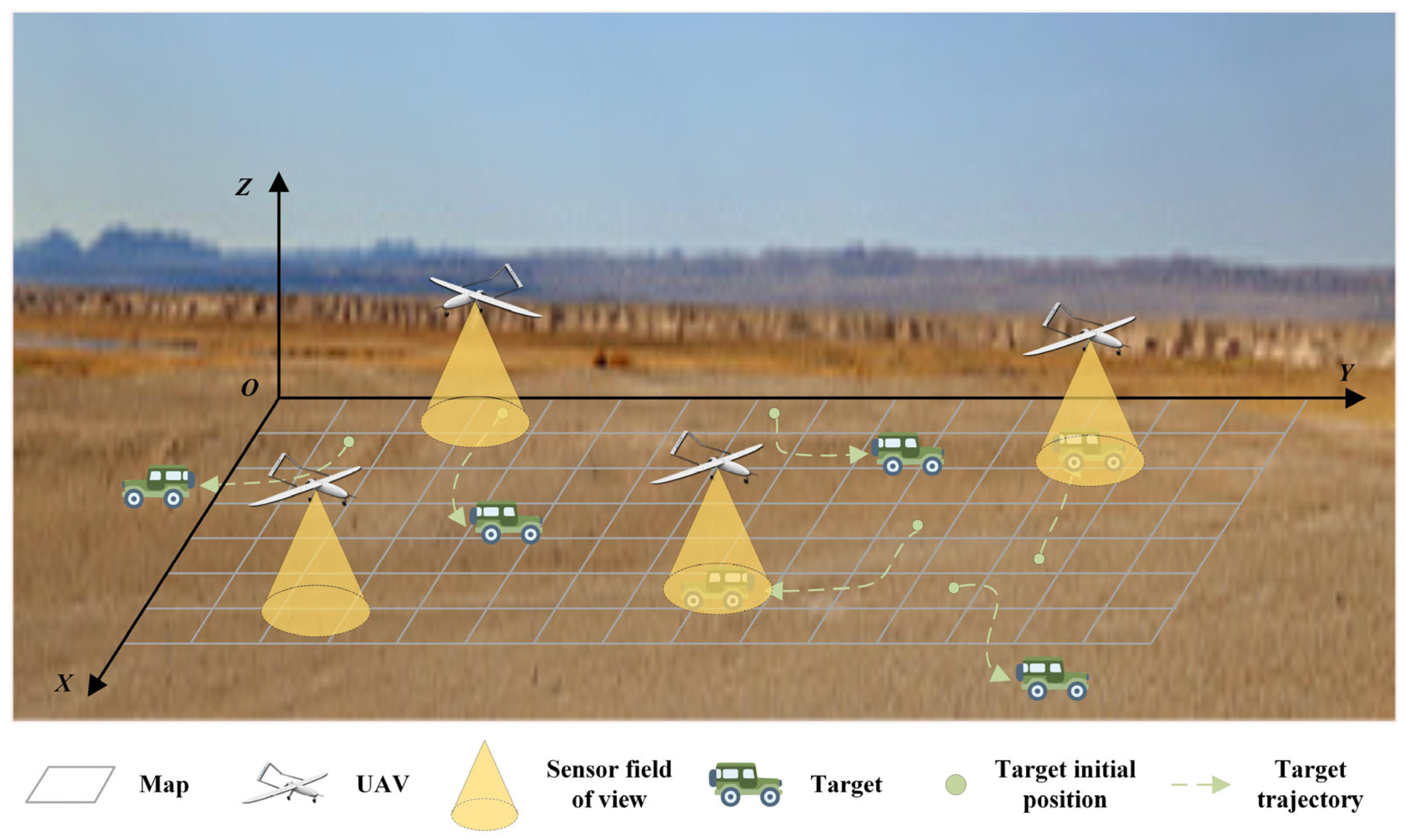
This paper investigates the cooperative search for dynamic ground targets by multiple fixed-wing UAVs. As shown in Figure 1, the task area is the ground space area. Each UAV is equipped with a sensor that has a limited field of view, the range of which is represented by a yellow cone. The ground target and its trajectory are indicated by green icons, and its movement is non-deterministic and may maneuver out of the task area. Although the UAV obtains the prior initial position of the target, the actual position of the target will continue to change due to its maneuverability. Consequently, a cooperative search by multiple UAVs is required to increase the target detection probability. The mission objective is to maximize the number of detected targets within the specified search duration.

Based on the task scenario, this section defines the environmental, target motion, UAV motion, and sensor models that provide the basis for the subsequent method research.

2.1. Environment Model

The search environment is modeled as a two-dimensional grid map $\mathcal{M}$, where the probability of a target existing at position $\mathbf{g}=(x,y)$ changes dynamically at each time step $t$. This dynamic likelihood is represented by the target probability distribution map $p\left(\mathbf{g},t\right)$, and can be expressed as follows:

$$p\left(\mathbf{g},t\right)\in \left[\mathrm{0,1}\right],\forall \mathbf{g}\in \mathcal{M}.$$

(1)

The sum of the existence probabilities of the target at each position in the area is defined as the overall existence probability of the target, and its calculation formula is as follows:

$$p_{\mathrm{r}\mathrm{e}\mathrm{m}\mathrm{a}\mathrm{i}\mathrm{n}}(t)={\sum }_{\mathbf{g}\in \mathcal{M}}p(\mathbf{g},t),$$

(2)

when $p_{\mathrm{r}\mathrm{e}\mathrm{m}\mathrm{a}\mathrm{i}\mathrm{n}}\left(t\right)$ equals 1, it indicates that the target is still within the search area; if the value is less than 1, it indicates that the target may have escaped from the area.

The UAV moves in the area, and the sensor carried by it senses a sub-area at each moment. The output of each sensing is $z\in \{0,1\}$, where $z=1$ indicates that the target is detected, otherwise it indicates that the target is not detected. For the airborne sensor, when the UAV position ${\mathbf{q}}^{\mathrm{u}\mathrm{a}\mathrm{v}}\left(t\right)$ and the target position ${\mathbf{q}}^{\mathrm{t}\mathrm{g}\mathrm{t}}\left(t\right)$ coincide, the probability of sensing the target is the detection probability $p_D$. When the UAV position ${\mathbf{q}}^{\mathrm{u}\mathrm{a}\mathrm{v}}\left(t\right)$ and the target position ${\mathbf{q}}^{\mathrm{t}\mathrm{g}\mathrm{t}}\left(t\right)$ do not coincide, the probability of misjudging the existence of the target is the false alarm probability $p_{FA}$. The details are as follows:

$$\left\{\begin{array}{c}\begin{array}{c}{p}_D=P(z=1\mid {\mathbf{q}}^{\mathrm{u}\mathrm{a}\mathrm{v}}(t)={\mathbf{q}}^{\mathrm{t}\mathrm{g}\mathrm{t}}(t))\\ p_{FA}=P(z=1\mid {\mathbf{q}}^{\mathrm{u}\mathrm{a}\mathrm{v}}(t)\ne {\mathbf{q}}^{\mathrm{t}\mathrm{g}\mathrm{t}}(t))\end{array}\end{array}\right..$$

(3)

According to the Bayesian theory and the observation results at the current moment, the posterior probability of each sub-area in the target probability distribution map can be updated. Since the movement of the target will cause the change in the overall existence probability $p_{\mathrm{r}\mathrm{e}\mathrm{m}\mathrm{a}\mathrm{i}\mathrm{n}}\left(t\right)$, it needs to be taken into account when calculating the posterior probability. Based on the probability distribution at time $t$, the probability at time $t+1$ is updated as:

$$p(\mathbf{g},t+1)=\left\{\begin{array}{c}{p}_{\mathrm{r}\mathrm{e}\mathrm{m}\mathrm{a}\mathrm{i}\mathrm{n}}(t)\cdot {\displaystyle \frac{p_D\cdot p(\mathbf{g},t)}{p_D\cdot p(\mathbf{g},t)+p_{FA}\cdot (1-p(\mathbf{g},t))}},z=1\\ p_{\mathrm{r}\mathrm{e}\mathrm{m}\mathrm{a}\mathrm{i}\mathrm{n}}(t)\cdot {\displaystyle \frac{(1-p_D)\cdot p(\mathbf{g},t)}{(1-p_D)\cdot p(\mathbf{g},t)+(1-p_{FA})\cdot (1-p(\mathbf{g},t))}},z=0\end{array}\right..$$

(4)

If there are multiple targets in the area, each target $j$ corresponds to a target probability map $p^j(\mathbf{g},t)$, which is used to represent the probability distribution of the target position in the area.

2.2. Target and UAV Motion Models

2.2.1. Target Motion Model

In this paper, multiple dynamic targets are considered, and the total number is $N_T$. For each target, only its initial position is known, while its subsequent positions evolve randomly over time. The behavior of an individual target can be modeled as a Markov process, and its probability distribution evolves accordingly. The specific formula for a single target is:

$$p(\mathbf{g},t+1)=\sum _{{\mathbf{g}}^{\prime }\in \mathcal{N}(\mathbf{g})}T({\mathbf{g}}^{\prime }\to \mathbf{g})\cdot p({\mathbf{g}}^{\prime },t),$$

(5)

in this equation, $\mathbf{g}$ and ${\mathbf{g}}^{\prime }$ denote target position, $T({\mathbf{g}}^{\prime }\to \mathbf{g})$ is the state transition probability from position ${\mathbf{g}}^{\prime }$ to $\mathbf{g}$, and $\mathcal{N}(\mathbf{g})$ is the set of neighboring grid cells reachable from ${\mathbf{g}}^{\prime }$ in a single time step. In the absence of prior information on the target’s kinematics, the transition probability $T({\mathbf{g}}^{\prime }\to \mathbf{g})$ is assumed to follow a uniform distribution. As the complexity of the target motion model increases, the position probability distribution becomes more dispersed and irregular, which makes it more difficult to discover targets within a limited time. This increased complexity also affects the convergence and stability of the cooperative search strategy. Therefore, the selection of an appropriate motion model should comprehensively consider both the characteristics of targets in specific scenarios and the computational efficiency of probabilistic inference. This paper assumes the target has a tendency to move away from its initial position. Consequently, its probability distribution spreads outwards over time, forming an annular area of high probability.

2.2.2. UAV Motion Model

This paper considers a swarm of $N_a$ homogeneous fixed-wing UAVs, represented as:

$$\mathcal{U}=\{\mathrm{u}\mathrm{a}{\mathrm{v}}_1,\mathrm{u}\mathrm{a}{\mathrm{v}}_2,\cdots ,\mathrm{u}\mathrm{a}{\mathrm{v}}_{N_a}\}.$$

(6)

Each UAV can autonomously adjust its heading and speed, and fly at different altitudes to avoid collisions. For the convenience of modeling and simulation, it is simplified into a particle model with direction constraints in a two-dimensional plane, and its state is represented by a three-dimensional vector $\left(x,y,\psi \right)$, where $\left(x,y\right)$ represents the position coordinates of the UAV in the two-dimensional plane, and $\psi$ represents its yaw angle. The continuous time motion model of the UAV is:

$$\left\{\begin{array}{c}\dot{x}=v\cos \psi \\ \dot{y}=v\sin \psi \\ \dot{\psi }=\omega \end{array}\right..$$

(7)

Discretizing this model with a sampling time of $∆t$ yields the following discrete-time model:

$$\left[\begin{array}{c}{x}_{t+1}\\ y_{t+1}\\ {\psi }_{t+1}\end{array}\right]=\left[\begin{array}{c}{x}_t\\ y_t\\ {\psi }_t\end{array}\right]+∆t\left[\begin{array}{cc}\cos {\psi }_t& 0\\ \sin {\psi }_t& 0\\ 0& 1\end{array}\right]\left[\begin{array}{c}{v}_t\\ {\omega }_t\end{array}\right].$$

(8)

To reflect the kinematic constraints of fixed-wing UAVs, this paper sets the yaw change within each time step to be $\left\{0°,\pm 45°,\pm 90°\right\}$. The UAV’s speed is normalized such that in one time step, it moves one grid unit for axial movements and $\sqrt{2}$ grid units for diagonal movements.

2.3. Sensor Model

To search for ground targets, the UAV is equipped with sensors with detection capabilities. Considering the errors in the actual sensors, the detection probability model and the false alarm probability model are established for the sensors, and the target recognition and judgment method based on the sensor model is designed.

For the detection probability model $p_D$, let the position of the UAV be ${\mathbf{q}}_i^{\mathrm{u}\mathrm{a}\mathrm{v}}\left(t\right)=\left(x_i\left(t\right),y_i\left(t\right)\right)$, the position of the point to be detected be ${\mathbf{q}}_j^{\mathrm{t}\mathrm{g}\mathrm{t}}\left(t\right)=\left(x_j\left(t\right),y_j\left(t\right)\right)$, and the detection probability decays exponentially with distance, as defined below:

$$p_D({\mathbf{q}}_j^{\mathrm{t}\mathrm{g}\mathrm{t}},{\mathbf{q}}_i^{\mathrm{u}\mathrm{a}\mathrm{v}})=p_{\mathrm{m}\mathrm{a}\mathrm{x}}\cdot e^{-d({\mathbf{q}}_j^{\mathrm{t}\mathrm{g}\mathrm{t}},{\mathbf{q}}_i^{\mathrm{u}\mathrm{a}\mathrm{v}})/\lambda },$$

(9)

where $d({\mathbf{q}}_j^{\mathrm{t}\mathrm{g}\mathrm{t}},{\mathbf{q}}_i^{\mathrm{u}\mathrm{a}\mathrm{v}})=\sqrt{(x_j-x_i{)}^2+(y_j-y_i{)}^2}$ is the Euclidean distance between the target and the sensor, $p_{\mathrm{m}\mathrm{a}\mathrm{x}}$ is the maximum detection probability when the target is at the center of the sensor’s field of view, and $\lambda$ is the attenuation coefficient. The smaller the $\lambda$, the faster the detection probability decreases.

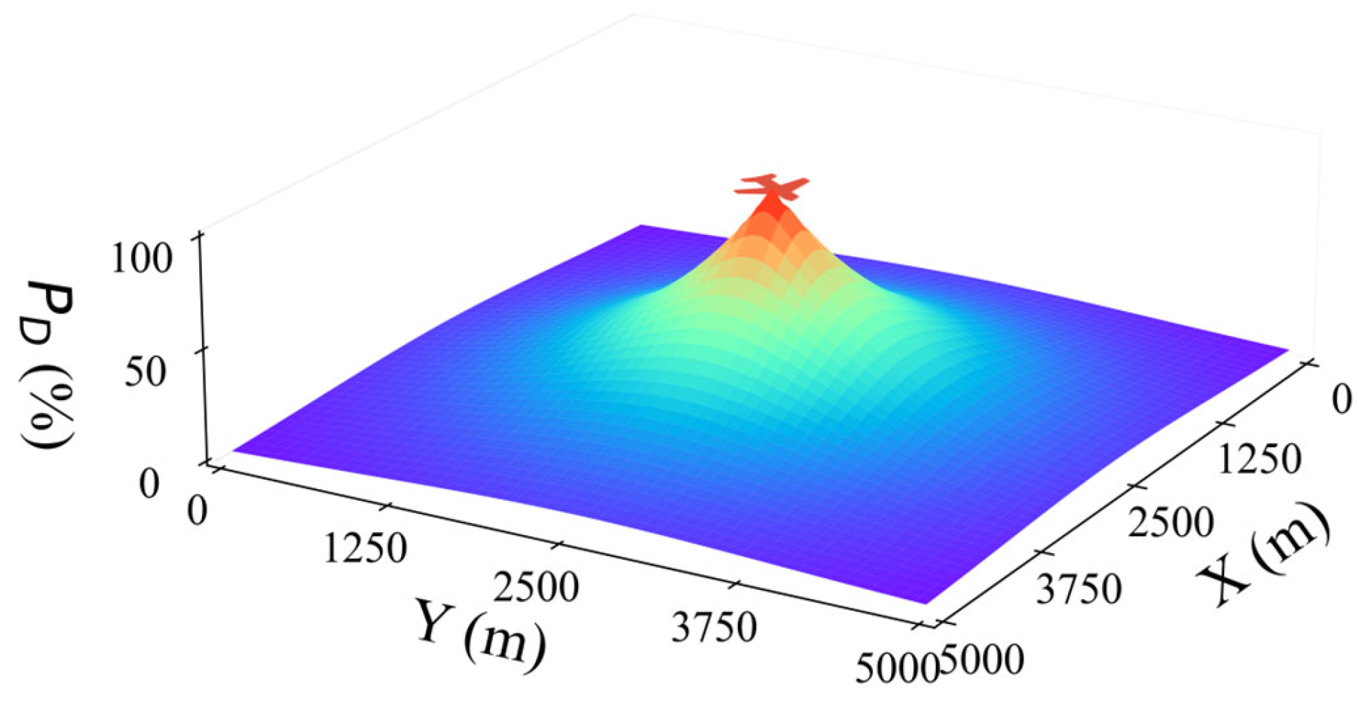
The trend of the sensor’s detection probability with distance is shown in the figure. The farther the distance from the airborne sensor, the lower the detection probability, as shown in Figure 2. In the actual simulation, the minimum effective detection probability is set to define the effective detection range of the sensor.

The false alarm probability $p_{FA}$, is the probability that the sensor incorrectly reports a target at the position where none is present. Each false alarm means that the target does not exist, but the sensor thinks it has identified the target.

From the above analysis, it can be seen that there are two possibilities for whether there is a target at the specific position $\mathbf{g}$, $\left\{H_0,H_1\right\}$, where $H_0$ indicates that there is no target at the position, and $H_1$ indicates that there is a target at the position. The sensor output is a Bernoulli variable $z\in \left[0,1\right]$, where $z=1$ indicates that the target is detected.

According to Bayes’ theorem, given a prior probability of target presence $p\left(\mathbf{g},t\right)$, the posterior probability after receiving an observation $z$ can be computed using the detection probability $p_D$, false alarm probability $p_{FA}$, and the prior probability, as follows:

$$P(H_1|z=1)={\displaystyle \frac{p_D\cdot p(\mathbf{g},t)}{p_D\cdot p(\mathbf{g},t)+p_{FA}\cdot (1-p(\mathbf{g},t))}}.$$

(10)

The method of judging whether there is a target at the point when the sensor outputs $z=1$ by setting the posterior probability threshold ${\eta }_{\mathrm{e}\mathrm{x}\mathrm{i}\mathrm{s}\mathrm{t}}$ is:

$$z_{\mathrm{j}\mathrm{u}\mathrm{d}\mathrm{g}\mathrm{e}}=\left\{\begin{array}{c}1,P\left(H_1|z=1\right)⩾{\eta }_{\mathrm{e}\mathrm{x}\mathrm{i}\mathrm{s}\mathrm{t}}\\ 0,P\left(H_1|z=1\right)<{\eta }_{\mathrm{e}\mathrm{x}\mathrm{i}\mathrm{s}\mathrm{t}}\end{array}\right.,$$

(11)

where ${\eta }_{\mathrm{e}\mathrm{x}\mathrm{i}\mathrm{s}\mathrm{t}}$ is the set posterior probability threshold, which affects the value of $z_{\mathrm{j}\mathrm{u}\mathrm{d}\mathrm{g}\mathrm{e}}$. When $z_{\mathrm{j}\mathrm{u}\mathrm{d}\mathrm{g}\mathrm{e}}$ is 1, it indicates that there is a target at this place, and when $z_{\mathrm{j}\mathrm{u}\mathrm{d}\mathrm{g}\mathrm{e}}$ is 0, it indicates that there is no target at this place.

3. Proposed Methodology

The problem of multi-UAV cooperative search for dynamic targets must account for target mobility and a finite task time, during which targets may escape the search area. The objective for the UAV cluster is to maximize the number of targets detected before they escape. Accordingly, the task objective function in this paper is formulated with two components: maximizing the number of targets detected within the mission timeframe and minimizing the sum of the initial detection times for all targets. The objective function is expressed as follows:

$$\mathrm{m}\mathrm{a}\mathrm{x}\left[{\sum }_{j=1}^{N_T}\mathbb{I}\left(t_j^{\mathrm{d}\mathrm{e}\mathrm{t}\mathrm{e}\mathrm{c}\mathrm{t}}⩽T_{\mathrm{m}\mathrm{a}\mathrm{x}}\right)-{\sum }_{j=1}^{N_T}{t}_j^{\mathrm{d}\mathrm{e}\mathrm{t}\mathrm{e}\mathrm{c}\mathrm{t}}\right],$$

(12)

where $\mathbb{I}\left(\cdot \right)$ is the indicator function, which outputs 1 when the target is detected, otherwise it is 0. $t_j^{\mathrm{d}\mathrm{e}\mathrm{t}\mathrm{e}\mathrm{c}\mathrm{t}}$ represents the time when the $j$-th target is detected; $T_{\mathrm{m}\mathrm{a}\mathrm{x}}$ is the maximum time limit of the task.

Throughout the mission, targets move randomly, their positions evolving over time, with the possibility of exiting the search area. To model this dynamic behavior, the target position constraint is defined as:

$${\mathbf{q}}_j^{\mathrm{t}\mathrm{g}\mathrm{t}}\left(t+1\right)\ne {\mathbf{q}}_j^{\mathrm{t}\mathrm{g}\mathrm{t}}\left(t\right),\forall j.$$

(13)

The mission duration for each UAV is constrained by $T_{\mathrm{m}\mathrm{a}\mathrm{x}}$, and can be expressed as follows:

$$t_i^{\mathrm{m}\mathrm{i}\mathrm{s}\mathrm{s}\mathrm{i}\mathrm{o}\mathrm{n}}⩽T_{\mathrm{m}\mathrm{a}\mathrm{x}},\forall i.$$

(14)

The UAV is subject to its own kinematic constraints, and the change rate of heading angle is limited, and can be expressed as follows:

$$\left|{\psi }_i\left(t+1\right)-{\psi }_i\left(t\right)\right|⩽\mathsf{\Delta }{\psi }_{\mathrm{m}\mathrm{a}\mathrm{x}}.$$

(15)

The position of the drone needs to meet the constraint that the position is within the map, and can be expressed as follows:

$${\mathbf{q}}_i^{\mathrm{u}\mathrm{a}\mathrm{v}}\left(t\right)\in {\mathcal{M}}_{\mathrm{m}\mathrm{i}\mathrm{s}\mathrm{s}\mathrm{i}\mathrm{o}\mathrm{n}},\forall i,t.$$

(16)

In summary, the mathematical model of the multi-UAV cooperative search problem for dynamic targets can be formally expressed as follows. This model captures the key aspects of the task, including the need to maximize the total number of targets detected within the limited mission time, as well as to minimize the cumulative initial detection times for all targets. Additionally, it incorporates several practical constraints that each UAV must satisfy during operation. These include kinematic constraints such as the maximum allowable change in heading angle, spatial constraints ensuring that UAV positions remain within the mission area, temporal constraints limiting the mission duration, and dynamic constraints reflecting the random movement of targets over time. By integrating the objective function with these constraints, the multi-UAV cooperative search problem is fully formulated as:

$$\left\{\begin{array}{c}\max \left[\sum _{j=1}^{N_T}\mathbb{I}(t_j^{\mathrm{d}\mathrm{e}\mathrm{t}\mathrm{e}\mathrm{c}\mathrm{t}}\le T_{\mathrm{m}\mathrm{a}\mathrm{x}})-\sum _{j=1}^{N_T}{t}_j^{\mathrm{d}\mathrm{e}\mathrm{t}\mathrm{e}\mathrm{c}\mathrm{t}}\right]\\ \mathrm{s}.\mathrm{t}.\\ |{\psi }_i(t+1)-{\psi }_i(t)|\le ∆{\psi }_{\mathrm{m}\mathrm{a}\mathrm{x}}\\ {\mathbf{q}}_j^{\mathrm{t}\mathrm{g}\mathrm{t}}(t+1)\ne {\mathbf{q}}_j^{\mathrm{t}\mathrm{g}\mathrm{t}}(t),\forall j\\ {\mathbf{q}}_i^{\mathrm{u}\mathrm{a}\mathrm{v}}(t)\in {\mathcal{M}}_{\mathrm{m}\mathrm{i}\mathrm{s}\mathrm{s}\mathrm{i}\mathrm{o}\mathrm{n}}\\ t_i^{\mathrm{m}\mathrm{i}\mathrm{s}\mathrm{s}\mathrm{i}\mathrm{o}\mathrm{n}}\le T_{\mathrm{m}\mathrm{a}\mathrm{x}},\forall i\end{array}\right..$$

(17)

This optimization problem is characterized by multiple objectives, numerous constraints, and stochastic target motion, making it intractable for traditional methods. To address this challenge, this paper proposes the MPRS-MAPPO algorithm for solving based on the decentralized partially observable Markov decision process (Dec-POMDP) framework and the multi-agent proximal policy optimization (MAPPO) algorithm.

3.1. Dec-POMDP Formulation

According to the characteristics of the task, the process of multi-UAV cooperative search for dynamic targets is modeled as a Dec-POMDP [30]. In this model, the global state $s_t$ cannot be perceived by a single UAV. Each UAV takes action $a_t^i$ based on its local observation information $o_t^i$. Since the target motion is unknown and each UAV can only obtain partial information, the system is partially observable. The corresponding Dec-POMDP can be described by the following tuple:

$$\langle \mathcal{N},\mathcal{S},\mathcal{A},\mathcal{T},\mathit{R},\mathsf{\Omega },\mathcal{O},\gamma \rangle ,$$

(18)

where

(1)

$\mathcal{N}=\{1,\dots ,N_a\}$ is the set of $N_a$ agents.

(2)

$\mathcal{S}$ is the state space of the global environment, and $s\in \mathcal{S}$ represents the current state.

(3)

$\mathcal{A}={\mathcal{A}}_1\times {\mathcal{A}}_2\times \cdots \times {\mathcal{A}}_{N_a}$ is the joint action space, and ${\mathcal{A}}_i$ is the action space of the $i$-th agent.

(4)

$\mathcal{T}(s^{\prime }|s,\mathbf{a})=P(s^{\prime }|s,\mathbf{a})\in \left[\mathrm{0,1}\right]$ is the state transition probability function of the environment, which represents the probability of the environment transitioning to the state $s^{\prime }$ under the state $s$ and the given joint action $\mathbf{a}=(a_1,a_2,\cdots ,a_{N_a})$ of the agent.

(5)

$\mathbf{R}(s,\mathbf{a})=(R_1(s,\mathbf{a}),R_2(s,\mathbf{a}),\cdots ,R_{N_a}(s,\mathbf{a}))$ is the joint reward function that outputs the reward values of each agent according to the current state $s$ of the environment and the joint action $\mathbf{a}$ of $N_a$ agents, where $R_i(s,\mathbf{a})$ is the reward value obtained by the $i$-th agent.

(6)

$\mathsf{\Omega }={\mathsf{\Omega }}_1\times {\mathsf{\Omega }}_2\times \cdots \times {\mathsf{\Omega }}_{N_a}$ is the observation space of $N_a$ agents, where $o_i\in {\mathsf{\Omega }}_i$ is the specific observation of the $i$-th agent.

(7)

$\mathcal{O}(s,i)$ is the local observation function, and $o_i=\mathcal{O}(s,i)$ represents the local observation $o_i$ obtained by the $i$-th agent based on the observation function in the state $s$.

(8)

$\gamma$ is the discount factor in the Markov decision process.

At time $t$, each agent $i$ obtains its own local observation result $o_t^i=\mathcal{O}(s_t,i)$ according to its own local observation function, where the global state $s_t$ is the current state of the environment that the agent cannot fully perceive. Based on $o_t^i$, each agent generates an action $a_t^i={\pi }_i(o_t^i)$ according to its policy ${\pi }_i$. The actions output by all agents constitute the joint action ${\mathbf{a}}_t=(a_t^1,a_t^2,\cdots ,a_t^{N_a})$. The environment transitions to the new state $s_{t+1}$ according to the current state $s_t$, the current joint action ${\mathbf{a}}_t$ and the state transition function $\mathcal{T}$. The environment also outputs the reward values obtained by each agent according to the joint reward function $\mathbf{R}$. The goal of each agent is to maximize the cumulative discounted reward ${\mathbb{E}}_{\mathsf{\pi }}\left[\sum _{t=0}^{\mathrm{\infty }}{\gamma }^t{R}_i(s_t,{\mathbf{a}}_t)\right]$ of all agents by optimizing the joint policy $\mathsf{\pi }=({\pi }_1,{\pi }_2,\cdots ,{\pi }_{N_a})$. The optimized policy enables the UAV to have the ability to search for cooperative dynamic targets.

3.2. State Space and Action Space

Based on the Dec-POMDP framework, $N_a$ UAVs are modeled as a multi-agent system to cooperatively search for $N_T$ potential targets. The global state $s_t\in \mathcal{S}$ contains the position and heading information of all agents, as well as the probability distribution information of all targets:

$$s_t=\left({\left\{{\mathbf{q}}_i^{\mathrm{u}\mathrm{a}\mathrm{v}}(t),{\psi }_i(t)\right\}}_{i=1}^{N_a},{\left\{{\mathcal{G}}_j,{\mathcal{P}}_j\right\}}_{j=1}^{N_T}\right),$$

(19)

where ${\mathbf{q}}_i^{\mathrm{u}\mathrm{a}\mathrm{v}}(t)=(x_i(t),y_i(t))$ denotes the grid position of agent $i$ and ${\psi }_i(t)$ is its heading. ${\mathcal{G}}_j=\{{\mathbf{g}}_{j,1},{\mathbf{g}}_{j,2},\dots ,{\mathbf{g}}_{j,M_j}\}$ is the set of grid position where the existence probability for target $j$ is non-zero, and ${\mathcal{P}}_j=\{p({\mathbf{g}}_{j,1}),p({\mathbf{g}}_{j,2}),\dots ,p({\mathbf{g}}_{j,M_j})\}$ is the set of corresponding probability values.

Due to the partial observability of the environment, agent $i$’s local observation $o_t^i\in {\mathsf{\Omega }}_i$ comprises only its own kinematic state and the local target probability map it maintains:

$$o_t^i=\left({\mathbf{q}}_i^{\mathrm{u}\mathrm{a}\mathrm{v}}(t),{\psi }_i(t),{\left\{{\mathcal{G}}_j^i,{\mathcal{P}}_j^i\right\}}_{j=1}^{N_T}\right),$$

(20)

where ${\mathcal{G}}_j^i$ and ${\mathcal{P}}_j^i$ represent the estimation of the probability area position and probability value of target $j$ by agent $i$ respectively. In this implementation, the global state is constructed by aggregating all agents’ local observations.

The discrete action space ${\mathcal{A}}_i$ for each agent $i$ is defined as:

$${\mathcal{A}}_i=\{a_1,a_2,a_3,a_4,a_5\},$$

(21)

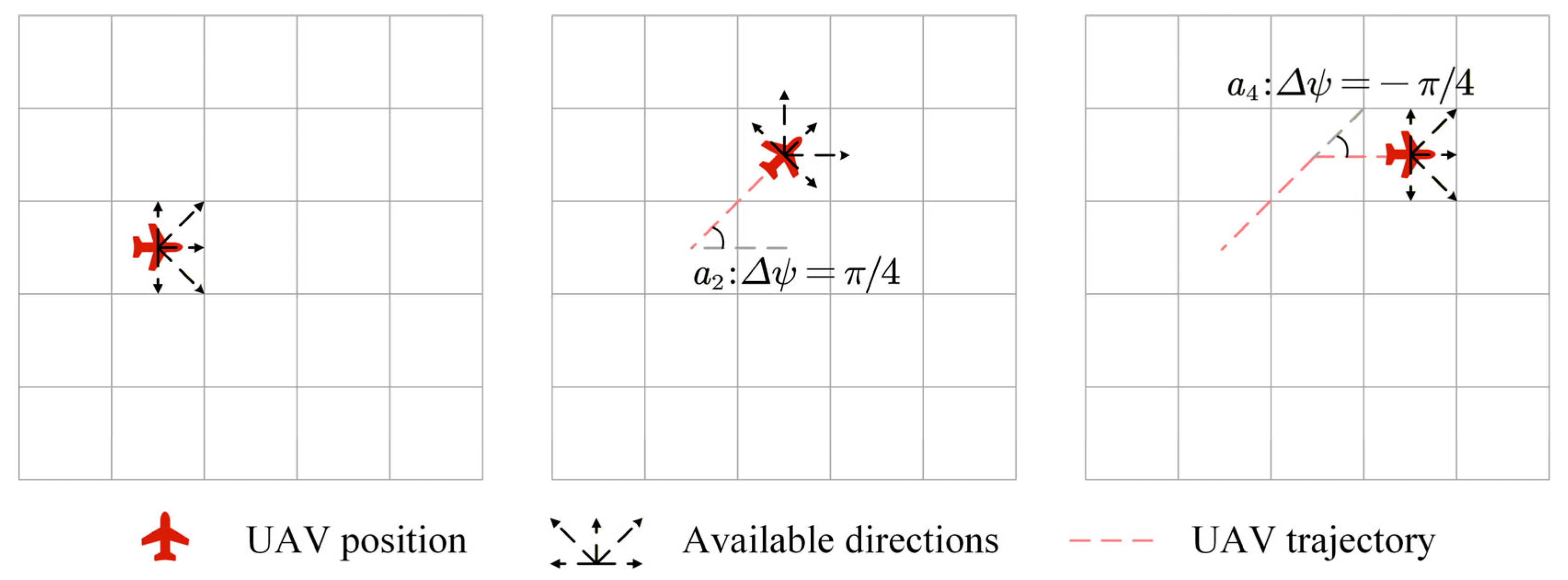
this set consists of five discrete actions: $a_1$: Maintain current heading and move forward one grid step. $a_2$: Turn left by $\pi /4$ and move forward one grid step. $a_3$: Turn left by $\pi /2$ and move forward one grid step. $a_4$: Turn right by $\pi /4$ and move forward one grid step. $a_5$: Turn right by $\pi /2$ and move forward one grid step. This kinematic model is illustrated in Figure 3.

3.3. Fusion Reward Shaping

Potential-based reward shaping is a technique that transforms prior knowledge into reward signals to alleviate the sparse reward problem and enhance exploration efficiency in reinforcement learning. This method achieves such shaping by defining a potential field, which provides additional intermediate reward signals on top of the sparse base rewards. Its mathematical form is:

$$R^{\prime }(s,\mathbf{a},s^{\prime })=R(s,\mathbf{a},s^{\prime })+\gamma \varphi (s^{\prime })-\varphi (s),$$

(22)

where $\varphi (\cdot )$ is the potential function, $\gamma$ is the discount factor, $R(s,\mathbf{a},s^{\prime })$ is the original reward, and $R^{\prime }(s,\mathbf{a},s^{\prime })$ is the reward after shaping. This method can theoretically guaranty the consistency of the optimal policy before and after reward shaping. For reinforcement learning, designing a reasonable potential field function is crucial for reward shaping.

Building on the above theory, in the dynamic target search scenario, the total reward is defined as:

$$R_{\mathrm{t}\mathrm{o}\mathrm{t}\mathrm{a}\mathrm{l}}=R_{\mathrm{b}\mathrm{a}\mathrm{s}\mathrm{e}}+R_{\mathrm{s}\mathrm{h}\mathrm{a}\mathrm{p}\mathrm{e}},$$

(23)

where $R_{\mathrm{b}\mathrm{a}\mathrm{s}\mathrm{e}}$ is the base reward, $R_{\mathrm{s}\mathrm{h}\mathrm{a}\mathrm{p}\mathrm{e}}$ is the shaping reward, and $R_{\mathrm{t}\mathrm{o}\mathrm{t}\mathrm{a}\mathrm{l}}$ is the final reward after shaping.

Specifically, building on the base environmental reward, this paper introduces three types of potential field functions: a Probability Edge Potential Field (${\varphi }^{\mathrm{e}\mathrm{d}\mathrm{g}\mathrm{e}}$), a Maximum Probability Potential Field (${\varphi }^{\mathrm{p}\mathrm{m}\mathrm{a}\mathrm{x}}$), and a Coverage Probability Sum Potential Field (${\varphi }^{\mathrm{p}\mathrm{c}\mathrm{o}\mathrm{v}}$). We also introduce an Adaptive Fusion Weight Mechanism to dynamically adjust their fusion weights. This mechanism allows the system to automatically identify and prioritize the most effective potential functions during training, thereby enhancing both learning efficiency and final policy quality.

The shaping reward is defined as:

$$R_{\mathrm{s}\mathrm{h}\mathrm{a}\mathrm{p}\mathrm{e}}={\sum }_{f\in \mathrm{e}\mathrm{d}\mathrm{g}\mathrm{e},\mathrm{p}\mathrm{m}\mathrm{a}\mathrm{x},\mathrm{p}\mathrm{c}\mathrm{o}\mathrm{v}}{\omega }_f\left[{\gamma \varphi }^f\left(s_{t+1}\right)-{\varphi }^f\left(s_t\right)\right],$$

(24)

where ${\omega }_f$ denotes the adaptive weight of potential function $f$.

In the following, we will elaborate on the base reward, the potential field functions, and the adaptive fusion weight mechanism in detail.

3.3.1. Base Reward

The base reward $R_{\mathrm{b}\mathrm{a}\mathrm{s}\mathrm{e}}^t$, is composed of two components, as defined in the following equation:

$$R_{\mathrm{b}\mathrm{a}\mathrm{s}\mathrm{e}}^t=R_{\mathrm{f}\mathrm{i}\mathrm{n}\mathrm{d}}^t+R_{\mathrm{p}\mathrm{r}\mathrm{i}\mathrm{o}\mathrm{r}}^t,$$

(25)

where the first component is a discovery reward $R_{\mathrm{f}\mathrm{i}\mathrm{n}\mathrm{d}}^t$, which incentivizes agents to find new targets. It provides a reward of +50 upon the discovery of a new target at timestep $t$, and 0 otherwise, and can be expressed as follows:

$$R_{\mathrm{f}\mathrm{i}\mathrm{n}\mathrm{d}}^t=\left\{\begin{array}{cc}50& \mathrm{i}\mathrm{f}\mathrm{f}\mathrm{i}\mathrm{n}\mathrm{d}=1\\ 0& \mathrm{o}\mathrm{t}\mathrm{h}\mathrm{e}\mathrm{r}\mathrm{w}\mathrm{i}\mathrm{s}\mathrm{e}\end{array}\right..$$

(26)

The second component is a prior probability reward $R_{\mathrm{p}\mathrm{r}\mathrm{i}\mathrm{o}\mathrm{r}}^t$, designed to encourage the exploration of high-probability areas. For visiting a grid cell ${\mathbf{q}}^{\mathrm{u}\mathrm{a}\mathrm{v}}(t)$, the agent receives a reward equal to 20 times the cell’s prior probability $p_{\mathrm{p}\mathrm{r}\mathrm{i}\mathrm{o}\mathrm{r}}(\mathbf{g})$, and can be expressed as follows:

$$R_{\mathrm{p}\mathrm{r}\mathrm{i}\mathrm{o}\mathrm{r}}^t=20\cdot p_{\mathrm{p}\mathrm{r}\mathrm{i}\mathrm{o}\mathrm{r}}({\mathbf{q}}^{\mathrm{u}\mathrm{a}\mathrm{v}}(t)).$$

(27)

The base reward $R_{\mathrm{b}\mathrm{a}\mathrm{s}\mathrm{e}}^t$ encourages the agent to explore high-probability areas to find more targets, but the reward signal is relatively sparse due to the limited probability distribution.

3.3.2. Multiple Potential Fields

To realize multi-potential field fusion reward shaping mechanism, this paper proposes three complementary potential field functions from both local and global perspectives: Probability Edge Potential Field ${\varphi }^{\mathrm{e}\mathrm{d}\mathrm{g}\mathrm{e}}$, Maximum Probability Potential Field ${\varphi }^{\mathrm{p}\mathrm{m}\mathrm{a}\mathrm{x}}$, and Coverage Probability Sum Potential Field ${\varphi }^{\mathrm{p}\mathrm{c}\mathrm{o}\mathrm{v}}$:

(1)

Probability Edge Potential Field ${\varphi }^{\mathrm{e}\mathrm{d}\mathrm{g}\mathrm{e}}$

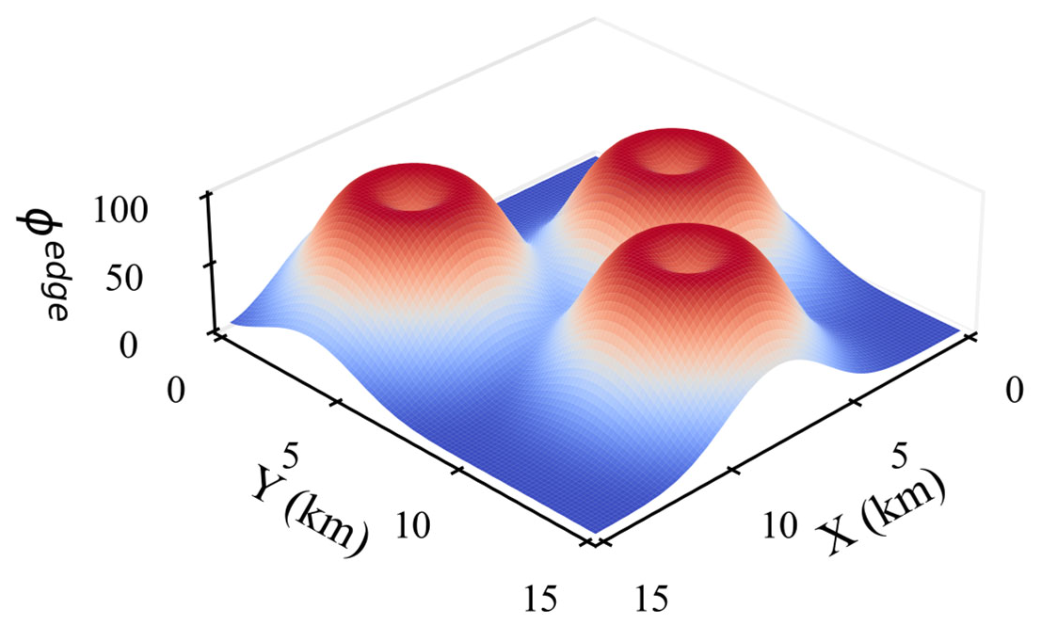
This potential field is defined from the perspective of local prior information. It is designed to guide agents toward the edge regions of the target probability distribution. In this way, agents obtain higher potential energy when approaching the probability boundary, thereby encouraging exploration around uncertain areas and improving search efficiency. As shown in Figure 4.

The potential field ${\varphi }^{\mathrm{e}\mathrm{d}\mathrm{g}\mathrm{e}}$ is defined as follows. The position of the $i$-th agent is:

$${\mathbf{q}}_i^{\mathrm{u}\mathrm{a}\mathrm{v}}=\left(x_i,y_i\right),i\in 1,\dots ,N_a.$$

(28)

The number of targets is $N_T$, and the probability area position of the $j$-th target is:

$${\mathcal{G}}_j=\{{\mathbf{g}}_{j,1},{\mathbf{g}}_{j,2},\dots ,{\mathbf{g}}_{j,M_j}\},j\in \{1,\dots ,N_T\},$$

(29)

where $M_j$ is the number of all possible positions of target $j$, and the set of probability values corresponding to each position is:

$${\mathcal{P}}_j=\{p({\mathbf{g}}_{j,1}),p({\mathbf{g}}_{j,2}),\dots ,p({\mathbf{g}}_{j,M_j})\}.$$

(30)

The minimum Euclidean distance from the $i$-th agent to the edge of the target probability area is defined as:

$$d_i^{\mathrm{e}\mathrm{d}\mathrm{g}\mathrm{e}}=\underset{1⩽j⩽N_T}{\mathrm{m}\mathrm{i}\mathrm{n}}\underset{1⩽k⩽M_j}{\mathrm{m}\mathrm{i}\mathrm{n}}\parallel {\mathbf{q}}_i^{\mathrm{u}\mathrm{a}\mathrm{v}}-{\mathbf{g}}_{j,k}\parallel .$$

(31)

Then the probability edge potential energy of the $i$-th agent is:

$${\varphi }_i^{\mathrm{e}\mathrm{d}\mathrm{g}\mathrm{e}}={\displaystyle \frac{C_0}{d_i^{\mathrm{e}\mathrm{d}\mathrm{g}\mathrm{e}}+1}},$$

(32)

where $C_0$ is the scale factor, which is used to control the range of the potential field value.

The global probability edge potential energy takes the average value of the potential energy of all agents and is processed by the Sigmoid fuzzy function, and can be expressed as follows:

$${\varphi }^{\mathrm{e}\mathrm{d}\mathrm{g}\mathrm{e}}(s)=\sigma \left({\displaystyle \frac{1}{N_a}}{\sum }_{i=1}^{N_a}{\varphi }_i^{\mathrm{e}\mathrm{d}\mathrm{g}\mathrm{e}}\right),$$

(33)

where

$$\sigma (x)={\displaystyle \frac{1}{1+e^{-a_{\sigma }(x-c_{\sigma })}}},$$

(34)

$\sigma$ is a Sigmoid-like fuzzy function, with parameter $a_{\sigma }$ controlling the steepness of the curve and $c_{\sigma }$ determining its center point. According to the definition, higher ${\varphi }^{\mathrm{e}\mathrm{d}\mathrm{g}\mathrm{e}}$ potential values correspond to the edges of the probability region, whereas positions farther from the edges exhibit lower potential values.

(2)

Maximum Probability Potential Field ${\varphi }^{\mathrm{p}\mathrm{m}\mathrm{a}\mathrm{x}}$

This potential field is constructed from the perspective of global optimal prediction.

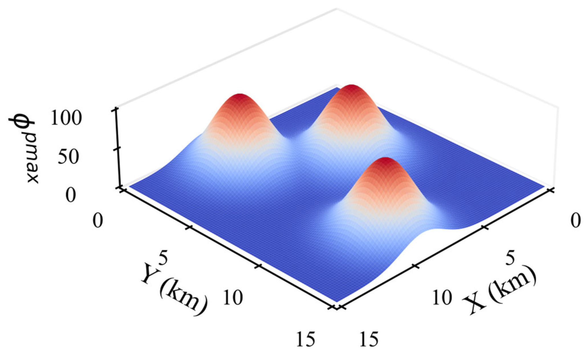
It is designed to guide agents toward the local maximum of the probability distribution. Positions closer to the maximum probability values yield higher potential energy, directing agents to the most likely target locations and thus accelerating target detection. As shown in Figure 5.

The potential field ${\varphi }^{\mathrm{p}\mathrm{m}\mathrm{a}\mathrm{x}}$ is defined as follows. The position of maximum probability for target $j$ is:

$${\mathbf{g}}_j^{\mathrm{m}\mathrm{a}\mathrm{x}}={\mathbf{g}}_{j,k_j^{\ast }},k_j^{\ast }=\mathrm{a}\mathrm{r}\mathrm{g}\underset{1⩽k⩽M_j}{\mathrm{m}\mathrm{a}\mathrm{x}}p({\mathbf{g}}_{j,k}).$$

(35)

The minimum distance from the $i$-th agent to all the maximum probability points is:

$$d_i^{\mathrm{p}\mathrm{m}\mathrm{a}\mathrm{x}}=\underset{1⩽j⩽N_T}{\mathrm{m}\mathrm{i}\mathrm{n}}\parallel {\mathbf{q}}_i^{\mathrm{u}\mathrm{a}\mathrm{v}}-{\mathbf{g}}_j^{\mathrm{m}\mathrm{a}\mathrm{x}}\parallel .$$

(36)

The local maximum probability potential energy of the $i$-th agent is:

$${\varphi }_i^{\mathrm{p}\mathrm{m}\mathrm{a}\mathrm{x}}={\displaystyle \frac{C_0}{d_i^{\mathrm{p}\mathrm{m}\mathrm{a}\mathrm{x}}+1}}.$$

(37)

Finally, the local maximum probability potential energy of all agents is first averaged to obtain a collective measure, and then this value is processed through a Sigmoid-like fuzzy mapping function to produce the global potential energy.

$${\varphi }^{\mathrm{p}\mathrm{m}\mathrm{a}\mathrm{x}}(s)=\sigma \left({\displaystyle \frac{1}{N_a}}{\sum }_{i=1}^{N_a}{\varphi }_i^{\mathrm{p}\mathrm{m}\mathrm{a}\mathrm{x}}\right).$$

(38)

According to the definition, positions closer to the maximum probability point of each target have higher ${\varphi }^{\mathrm{p}\mathrm{m}\mathrm{a}\mathrm{x}}$ potential values, while positions farther away exhibit lower values.

(3)

Coverage Probability Sum Potential Field ${\varphi }^{\mathrm{p}\mathrm{c}\mathrm{o}\mathrm{v}}$

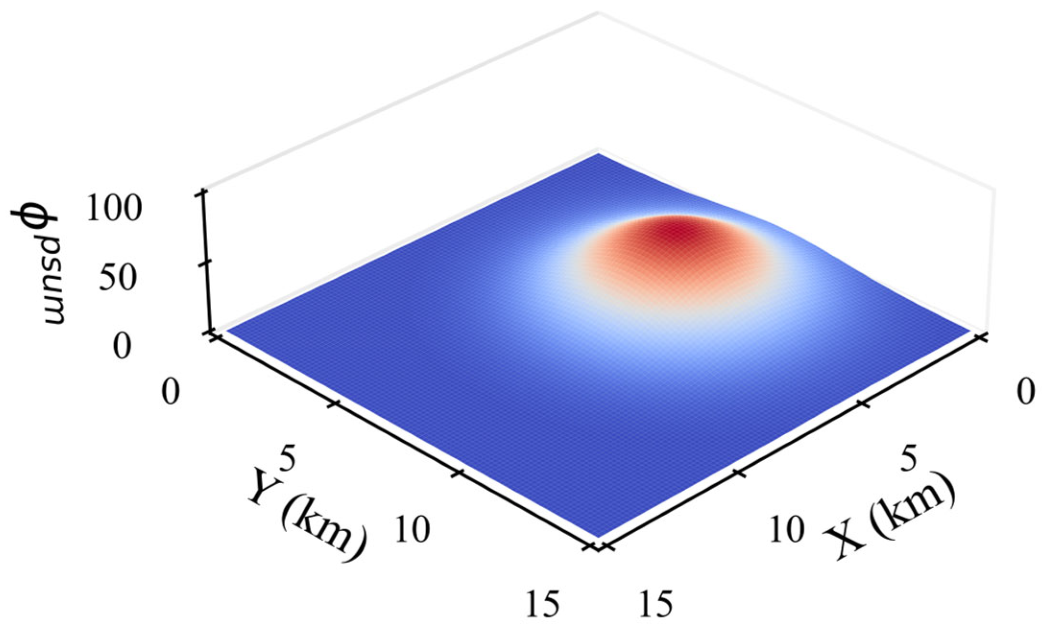
This potential field is proposed from the perspective of swarm-level coordination. It is designed to guide agents toward regions with the highest global coverage probability. Positions with larger cumulative probabilities correspond to higher potential energy, as shown in Figure 6.

The potential field ${\varphi }^{\mathrm{p}\mathrm{c}\mathrm{o}\mathrm{v}}$ is defined as follows. First, the sum of the existence probability of all targets at each grid position is calculated. This distribution is defined as the global coverage probability distribution, and can be expressed as follows:

$$C(\mathbf{g})={\sum }_{j=1}^{N_T}{\sum }_{k=1}^{M_j}p({\mathbf{g}}_{j,k})\cdot \mathbb{I}(\mathbf{g}={\mathbf{g}}_{j,k}),$$

(39)

where $\mathbb{I}\left(\cdot \right)$ is the indicator function.

From this distribution, we identify the grid position with the maximum coverage probability:

$${\mathbf{g}}^{\mathrm{c}\mathrm{o}\mathrm{v}\_\mathrm{m}\mathrm{a}\mathrm{x}}=\mathrm{a}\mathrm{r}\mathrm{g}\underset{\mathbf{g}\in \mathcal{M}}{\mathrm{m}\mathrm{a}\mathrm{x}}C(\mathbf{g}).$$

(40)

The distance from agent $i$ to this maximum coverage position is:

$$d_i^{\mathrm{p}\mathrm{c}\mathrm{o}\mathrm{v}}=\parallel {\mathbf{q}}_i^{\mathrm{u}\mathrm{a}\mathrm{v}}-{\mathbf{g}}^{\mathrm{c}\mathrm{o}\mathrm{v}\_\mathrm{m}\mathrm{a}\mathrm{x}}\parallel .$$

(41)

The total potential energy of its local coverage probability is:

$${\varphi }_i^{\mathrm{p}\mathrm{c}\mathrm{o}\mathrm{v}}={\displaystyle \frac{C_0}{d_i^{\mathrm{p}\mathrm{c}\mathrm{o}\mathrm{v}}+1}}.$$

(42)

The global coverage probability sum potential field function based on fuzzy logic is:

$${\varphi }^{\mathrm{p}\mathrm{c}\mathrm{o}\mathrm{v}}(s)=\sigma \left({\displaystyle \frac{1}{N_a}}{\sum }_{i=1}^{N_a}{\varphi }_i^{\mathrm{p}\mathrm{c}\mathrm{o}\mathrm{v}}\right).$$

(43)

According to the definition, positions closer to the points with higher cumulative coverage probability have larger ${\varphi }^{\mathrm{p}\mathrm{c}\mathrm{o}\mathrm{v}}$ potential values.

3.3.3. Adaptive Fusion Weight Mechanism

To adaptively fuse the above potential fields, this paper designs an adaptive fusion weight mechanism based on the correlation between advantage values and potential field values. In this way, multiple potential fields are combined according to their contribution to the advantage, forming a weighted shaping reward. The shaping reward is calculated as:

$$R_{\mathrm{s}\mathrm{h}\mathrm{a}\mathrm{p}\mathrm{e}}^t={\sum }_{f=1}^{N_f}{\mathsf{\omega }}_f\left(\gamma {\varphi }^f(s_{t+1})-{\varphi }^f(s_t)\right),$$

(44)

where $N_f$ is the number of potential fields, and ${\varphi }^f$ is the f-th potential field. In this mechanism, the fusion weights of each potential field function are modeled as random variables that obey the Dirichlet distribution, and satisfy the following constraints [44]:

$$\mathsf{\omega }\in \left\{\mathsf{\omega }\in {\mathbb{R}}^{N_f}:{\sum }_{f=1}^{N_f}{\omega }_f=1,{\omega }_f\ge 0\right\},$$

(45)

where $N_f$ represents the number of potential field functions. By utilizing Bayesian updating theory, the parameter vector of the Dirichlet distribution is dynamically adjusted to achieve adaptive optimization of the weight distribution of each potential field function. The parameter vector can be expressed as follows:

$$\mathsf{\alpha }=({\alpha }_1,{\alpha }_2,\cdots ,{\alpha }_{N_f}).$$

(46)

The update is based on the Pearson correlation coefficient between each potential energy value and the advantage value, so that the potential field function with a strong positive correlation with the advantage value obtains a higher weight, so as to play a greater role in the reward shaping process. This method is specifically for policy optimization reinforcement learning methods.

During a warm-up phase, agents are trained using only the base reward, $R_{\mathrm{b}\mathrm{a}\mathrm{s}\mathrm{e}}^t$. This promotes the initial convergence of the value network, which in turn improves the credibility of the advantage function estimates.

Following the warm-up, the weight adjustment phase begins. In this phase, agents interact with the environment to collect trajectory data during each episode. For each timestep t in a trajectory, the following data tuple is recorded:

$$\tau ={\left\{s_t,{\mathbf{a}}_t,A(s_t,{\mathbf{a}}_t),{\left[{\varphi }^f(s_t)\right]}_{f=1}^{N_f}\right\}}_{t=1}^L,$$

(47)

where $s_t$ represents the global state, which in this implementation is constructed by aggregating all agents’ local observations. ${\mathbf{a}}_t$ represents the joint action, $A(s_t,{\mathbf{a}}_t)$ is the advantage value, ${\varphi }^i\left(s_t\right)$ represents the potential energy value of the $i$-th potential field function under the state $s_t$, and $L$ is the length of the trajectory.

For each potential field function ${\varphi }^i$, extract the advantage value and potential energy value data pair ${\left\{A_t,{\varphi }_t^f\right\}}_{t=1}^L$. And perform the following steps.

Calculate the mean value of the potential energy is calculated as:

$${\mu }_{{\varphi }^f}={\displaystyle \frac{1}{L}}{\sum }_{t=1}^L{\varphi }_t^f.$$

(48)

Calculate the mean of the odds ratio is calculated as:

$${\mu }_A={\displaystyle \frac{1}{L}}{\sum }_{t=1}^L{A}_t.$$

(49)

Calculate the Pearson correlation coefficient between the potential energy value and the advantage value is calculated as:

$${\rho }_f={\displaystyle \frac{\sum _{t=1}^L({\varphi }_t^f-{\mu }_{{\varphi }^f})(A_t-{\mu }_A)}{\sqrt{\sum _{t=1}^L({\varphi }_t^f-{\mu }_{{\varphi }^f}{)}^2}\sqrt{\sum _{t=1}^L(A_t-{\mu }_A{)}^2}}}.$$

(50)

The correlation coefficients are truncated and normalized, and the process can be expressed as follows:

$${\rho }_f\leftarrow \mathrm{m}\mathrm{a}\mathrm{x}({\rho }_f,0),{\rho }_f\leftarrow {\rho }_f/{\sum }_{f^{\prime }=1}^{N_f}{\rho }_{f^{\prime }}.$$

(51)

Update the Dirichlet distribution parameters using the normalized coefficients, and can be expressed as follows:

$${\alpha }_f^{\mathrm{n}\mathrm{e}\mathrm{w}}={\alpha }_f^{\mathrm{o}\mathrm{l}\mathrm{d}}+\eta \cdot {\rho }_f,$$

(52)

where $\eta$ is the learning rate for updating the Dirichlet parameters.

After updating the parameters, the mean of the Dirichlet distribution is used as the new weight of the potential field function, and the calculation formula is:

$${\omega }_f={\alpha }_f/{\sum }_{f^{\prime }=1}^{N_f}{\alpha }_{f^{\prime }}.$$

(53)

In summary, the proposed mechanism enables adaptive adjustment of fusion weights, ensuring a balanced contribution of different potential fields to the overall shaping reward. The Adaptive Fusion Weight Mechanism is outlined in Algorithm 1.

Algorithm 1. Adaptive Fusion Weight Mechanism.

1: Input: Number of potential fields $N_f$, learning rate $\eta$, trajectory length $L$

2: Initialize: Dirichlet parameters $\mathsf{\alpha }=\left({\alpha }_1,{\alpha }_2,\cdots ,{\alpha }_{N_f}\right)$ uniformly

3: Warm-up Phase:

Agents are trained using only base reward $R_{\mathrm{base}}^t$ to stabilize value estimation

4: Weight Adjustment Phase:

5: for each episode do

6:    Collect trajectory $\tau =\{s_t,{\mathbf{a}}_t,A_t,{\left[{\varphi }_t^f\right]}_{f=1}^{N_f}{\}}_{t=1}^L$

7:    for each potential field $f=1$ to $N_f$ do

8:    Compute mean potential energy: ${\mu }_{{\varphi }^f}={\displaystyle \frac{1}{L}}{\sum }_{t=1}^L{\varphi }_t^f$

9:    Compute mean advantage: ${\mu }_A={\displaystyle \frac{1}{L}}{\sum }_{t=1}^L{A}_t$

10:     Compute Pearson correlation coefficient:

${\rho }_f={\displaystyle \frac{{\sum }_{t=1}^L\left({\varphi }_t^f-{\mu }_{{\varphi }^f}\right)\left(A_t-{\mu }_A\right)}{\sqrt{{\sum }_{t=1}^L{\left({\varphi }_t^f-{\mu }_{{\varphi }^f}\right)}^2}\sqrt{{\sum }_{t=1}^L{\left(A_t-{\mu }_A\right)}^2}}}$

11:    Truncate and normalize: ${\rho }_f\leftarrow \max \left({\rho }_f,0\right)$

12:  end for

13:  Normalize correlations: ${\rho }_f\leftarrow {\rho }_f/{\sum }_{f^{\prime }=1}^{N_f}{\rho }_{f^{\prime }}$

14:  for each potential field $f=1$ to $N_f$ do

15:    Update Dirichlet parameter: ${\alpha }_f\leftarrow {\alpha }_f+\eta \cdot {\rho }_f$

16:  end for

17:  for each potential field $f=1$ to $N_f$ do

18:    Compute new weight: ${\omega }_f={\alpha }_f/{\sum }_{f^{\prime }=1}^{N_f}{\alpha }_{f^{\prime }}$

19:  end for

20: end for

3.4. MPRS-MAPPO Algorithm

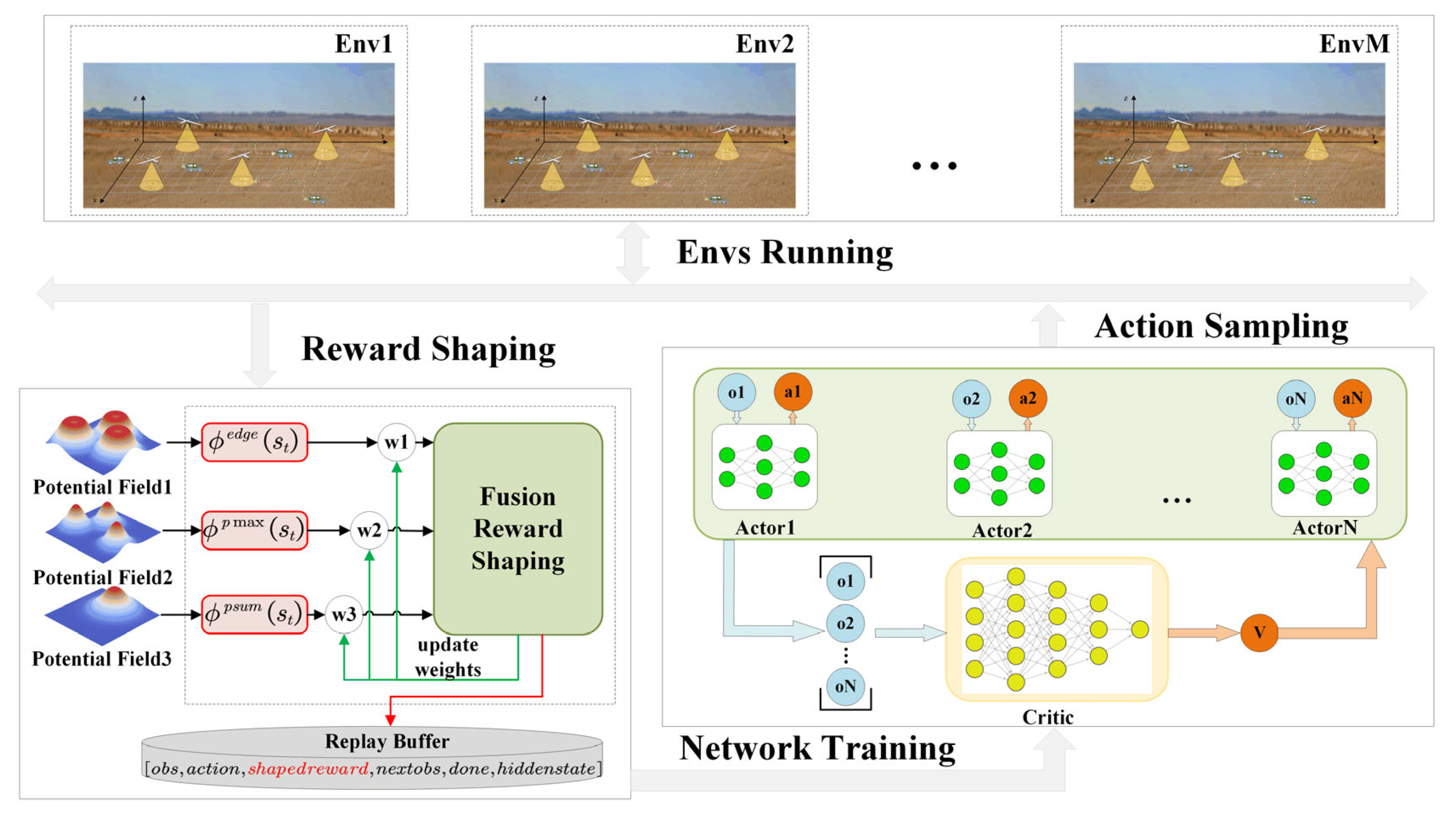
Based on the above potential fields and fusion mechanism, we propose the MPRS-MAPPO algorithm. The algorithm introduces a multi-potential field fusion reward shaping mechanism on the basis of the standard MAPPO framework [26] and adopts a centralized training and decentralized execution (CTDE) architecture. During training, each agent collects experience tuples consisting of states, actions, and shaped rewards, which are stored in a shared replay buffer. During centralized training, the global state is used by the value network and for reward shaping to stabilize learning. During decentralized execution, each UAV makes decisions based only on its local observation. The fusion weights of the potential fields are updated adaptively based on their correlation with advantage values, ensuring that more informative potentials have a stronger influence on learning. This allows agents to efficiently explore the environment while maintaining coordinated behavior.

Its core innovation lies in using the multi-potential field fusion module to correct the original environment reward in real time and guide the agent to learn the cooperative policy. Meanwhile, the proposed mechanism is fully compatible with the existing MAPPO algorithm based on policy optimization. The framework of the algorithm is shown in Figure 7.

The key steps of the centralized training of the algorithm are as follows:

(1)

Action And Environment Sampling

The MPRS-MAPPO framework inherits the policy optimization approach of MAPPO, where each agent $i$ has an independent policy network ${\pi }_{{\theta }^i}$ and a shared value network $v_{{\omega }^i}$. At each timestep $t$, multiple parallel environments provide a set of local observations ${\left\{o_t^i\right\}}_{i=1}^{N_a}$. Each agent then samples an action $a_t^i$ from its respective policy network, forming action set ${\left\{a_t^i\right\}}_{i=1}^{N_a}$. After executing this joint action, the environment returns the next observations and the base reward $R_{\mathrm{b}\mathrm{a}\mathrm{s}\mathrm{e}}^t$.

(2)

Reward Shaping

The multi-potential field fusion shaping module shapes the original reward to obtain the shaping reward $R_{\mathrm{s}\mathrm{h}\mathrm{a}\mathrm{p}\mathrm{e}}^t$, where the fusion weights are computed using Algorithm 1:

$$\begin{gathered} R_{\mathrm{s}\mathrm{h}\mathrm{a}\mathrm{p}\mathrm{e}}^t=[{\omega }_{\mathrm{e}\mathrm{d}\mathrm{g}\mathrm{e}}\left({\gamma \varphi }^{\mathrm{e}\mathrm{d}\mathrm{g}\mathrm{e}}\left(s_{t+1}\right)-{\varphi }^{\mathrm{e}\mathrm{d}\mathrm{g}\mathrm{e}}\left(s_t\right)\right)+{\omega }_{\mathrm{p}\mathrm{m}\mathrm{a}\mathrm{x}}(\gamma {\varphi }^{\mathrm{p}\mathrm{m}\mathrm{a}\mathrm{x}}(s_{t+1})- \\ {\varphi }^{\mathrm{p}\mathrm{m}\mathrm{a}\mathrm{x}}(s_t))+\left.{\omega }_{\mathrm{p}\mathrm{c}\mathrm{o}\mathrm{v}}\left({\gamma \varphi }^{\mathrm{p}\mathrm{c}\mathrm{o}\mathrm{v}}(s_{t+1})-{\varphi }^{\mathrm{p}\mathrm{c}\mathrm{o}\mathrm{v}}(s_t)\right)\right]. \end{gathered}$$

(54)

The final reward, $R_{\mathrm{t}\mathrm{o}\mathrm{t}\mathrm{a}\mathrm{l}}^t$ is the sum of the base reward $R_{\mathrm{b}\mathrm{a}\mathrm{s}\mathrm{e}}^t$ and the shaping reward $R_{\mathrm{s}\mathrm{h}\mathrm{a}\mathrm{p}\mathrm{e}}^t$. The experience data $\left(s_t,a_t,R_{total}^t,s_{t+1}\right)$ is stored in the experience replay buffer. Here, the potential field functions ${\varphi }^{\mathrm{e}\mathrm{d}\mathrm{g}\mathrm{e}}$, ${\varphi }^{\mathrm{p}\mathrm{m}\mathrm{a}\mathrm{x}}$, and ${\varphi }^{\mathrm{p}\mathrm{c}\mathrm{o}\mathrm{v}}$ are all computed from the global state to ensure that shaping reflects the cooperative search context.

In the reward shaping stage, the global state which aggregates all agents’ local observations is used to compute the potential field values. This allows the shaping module to consider the overall spatial distribution of UAVs and targets, thereby maintaining consistent cooperative guidance.

(3)

Value Network Update

The shared value network is updated by minimizing the following loss function, where the global state $s_t$ is used as input to estimate the overall expected return of the multi-UAV system:

$$L\left({\omega }^i\right)={\mathbb{E}}_{s_t}\left[{\left(v_{{\omega }^i}\left(s_t\right)-{\widehat{R}}_i^t\right)}^2\right],$$

(55)

where ${\widehat{R}}_i^t=\sum _{t^{\prime }=t}^{\mathrm{\infty }}{\gamma }^{t^{\prime }-t}{R}_{\mathrm{t}\mathrm{o}\mathrm{t}\mathrm{a}\mathrm{l}}^t$ is the cumulative discounted return.

During centralized training, the value network receives the global state $s_t$ as input, allowing it to estimate the overall expected return of the multi-agent system. This enables each agent’s policy to be optimized with respect to the joint environment dynamics.

(4)

Policy Network Update

Each agent’s policy network ${\pi }_{{\theta }^i}$ uses only its local observation $o_t^i$ to select actions, ensuring decentralized execution. However, during training, policy optimization is performed using advantage estimates derived from the global value function, thereby integrating centralized information into decentralized learning.

The objective function of policy update is:

$$L\left({\theta }^i\right)={\mathbb{E}}_{(s_t,a_t)}\left[\mathrm{m}\mathrm{i}\mathrm{n}\left(r_t({\theta }^i)A_{{\theta }^{i^{\prime }}}{(o}_t^i,a_t^i),\mathrm{c}\mathrm{l}\mathrm{i}\mathrm{p}(r_t{(\theta }^i),1-\epsilon ,1+\epsilon {)A}_{{\theta }^{i^{\prime }}}{o}_t^i,a_t^i)\right)\right],$$

(56)

where $r_t\left(\theta \right)={\displaystyle \frac{{\pi }_{\theta }\left(a_t|o_t^i\right)}{{\pi }_{{\theta }^{\prime }}\left(a_t|o_t^i\right)}}$ is the importance sampling ratio, $\mathrm{c}\mathrm{l}\mathrm{i}\mathrm{p}\left(\cdot \right)$ limits the policy update range, and $A_{{\theta }^{i^{\prime }}}$ is the generalized advantage estimation (GAE), which is calculated as follows:

$$A_{{\theta }^{i^{\prime }}}={\sum }_{l=0}^{\infty }(\gamma \lambda {)}^l{\delta }_{t+l}^i,{\delta }_t^i=R_{total}^t+\gamma v_{{\omega }^i}\left(s_{t+1}\right)-v_{{\omega }^i}\left(s_t\right),$$

(57)

where $\gamma$ is the reinforcement learning discount factor, $\lambda$ is the hyperparameter of GAE, and ${\delta }_t^i$ is the temporal difference (TD) error of agent $i$ at time $t$.

In the distributed execution phase of the algorithm, each agent relies on its own local observation $o_t^i$ and the converged policy network to make independent decisions, realizing complete decentralized control. As shown in the following:

$$a_t^i=arg\underset{a}{\mathrm{m}\mathrm{a}\mathrm{x}}{\pi }_{{\theta }^i}\left(a|o_t^i\right).$$

(58)

The key to this architecture is the design of three complementary potential functions (${\varphi }^{\mathrm{e}\mathrm{d}\mathrm{g}\mathrm{e}},{\varphi }^{\mathrm{p}\mathrm{m}\mathrm{a}\mathrm{x}},{\varphi }^{\mathrm{p}\mathrm{c}\mathrm{o}\mathrm{v}}$), each with a distinct focus. These are integrated via the Adaptive Fusion Weight Mechanism, which balances their respective contributions during training. The adaptive mechanism dynamically adjusts the fusion weights according to their correlation with the advantage values, ensuring that more informative potential fields have a stronger influence at each training stage. By assigning greater weight to functions that are more beneficial for learning, this method improves both training efficiency and the quality of the final converged policy. The complete MPRS-MAPPO algorithm is outlined in Algorithm 2.

Algorithm 2. MPRS-MAPPO.

1: Notations:

$\theta$: policy network parameters (actor)

$\omega$: value network parameters (critic)

$\mathsf{\alpha }$: Dirichlet distribution parameters (from Algorithm 1)

$D$: experience buffer

$W$: warm-up stage length, $T$: episode horizon, $K$: update iterations

${\eta }_{\theta }$,${\eta }_{\omega }$,${\eta }_{\alpha }$: learning rates

${\varphi }^f$: potential field functions $\{{\varphi }^{\mathrm{edge}},{\varphi }^{\mathrm{pmax}},{\varphi }^{\mathrm{pcov}}\}$

${\mathsf{\omega }}_f$: adaptive fusion weight of field $f$

$R_{\mathrm{base}},R_{\mathrm{shape}},R_{\mathrm{total}}$: base, shaping, and total rewards

2: Initialize: $\theta$, $\omega$, $\alpha$(uniform), $D=\mathrm{\varnothing }$, $episode=0$

3: while policy not converged do

4:    $episode\leftarrow episode+1$

5:    for t = 1 to$T$do

6:    Each agent $i$: sample $a_t^i\sim {\pi }_{{\theta }^i}(o_t^i)$

7:    ($s_{t+1}$, $R_{\mathrm{b}\mathrm{a}\mathrm{s}\mathrm{e}}$) ← $env.step\left({\mathbf{a}}_t\right)$

8:    if $episode$ ≤ $W$then                    $⊳$Warm-up

9:      $R_{\mathrm{t}\mathrm{o}\mathrm{t}\mathrm{a}\mathrm{l}}=R_{\mathrm{b}\mathrm{a}\mathrm{s}\mathrm{e}}$

10:     else                   $⊳$Fusion Reward Shaping

11:      $R_{\mathrm{s}\mathrm{h}\mathrm{a}\mathrm{p}\mathrm{e}}={\sum }_{f\in \mathrm{e}\mathrm{d}\mathrm{g}\mathrm{e},\mathrm{p}\mathrm{m}\mathrm{a}\mathrm{x},\mathrm{p}\mathrm{c}\mathrm{o}\mathrm{v}}{\omega }_f\left[{\gamma \varphi }^f\left(s_{t+1}\right)-{\varphi }^f\left(s_t\right)\right]$

12:      $R_{\mathrm{t}\mathrm{o}\mathrm{t}\mathrm{a}\mathrm{l}}=R_{\mathrm{b}\mathrm{a}\mathrm{s}\mathrm{e}}+R_{\mathrm{s}\mathrm{h}\mathrm{a}\mathrm{p}\mathrm{e}}$

13:    end if

14:    $D.add\left(s_t,{\mathbf{a}}_t,R_{\mathrm{t}\mathrm{o}\mathrm{t}\mathrm{a}\mathrm{l}},s_{t+1}\right)$

15:  end for

16:  if $episode$>$W$then              $⊳$Adaptive Fusion Weights

17:     Call Algorithm 1 to update ${\alpha }_f$and compute${\omega }_f$

18:  end if

19:  for $k$= 1 to $K$do               $⊳$Policy and Value Updates

20:     $\widehat{R}=\sum _{l=0}^{\mathrm{\infty }}{\gamma }^l{R}_{\mathrm{t}\mathrm{o}\mathrm{t}\mathrm{a}\mathrm{l}}^{t+l}$

21:     $\omega \leftarrow \omega -{\eta }_{\omega }{\nabla }_{\omega }\mathbb{E}\left[{\left(v_{\omega }\left(s_t\right)-\widehat{R}\right)}^2\right]$

22:     $A_t^{GAE}={\sum }_{l=0}^{\mathrm{\infty }}{\left(\gamma \lambda \right)}^l{\delta }_{t+l}$

23:     ${\theta }^i\leftarrow {\theta }^i+{\eta }_{\theta }{\nabla }_{{\theta }^i}\mathbb{E}[\mathrm{m}\mathrm{i}\mathrm{n}(r_t{A}_t^{GAE},\mathrm{c}\mathrm{l}\mathrm{i}\mathrm{p}(r_t,1\pm \epsilon )A_t^{GAE})]$

21:  end for

25: end while

4. Results and Discussion

To evaluate the performance of the proposed MPRS-MAPPO algorithm in multi-UAV cooperative search tasks, we designed representative scenarios in which multiple UAVs search for multiple dynamic targets. Systematic experiments were conducted using baseline algorithms and multiple evaluation metrics, and ablation studies were further performed to analyze the performance contributions of individual components. The experiments include both simulation tests and physical flight experiments. The experimental setup and results are presented as follows.

4.1. Experimental Environment and Parameter Settings

The experiments were conducted on a high-performance workstation (Intel i7-13700KF, 32 GB RAM, NVIDIA RTX 3060Ti), where a multi-UAV cooperative search simulation environment was built using PyTorch (version 2.3.0) and OpenAI Gym (version 0.20.0).

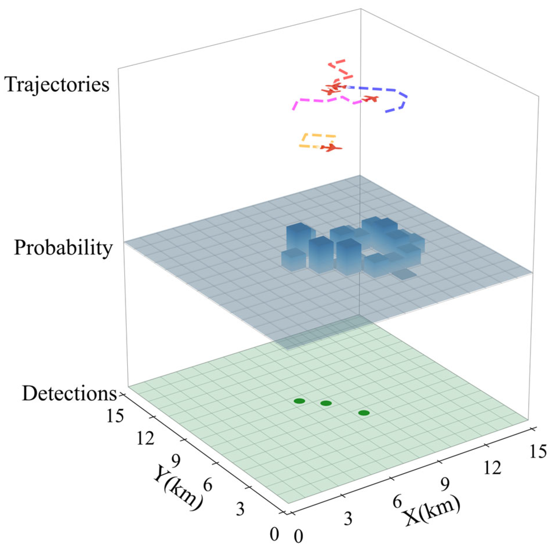
As shown in Figure 8, the schematic of the simulation environment is organized into three layers: the top layer displays the current positions and trajectories of the UAVs, the middle layer presents the probabilistic estimates of undiscovered target locations, and the bottom layer shows the positions of detected targets. This simulation environment integrates UAV agents, dynamic targets, and probability distributions derived from sensor observations.

The simulation area was defined as a 15 km × 15 km discrete grid (step size: 1 km). In the representative 4v6 scenario, four UAVs were initialized at random positions to search for six dynamic targets. Each UAV was modeled as a fixed-wing aircraft with a speed of 60 m/s, capable of performing forward, left-turn, and right-turn maneuvers. Collision avoidance was achieved by altitude separation (0.9–1.1 km). The onboard sensor had a coverage of 1 km × 1 km, a detection probability of 0.95, and a false alarm probability of 0.05. Targets moved randomly at approximately 20 m/s and could potentially leave the area.

The main experimental parameters for the UAV search task are summarized in

Table 2. Experimental parameter settings for UAV search task.

Parameter	Value
Area size	15 km × 15 km
Number of UAVs/Targets	2, 4, 6/3, 6, 9
UAV speed	60 m/s
Target speed	20 m/s
Detection probability	0.95
False alarm probability	0.05
Episode length	200
Actor/Critic learning rate	1 × 10−5/2 × 10−5
Discount factor $\gamma$	0.99
GAE $\lambda$	0.95
PPO clipping parameter	0.2
Warm-up rollouts	40

. The environment size, UAV/target numbers, and their speeds define task dynamics, while detection and false alarm probabilities reflect sensing reliability. For training, episode length, learning rates, discount factor, GAE parameter, PPO clipping, and warm-up rollouts are specified.

4.2. Algorithm Effectiveness Analysis

To verify the effectiveness of the proposed algorithm, detailed analyses were first conducted under the standard experimental configuration of 4 UAVs and 6 targets (4v6). Experiments were conducted with 10 different random seeds. The evaluation metrics include the convergence trends of return and target detection rate, the dynamic variations in the three potential field weights, and the UAV search trajectories after training.

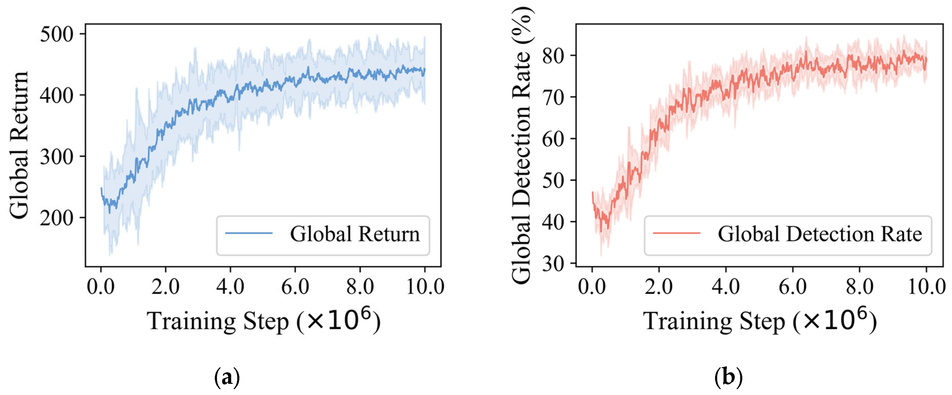
During training, the global return and target detection rate of MPRS-MAPPO both exhibited stable convergence, as shown in Figure 9. Specifically, the return increased from 232.47 to 451.43, while the target detection rate rose from 41.52% to 78.89%, demonstrating the algorithm’s strong optimization capability and convergence properties.

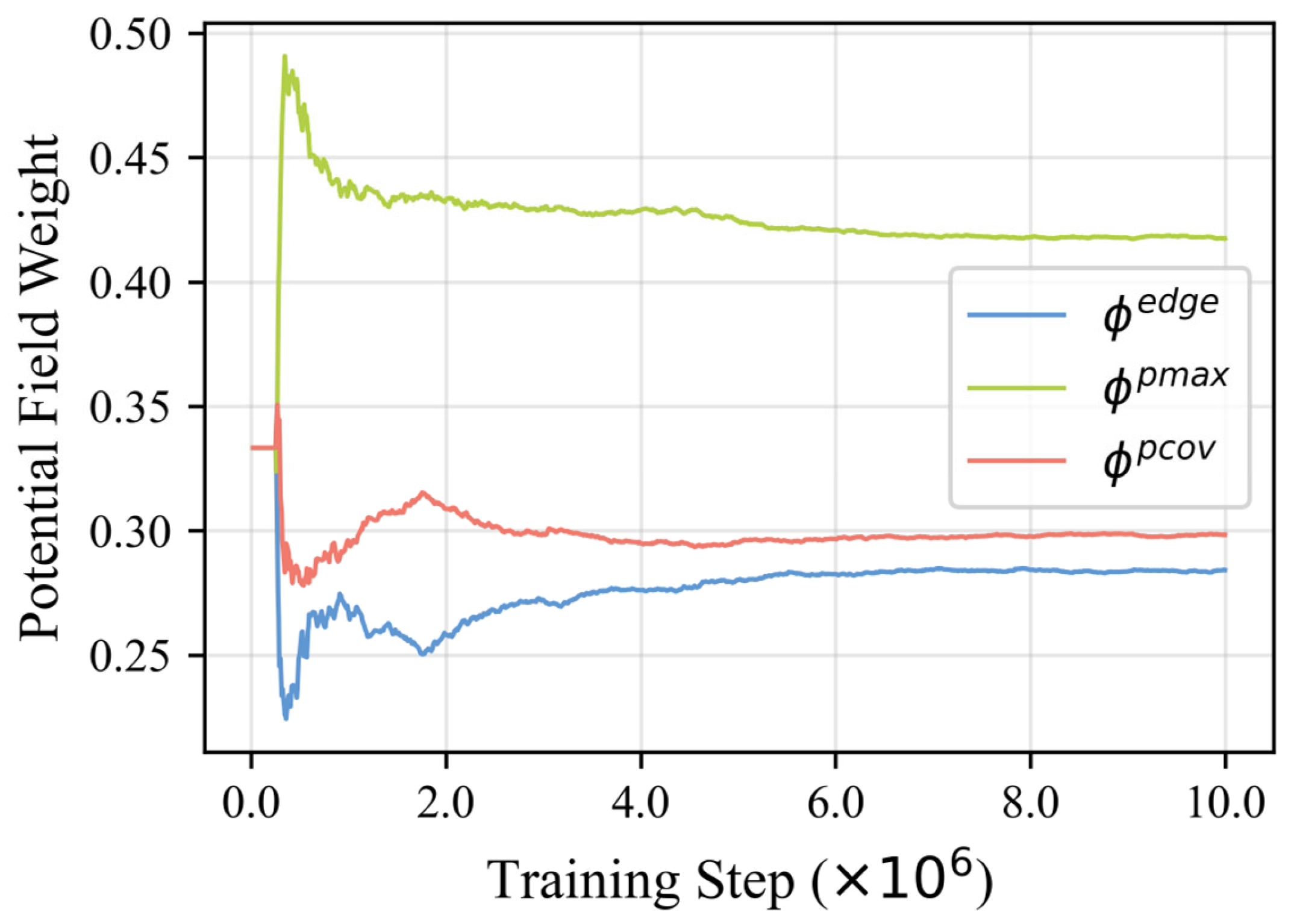
As illustrated in Figure 10, during the warm-up phase, the weights of the three potential field functions were evenly initialized at 33.33%. After the warm-up, the weight of the Maximum Probability Potential Field ${\varphi }^{\mathrm{p}\mathrm{m}\mathrm{a}\mathrm{x}}$ rapidly increased to 48.36%, then decreased and stabilized at 42.14%, showing a “rise-then-fall” trend. In contrast, the weights of the Probability Edge Potential Field ${\varphi }^{\mathrm{e}\mathrm{d}\mathrm{g}\mathrm{e}}$ and the Coverage Probability Sum Potential Field ${\varphi }^{\mathrm{p}\mathrm{c}\mathrm{o}\mathrm{v}}$ initially dropped to 23.86% and 27.61%, respectively, and later gradually increased, stabilizing at 27.38% and 29.47%. This dynamic adaptation validates the algorithm’s capability for multi-potential field fusion.

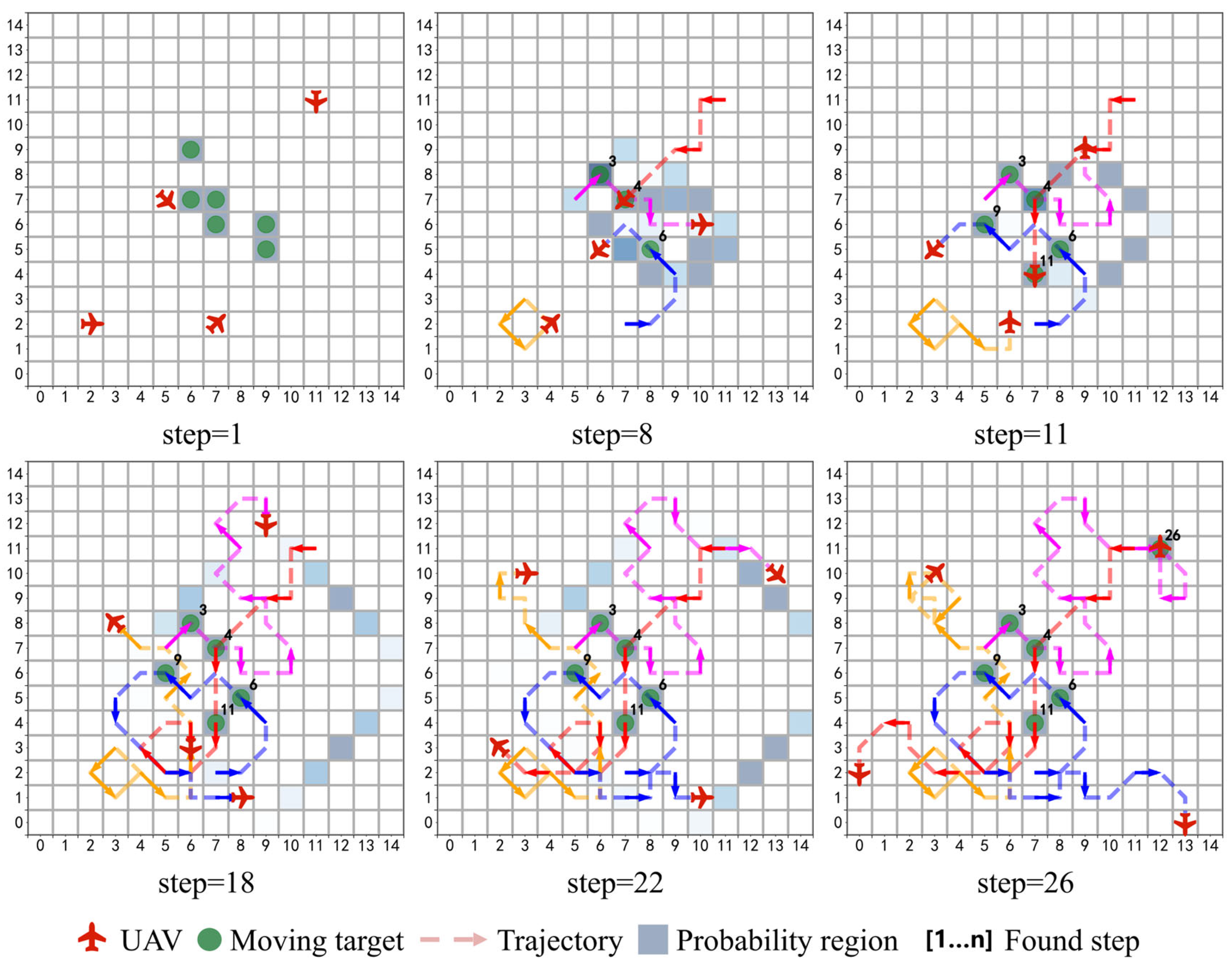
Figure 11 illustrates the execution process of the UAVs. Red aircraft represent the agents, and green dots denote the true target positions (visible only initially or upon discovery).

At the beginning, targets were randomly distributed. By step 8, the UAVs had detected three targets and gradually converged toward high-probability areas; by step 11, two additional targets were detected; and by step 26, all targets were successfully located. The trajectories demonstrate that the UAVs progressively shifted from concentrated search to distributed coverage, thereby improving overall efficiency.

For clarity, the discovery time of each target is annotated at its upper right corner, while the movement directions of the UAVs are indicated along their respective trajectories.

In terms of real-time performance, the average decision-making time per step was approximately 0.015 s, indicating that the proposed method can meet real-time requirements in online multi-UAV cooperative search scenarios.

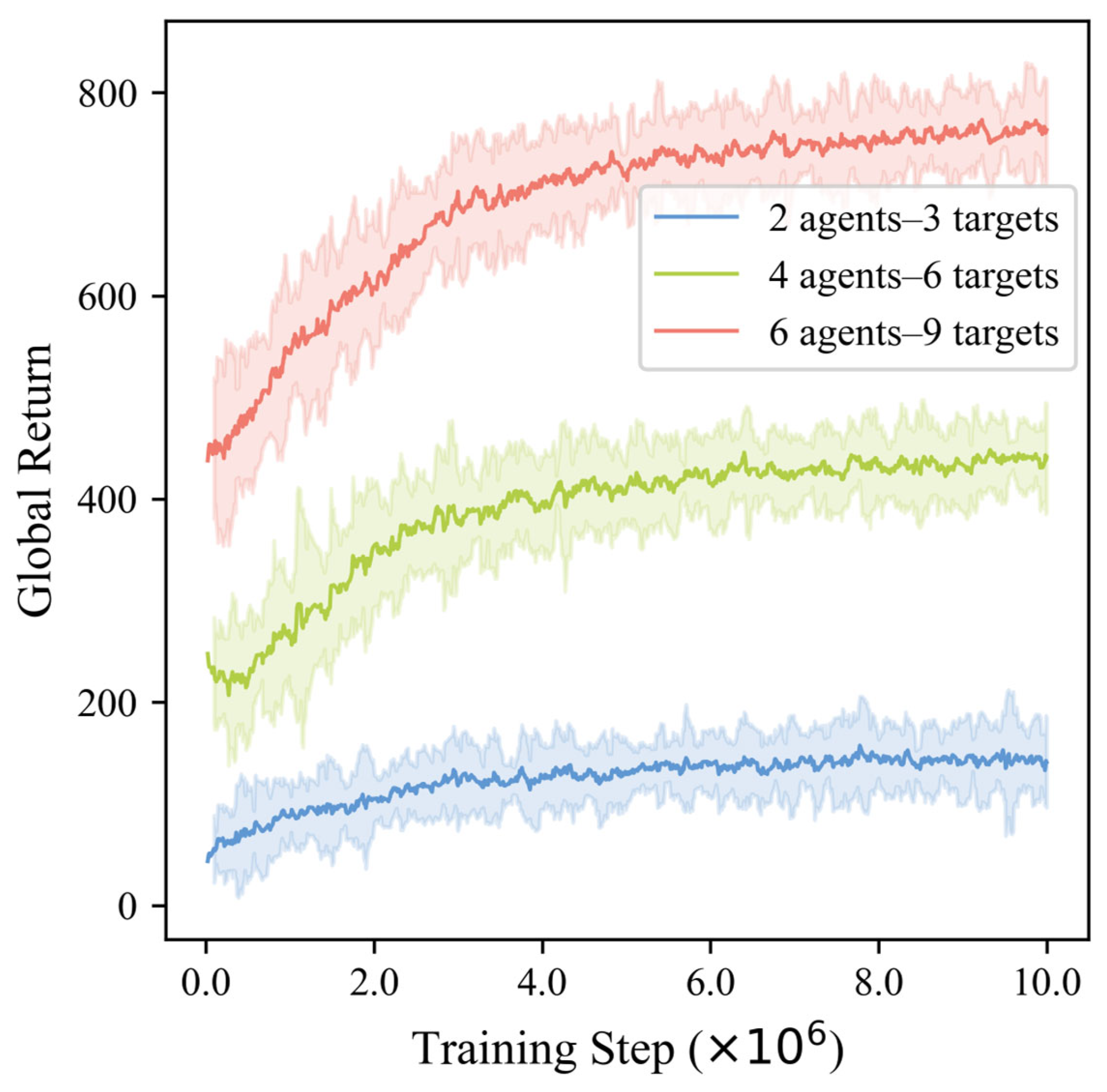
To further evaluate the robustness and scalability of the proposed algorithm, comparative experiments were conducted under different task scales, including 2 UAVs vs. 3 targets (2v3), 4 UAVs vs. 6 targets (4v6), and 6 UAVs vs. 9 targets (6v9). The 6v9 scenario involved a more complex case where several targets were initialized in close proximity. The convergence curves of global return under different task scales are shown in Figure 12. The results indicate that the algorithm achieved effective convergence across all configurations, with slightly slower convergence as task complexity increased. Since the number of targets differs among scenarios, the return curves are distributed at different height levels accordingly.

4.3. Comparison with Existing Methods

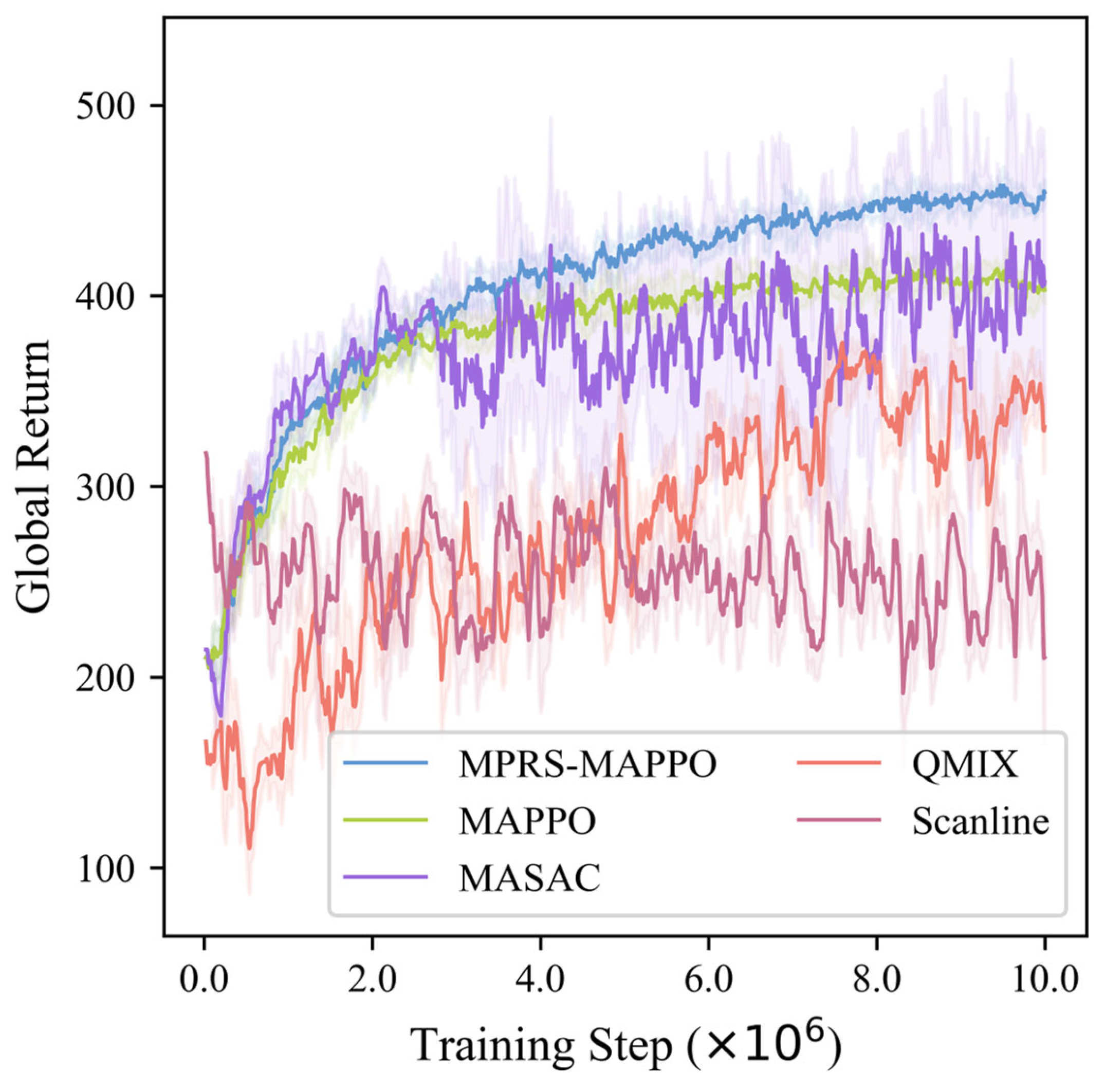
To comprehensively evaluate the overall performance of MPRS-MAPPO, four representative methods were selected as baselines: three multi-agent reinforcement learning algorithms, MAPPO, MASAC and QMIX, and a heuristic coverage-based search strategy, Scanline. The evaluation metrics included global return curve trends, converged return values, target detection rate, and the rolling standard deviation of the return curves.

MAPPO [26] is a multi-agent policy optimization algorithm that performs centralized training with decentralized execution and uses a clipped surrogate objective to stabilize policy updates. It effectively balances policy improvement and variance control, making it a widely adopted baseline in cooperative MARL tasks.

MASAC [37] is an off-policy, entropy-regularized algorithm that enhances the exploration and stability of multi-agent systems, particularly in environments with incomplete information.

QMIX [25] is a value-based multi-agent reinforcement learning algorithm that decomposes the joint action-value function into individual agent contributions while ensuring monotonicity.

Scanline [10] is a heuristic coverage-based search method that directs UAVs along pre-defined sweeping paths to maximize area coverage and target detection. Although simple and easy to implement, it lacks learning ability and adaptability in dynamic or partially observable environments.

As shown in Figure 13, MPRS-MAPPO outperformed the other algorithms in terms of both convergence speed and stability. While MAPPO and QMIX improved policy performance to some extent, MAPPO suffered from slower convergence, and QMIX exhibited significant fluctuations. MASAC converged faster than MAPPO and reached a similar steady return, with variance larger than MAPPO but smaller than QMIX. As a heuristic method, Scanline oscillated around its mean return value without demonstrating learning or optimization capabilities.

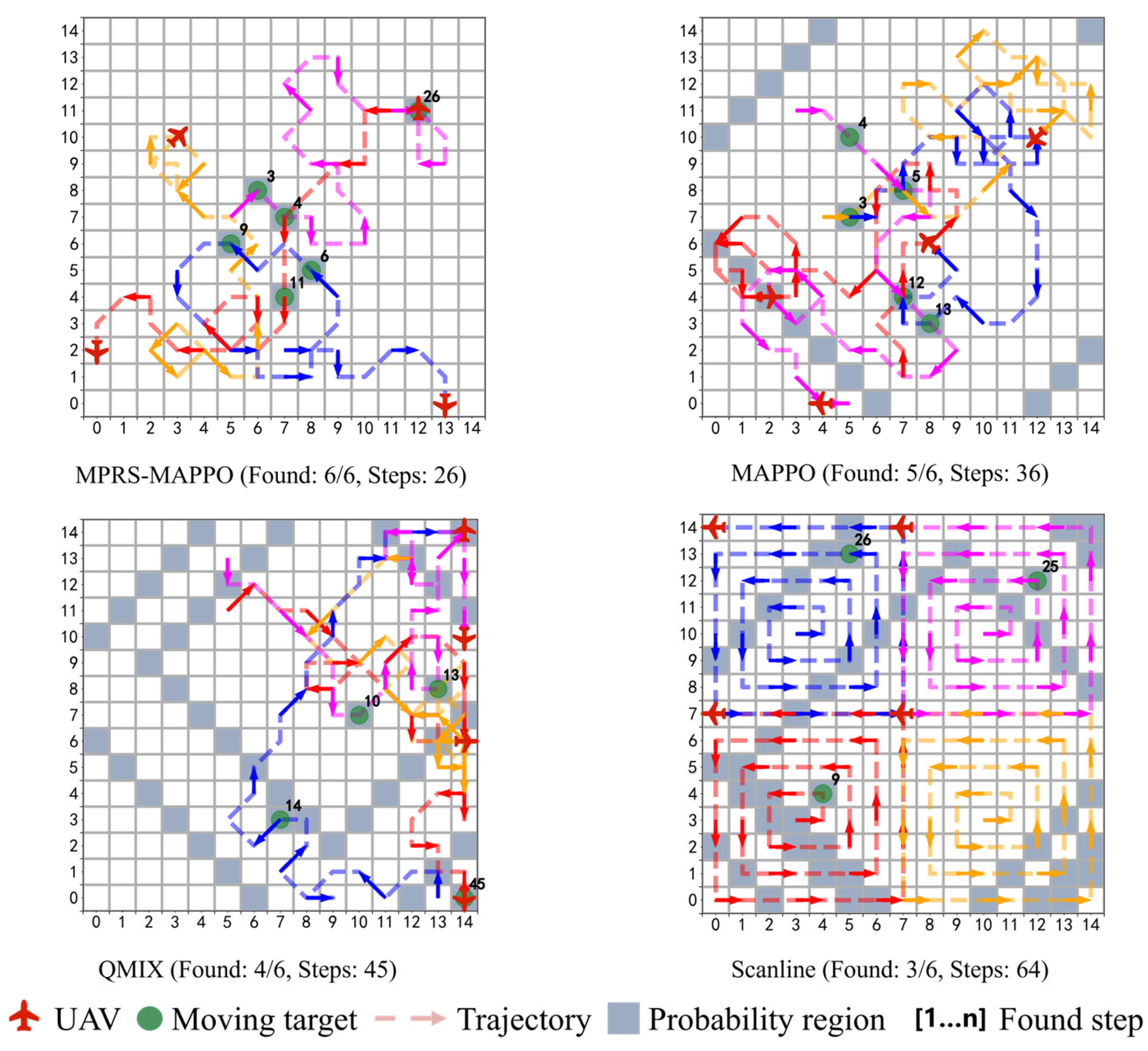
To further analyze behavioral characteristics, the representative search trajectories were visualized, as shown in Figure 14.

Only representative trajectory examples are shown here for clarity; the MASAC trajectories are not displayed due to their similarity in overall pattern to MAPPO. MPRS-MAPPO successfully detected all six targets within only 26 steps, demonstrating a “first concentration, then dispersion” cooperative pattern: initially focusing on high-probability areas, followed by dynamic task allocation to cover wider areas. This reflects advantages in shorter paths and balanced workload distribution. In contrast, MAPPO detected five targets within 36 steps but suffered from uneven workload allocation and missed detections in the later stage. QMIX required 45 steps to detect only four targets, with trajectories biased toward one side and limited utilization of probabilistic information. Scanline detected only three targets after 64 steps due to its static coverage strategy, resulting in the lowest efficiency.

The quantitative comparison is summarized in

Table 3. Performance comparison with existing methods.

Method	Global Return	Detection Rate (%)	Return Std
MPRS-MAPPO	451.43	78.89	9.59
MAPPO	406.85	71.02	10.36
MASAC	395.07	66.83	18.14
QMIX	334.90	61.54	20.56
Scanline	240.91	49.13	21.94

. MPRS-MAPPO achieved significantly higher converged return values and detection rates than the baseline methods, while also maintaining the lowest return standard deviation, indicating superior search efficiency and more stable training performance. In this paper, “training uncertainty” refers to the variability of the cumulative returns during training, which is quantitatively measured by the standard deviation of the returns shown in Table 3.

In summary, MPRS-MAPPO demonstrated clear advantages in multi-UAV cooperative search tasks. It outperformed the baseline methods in terms of convergence speed, target detection rate, and training stability (Return Std), thereby verifying the effectiveness of the adaptive fusion weight mechanism in complex cooperative scenarios. Compared to MAPPO, MASAC, QMIX, and Scanline, MPRS-MAPPO improved target detection rates by 7.87%, 12.06%, 17.35%, and 29.76%, respectively, while reducing training uncertainty by 7.43%, 47.13%, 53.36%, and 56.29%. Future work will explore integrating MHT [46] or PHD [47] tracking to enhance target continuity.

4.4. Ablation Studies

To comprehensively evaluate the MPRS-MAPPO algorithm, two groups of ablation experiments were conducted: one to assess the contribution of each algorithmic component and the other to analyze the cooperative behavior among agents. The first group examines the impact of reward shaping, multi-potential-field fusion, and the warm-up stage on learning performance. The second group explores how partial loss of cooperation affects system efficiency by fixing some UAVs to random policies.

To validate the effectiveness of each component in MPRS-MAPPO, we designed ablation experiments focusing on four aspects:

• The effectiveness of reward shaping;
• Whether multi-potential fields outperform single-potential fields;
• Whether dynamic fusion is superior to fixed fusion;
• The role of the warm-up stage.

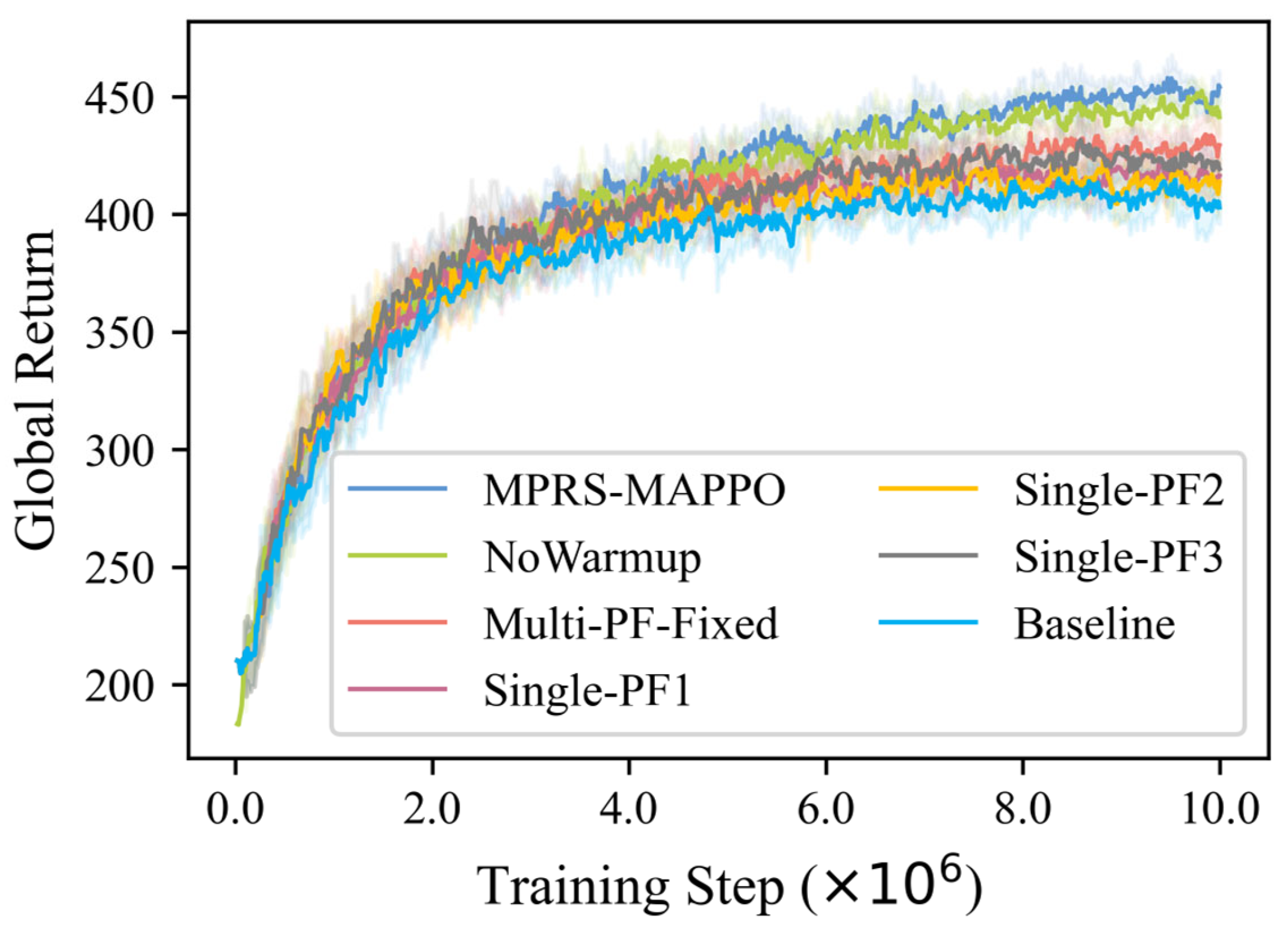
The evaluation metrics included the convergence speed, converged return value, and training stability of the return curves. All methods were implemented on the MAPPO framework under the same environment as in the comparative experiments. As shown in

Table 4. Description of ablation study methods.

Method Name	Description
MPRS-MAPPO	Multi-potential fields + dynamic fusion + warm-up stage (proposed method)
NoWarmup	Multi-potential fields + dynamic fusion, without a warm-up stage
Multi-PF-Fixed	Multi-potential field fusion with fixed weights
Single-PF1	Only Probability Edge Potential Field (${\varphi }^{\mathrm{e}\mathrm{d}\mathrm{g}\mathrm{e}}$)
Single-PF2	Only Maximum Probability Potential Field (${\varphi }^{\mathrm{p}\mathrm{m}\mathrm{a}\mathrm{x}}$)
Single-PF3	Only Coverage Probability Sum Potential Field (${\varphi }^{\mathrm{p}\mathrm{c}\mathrm{o}\mathrm{v}}$)
Baseline	Sparse reward without reward shaping

, the descriptions of the ablation study methods are summarized.

The training return curves of different methods are shown in Figure 15. Overall, MPRS-MAPPO consistently achieved the highest returns with the fastest convergence speed, demonstrating that multi-potential-field fusion and the warm-up stage significantly facilitate policy learning. NoWarmup and Multi-PF-Fixed ranked second and third, respectively, indicating that the warm-up stage further improves training performance and that dynamic fusion is superior to fixed fusion. The single-potential-field methods and the baseline showed much lower returns.

Statistical results of the ablation study are summarized in

Table 5. Statistical results of ablation study.

Method	Global Return	∆Return (%)	Return Std	∆Return Std (%)
MPRS-MAPPO	451.43	11.58	9.59	−7.43
NoWarmup	444.31	9.69	9.86	−4.82
Multi-PF-Fixed	427.87	5.54	9.96	−3.86
Single-PF1	416.82	2.60	10.99	6.08
Single-PF2	413.20	1.74	10.34	−0.19
Single-PF3	422.49	3.98	10.87	4.92
Baseline	406.85	--	10.36	--

.

During convergence, MPRS-MAPPO achieved the highest mean return (an improvement of 11.58%) and the lowest return standard deviation (a reduction of 7.43%), demonstrating superior performance and stability. By contrast, single-potential-field methods provided limited improvements and, in some cases, even introduced instability.

In summary, the adaptive fusion weight mechanism contributed a 5.54% improvement in return; incorporating the multi-potential-field fusion structure further improved the return to 9.69%; and, with the addition of the warm-up stage, the overall return increased by 11.58%. These results convincingly demonstrate the effectiveness and complementarity of reward shaping, multi-potential-field fusion, and the warm-up stage in complex cooperative search tasks.

To further evaluate the impact of inter-agent cooperation, additional experiments were conducted in which a portion of UAVs were fixed to perform random actions, while the remaining UAVs maintained cooperative policy execution.

The results are summarized in

Table 6. Cooperation ablation results under different ratios of cooperative and random UAVs.

Scenario	Cooperative UAVs	Random UAVs	Global Return	Detection Rate (%)	Episode Length
1	4	0	451.43	78.89	40
2	3	1	398.22	69.33	44
3	2	2	342.22	59.49	46
4	1	3	303.47	54.09	47

. As the number of random (non-cooperative) UAVs increased, the overall performance gradually declined. The global return decreased from 451.43 (4 cooperative UAVs) to 303.47 (only 1 cooperative UAV), while the detection rate dropped from 78.89% to 54.09%. Meanwhile, the average episode length increased, reflecting slower mission completion and lower search efficiency due to weakened cooperation.

These results clearly indicate that multi-UAV cooperation plays a critical role in achieving efficient target search and high detection performance.

4.5. Physical Experiments

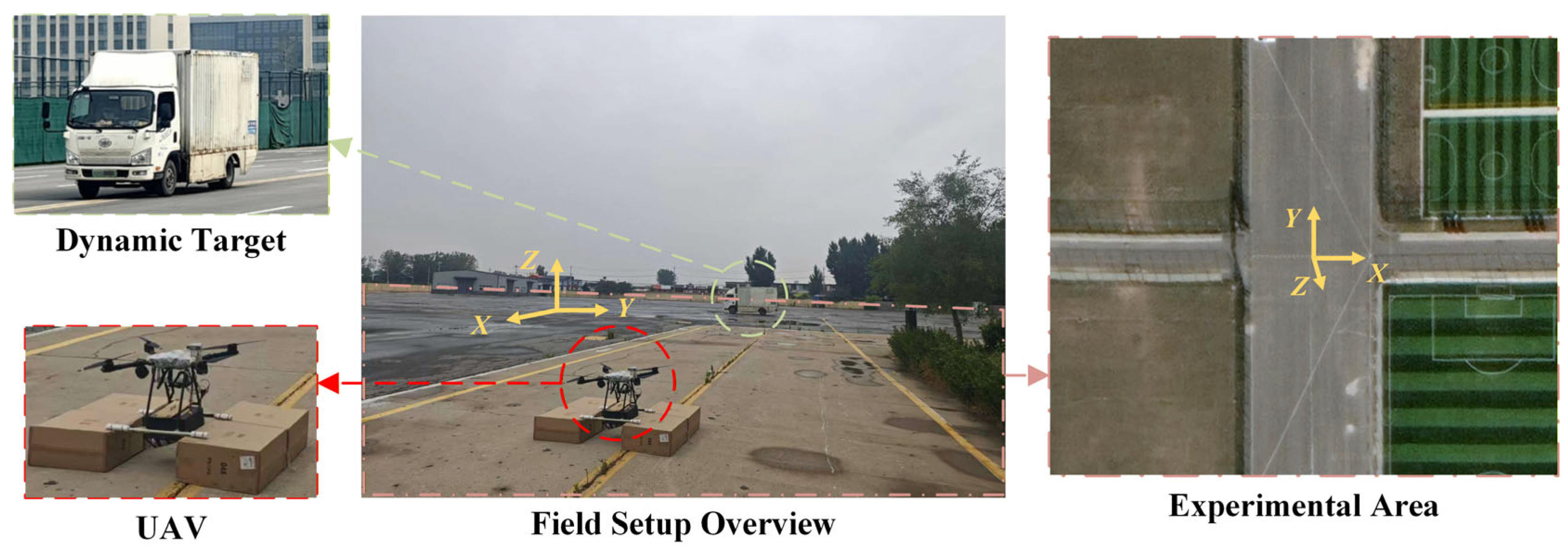
To validate the effectiveness of the proposed algorithm on a real UAV platform, a physical dynamic target search experiment was conducted under laboratory conditions. The setup involved a quadrotor UAV searching for an unknown dynamic target. The UAV was equipped with a visible-light sensor for visual target detection, while the dynamic target was a ground vehicle. Only the target’s initial position was known to the UAV before takeoff. After the experiment started, the vehicle began to move randomly, and the UAV autonomously navigated toward the probabilistic region to search for the target based on the proposed MPRS-MAPPO algorithm. The main experimental parameters are listed in

Table 7. Main Parameters of the Physical Experiment.

Parameter	Value
Area size	100 m × 100 m
Sensor type	visible-light
UAV number	1
Target number	1
UAV speed	15 m/s
Target car speed	5 m/s
UAV flight height	5 m

.

The experimental field setup is shown in Figure 16, where the UAV and dynamic target were deployed in an open area. At the start of the experiment, the target vehicle began to move randomly within the designated region, while the UAV executed the proposed search policy.

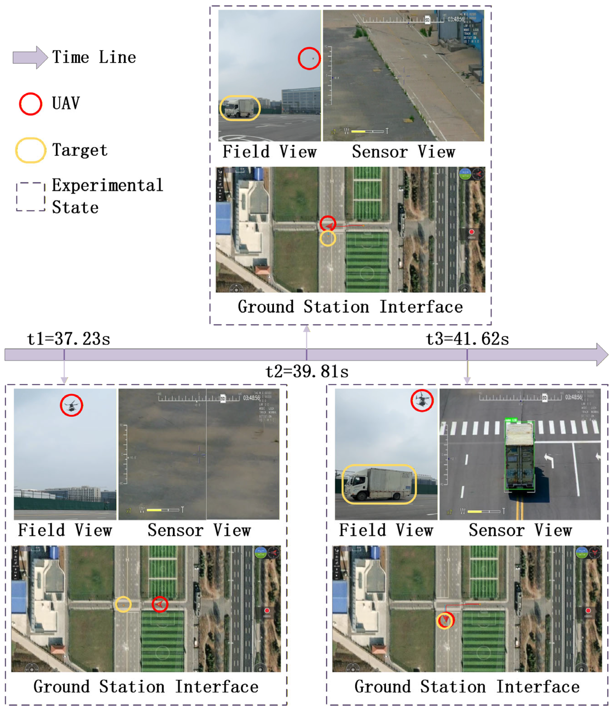
The results of the physical test are illustrated in Figure 17. From left to right, the purple time axis represents the progression of the experiment.

The experimental states at each moment are shown in the dashed boxes aligned with the timeline, including the Field View (real-world scene), Sensor View (onboard camera image), and Ground Station Interface (real-time monitoring).

Search Start (t1 = 37.23 s): The UAV takes off and begins its search. The target is still far away; thus, no vehicle appears in the Field View or Sensor View. The Ground Station Interface shows the UAV and target at their initial positions, separated by a large distance.

Mid Process (t2 = 39.81 s): Both the UAV and target have moved, and the UAV is approaching the high-probability region. However, the target has not yet entered the sensor’s field of view, and no detection is achieved at this stage.

Search Success (t3 = 41.62 s): The UAV maneuvers above the target, and the vehicle becomes visible in the Sensor View. The search is completed successfully, and the task is terminated.

The experimental results confirm that the proposed MPRS-MAPPO algorithm can operate on a real UAV platform and autonomously locate dynamic targets in an outdoor environment. The UAV successfully completed the search mission with accurate navigation and real-time target detection, demonstrating the algorithm’s robustness, real-world feasibility, and potential for practical deployment.

5. Conclusions

This paper addresses the challenges of sparse rewards, unstable training, and inefficient convergence of cooperative strategies in multi-UAV cooperative search for dynamic targets. We propose MPRS-MAPPO, a multi-agent reinforcement learning algorithm that incorporates a multi-potential field fusion reward shaping mechanism. This method is designed for dynamic target search scenarios. It integrates three complementary potential field functions: Probability Edge Potential Field, Maximum Probability Potential Field, and Coverage Probability Sum Potential Field. An Adaptive Fusion Weight Mechanism is adopted for dynamic weight adjustment. In addition, a warm-up stage is introduced to mitigate early-stage misguidance. These designs effectively improve both policy learning efficiency and multi-agent cooperation capability.

Compared with MAPPO, MASAC, QMIX, and the heuristic Scanline method, MPRS-MAPPO achieved notable improvements in convergence speed, global return, and detection rate (by 7.87–29.76%), while reducing training uncertainty by 7.43–56.36%. Ablation studies confirmed that reward shaping, multi-potential-field fusion, and the warm-up stage jointly enhance learning efficiency. Cooperation ablation showed performance degradation when some UAVs used random policies, highlighting the importance of collaboration. Multi-scale (2v3, 4v6, 6v9) and physical flight experiments further verified the algorithm’s scalability, robustness, and real-world applicability.

Future work will focus on extending the framework to more complex and realistic environments to further improve system robustness and practical applicability.