Task Planning and Optimization for Multi-Region Multi-UAV Cooperative Inspection

Highlights

What are the main findings?

• A new multi-region multi-UAV task and path planning model is proposed: the multiple traveling salesmen with neighborhoods problem (MTSPN) model, which integrates the multiple traveling salesmen problem (MTSP) with the traveling salesmen problem with neighborhoods (TSPN).
• A novel decoupled multi-region multi-UAV task and path planning framework has been designed: firstly, the KMGA algorithm—combining K-Means++ algorithm with the genetic algorithm—computes the sequence of task regions to be inspected for each UAV. Subsequently, a multi-neighborhood iterative dynamic programming (MNIDP) algorithm is proposed to solve the multi-neighborhood path planning problem for each UAV.

What are the implications of the main finding?

• This work provides a new multi-UAV task and path planning model, which is solved based on the concept of decoupling.
• The proposed KMGA-MNIDP composite planning strategy could effectively address the multi-region multi-UAV task and path planning problems.

Abstract

To improve the efficiency of multi-region multi-unmanned aerial vehicle (UAV) inspection, this paper proposes a composite task planning strategy integrating the K-Means++ genetic algorithm (KMGA) and the multi-neighborhood iterative dynamic programming (MNIDP) method. Firstly, the multi-region multi-UAV inspection problem is modeled as a multiple traveling salesmen problem with neighborhoods (MTSPN). Then, this problem is decomposed into two interrelated subproblems to mitigate the complexity inherent in the solution process: that is, the multiple traveling salesmen problem (MTSP) and multi-neighborhoods path planning (MNPP) problem. Based on this decomposition, the MTSP is solved by the KMGA by converting it into m spatially non-overlapping traveling salesmen problems (TSPs) and then these TSPs are solved to obtain the approximate optimal visiting sequences for the nodes in each TSP in a short time. Subsequently, the MNPP can be efficiently solved by an MNIDP which plans the paths between the corresponding neighborhood of each node based on the node visiting sequences, thus obtaining the approximate optimal path length of the MTSPN. The simulation results demonstrate that the proposed composite strategy exhibits advantages in computational efficiency and optimal path length. Specifically, compared to the baseline algorithm, the average tour length obtained by the KMGA decreased by 23.24%. Meanwhile, the average path lengths computed by MNIDP in three instances were reduced from 8.00% to 11.41% and from 6.46% to 10.08% compared to two baseline algorithms, respectively. It provides an efficient task and path planning solution for multi-region multi-UAV operations in power transmission line inspections, thereby enhancing inspection efficiency.

1. Introduction

With the continuous advancement of industrialization, new power systems integrating multiple energy sources have replaced traditional grids as the mainstream development model [1]. New energy sources, primarily wind and solar power, are widely distributed across vast hilly and desert regions, forming AC/DC microgrids with surrounding power facilities [2,3]. The expansion of new energy power systems has led to an increase in transmission lines, thereby complicating their inspection processes. Consequently, while the traditional manual inspection remains the mainstream method for the transmission line inspections, the use of the unmanned aerial vehicles (UAVs) is gradually increasing. Beyond infrastructure inspection, UAV swarms hold significant promise for other complex missions. For instance, in addressing today’s pressing air pollution challenges, multi-UAV systems can generate consistent horizontal pollution maps and vertical profiles across vast areas [4]. UAV-based inspection is a multi-UAV multi-target task planning and optimization problem. The problem is characterized by multiple constraints (such as intermittent communication in networked UAV cooperation [5]) and is a non-deterministic polynomial-hard (NP-hard) problem [6].

The multiple traveling salesman problem (MTSP) model is a classic method for addressing the problem of multi-UAV multi-target cooperative task planning. It frames UAVs as traveling salesmen and inspection targets as travel destinations. MTSP is an extension of the traveling salesman problem (TSP), and it differs from the TSP in that there are m salesmen, rather than one, who need to visit n cities (n > m).

Current approaches to solving the MTSP predominantly utilize heuristic and metaheuristic algorithms. Early foundational work by Rusell (1977) proposed a methodology that transforms the MTSP into a standard TSP, subsequently solved using the Lin–Kernighan algorithm, yielding relatively accurate solutions [7]. With the advancement of heuristic optimization algorithms (such as particle swarm optimization, bat algorithm, and cuckoo search) [8], the research on the MTSP has rapidly progressed. Building upon these foundations, a variety of methods were introduced by the researchers. For instance, Pan successfully employed the ant colony optimization algorithm to address the capacity-constrained MTSP, obtaining favorable experimental results [9]. Carter et al. developed an efficient solution using a genetic algorithm, which features a specifically designed two-part chromosome structure and tailored genetic operators (TPCGA) [10]. Zhang et al. introduced a hybrid method, which combines the solution space generated by elementary matrix operations with the state transition-simulated annealing algorithm and 2-opt local search for the solution. This method shows a statistically superior optimization performance [11]. In [12], a modified Two-Part Wolf Pack Search algorithm incorporating a two-part encoding scheme was proposed to address MTSP directly, and the experiments confirm its solution quality exceeded that of two comparative algorithms. For multiple depots MTSP, Hu et al. presented an approach combining fuzzy C-means clustering with an improved partheno-genetic algorithm for solving individual TSPs [13]. More recently, Modares [14], Qu [15], and others [16,17] have explored solving MTSP using neural network models. Although these neural approaches can provide good solutions, they often suffer from prohibitively long search times. Some research on drone task assignments can also be applied to address the MTSP. The reference [18] presents an innovative approach to solving task allocation optimization, where the algorithm selects an appropriate subset of operators to execute a given task, driven primarily by algorithmic efficiency and maximizing task success. The experiments demonstrate that this method achieves a significantly improved performance compared to other approaches.

Note that, in some situations, the UAV just needs to reach the region near each target rather than the target itself to complete the task [19]. This problem can be expressed as a variant of TSP named the traveling salesman problem with neighborhoods (TSPN). Therefore, the multi-UAV multi-target task planning and optimization problem can be transformed into the multi-region multi-UAV cooperative task planning and optimization problem. Existing works have categorized cooperative structures for this problem into open-loop, closed-loop (centralized/distributed), and space cooperation [20], laying the foundation for strategy design. Modifying the inspection strategy from requiring arrival at specific points to arrival within predefined areas significantly reduces the energy consumption and inspection time of UAVs.

Significant research exists on the TSPN. Gentilini et al. formulated the TSPN as a non-convex mixed-integer nonlinear program and effectively solved it using the COIN-OR solver [21]. Subsequent work by Gentilini and Vicencio et al. extended the TSPN to the generalized TSP with neighborhoods and proposed a hybrid random-key genetic algorithm to address this problem [22]. Xin et al. [19,23,24,25,26,27] have proposed a series of algorithms for solving the Dubins traveling salesman problem with neighborhoods, yielding good results. In [28], a generalized Benders decomposition is proposed as a solution to the pickup-and-delivery traveling salesman problem with convex and non-convex neighborhoods. Clark developed two convex relaxation algorithms for the metric TSP: one is based on a heuristic method, and the other is based on a submodular optimization approach using a minimum spanning tree [29]. In [30], an unsupervised learning algorithm based on growing self-organizing arrays is proposed for solving the traveling salesman problem with neighborhoods on a sphere. Puerto et al. provide the mathematical programming formulations for the traveling salesman problems with neighborhoods and barriers [31].

The aforementioned works on the TSPN have mostly focused on single-agent scenarios, while the research on multi-agent scenarios is relatively scarce. To address this gap, a composite strategy is proposed in this work. The main contributions of this work are summarized as follows:

(1)

A model addressing multi-region multi-UAV mission and path planning problems is proposed, which is decomposed into two subproblems: MTSP and MNPP (a TSPN variant targeting optimal paths to visit all neighborhoods per preset sequence). This modeling approach effectively decouples the solution process, avoiding the computational complexity associated with direct coupled solutions.

(2)

A K-Means++ genetic algorithm (KMGA) combining K-Means clustering with genetic algorithms is proposed. It addresses the downside of MTSPN that only focuses on the path cost (ignoring UAV collision avoidance) and the inability of existing heuristic algorithms to solve these shortcomings.

(3)

A multi-neighborhood iterative dynamic programming (MNIDP) algorithm based on dynamic programming principles is proposed. It achieves shorter path lengths compared to baseline methods when solving the MNPP problem.

(4)

A series of comparative simulations are conducted. The simulation results demonstrated that the proposed composite decoupling planning framework can effectively enhance the inspection efficiency of multi-region multi-UAV operations in transmission lines.

The rest of the paper is organized as follows: Section 2 constructs models for the MTSP and MNPP, respectively, and derives the model for the MTSPN. Section 3 and Section 4 introduce the KMGA and the MNIDP proposed in the paper. Section 5 describes the setup, results, and analysis of the simulations. Section 6 provides a conclusion and the future work on the MTSPN. Please note that the UAVs considered in this paper are quadrotor UAVs

2. Problem Description

This section introduces the models for the MTSP and the MNPP, respectively, and ultimately derives the problem model for MTSPN.

Assume there is a complete graph topology for all test instances. Specifically, every pair of distinct inspection points is directly connected by a unique edge, and the edge weight represents the Euclidean distance between these points.

2.1. Description of MTSP

The specific definition of MTSP has been given in the previous section. If the Euclidean norm is employed as a distance function, the MTSP becomes symmetric. The objective of the MTSP description presented herein is to minimize the total path length traversed by all m salesmen. Accordingly, the symmetric MTSP is formulated as follows:

$$\mathrm{minimize}: {\displaystyle \sum _{k=1}^m{\displaystyle \sum _{i=1}^n{\displaystyle \sum _{j=1}^n{d}_{ij}{x}_{ijk}}}}$$

(1)

$$\hspace{1em}\hspace{1em}\hspace{1em}\hspace{1em}\hspace{1em}\hspace{1em}\mathrm{subject} \mathrm{to}: {\displaystyle \sum _{k=1}^m{y}_i^k=1}\hspace{1em}\hspace{1em}\hspace{1em}\forall i\in [1,n]$$

(2)

$$\hspace{1em}\hspace{1em}\hspace{1em}\hspace{1em}\hspace{1em}\hspace{1em}\hspace{1em}\hspace{1em}\hspace{1em}\hspace{1em}\hspace{1em}{\displaystyle \sum _{j=1}^n{x}_{ijk}=1\hspace{1em}\hspace{1em}\hspace{1em}\forall k\in [1,m]}$$

(3)

$$\hspace{1em}\hspace{1em}\hspace{1em}\hspace{1em}\hspace{1em}\hspace{1em}\hspace{1em}\hspace{1em}\hspace{1em}\hspace{1em}\hspace{1em}{\displaystyle \sum _{i=1}^n{x}_{ijk}=1\hspace{1em}\hspace{1em}\hspace{1em}\forall k\in [1,m]}$$

(4)

$$\hspace{1em}\hspace{1em}\hspace{1em}\hspace{1em}\hspace{1em}\hspace{1em}\hspace{1em}{\displaystyle \sum _{k=1}^m{\displaystyle \sum _{i=1}^n{y}_i^k=m+n }}$$

(5)

where n is the number of the cities, m is the number of the salesmen, d_ij is the Euclidean distance between city i and city j, x_ijk is a binary variable that indicates whether salesman k travels from city i and city j, and y_i^k is a binary variable that indicates whether salesman k has visited city i.

The problem constraint in (2) ensures each city can only be visited by one salesman once. The problem constraints in (3) and (4) ensure that each salesman must start from a start city and return to it. The problem constraint in (5) ensures the sum of the cities visited by all salesmen is n and each salesman returns to its start city.

In this paper, the MTSP is defined as follows: m salesmen depart from m distinct initial cities, each required to visit a subset of cities, and return to their own starting city. Each city in the set must be visited exactly once by exactly one salesman. Furthermore, considering that the UAVs performing transmission line inspections are typically deployed from a common depot, the m cities closest to this depot are selected as the starting cities. The depot is randomly placed in an area distant from all inspection nodes in this paper. And in practice, the specific location of the depot is determined by actual conditions. Accordingly, (1) is adapted as follows:

$$\mathrm{minimize}: {\displaystyle \sum _{k=1}^m{\displaystyle \sum _{i=1}^n{\displaystyle \sum _{j=1}^n{d}_{ij}{x}_{ijk}}}}+{\displaystyle \sum _{k=1}^m{d}_k}$$

(6)

where d_k is the Euclidean distance between the starting city k and the depot.

2.2. Description of MNPP

It is assumed that there exist n convex neighborhoods. This assumption offers the following key advantages:

(1)

Simplicity of computation: For convex neighborhoods, it is simple to calculate the optimal path points of the UAVs. This scenario can typically be transformed into a more straightforward geometric problem rather than a complex optimization problem, which greatly reduces computational complexity.

(2)

Theoretical solvability: This assumption enables many classical optimization algorithms which are initially designed for the standard TSP or MTSP and could be adapted for addressing the MTSPN.

(3)

Easy to model: It is straightforward and intuitive to represent the neighborhoods via convex polygons such as circles, ellipses, and squares, facilitating the rapid construction of test instances and verification of algorithm performance.

The d (p_i, p_j) is used to represent the distance between a point in neighborhood i and a point in neighborhood j. Therefore, the MNPP can be formulated by the following:

$$\mathrm{minimize}: {\displaystyle \sum _{i=1}^n{\displaystyle \sum _{\begin{array}{l}j=1\\ j\ne i\end{array}}^{n}d(p_i,p_j)x_{ij}}}$$

(7)

$$\hspace{1em}\hspace{1em}\hspace{1em}\hspace{1em}\mathrm{subject} \mathrm{to}: {\displaystyle \sum _{\begin{array}{l}j=1\\ j\ne i\end{array}}^n{x}_{ij}=1\hspace{1em}\hspace{1em}\hspace{1em}\forall i\in [1,n]}$$

(8)

$$\hspace{1em}\hspace{1em}\hspace{1em}\hspace{1em}\hspace{1em}\hspace{1em}\hspace{1em}\hspace{1em}\hspace{1em}{x}_{ij}+x_{jl}\ge x_{il}\hspace{1em}\hspace{1em}\hspace{1em}\forall i,j,l\in [1,n]$$

(9)

where i, j, and l are the neighborhoods, p_i and p_j represent path points selected from the neighborhood i and j, and x_ij is a binary variable that indicates whether the path passes through p_i and p_j.

The problem constraint in (8) ensures that each neighborhood can be visited once. The triangular inequality constraint in (9) ensures the continuity of the path.

2.3. Construction of MTSPN Model

The previous sections formalize the MTSP under Euclidean distance, minimizing the total route length for m agents departing from distinct starting cities, and introduce the MNPP, which optimizes a continuous path visiting one point in each convex neighborhood. The MTSPN model is derived from the descriptions of the MTSP and MNPP, respectively. Its complete mathematical formulation is given below:

$$\mathrm{minimize}: {\displaystyle \sum _{k=1}^m{\displaystyle \sum _{\begin{array}{l}j=1\\ j\ne i\end{array}}^n{\displaystyle \sum _{i=1}^{n}d(p_i,p_j)x_{ijk}}}}+{\displaystyle \sum _{k=1}^m{d}_k}$$

(10)

$$\mathrm{subject} \mathrm{to}: {\displaystyle \sum _{k=1}^m{y}_i^k=1}\hspace{1em}\hspace{1em}\hspace{1em}\forall i\in [1,n]$$

(11)

$$\hspace{1em}\hspace{1em}\hspace{1em}\hspace{1em}\hspace{1em}\hspace{1em}\hspace{1em}\hspace{1em}\hspace{1em}\hspace{1em}\hspace{1em}{\displaystyle \sum _{\begin{array}{l}j=1\\ j\ne i\end{array}}^n{x}_{ijk}=1\hspace{1em}\hspace{1em}\hspace{1em}\forall k\in [1,m]},\forall i,j\in [1,n]$$

(12)

$$\hspace{1em}\hspace{1em}\hspace{1em}\hspace{1em}\hspace{1em}\hspace{1em}\hspace{1em}\hspace{1em}\hspace{1em}\hspace{1em}\hspace{1em}{\displaystyle \sum _{i=1}^n{x}_{ijk}=1\hspace{1em}\hspace{1em}\hspace{1em}\forall k\in [1,m]},\forall i,j\in [1,n]$$

(13)

$${\displaystyle \sum _{k=1}^m{\displaystyle \sum _{i=1}^n{y}_i^k=m+n}}$$

(14)

$$\hspace{1em}\hspace{1em}\hspace{1em}\hspace{1em}\hspace{1em}\hspace{1em}\hspace{1em}{x}_{ij}+x_{jl}\ge x_{il}\hspace{1em}\hspace{1em}\hspace{1em}\forall i,j,l\in [1,n]$$

(15)

3. K-Means++ Genetic Algorithm

In this paper, the K-Means++ genetic algorithm is proposed to solve MTSP by converting to solving m times TSP. The algorithm commences by partitioning the set of n cities into m clusters via the K-Means++ algorithm. Subsequently, the genetic algorithm is applied to solve the individual TSP for each cluster. The final MTSP solution is synthesized by aggregating these independent TSP results.

3.1. K-Means++ Clustering Algorithm

The K-Means algorithm is an unsupervised clustering method widely used in data mining and machine learning. It aims to partition a given dataset into K distinct clusters by maximizing intra-cluster similarity and inter-cluster dissimilarity.

The core objective of the algorithm is to minimize intra-cluster variance, which is measured by the sum of squared Euclidean distances between each data point and the centroid of its assigned cluster. Formally, given a dataset D of n samples, the algorithm aims to partition the data into K clusters C = {C₁, C₂, …, C_K} that minimize the following objective function:

$$E={\displaystyle \sum _{i=1}^K{\displaystyle \sum _{x\in C_i}{‖x-{\mu }_i‖}^2}}$$

(16)

where μ_i is the centroid of cluster C_i, and ||x − μ_i|| represents the Euclidean distance between the sample point x and the centroid μ_i.

Standard K-Means are highly sensitive to the initial selection of centroids, frequently converging to local optima rather than the global optimum. To address this limitation, the K-Means++ algorithm is employed [32], and it improves centroid initialization through a probabilistic seeding mechanism that spreads initial centroids based on a weighted probability distribution.

(1)

Randomly select the first centroid c₁ from the dataset.

(2)

For each subsequent centroid c_k (k = 2, …, K), the selection probability for each unselected point is computed, and the next centroid c_k is then sampled proportionally to P(x_i):

$$P(x_i)={\displaystyle \frac{d^2(x_i,c_{selected})}{{\displaystyle {\sum }_{x_j\notin c_{selected}}{d}^2(x_j,c_{selected})}}}$$

(17)

where x_i and x_j are the i th and j th data points, c_selected is the selected centroid, and d (x_i, c_selected) is the minimum distance from x_i to any existing centroid.

Following the initialization of all K centroids, the K-Means++ algorithm follows the same iterative procedure as the standard K-Means algorithm: (i) assigning each point to its nearest centroids and (ii) updating centroids until convergence (centroid stability) or a preset iteration limit is reached.

3.2. The Implementation of Genetic Algorithm

The Genetic Algorithm (GA) is a heuristic optimization technique inspired by biological evolution, which iteratively improves solutions through simulated genetic operations. Our implementation incorporates four core components:

Chromosome Representation: Each chromosome encodes a candidate path as an ordered gene sequence. The k-th gene G_k corresponds to node k’s Cartesian coordinates (x_k, y_k):

$$G_k=(x_k,y_k)$$

(18)

This representation enables the direct Euclidean distance calculation between nodes.

Population Initialization: In this paper, the standard nearest neighborhood algorithm is employed to generate a high-quality initial population.

(1)

Randomly select starting node i.

(2)

Find unvisited node j minimizing the distance:

$$j=\underset{j\in C}{\arg \min }(d_{ij})$$

(19)

where C denotes unvisited nodes and d_ij is the distance between node i and node j.

(3)

Update current node: i←j.

(4)

Repeat steps 2–3 until all nodes are visited.

To provide the genetic algorithm with an initial population that is both high-quality and diverse, we employ a multi-start strategy: running the nearest neighbor heuristic multiple times, each time randomly selecting a different city as the starting point. This generates multiple distinct initial paths to construct the initial population. This approach combines the efficiency of heuristic algorithms with the diversity maintained through randomness, aiming to provide an excellent starting point for subsequent genetic evolution.

Fitness Function: Solution quality is evaluated by

$$f(c_i)={\displaystyle \frac{1}{D_i}}+\lambda \cdot \varphi (D_i)$$

(20)

where D_i is the total path length on the ith chromosome, 1/D_i rewards shorter path lengths D_i, and λ is a negative number named the penalty factor.

The D_threshold represents the threshold value and the penalty function is as follows:

$$\varphi (D_i)=\left\{\begin{array}{l}0\hspace{1em}\hspace{1em}\hspace{1em}\hspace{1em}\hspace{1em} D_i\le D_{threshold}\\ {\displaystyle \frac{1}{D_i-D_{threshold}}}\hspace{1em}{D}_i>D_{threshold}\end{array}\right.$$

(21)

The D_threshold is defined as the average path length of all chromosomes in the population, a setting that serves as an effective discriminant for chromosome quality. By taking this population-level statistic as the benchmark, the algorithm inherently prioritizes the top 50% of high-quality chromosomes and guarantees them a significantly higher probability of being selected for inheritance, thus preserving their advantageous traits in subsequent generations.

The parameter λ is set to −0.1, a value carefully calibrated to strike a balance between evolutionary progress and diversity. This negative value ensures that high-quality chromosomes maintain their dominant role in inheritance, preventing the erosion of proven advantageous characteristics. Simultaneously, it reserves a modest opportunity for low-quality chromosomes to be inherited, introducing necessary variability that enriches the population’s genetic diversity and mitigates the risk of premature convergence.

Genetic Operator: The genetic operators include three operators: selection operator, crossover operator, and mutation operator.

(1)

Selection Operator: The roulette wheel algorithm is employed as the selection operator, and a dynamic factor α is incorporated to prevent the algorithm from falling into the local optimal solution. The improved probability p(c_i) of each chromosome that is selected is as follows:

$$p(c_i)={\displaystyle \frac{f(c_i)+\alpha }{({\displaystyle \sum _{i=1}^{m}f(c_i))+\alpha }}}$$

(22)

(2)

Crossover Operator: The partially matched crossover method.

(3)

Mutation Operator: The bit flip operation. In order to reduce the mutation probability of high-quality chromosomes and increase the probability of the low-quality chromosomes, this paper employs the adaptive mutation probability p_m proposed in previous research:

$$p_m=\left\{\begin{array}{l}{p}_{m0}\cdot {\displaystyle \frac{f_{max}-f}{f_{max}-f_{avg}}}, f>f_{avg}\\ p_{m0}\cdot {\displaystyle \frac{f_{max}-f_{\mathrm{avg}}}{f-f_{min}}}, f<=f_{avg}\end{array}\right.$$

(23)

where p_m0 is the basic mutation probability, f is a simplified expression of f(c_i), and f_max, f_min, and f_avg are the maximum, the minimum, and average values of the fitness of the chromosomes in the population, respectively.

By integrating the K-Means++ algorithm with the genetic algorithm devised in this paper, the MTSP can be decomposed into m independent TSP subproblems, and each TSP is solved separately. The specific process of the algorithm is the same as Algorithm 1.

The hyperparameters of the genetic algorithm employed in this paper are shown in

Table 1. The hyperparameters of the genetic algorithm.

Hyperparameters	Value
population size	80
crossover rate	0.8
mutation rate	0.1
number of generations	500

, and the algorithm stops after reaching the number of generations.

Algorithm 1 A K-Means++ Genetic Algorithm for solving MTSP

1: Input: the locations of n cities: data, the number of salesmen: m, the UAV parking place: origin

2:  procedure K-Means++ Cluster (data, n)

3:    center1 = random (data) 4:     initialize rest m − 1 center

5:     repeat

6:     assign center for ci and gain cluster cli

7:      centeri = mean (data(ci)) for cli

8:     end repeat until maximum iterations

9:   end procedure

10: for cli

11:    select the start point

13:    procedure GA (data(cli))

14:      initialize population

15:      repeat

16:        calculate fitness of each chromosome

17:        selection, crossover and mutation

18:      end repeat until maximum iterations

19:    end procedure

20: Output: solution of MTSP

4. Multi-Neighborhoods Iterative Dynamic Programming

Leveraging the K-Means++ GA method introduced in the preceding section, the MTSP instance is decomposed into m independent TSP subproblems, for each of which the optimal node visitation order is computed. Subsequently, the multi-neighborhood iterative dynamic programming algorithm is proposed to determine the optimal path points within the neighborhood of each node based on the predetermined visitation sequence.

4.1. Dynamic Programming for MNPP

The MNPP studied in this paper exhibits the two essential properties that make it amenable to dynamic programming (DP): optimal substructure and overlapping subproblems.

Optimal Substructure in MNPP: The optimal path from any starting neighborhood i to a target neighborhood k can be constructed by optimally combining the paths from i to an intermediate neighborhood j and from j to k. This property allows the global MNPP to be decomposed into a sequence of smaller, interrelated subproblems.

Overlapping Subproblems in MNPP: During the computation, the solution to the subproblem involving paths between i and j will be reused multiple times when solving for different target neighborhoods k. This makes DP—which stores solutions to subproblems in a table to avoid redundant computations—particularly efficient for MNPP.

Given the aforementioned properties, DP is employed to solve the MNPP. The core of our approach involves:

(1)

State Definition: The state d_p(i, k) represents the optimal cost (or key metric) for the path from the starting neighborhood i to neighborhood k.

(2)

State Transition Equation: The equation d_p(i, k) = min{d_p(i, k) + cost(j, k)} (or a variant thereof) systematically builds the solution for larger paths by combining the solutions of smaller overlapping sub-paths.

(3)

Initialization: The base cases are defined, such as d_p(i, k) = 0, for the path from any neighborhood to itself.

4.2. Multi-Neighborhood Iterative Dynamic Programming

As stated in Section 4.1, the dynamic programming algorithm is suitable for solving the MNPP researched in this paper. Based on the idea of the dynamic programming algorithm, this paper employs the MNIDP to address the aforementioned problem. The specific process of the algorithm is the same as Algorithm 2.

Certain specific steps in this algorithm will be elaborated in detail below:

Path Node Initialization: For each neighborhood i, an initial path node is selected. In this work, the center of the neighborhood is adopted as the initial path node, and the path derived from this initialization approach is consistent with the path computed by the KMGA.

Neighborhood Discretization: To define the initial regional space and movement direction of optimal path nodes, neighborhood discretization is performed in this study. To streamline computations, a uniform discretization strategy for neighborhood boundaries is first adopted to generate a candidate node set. Subsequently, by computing the sum of Euclidean distances between each discretized node and the path nodes of the preceding and subsequent neighborhoods, the discretized node with the minimum distance sum is selected as the new path node.

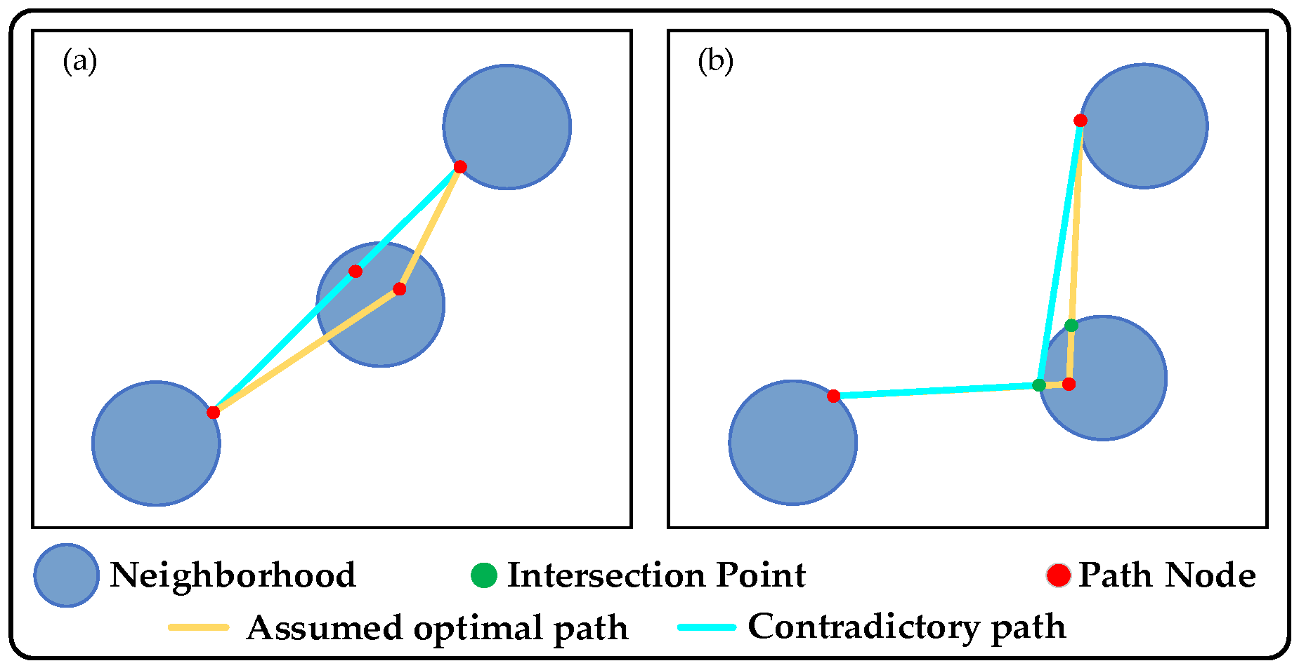
Path Node Selection: Note that the existing forms of the shortest path nodes in the neighborhood are exclusively limited to two cases (as shown in Figure 1):

Case (a): When the connecting segment between the path nodes of adjacent neighborhoods intersects with the current neighborhood, all points along this segment within the current neighborhood satisfy the path node condition. The midpoint of the segment inside the neighborhood is selected as the path node in the paper.

Case (b): The path node lies on the boundary of the neighborhood. The majority of instances fall into case (b).

Proof. 

The proof of case (a) is as follows (as shown in Figure 2a):

Assume there exists a shortest path point p_i that does not lie on the connection its adjacent path points p_i−1 and p_i+1 but instead locates at another position in the current neighborhood. Connect p_i with its preceding and succeeding path points p_i−1 and p_i+1, respectively, and then connect p_i−1 with p_i+1, forming triangle ${△}_{p_{i-1}{p}_i{p}_{i+1}}$. According to the triangle inequality in Euclidean space, the length of the connection p_i−1 p_i+1 satisfies the following:

$$d(p_{i-1},p_{i+1})\le d(p_{i-1},p_i)+d(p_i,p_{i+1})$$

(24)

Given the non-collinear assumption of p_i−1, p_i, and p_i+1, this inequality holds strictly:

$$d(p_{i-1},p_{i+1})<d(p_{i-1},p_i)+d(p_i,p_{i+1})$$

(25)

The result indicates that the path p_i−1→p_i+1 has a shorter length than the path p_i−1→p_i→p_i+1, contradicting the assumption. Therefore, the shortest path points must lie on the connection between adjacent path points, thus verifying the correction of case (a). □

Proof. 

The proof of case (b) is as follows (as shown in Figure 2b):

Select an internal path node p_i within the current neighborhood (excluding boundaries); connect p_i with adjacent path points p_i−1 and p_i+1. The resulting connections intersect the neighborhood boundary at points b₁ and b₂. Connect p_i+1 and b₁, and by the triangle inequality, it follows that

$$d(p_{i-1},b_1)+d(b_1,p_{i+1})<d(p_{i-1},p_i)+d(p_i,p_{i+1})$$

(26)

Equation (30) contradicts the assumption that p_i is the shortest path node, thereby proving case (b). □

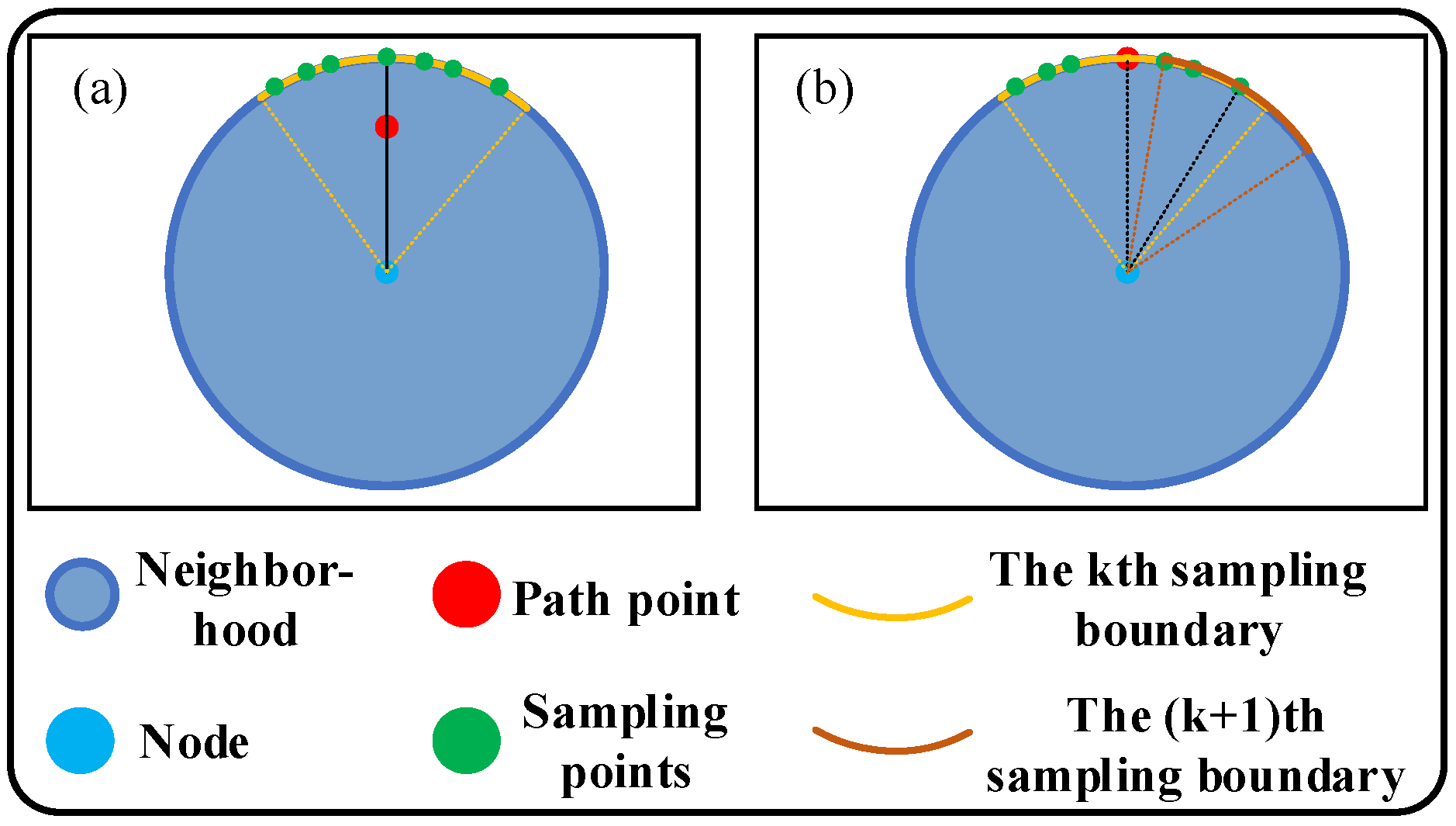
Path Node Vicinity Sampling: For the two cases described above, there exist corresponding sampling methods (as illustrated in Figure 3):

Case (a): Connect the node to the midpoint of the adjacent segment and extend this line until it intersects with the neighborhood boundary. Then, randomly sample a segment of the boundary near the intersection point, and include the intersection point itself in the candidate point set.

Case (b): When the connecting line between path nodes in two adjacent neighborhoods does not intersect with the current neighborhood, the feasible path nodes are constrained to lie on the neighborhood boundary. Accordingly, random sampling is performed along a segment of the boundary near the original path point, and the path point is also directly added to the sampling set.

As the iteration progresses, the boundary segment subject to sampling gradually narrows until the iteration concludes.

Algorithm 2 Multi-Neighborhood Iterative Dynamic Programming Algorithm for Solving MNPP

1:  Input: the locations of a nodes with known node order: loc, the radius of the region: r, the maximum iterations: itemax

2:   procedure iterative dynamic programming

3:      initialize the path node pi(0) of each neighborhood Ni

4:      discretize the neighborhoods and gain $\left\{p_i^{(0,j)}\right\}$

5:      for i = 1: a do

6:       if the connection between pi−1 and pi+1 crosses Ni

7:         pi(0) = midpoint of the in-neighborhood part of the connection

8:       end if

9:      $p_i^{(1)}=\arg \underset{p\in \left\{p_i^{(0,j)}\right\}}{\min }(‖p_{i-1}^{(1)}-p‖+‖p-p_{i+1}^{(0)}‖)$

10:   end for

11:    while the iteration number k < itemax do

12:       for i = 1: a do

13:         if the connection between pi−1 and pi+1 crosses Ni

14:          pi(k+1) = midpoint of the in-neighborhood part of the connection

15:        end if

16:         sample the area of a specified size around pi and obtain a set of sampling points $\left\{p_i^{(k,j)}\right\}$; then add pi(k) to $\left\{p_i^{(k,j)}\right\}$

17:        $p_i^{(k+1)}=\arg \underset{p\in \left\{p_i^{(k,j)}\right\}}{\min }(‖p_{i-1}^{(k+1)}-p‖+‖p-p_{i+1}^{(k)}‖)$

18:      end for

19:    end while

20:  end procedure

21:  Output: solution of MNPP

The following is the discussion about the time and space complexity of the MNIDP algorithm:

Assume that there are n neighborhoods. The time complexity of the algorithm is first discussed. Since the selection of discrete points occurs only at the boundaries of neighborhoods and only needs to calculate the distance between each discrete point in each neighborhood and the path points in adjacent neighborhoods, the number of points is proportional to the perimeter of the neighborhood. Thus, the time complexity is O(r + 2) = O(r). With n neighborhoods, the total discrete time is O(n × r). The path node initialization operation is performed n times, resulting in an initialization time of O(n). Thus, the total time per iteration is O(n × r + n) = O(n × r). Given the maximum iterations ite_max, the final time complexity of the MNIDP algorithm is O(ite_max × n × r).

Next is the discussion of the space complexity of the algorithm. The algorithm requires storing the following data: each neighborhood contains O(r) points after discretizing neighborhood, and there are n neighborhoods, so the storage space is O(n × r). Storing the information for n path nodes requires O(n) space; during the iteration process, each sampling requires storing O(r) points; however, since sampling is performed domain-by-domain, only the current sampled point set needs temporary storage, resulting in a sampling space of O(r). Therefore, the space complexity of the MNIDP algorithm is O(n × r) + O(n) + O(r) = O(n × r).

Proof. 

The proof of the convergence of the MNIDP algorithm is as follows:

During each iteration, select the point from the candidate points that minimizes the total length of the adjacent path segments:

$$p_i^{(k+1)}=\arg \underset{p\in \left\{p_i^{(k,j)}\right\}}{\min }(‖p_{i-1}^{(k+1)}-p‖+‖p-p_{i+1}^{(k)}‖)$$

(27)

Since p_i^(k) is included in the set of the candidate points, it follows that

$$‖p_{i-1}^{(k+1)}-p_i^{(k+1)}‖+‖p_i^{(k+1)}-p_{i+1}^{(k)}‖\le ‖p_{i-1}^{(k+1)}-p_i^{(k)}‖+‖p_i^{(k)}-p_{i+1}^{(k)}‖$$

(28)

Sum over all neighborhoods and obtain

$$L^{(k+1)}\le L^{(k)}$$

(29)

Therefore, the objective function (the total path length) L^(k) is a non-increasing sequence. Meanwhile, it is evident that L^(k) ≥ 0 and has a lower bound (the length of the optimal path).

According to the Monotone Convergence Theorem: If the sequence {L^(k)} is non-increasing and bounded below, then it must converge to a certain limit L^*:

$$\underset{k\to \infty }{\lim }{L}^{(k)}=L^{\ast }$$

(30)

□

5. Results of the Simulations

This section presents the comparative simulation analysis of the MTSP, the MNPP, and the MTSPN. A set of canonical algorithms as baseline methods are selected for comparative evaluation of the proposed model’s performance. For the MTSP, a performance comparison is conducted between the KMGA proposed and the TPCGA proposed in [3]. For the MNPP, a comparative simulation between the randomized greedy algorithms (RGA) and the MNIDP for the solving MNPP is conducted. For the MTSPN, the KMGA is employed to solve MTSP, and the MNPP is also solved by the MNIDP, the RGA.

Considering the intuitiveness of the demonstration of the algorithms’ performances, it assumes that the Euclidean distance between any pair of nodes is at least twice the neighborhood radius in this paper. In the event that the distance between two nodes is less than the neighborhood radius, the occurrence of an overlapping neighborhood is a possibility, which serves to compound the situation. This is another ongoing work that will address the issue, and, therefore, the scenarios where the distance is less than twice the radius are excluded from this paper. To analyze the sensitivity of the assumption, the MNIDP algorithm is employed to solve four sets of the MNPP with different numbers of neighborhoods and neighborhood radii.

The full system’s simulations are conducted on a laptop with an AMD Ryzen 7 8845H@3.80 GHz CPU, NVIDA GeForce RTX 4060 Graphics card, and 16 GB RAM.

5.1. The Comparative Simulations of the MTSP

The TSPLIB is a benchmark repository exclusively dedicated to the TSP and its derivative optimization challenges. Each dataset within TSPLIB adheres to a structured format, systematically organized into two distinct components. In this paper, the instances st70, kroA100, kroB100, ch150, and u574 are selected for simulation, with 3, 5, 5, 6, and 10 salesmen assigned to visit each instance, respectively. The st70 instance corresponds to scenarios with smaller inter-point distances and fewer points. The chroA100 and chroB100 instances represent cases featuring larger inter-point distances with a limited number of points. The ch150 instance models configurations characterized by shorter inter-point distances yet a higher density of points. And the u574 instance simulates environments exhibiting substantial inter-point distances coupled with a large quantity of inspection points.

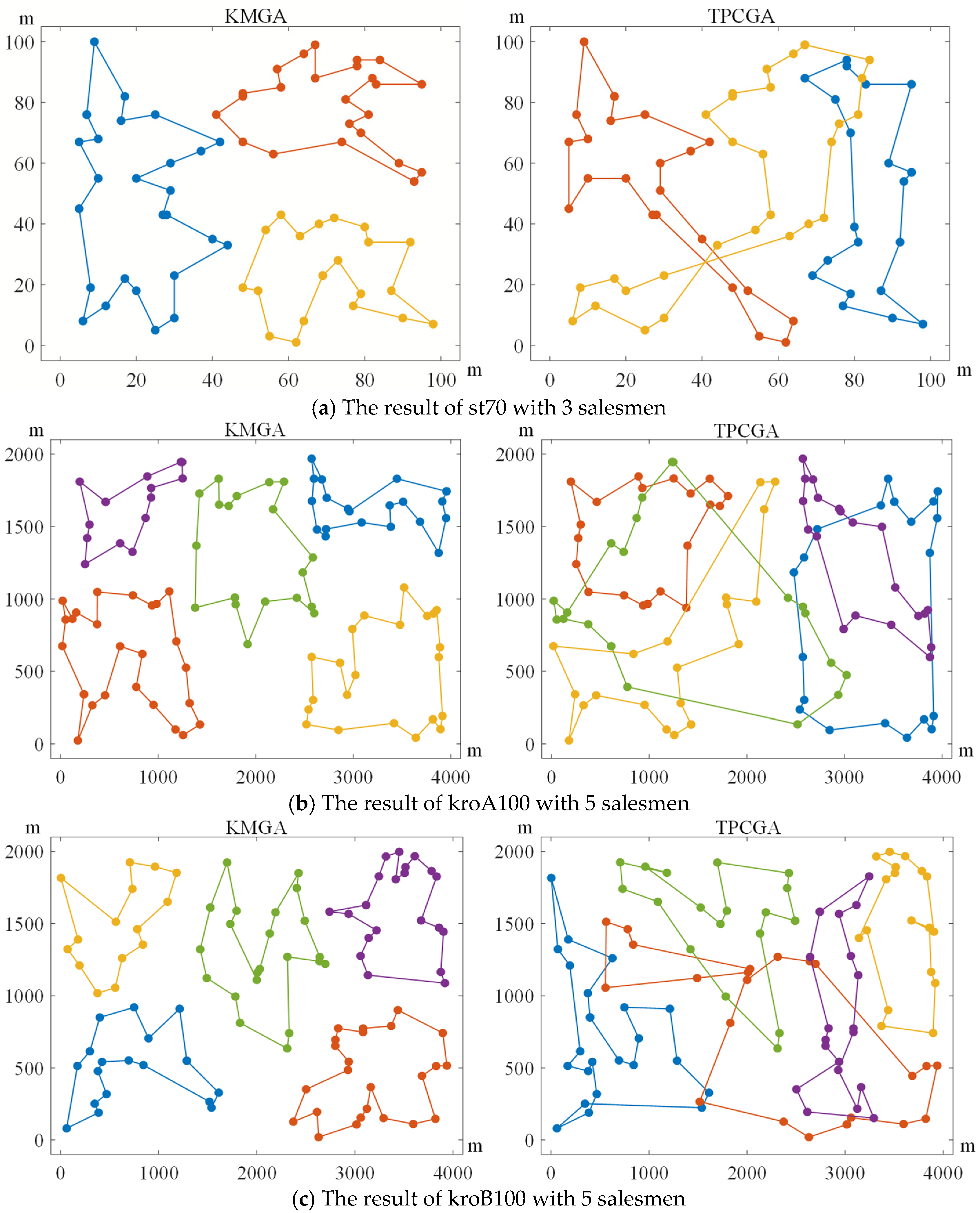
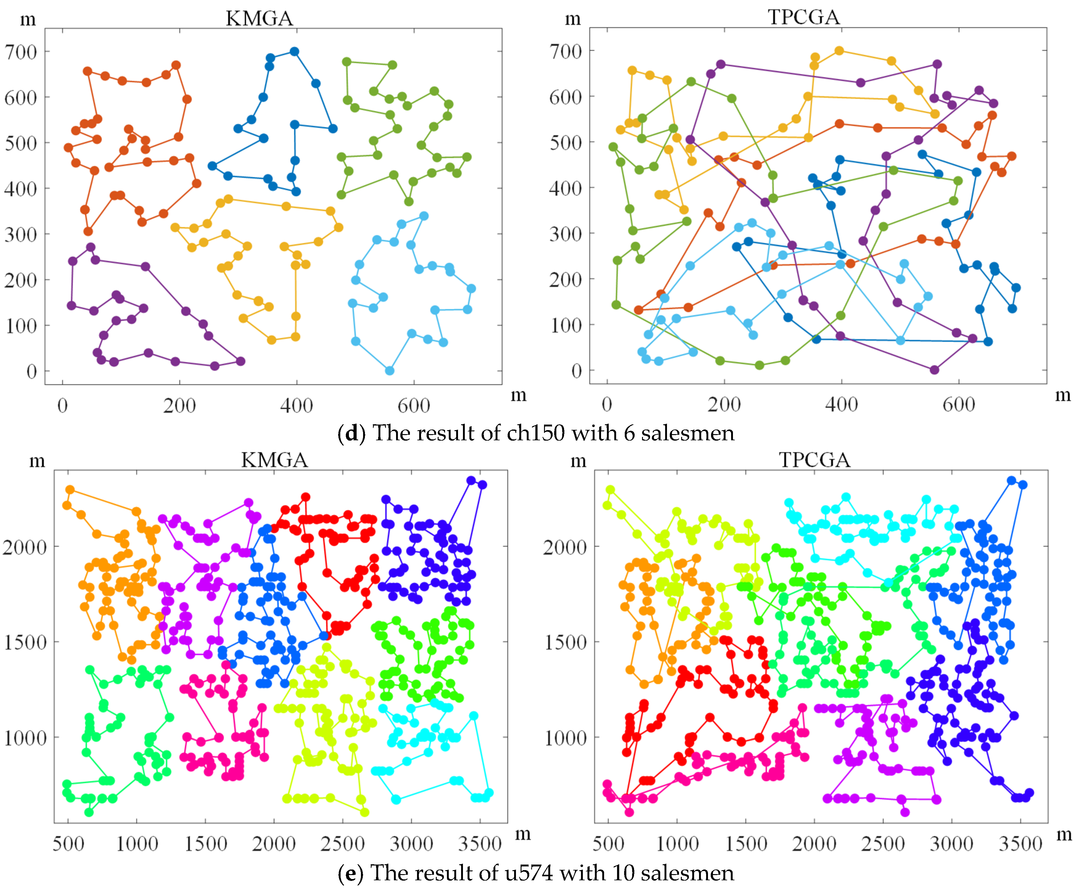
As visually demonstrated in the subfigures (a)–(e) of Figure 4, the proposed KMGA exhibits significantly improved spatial distribution characteristics in the solutions for the MTSP compared to those generated by the TPCGA. Specifically, the intersecting paths observed in the TPCGA-based solutions result from a fundamental misalignment between stochastic genetic operators and the geometric properties of Euclidean space. Conventional crossover and mutation operations fail to preserve the non-crossing condition inherent in optimal MTSP tours. In contrast, the regions assigned to each salesman under the KMGA show clear spatial segregation with non-overlapping paths. This characteristic is of considerable practical value in UAV inspection tasks, as it effectively reduces the risk of in-flight collisions caused by path intersections.

In order to quantify the KMGA’s advantage in avoiding the path crossover issues through the data, the minimum distances between paths are calculated to support the aforementioned claim in this paper. The results are shown in

Table 2. The average minimum distance between paths of the MTSP comparative simulations.

Instances	Algorithms	Avg Minimum Distance Between Paths/(m)
st70	TPCGA	0.0000
	proposed KMGA	4.7361
kroA100	TPCGA	0.0000
	proposed KMGA	176.0775
kroB100	TPCGA	0.0000
	proposed KMGA	169.2482
ch150	TPCGA	0.0000
	proposed KMGA	34.2482
u574	TPCGA	0.0000
	proposed KMGA	25.3728

. The results indicate that, due to path crossover issues in the paths planned by the TPCGA, the shortest distance between paths is 0. In contrast, the KMGA proposed in this paper avoids this problem by pre-partitioning the task area.

To quantitatively validate the superiority of the proposed algorithm,

Table 3. The data of the MTSP comparative simulations.

Instances	Algorithms	Avg Length/(m)	Std of Length/(m)	Avg Time/(s)	Std of Time/(s)
st70	TPCGA	782.4375	50.9492	5.0385	0.0414
	proposed KMGA	704.6701	1.9412	4.6021	0.3582
kroA100	TPCGA	31,951.8122	2234.0800	6.9428	0.2599
	proposed KMGA	22,596.9524	29.8465	6.7638	0.5185
kroB100	TPCGA	31,698.9087	2478.1988	6.9603	0.2139
	proposed KMGA	23,411.2550	47.4002	6.6826	0.3617
ch150	TPCGA	12,007.4536	572.2721	9.8412	0.3986
	proposed KMGA	6990.8464	23.7484	9.5706	0.6076
u574	TPCGA	44,886.1364	210.5891	49.2606	5.0860
	proposed KMGA	40,664.4786	211.9389	48.5646	3.1721

summarizes the statistical results from five simulation instances, each consisting of 20 independent trials. The performance of the two algorithms is compared in this paper by conducting appropriate statistical significance tests. Before evaluating the average performance of the two algorithms, it is necessary to evaluate the homogeneity of the variances by using Levene’s tests. Levene’s tests are firstly conducted on the variance of the path length, and the results are shown in

Table 4. The results of the Levene’s tests of the MTSP comparative simulations.

Instances	Levene Stat of Length	p Value of Length	Levene Stat of Time	p Value of Time
st70	52.9823	0.0000	23.6946	0.0000
kroA100	37.7687	0.0000	6.1574	0.0176
kroB100	35.6870	0.0000	6.2327	0.0170
ch150	29.5864	0.0000	0.2653	0.6095
u574	0.1127	0.7389	6.0579	0.0185

. The data indicates that, with the exception of the u574 group, the variances of the remaining groups do not satisfy the assumption of the homogeneity of variances (significance level is 0.05). Therefore, the Welch t-test is employed for the first four groups, while the standard t-tests are used for the last group. The results are shown in

Table 5. The results of the statistical significance tests of the MTSP comparative simulations.

Instances	t Stat of Length	p Value of Length	t Stat of Time	p Value of Time
st70	−7.4650	0.0000	−5.9303	0.0000
kroA100	−18.2506	0.0000	−1.3454	0.1893
kroB100	−14.5745	0.0000	−2.8801	0.0072
ch150	−38.1778	0.0000	−1.6230	0.1129
u574	−61.5910	0.0000	−0.5062	0.6162

. Similarly, the Levene’s tests are firstly employed for the variances in time, and the results are shown in Table 4. Based on the results of the Levene’s tests, the standard t-test is employed for the ch150 group, while the Welch t-tests are used for the remaining four groups. The results are also documented in Table 5.

The results of the statistical significance tests across the five benchmark instances demonstrate that the KMGA achieves statistically significant improvements in solution quality at a significance level of 0.05. Specifically, the average tour length and mean computation time obtained by the KMGA were reduced by 23.2373%. In terms of computational efficiency, the KMGA demonstrates superior performance over TPCGA in some instances, while in other instances, its performance is comparable to that of TPCGA.

5.2. The Simluations of the MNPP

5.2.1. The MNPP Simulations with Different Neighborhood Radius Values

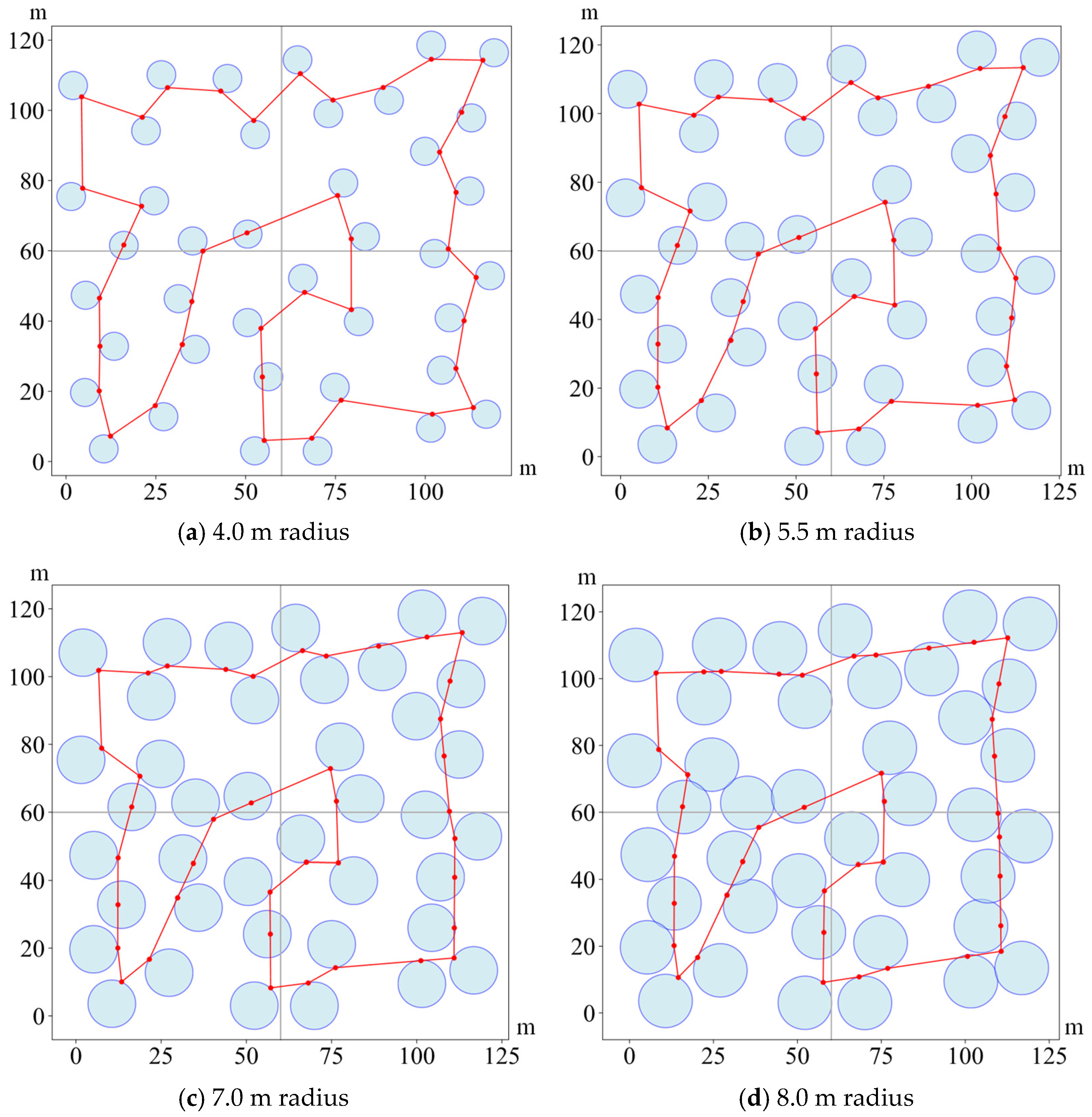
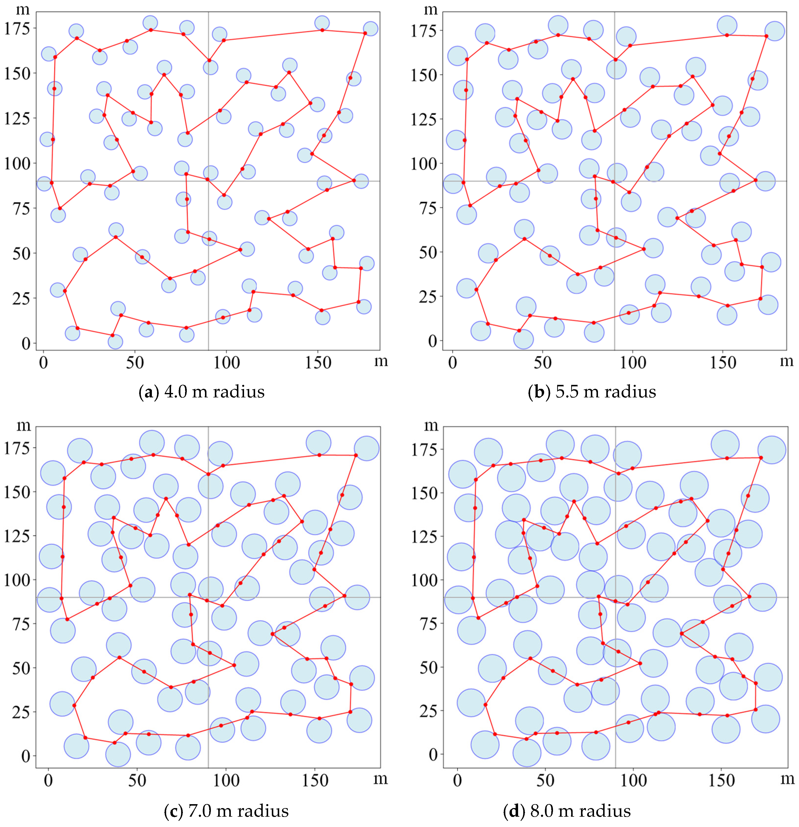
In order to conduct the sensitivity analysis on the assumption of the neighborhood radius and identify how the algorithm performance with the radius varies, four groups’ simulations of the MNPP with the neighborhood number values of 40 and 70 and the neighborhood radius values of 4.0 m, 5.5 m, 7.0 m, and 8.0 m are set. The distances between the nodes in the four groups are all set as 15.0 m, and the MNPP in the four groups is solved via the MNIDP.

The image results obtained from the solution are shown in Figure 5 and Figure 6. As shown in the figure, the paths tend to shorten as the neighborhood radius gradually increases. However, when the distance between the nodes is less than twice the neighborhood radius, overlapping neighborhoods occur. This results in multiple feasible path choices within the overlapping neighborhoods, making the scenario more complex. The MNIDP algorithm proposed in this paper cannot effectively resolve such overlapping neighborhood situations. Therefore, it assumes that the distance between any two nodes is no less than twice the neighborhood’s radius in this work.

To more clearly demonstrate the impact of neighborhood variations on the algorithm performance, the statistical data are summarized in

Table 6. The data of the MNPP simulations with different neighborhood radius values.

Instances	Radius/(m)	Avg Length/(m)	Std of Length/(m)	Avg Time/(s)	Std of Time/(s)
40 neighborhoods	4.0	610.9333	0.0743	6.8520	0.0868
	5.5	567.8601	0.1397	6.2867	0.0743
	7.0	533.2458	0.1316	5.4650	0.1126
	8.0	514.9898	0.3989	4.7537	0.1416
70 neighborhoods	4.0	1270.3026	0.1187	11.6093	0.0836
	5.5	1190.1203	0.2427	10.2489	0.2192
	7.0	1120.8434	0.2144	9.6732	0.2013
	8.0	1080.9589	0.2503	8.7461	0.0784

. As shown in Table 6, both the computation time and the calculated path length of the algorithm gradually decrease as the neighborhood radius increases. Then, a statistical significance test is performed on the data. The basic steps are similar to the steps in Section 5.1. The test methods employed in this section are Levene’s tests and an analysis of variance (ANOVA)/Welch ANOVA, and the results are shown in

Table 7. The results of the Levene’s tests of the MNPP simulations with different neighborhood radius values.

Instances	Levene Stat of Length	p Value of Length	Levene Stat of Time	p Value of Length
40 neighborhoods	1.4234	0.2456	0.5804	0.6303
70 neighborhoods	1.9191	0.1369	3.8043	0.0149

and

Table 8. The results of the ANOVA/Welch ANOVA of the MNPP simulations with different neighborhood radius values.

Instances	f Stat of Length	p Value of Length	f Stat of Time	p Value of Length
40 neighborhoods	496,124.8202	0.0000	1037.7262	0.0000
70 neighborhoods	2,130,763.2091	0.0000	2805.3236	0.0000

. The results of the statistical significance test further corroborate the previously discussed conclusion regarding the relationship between algorithm performance and neighborhood radius.

5.2.2. The Comparative Simulations of the MNPP

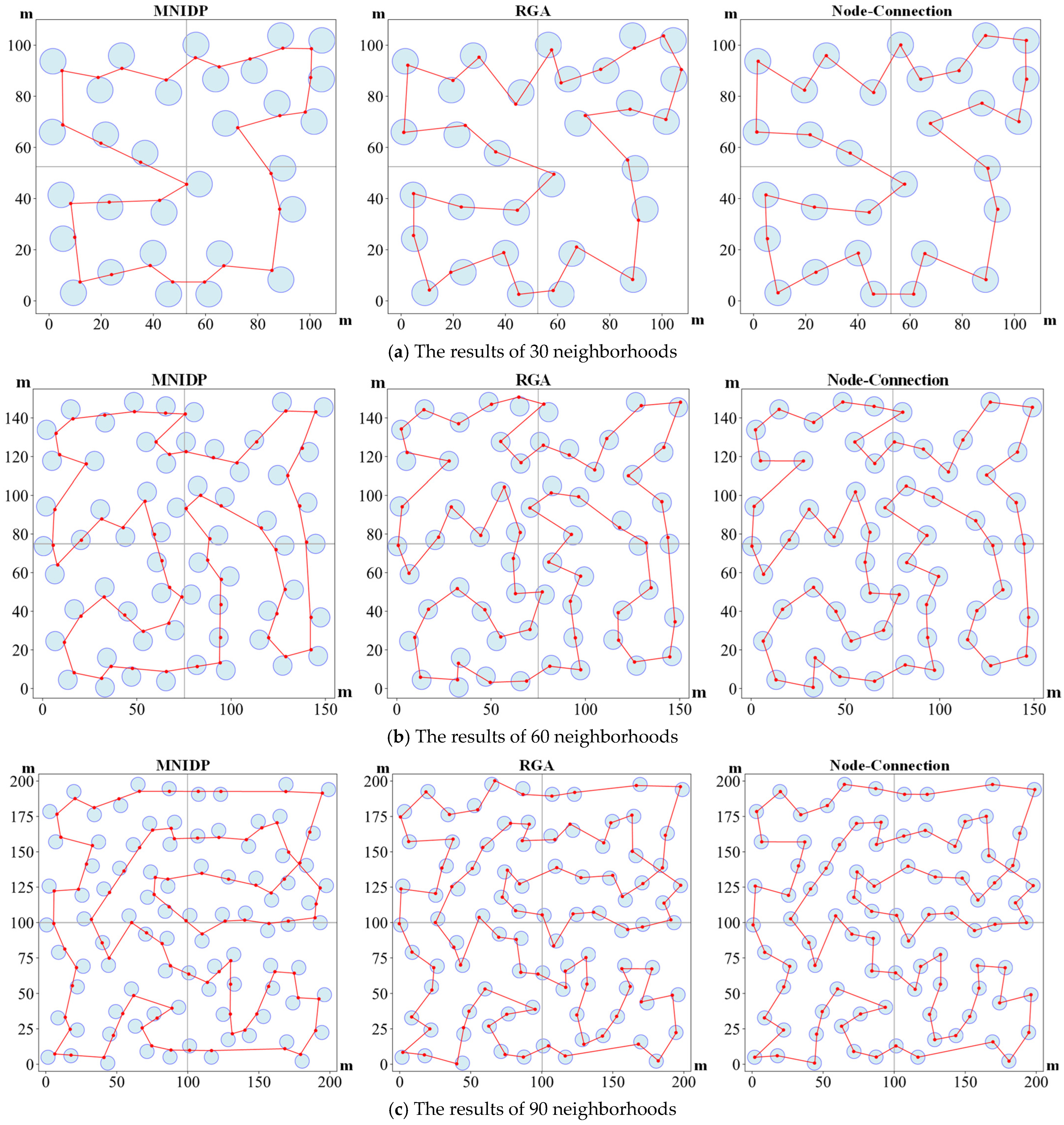
The performance evaluation of the MNIDP on the MNPP is presented in this sub-Section. The simulation environments are configured with 30, 60, and 90 neighborhoods, respectively, and the RGA and node-connection method (a baseline approach that directly connects the nodes) are selected as the baseline algorithms for comparison. The simulation results are shown in Figure 7, the simulation data are shown in

Table 9. The data of the MNPP comparative simulations.

Instances	Approaches	Average Path Length/(m)	Standard Deviation of Path Length/(m)
30 neighborhoods	Node-Connection	571.7623	4.3812
	RGA	556.5171	6.2885
	Proposed MNIDP	429.0575	2.9024
60 neighborhoods	Node-Connection	1196.5320	13.9907
	RGA	1178.2461	14.4318
	Proposed MNIDP	931.0527	15.7290
90 neighborhoods	Node-Connection	1892.9093	15.3603
	RGA	1880.4838	19.6851
	Proposed MNIDP	1537.5530	17.8415

, and the results of the statistical significance tests for the data are placed in

Table 10. The results of the statistical significance tests of the MNPP comparative simulations.

Instances	Levene Stat	p Value of Levene	f Stat	p Value of ANOVA
30 neighborhoods	5.7546	0.0053	8319.7989	0.0000
60 neighborhoods	0.1951	0.8233	1923.8444	0.0000
90 neighborhoods	0.4061	0.6682	2461.6840	0.0000

.

As shown in the three subfigures of Figure 7, the path planned by the MNIDP exhibits fewer kinks and closer distances between the path nodes compared to the other two baseline methods. This result is corroborated by the data in Table 9; it shows that the average path length planned by the MNIDP is over 20% shorter than the path length of the other two methods. To further enhance the reliability of the conclusion, statistical significance tests are conducted on the simulation data, following the same procedure and methodology as in Section 5.2.1. The results of the statistical significance tests further demonstrate that the MNIDP algorithm proposed in this paper exhibits a superior performance compared to the other two methods.

5.3. The Comparative Simulations of the MTSPN

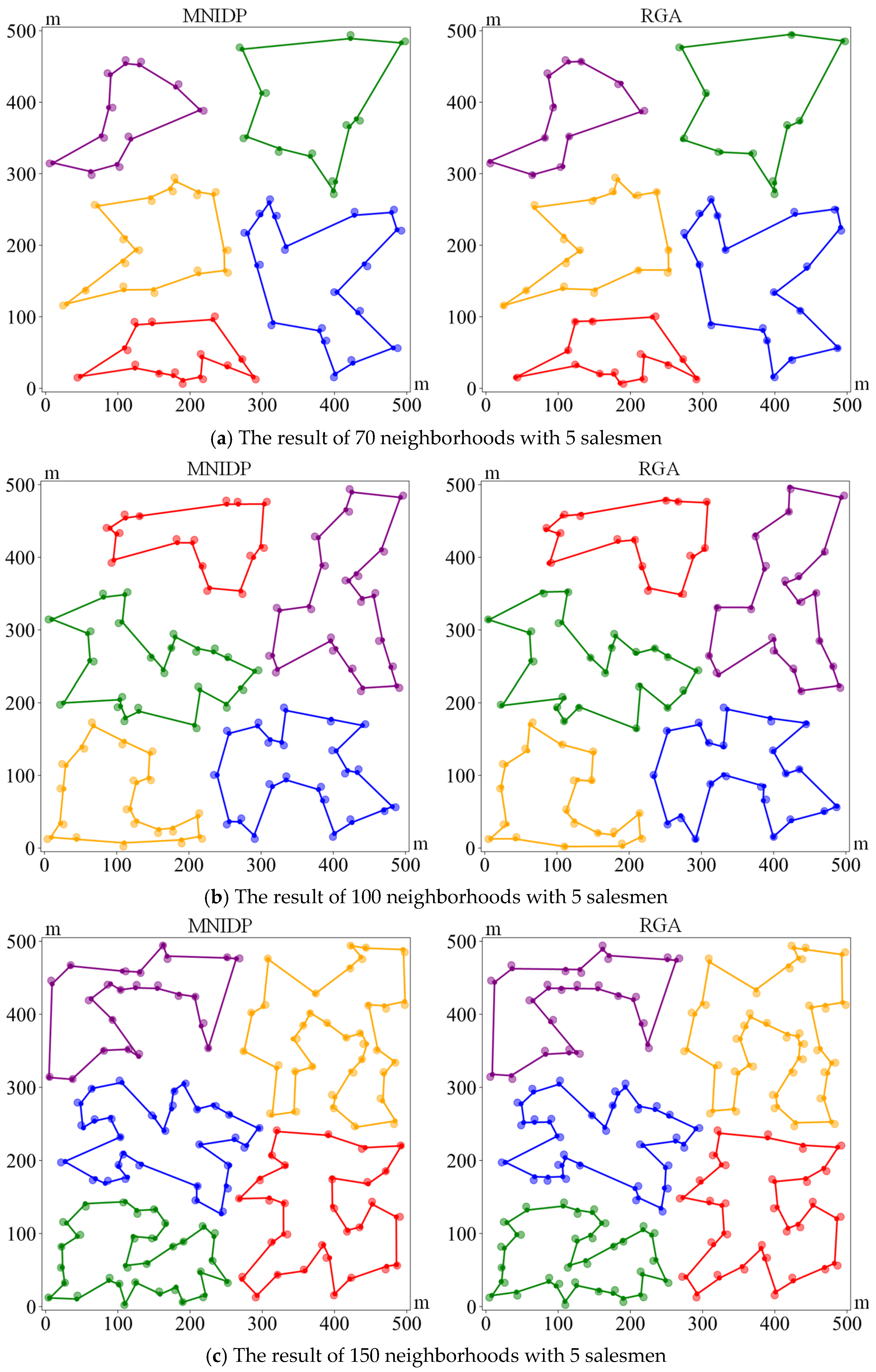
For the comparative simulations, 70, 100, and 150 neighborhoods with five salesmen will be, respectively, generated as examples.

To mitigate the effects of stochastic variations in the simulations, 20 independent runs were conducted for each instance. The final average path length for each configuration is documented in

Table 11. The data of the MTSPN comparative simulations.

Instances	Approaches	Average Path Length/(m)	Standard Deviation of Path Length/(m)
70 neighborhoods	Node-Connection	3749.1103	0.3126
	RGA	3687.4058	11.8996
	Proposed MNIDP	3449.0536	4.7858
100 neighborhoods	Node-Connection	4453.0670	20.9587
	RGA	4376.8528	28.1452
	Proposed MNIDP	3989.5648	22.4328
150 neighborhoods	Node-Connection	5594.3614	19.4487
	RGA	5512.0835	17.2291
	Proposed MNIDP	4956.2008	21.5898

, and the results of the three instances are shown in Figure 8.

A comparative analysis of the three subplots in Figure 8 indicates that the proposed MNIDP exhibits consistent and significant advantages in path-point selection over the RGA. Simulation results demonstrate that the path points selected by the MNIDP closely align with the two typical patterns of the shortest path node distribution derived theoretically in the previous section. These findings further validate the effectiveness of the MNIDP in adhering to the shortest path criterion for path optimization problems.

Furthermore, the results presented in Table 11 indicate that, across the three simulation instances, the MNIDP achieves reductions in the path length of 8.00%, 10.41%, and 11.41%, respectively, compared to the node-connection method. Similarly, relative to the RGA, the MNIDP yields path length reductions of 6.46%, 8.85%, and 10.08% for the same instances. To further illustrate the advantages of the MNIDP algorithm, the statistical significance tests are conducted in this paper. The basic workflow is similar to the workflow in Section 5.1, and the test method is changed from the t-tests to ANOVA and Welch ANOVA. The results are shown in

Table 12. The results of the statistical significance tests of the MTSPN comparative simulations.

Instances	Levene Stat	p Value of Levene	f Stat	p Value of ANOVA
70 neighborhoods	8.3543	0.0007	36,474.7105	0.0000
100 neighborhoods	0.3862	0.6814	2029.8185	0.0000
150 neighborhoods	0.8182	0.8182	6018.7891	0.0000

. The results of the statistical significance tests demonstrate that the MNIDP algorithm proposed in this paper exhibits greater statistical superiority compared to the other two methods.

These results collectively demonstrate that the proposed MNIDP algorithm not only validates its theoretical foundation but also exhibits significant performance advantages over existing methods in solving the MNPP.

6. Conclusions

This paper proposes a composite task planning strategy integrating the KMGA and the MNIDP to address the multi-region multi-UAV cooperative task planning and optimization problem in UAV inspection scenarios. To simplify the solution process, the target problem is formulated as an MTSPN, and the MTSPN is decomposed into two subproblems: the MTSP and the MNPP. In order to solve the MTSP, the strategy first utilizes the KMGA to partition the MTSP into m TSPs to obtain the approximate optimal visiting sequences for the nodes of each TSP. Subsequently, based on the visiting sequences, the strategy utilizes the MNIDP to plan the paths between the corresponding neighborhoods of each node for the solution of the MNPP, from which an approximate optimal solution of the MTSPN can be obtained. Comprehensive comparative simulations between the proposed algorithms and a set of baseline methods demonstrate that the combined strategy exhibits significant performance advantages in solving the MTSPN. This work provides both theoretical underpinnings and a technical framework for cooperative UAV inspection mission planning.

Future work will focus on addressing the following unresolved challenges:

(1)

The swarm of UAVs sometimes comprise heterogeneous UAVs and the task allocation for such swarms must incorporate this heterogeneity as a consideration to ensure feasible mission execution. However, the homogeneity assumption of the MTSPN fails to accommodate this scenario. Therefore, efficiently solving the unbalanced and dynamic cooperative assignment between multiple UAVs and multiple regions is a challenge that needs further exploration [33].

(2)

The improvements of the KMGA will be made by optimizing the K-Means++ clustering criteria and introducing load balancing constraints into the clustering objective function. This approach achieves the goal of ensuring that the task loads among drones are essentially equal.

(3)

The KMGA and MNIDP algorithm proposed in this paper will be deployed on physical UAVs, and the effectiveness and performance of the algorithms will be demonstrated through physical experiments.

References

1. Li, C.; Liu, J.; Shen, X.; Liu, Z.; Gao, Y.; Leon, J.I. Multi-Objective Energy Management Strategy for Distribution Network With Distributed Renewable Based on Learning-Driven Model Predictive Control. IEEE Trans. Smart Grid 2025, 16, 4968–4982. [Google Scholar] [CrossRef]
2. Shen, X.; Liu, G.; Liu, J.; Gao, Y.; Leon, J.I. Fixed-Time Sliding Mode Control for NPC Converters With Improved Disturbance Rejection Performance. IEEE Trans. Ind. Inform. 2025, 21, 4476–4487. [Google Scholar] [CrossRef]
3. Shen, X.; Liu, J.; Liu, G.; Zhang, J.; Leon, J.I.; Wu, L.; Franquelo, L.G. Finite-Time Sliding Mode Control for NPC Converters With Enhanced Disturbance Compensation. IEEE Trans. Circuits Syst. I Regul. Pap. 2025, 72, 1822–1831. [Google Scholar] [CrossRef]
4. Bakirci, M. Enhancing air pollution mapping with autonomous UAV networks for extended coverage and consistency. Atmos. Res. 2024, 306, 107480. [Google Scholar] [CrossRef]
5. Ma, W.; Guo, X. Prescribed-Time Cooperative Guidance Law for Multi-UAV with Intermittent Communication. Drones 2024, 8, 748. [Google Scholar] [CrossRef]
6. He, C.; Ouyang, H.; Huang, W.; Li, S.; Zhang, C.; Ding, W.; Zhan, Z. An adaptive heuristic algorithm with a collaborative search framework for multi-UAV inspection planning. Appl. Soft Comput. 2025, 174, 112969. [Google Scholar] [CrossRef]
7. Rusell, R.A. Technical Note—An Effective Heuristic for the M-Tour Traveling Salesman Problem with Some Side Conditions. Oper. Res. 1977, 25, 517–524. [Google Scholar] [CrossRef]
8. Zatout, M.S.; Rezoug, A.; Rezoug, A.; Baizid, K.; Iqbal, J. Optimisation of fuzzy logic quadrotor attitude controller—Particle swarm, cuckoo search and BAT algorithms. Int. J. Syst. Sci. 2021, 53, 883–908. [Google Scholar] [CrossRef]
9. Pan, J.; Wang, D. An Ant Colony Optimization Algorithm for Multiple Travelling Salesman Problem. In Proceedings of the First International Conference on Innovative Computing, Information and Control-Volume I (ICICIC’06), Beijing, China, 30 August–1 September 2006; pp. 210–213. [Google Scholar] [CrossRef]
10. Carter, A.E.; Ragsdale, C.T. A new approach to solving the multiple traveling salesperson problem using genetic algorithms. Eur. J. Oper. Res. 2006, 175, 246–257. [Google Scholar] [CrossRef]
11. Zhang, Y.; Han, X.; Dong, Y.; Xie, J.; Xie, G.; Xu, X. A novel state transition simulated annealing algorithm for the multiple traveling salesmen problem. J. Supercomput. 2021, 77, 11827–11852. [Google Scholar] [CrossRef]
12. Chen, Y.; Jia, Z.; Ai, X.; Yang, D.; Yu, J. A modified two-part wolf pack search algorithm for the multiple traveling salesmen problem. Appl. Soft Comput. 2017, 61, 714–726. [Google Scholar] [CrossRef]
13. Hu, S.; Lu, H.; Xiang, L.; Shen, Q. Fuzzy C-means Clustering Based Partheno-genetic Algorithm for Solving MMTSP. Comput. Sci. 2020, 47, 219–223. [Google Scholar] [CrossRef]
14. Modares, A.; Somhom, S.; Enkawa, T. A self-organizing neural network approach for multiple traveling salesman and vehicle routing problems. Int. Trans. Oper. Res. 1999, 6, 591–606. [Google Scholar] [CrossRef]
15. Qu, H.; Yi, Z.; Tang, H. A columnar competitive model for solving multi-traveling salesman problem. Chaos Solitons Fractals 2007, 31, 1009–1019. [Google Scholar] [CrossRef]
16. Wacholder, E.; Han, J.; Mann, R.C. A neural network algorithm for the multiple traveling salesmen problem. Biol. Cybern. 1989, 61, 11–19. [Google Scholar] [CrossRef]
17. Hsu, C.; Tsai, M.; Chen, W. A study of feature-mapped approach to the multiple travelling salesmen problem. IEEE Int. Symp. Circuits Syst. 1991, 3, 1589–1592. [Google Scholar] [CrossRef]
18. Razzaq, S.; Xydeas, C.; Mahmood, A.; Ahmed, S.; Ratyal, N.I.; Iqbal, J. Efficient optimization techniques for resource allocation in UAVs mission framework. PLoS ONE 2023, 18, e0283923. [Google Scholar] [CrossRef]
19. Chen, Z.; Sun, C.; Shao, X.; Zhao, W. A descent method for the Dubins traveling salesman problem with neighborhoods. Front. Inf. Technol. Electron. Eng. 2021, 22, 732–740. [Google Scholar] [CrossRef]
20. Liu, S.; Lin, Z.; Huang, W.; Yan, B. Technical development and future prospects of cooperative terminal guidance based on knowledge graph analysis: A review. J. Zhejiang Univ. Sci. A 2025, 26, 605–634. [Google Scholar] [CrossRef]
21. Gentilini, I.; Margot, F.; Shimada, K. The travelling salesman problem with neighbourhoods: MINLP solution. Optim. Methods Softw. 2013, 28, 364–378. [Google Scholar] [CrossRef]
22. Vicencio, K.; Davis, B.; Gentilini, I. Multi-goal path planning based on the generalized Traveling Salesman Problem with neighborhoods. In Proceedings of the 2014 IEEE/RSJ International Conference on Intelligent Robots and Systems, Chicago, IL, USA, 14–18 September 2014; pp. 2985–2990. [Google Scholar] [CrossRef]
23. Deckerová, J.; Váňa, P.; Faigl, J. Combinatorial lower bounds for the Generalized Traveling Salesman Problem with Neighborhoods. Expert Syst. Appl. 2024, 258, 125185. [Google Scholar] [CrossRef]
24. Xin, B.; Chen, J.; Xu, D.; Chen, Y. Hybrid encoding based differential evolution algorithms for Dubins traveling salesman problem with neighborhood. Control. Theory Appl. 2014, 31, 941–954. [Google Scholar]
25. Obermeyer, K. Path planning for a UAV performing reconnaissance of static ground targets in terrain. In Proceedings of the AIAA Guidance, Navigation, and Control Conference, Chigaco, IL, USA, 10–13 August 2009. [Google Scholar] [CrossRef]
26. Obermeyer, K.; Oberlin, P.; Darbha, S. Sampling-based roadmap methods for a visual reconnaissance UAV*. In Proceedings of the AIAA Guidance, Navigation, and Control Conference, Toronto, ON, Canada, 2–5 August 2010. [Google Scholar] [CrossRef]
27. Yu, X.; Hung, J.Y. Optimal path planning for an autonomous robot-trailer system. In Proceedings of the IECON 2012-38th Annual Conference on IEEE Industrial Electronics Society, Montreal, QC, Canada, 25–28 October 2012; pp. 2762–2767. [Google Scholar] [CrossRef]
28. Gao, C.; Wei, N.; Walteros, J.L. An Exact Approach for Solving Pickup-and-Delivery Traveling Salesman Problems with Neighborhoods. Transp. Sci. 2023, 57, 1560–1580. [Google Scholar] [CrossRef]
29. Clark, A. A Submodular Optimization Approach to the Metric Traveling Salesman Problem with Neighborhoods. In Proceedings of the 2019 IEEE 58th Conference on Decision and Control (CDC), Nice, France, 11–13 December 2019; pp. 3383–3390. [Google Scholar] [CrossRef]
30. Rathinam, S.; Sengupta, R.; Darbha, S. A Resource Allocation Algorithm for Multivehicle Systems with Nonholonomic Constraints. IEEE Trans. Autom. Sci. Eng. 2007, 4, 98–104. [Google Scholar] [CrossRef]
31. Puerto, J.; Valverde, C. The Hampered Travelling Salesman problem with Neighborhoods. Comput. Ind. Eng. 2024, 188, 109889. [Google Scholar] [CrossRef]
32. Wan, M.; Zhao, D.; Zhao, B. Combining Max pooling-Laplacian theory and k-means clustering for novel camouflage pattern design. Front. Neurorobot. 2022, 16, 1041101. [Google Scholar] [CrossRef]
33. Wang, W.; Lv, M.; Ru, L.; Lu, B.; Hu, S.; Chang, X. Multi-UAV Unbalanced Targets Coordinated Dynamic Task Allocation in Phases. Aerospace 2022, 9, 491. [Google Scholar] [CrossRef]
Figure 1. The two cases of path node existence, (a) case (a), (b) case (b).
Drones 09 00762 g001
Figure 2. The proof figures of two cases, (a) case (a), (b) case (b).
Drones 09 00762 g002
Figure 3. The sampling methods of two cases, (a) case (a), (b) case (b).
Drones 09 00762 g003
Figure 4. The results of the MTSP comparative simulation. In each subfigure, the left graph presents the result of the KMGA with the right graph illustrating the result of the TPCGA. In each subfigure, the points of different colors represent the nodes that require inspection by different UAVs, and the node inspection sequence is obtained by connecting these points with lines. In all subfigures, the points and lines of different colors represent the inspection nodes and paths of different traveling salesmen, respectively.
Drones 09 00762 g004aDrones 09 00762 g004b
Figure 5. The results of the MNPP with 40 neighborhoods and a different radius.
Drones 09 00762 g005
Figure 6. The results of the MNPP with 70 neighborhoods and a different radius.
Drones 09 00762 g006
Figure 7. The results of the MNPP comparative simulation. In each subfigure, the left graph represents the results planned by the MNIDP, the middle graph represents the results planned by the RGA, and the right graph represents the results of node connection.
Drones 09 00762 g007
Figure 8. The results of the MTSPN comparative simulation. In each subfigure, the left graph presents the result of the MNIDP with the right graph illustrating the result of the RGA. Both algorithms select a path node based on the node sequence planned by KMGA and subsequently visit the neighborhoods. In all subfigures, the points and lines of different colors represent the inspection nodes and paths of different traveling salesmen, respectively.
Drones 09 00762 g008