Feature-Generation-Replay Continual Learning Combined with Mixture-of-Experts for Data-Driven Autonomous Guidance

Highlights

What are the main findings?

• Propose a continual learning method combining feature-generation replay with MoE-LoRA to alleviate catastrophic forgetting for UGV autonomous guidance.
• Design a structure-enhanced feature generation method to improve alignment of generated and real features.

What is the implication of the main finding?

• Solve catastrophic forgetting in UGV autonomous guidance under dynamic domain changes.
• Meet resource constraints of UGV on-board edge devices for practical deployment.

Abstract

Continual learning (CL) is a key technology for enabling data-driven autonomous guidance systems to operate stably and persistently in complex and dynamic environments. Its core goal is to enable the model to continuously learn new scenarios and tasks after deployment, without forgetting existing knowledge, and finally achieving stable decision-making in the different scenarios over a long period. This paper proposes a continual learning method that combines feature-generation-replay with Mixture-of-Experts and Low-Rank Adaptation (MoE-LoRA). This method retains the key features of historical tasks by feature repla and realizes the adaptive selection of old and new knowledge by the Mixture-of-Experts (MoE), which alleviates the conflict between knowledge while ensuring learning efficiency. In the comparison experiments, we compared the proposed method with the representative continual learning methods, and the experimental results show that our method outperforms the representative continual learning methods, and the ablation experiments further demonstrate the role of each component. This work provides technical support for the long-term maintenance and new task expansion of data-driven autonomous guidance systems, laying a foundation for their stable operation in complex, variable real-world scenarios.

1. Introduction

In scenarios of autonomous navigation and large-scale operations for Unmanned Ground Vehicles (UGVs), the insufficient generalization capability of end-to-end models in unknown environments has become a core bottleneck that restricts the implementation of their autonomy, drives up deployment costs, and amplifies operational risks [1,2]. From the perspective of the spatial dimension of UGVs’ actual operations, such unknown environments can be systematically decomposed into two deeply coupled layers, which together form a full-chain generalization barrier spanning from macroscopic scenario adaptation to microscopic operational decision-making, directly impacting the autonomous operation logic of UGVs:

Firstly, the cross-domain heterogeneity of geographical scenarios covers the main operational areas of UGVs, including urban structured roads, narrow rural roads, and mountainous outdoor roads [3]. There are significant differences in environmental rules and infrastructure between different scenarios—while urban scenarios feature clear lane lines, traffic light systems, and pedestrian right-of-way norms, mountainous scenarios are dominated by temporary rolled paths and lack lane markers. This discrepancy causes a sharp shift in the data distribution collected by sensors (such as camera and LiDAR) mounted on UGVs, directly undermining the consistency of their autonomous perception. For instance, models trained in urban environments struggle to identify the boundaries of unstructured paths in mountainous areas, and vice versa. Consequently, the difficulty of model deployment is greatly increased: if models are trained separately for different scenarios, repeated data annotation and parameter debugging are required, making it impossible to achieve the efficient application goal of “one deployment for multi-scenario adaptation”.

Secondly, the structural complexity of road network topology is reflected in the differences in geometric parameters across various scenarios, such as road network forms like urban roundabouts, rural T-junctions, and continuous sharp bends in mountainous areas. Such differences directly pose challenges to the operational and planning capabilities of UGVs: the small-curvature characteristic of continuous sharp bends in mountains requires the UGV’s path planning algorithm to simultaneously complete coordinated decisions on speed adjustment, steering prediction, and obstacle avoidance within a short period. If traditional end-to-end models do not cover such topological features, they are prone to operational errors like stuck path planning and excessive steering and may even lead to rollover risks; the multi-entry interleaving characteristic of urban roundabouts, on the other hand, tests the UGV’s ability to independently judge dynamic traffic flow. When the model’s generalization capability is insufficient, operational issues such as “hesitation to enter the roundabout” or “collision due to rushing” may occur [4].

The two layers mentioned above are deeply coupled—the heterogeneity of geographical scenarios exacerbates the difficulty in perceiving road network topology. For example, vegetation cover in mountainous scenarios may obscure the entrances of branch roads; meanwhile, the complexity of road network topology amplifies the decision-making pressure caused by differences in environmental rules. For instance, on unmarked rural branch roads, UGVs need to independently determine the direction of travel instead of relying on preset traffic rules. To address the significant issues arising from distribution differences, we have conducted research on domain-incremental learning (DIL) for autonomous guidance, with a focus on enabling the guidance model to continuously maintain good generalization performance across multiple environments with large distribution differences, without suffering from catastrophic forgetting.

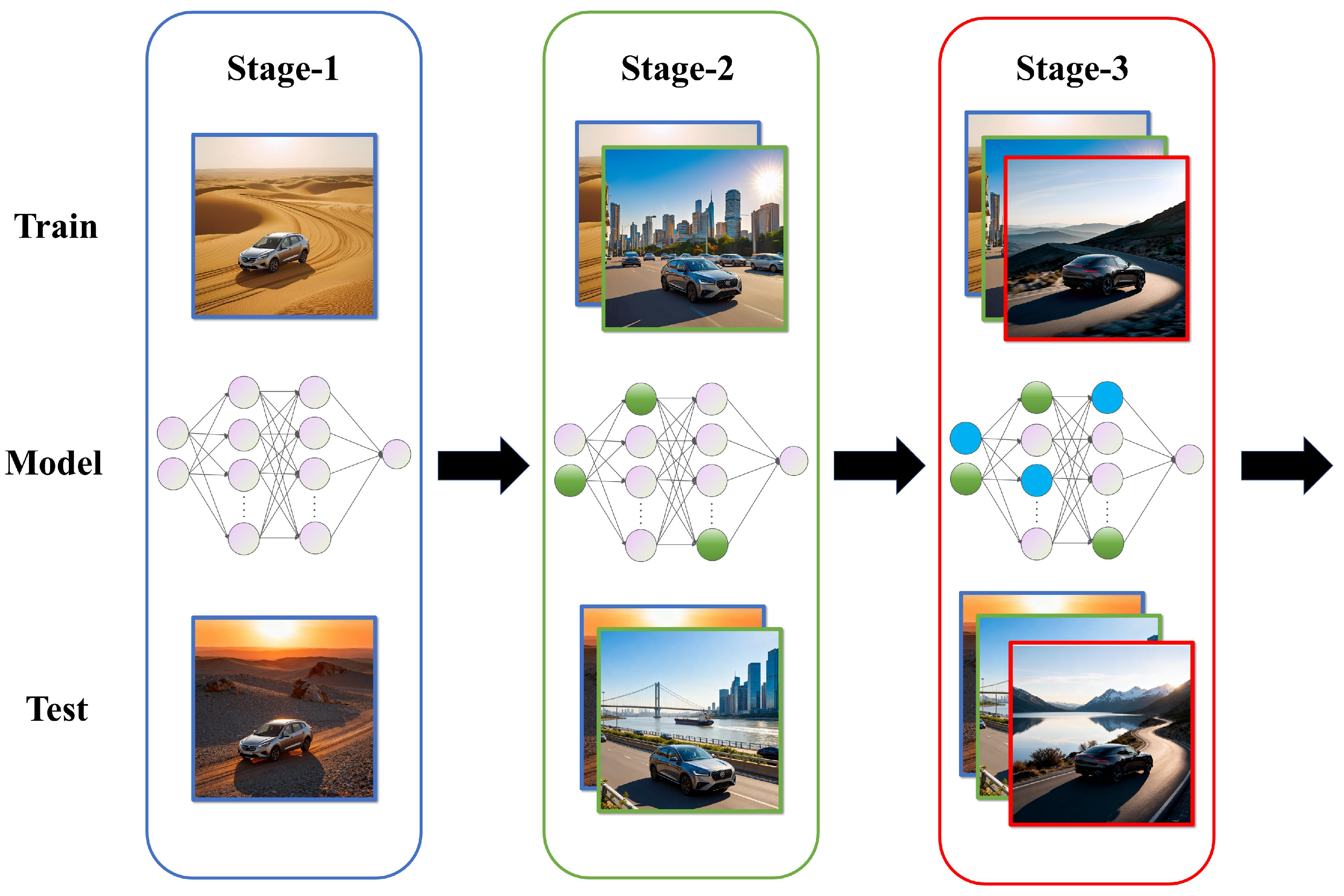
Figure 1 illustrates an example of DIL for autonomous guidance. Each stage requires the model to learn from the new distribution while also needing to retain as much as possible the knowledge learned in previous stages. For example, the model is trained on data featuring a desert scene and then tested on data in the same scenario. Moving to Stage-2, the model learns from new data showing urban scenarios (with cars in a city environment) while needing to retain knowledge from Stage-1. In Stage-3, the model continues to learn from data with yet another distinct scenario distribution, all the while striving to preserve the knowledge acquired from both Stage-1 and Stage-2. Each stage represents a notable shift in the data’s domain distribution, demanding the model adapt to the new data and maintain previously learned information.

Most of the existing research on continual learning focuses on class-incremental learning and task-incremental learning and lacks continuous learning designs tailored to specific domains. First, existing methods are mainly developed for general tasks and do not take into account the unique characteristics of autonomous guidance. For instance, replay-based methods require the storage of large amounts of raw sensor data (such as LiDAR point clouds), which is impractical for resource-constrained edge devices in autonomous vehicles. Although feature-generation-replay methods have high storage efficiency, they lack customized designs for the sparse and high-dimensional environmental features in guidance tasks. Second, the integration of MoE and Low-Rank Adaptation (LoRA) in continual learning has not been fully explored: existing MoE-LoRA research only focuses on single-task fine-tuning and cannot adapt to the continuous domain changes in autonomous guidance. Finally, the reproduction quality of generated features is poor: generative replay relies on synthetic features to replace original historical data, but the loss of traditional Generative Adversarial Networks (GANs) only matches the overall data distribution while ignoring the sparse patterns and statistical features of LiDAR features.

To fill these gaps, we proposed a continual learning method that combines with Mixture-of-Experts for autonomous guidance. This work makes the following contributions:

• We propose an continual learning method based on feature-generation replay for autonomous guidance models of UGVs, which effectively addresses the effectiveness and robustness of such models in cross-domain distributed scenarios.
• We design a feature generator based on structural loss for LiDAR point clouds, which can generate data of historical scenarios in autonomous guidance, thereby reducing forgetting during the training process of unmanned vehicle autonomous guidance models and improving the models’ adaptability to environments.
• We develop a dynamic expansion structure based on MoE-LoRA, which can perform knowledge expansion for unmanned vehicle autonomous guidance models and further enhance the models’ environmental adaptability.

2. Background

This section focuses on three core aspects closely aligned with the research scope of this paper: data-driven autonomous guidance tasks, domain incremental learning, and the MoE model.

First, the data-driven autonomous guidance task is the primary problem targeted by this research. As a comprehensive task integrating the perception module, positioning module, and trajectory prediction module, this section will elaborate on its definition, basic composition, and key challenges, laying a foundational understanding for the subsequent research discussion. Second, continual learning constitutes the core issue addressed in this study. We will first clarify the definition of continual learning and summarize its current research status, then provide a detailed exposition of domain incremental learning—a subfield of continual learning that is the focus of this paper—to highlight its relevance to our research objectives. Finally, the MoE model is the key method adopted for model construction in this paper. This section will review the current research progress of the MoE model and further discuss the specific purposes and academic significance of introducing this model into our research framework, demonstrating its rationality and innovation in addressing the studied problems.

2.1. Data-Driven Autonomous Guidance of UGVs

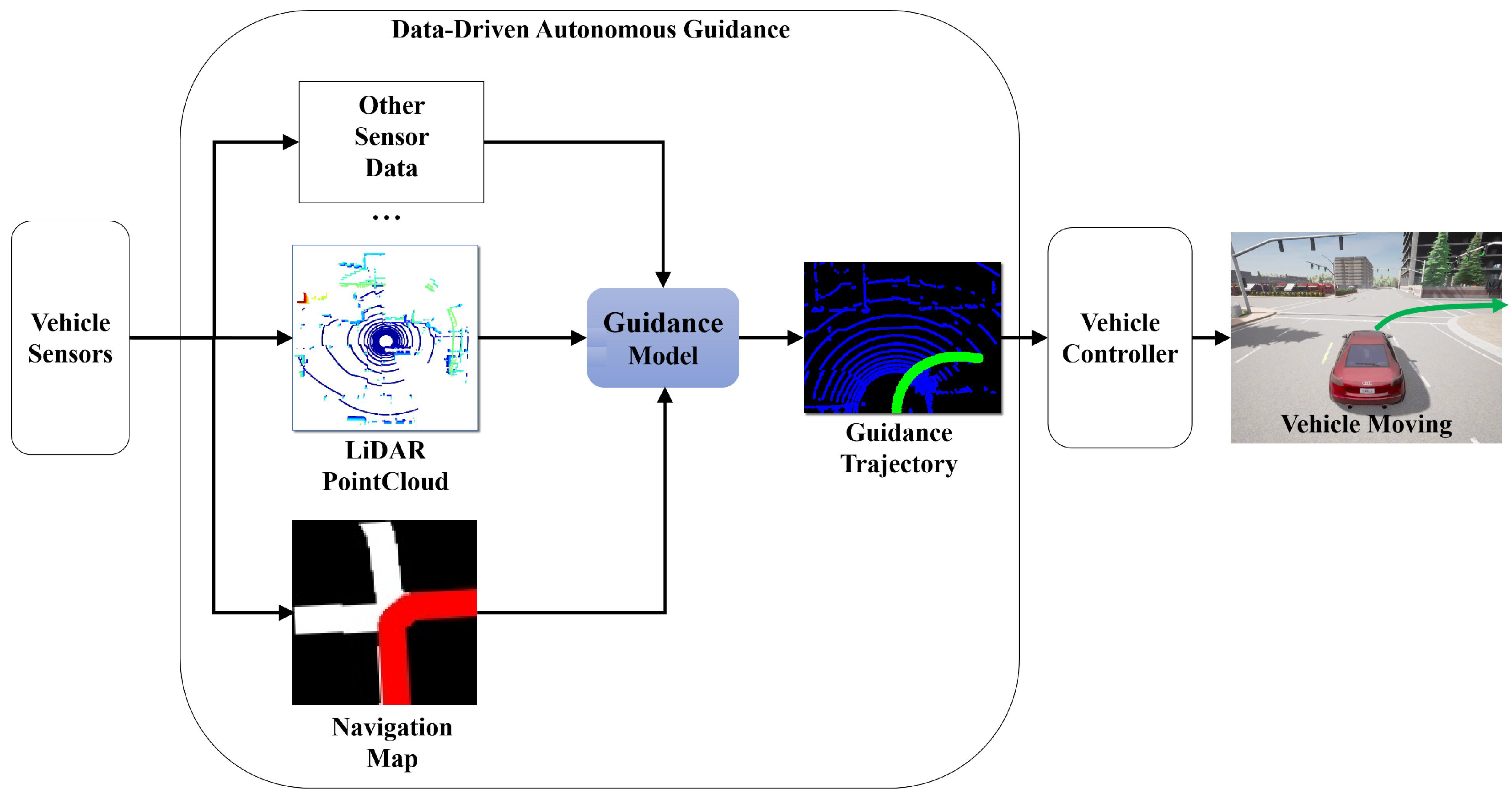
In our previous work [5], we studied the problem of fusing based on existing models to obtain a more robust guidance model and verified the workflow of the data-driven autonomous guidance method. The workflow of the data-driven autonomous guidance system is shown in Figure 2. The core is to generate the guidance trajectory to provide steering guidance and without dependence on high-precision positioning. The objective is to establish a direct mapping from environmental information (such as LiDAR point cloud, navigation map, etc.) to the local guidance trajectory of the vehicle, avoiding the cumulative error in the traditional multi-stage processing, and enhancing the safety and reliability of the path planning.

The main difficulties of the autonomous guidance problem lie in the following aspects: strong dependence on large-scale high-quality training data; the deep learning-driven autonomous guidance methods need to learn the mapping relationship between the environment and trajectories through large-scale data, but it is difficult to obtain data for all scenarios in reality. The model’s generalization capability is compromised. The generalization challenge in unknown environments: New environments or environments where data cannot be collected (such as different geographical scenarios, road network topologies, and spatial variations in terrain features) will cause the model’s generalization ability to deteriorate. Specifically, it includes cross-domain heterogeneity in geographical scenarios (such as different traffic rules, infrastructure designs in urban/rural/southern mountainous areas, leading to a significant distributional shift), and the structural complexity of road network topologies (such as types of intersections, changes in lane curvature), which couple to form multi-level generalization obstacles.

2.2. Continual Learning

Continual learning, as a learning paradigm inspired by human cognitive abilities, aims to enable models to incrementally learn new tasks or knowledge while avoiding catastrophic forgetting of existing knowledge. In recent years, this field has made significant progress in theoretical frameworks, method innovations, and cross-domain applications. The following provides a summary of the recent research status in terms of two aspects: core challenges and key methods.

The core challenge of continual learning lies in preserving old knowledge (balancing the stability of the model) and learning new knowledge (with its plasticity), while also addressing issues such as ambiguous task boundaries, data heterogeneity, and resource constraints [6,7]. Catastrophic forgetting, as the most prominent challenge, refers to the significant decline in the model’s performance on old tasks when learning new tasks. This problem is particularly severe in long task sequences, heterogeneous datasets, and online learning scenarios [8,9].

At the theoretical level, the research often draws on neuroscientific theories (such as the complementary learning system theory) or statistical frameworks; for instance, based on the complementary learning system (CLS) theory, DualNets [10] simulates the human learning mechanism through a fast learning system (for processing specific tasks) and a slow learning system (for acquiring general representations). Similarly, the Wake–Sleep Consolidated Learning (WSCL) model proposed in mimics the brain’s wake–sleep cycle [11], adapting to new inputs during the waking period and consolidating memories during the sleep period to improve continual learning performance in visual classification tasks.

Recent studies have presented multi-dimensional innovations in their methods: Parameter Efficient Tuning (PET) adapts to new tasks by fine-tuning a few parameters to reduce the risk of catastrophic forgetting, with Gao et al. [12] proposing the learning–accumulation–ensemble (LAE) framework that integrates PET methods such as Adapter and LoRA and designs a “learning-accumulation-ensemble” three-stage approach (online PET module tuning, momentum update accumulation to offline module, ensemble inference) to outperform existing methods on datasets like CIFAR100 [13], and HiDe-PET [14] optimizing the application of PET technology by hierarchically decomposing continual learning objectives (task-level prediction, task identification, and task-adaptive prediction) to demonstrate excellent performance in multiple scenarios. Meanwhile, the replay mechanism alleviates forgetting by storing old samples (sample selection and storage efficiency are crucial here), as seen in the CCPR framework [15], which stores both original samples and representations to build sample correlations and maximize mutual information through contrastive learning; DPPER [16] which enhances buffer diversity and introduces compensation weights to resist new tasks’ interference on old models; and Daniel et al. [17] who systematically compare reservoir sampling with other strategies and provide analysis for the optimal number of sample storage. For heterogeneous datasets (with differences in complexity and scale), adaptive and dynamic adjustment strategies are applied: AdaptCL [18] adapts to data changes through fine-grained data-driven pruning and task-agnostic parameter isolation; the SLCA framework [19] addresses pre-trained models’ continual learning by reducing the learning rate to alleviate overfitting and aligning classification layers’ distribution to achieve significant improvement on datasets like Split CIFAR-100 [13]; and CLUTaB [9] solves the problem of unknown task boundaries by combining intra-distribution detection and two-step reasoning, performing well on CIFAR-100. Additionally, integrating continual learning with other paradigms has become a trend: DualNets [10] combines self-supervised learning (SSL) to construct a fast/slow learning system for processing specific and general representations; federated continual learning [20] proposes the concept of “spatio-temporal catastrophic forgetting” and classifies synchronous/asynchronous frameworks; Mohamed et al. [21] explore the intersection of neural architecture search (NAS) and continual learning to provide directions for autonomous neural network design; and Jaehyeon et al. [22] review the combination of meta-learning and online/continual learning while sorting out problem settings and algorithms.

Domain incremental learning (DIL) is a specific sub-scenario of continual learning. The task itself remains unchanged (such as trajectory generation in autonomous guidance), but the data distribution will vary with the “domain” (such as different geographical scenarios, like cities, rural areas, mountainous regions, or different road network topologies and terrain characteristics forming different domains). The model needs to incrementally learn in different domains, adapt to the data distribution of new domains, and at the same time not forget its adaptability to the old domains.

2.3. Mixture-of-Experts (MoE)

The MoE model enables conditional computation and sparse activation by decomposing the parameters of network layers into multiple “expert” sub-networks, effectively enhancing the model capacity and efficiency for multi-task learning [23]. However, early approaches led to parameter explosion due to directly constructing complete feature encoders as experts [24], and load balancing losses exacerbated gradient conflicts [25]. Recent studies have balanced parameter efficiency and task specificity through expert pruning (e.g., Lu et al. [26] pruned experts in the Mixtral model to improve inference efficiency), mutual information optimization (e.g., Mod-Squad [25] improved task performance by $5.6\%$), and task-aware designs (e.g., task-agnostic pruning [27], and PhysMLE [28]). Work on adapting LoRA to MoE [29] still focuses on single-task fine-tuning.

MoE’s intrinsic architectural principles are profoundly isomorphic to the core challenge of continual learning: balancing stability (retaining old knowledge) with plasticity (learning new knowledge). MoE does not just alleviate the symptoms of continual learning; it fundamentally provides a superior paradigm for knowledge representation, storage, and updating.

The most significant obstacle in continual learning is catastrophic forgetting, which stems from gradient conflicts between new and old tasks in a shared parameter space. The MoE architecture offers a structural solution to this through its inherent parameter isolation mechanism. When the model encounters a new domain, it can dynamically activate or create a new expert to specifically learn the knowledge unique to that domain. Since new knowledge is primarily encapsulated within this isolated expert’s parameter space, interference with the parameters of other experts—which are optimized for old domains—is minimized. This approach transforms the risk of “parameter overwriting” into the “expansion of knowledge modules,” fundamentally mitigating the problem of forgetting.

True lifelong learning requires a model to have the ability to continuously grow its knowledge capacity. A fixed-size model will inevitably face a capacity bottleneck. The MoE architecture perfectly addresses this challenge through its modular scalability. As the sequence of tasks grows, the model’s total number of parameters can be smoothly expanded by adding new experts, providing ample “storage space” for the influx of new knowledge. Thanks to its sparse activation property, this growth in capacity does not lead to a disastrous increase in inference costs, making it possible to build a system that can both learn continuously and remain efficiently deployable.

An excellent continual learning system should also be able to use old knowledge to facilitate the learning of new things. MoE achieves this through its unique “shared-specialized” hybrid architecture. The shared bottom-up feature extractor is responsible for learning generic representations across all domains, while the gating network learns a higher-dimensional “task-to-expert” routing strategy. When a new task appears, the model does not need to learn bottom-up features from scratch. It can directly leverage shared knowledge and be intelligently routed by the gating network to the most suitable expert for processing. This mechanism isolates task-specific knowledge while maximizing the reuse and transfer of general knowledge.

3. Research Methodology

In order to continuously improve the ability of data-driven autonomous guidance models from multi-scenario guidance data, we adopt a continual learning architecture based on feature generation and replay. On this basis, to enhance the realism of the generated features, we design the structural loss. Finally, in order to expand the knowledge capacity of the model itself, we design a dynamic knowledge expansion module based on MoE.

3.1. Continual Learning Architecture with Feature-Generation-Replay

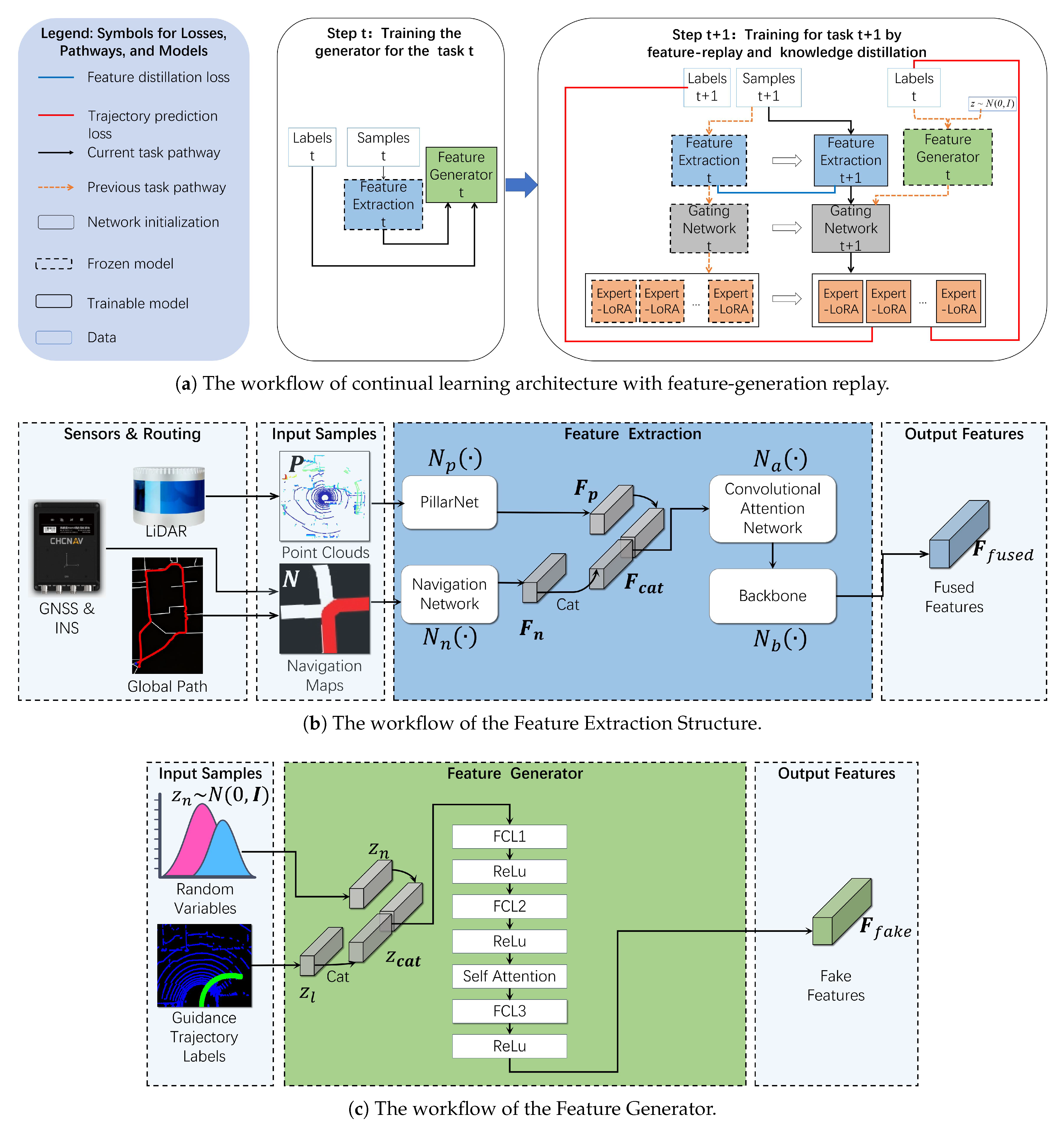
The core of the continual learning architecture based on feature generation and playback is the combination of feature playback, knowledge distillation of features, and transfer learning of weight initialization of the generative network. As shown in Figure 3a, the process of continual learning for a current task is divided into two key elements: (a) Feature replay of the generator: the generator of task t is trained to generate features for task t, which are used to train task $t+1$ instead of the original data of task t. By replaying the features of previous tasks, the model can review the knowledge of previous tasks while learning the current task so as to effectively alleviate catastrophic forgetting. Compared with the sample replay method, this method does not need to store training samples, which effectively reduces the storage cost. (b) Knowledge distillation of features: Knowledge distillation preserves the knowledge of the old task by restricting the consistency of the output features of the new and old models. As shown in the figure, we force the feature extractor $F_t$ of the current task model to stay close to the feature extractor $F_{t+1}$ of the old task through $L2$-loss (Euclidean distance), ensuring the feature representation stability of the feature extractor of the current task model for the previous task. The detailed calculation formula is presented in Equation (15).

Additionally, transfer learning will also be used for parameter initialization: When performing model training for task $t+1$, we take the corresponding model weights of the model for task t as the initial weights for the new model. The reason is that the model of task t has been fully trained, and its weights already contain rich general feature representations. Using these weights as the initial values of the target task, the model can accelerate convergence and improve the performance of the model.

3.2. Structure-Enhanced Feature Generation Method

We adopt a structure-enhanced feature generation method. On the one hand, the feature generator is built on a Multi-Layer Perceptron (MLP) integrated with a self-attention module [30] , as shown in Figure 3c. The feature generator has two inputs. The first is a random vector $z_n\in {\mathbb{R}}^{N_t}$ that follows a Gaussian distribution, and the second is a guidance trajectory label $g_l\in {\mathbb{R}}^{N_t}$. These two variables are concatenated to form a concatenated variable $z_{cat}\in {\mathbb{R}}^{2N_t}$. The output of the feature generator is a fake feature ${\mathbf{F}}_{fake}\in {\mathbb{R}}^{d_r}$, which is used to simulate the real feature ${\mathbf{F}}_{fused}\in {\mathbb{R}}^{d_r}$ generated by the feature extractor.

Conventional MLP models fail to characterize the correlation information across different dimensions and positions in features. To address this limitation, we incorporate a self-attention module to capture cross-dimensional and positional dependencies, enabling the generator to focus on the relationships between different elements in the feature vector.

The core of the self-attention module lies in the matrix operation of query ($\mathbf{Q}$), key ($\mathbf{K}$), and value ($\mathbf{V}$), which enables each position in the sequence to pay attention to the information of all other positions, and ultimately outputs the weighted features. The complete calculation process can be decomposed into the following four key steps.

Firstly, after inputting the feature ${\mathbf{F}}_{in}\in {\mathbb{R}}^{N_b\times d_h}$, three independent linear layers ${\mathbf{W}}_q\in {\mathbb{R}}^{d_h\times d_k},{\mathbf{W}}_k\in {\mathbb{R}}^{d_h\times d_k},{\mathbf{W}}_v\in {\mathbb{R}}^{d_h\times d_k}$ are applied, which, respectively, generate the query matrix $\mathbf{Q}$, the key matrix $\mathbf{K}$, and the value matrix $\mathbf{V}$:

$$\begin{array}{cc}\hfill \mathbf{Q}& ={\mathbf{F}}_{in}{\mathbf{W}}_q\hfill \\ \hfill \mathbf{K}& ={\mathbf{F}}_{in}{\mathbf{W}}_k\hfill \\ \hfill \mathbf{V}& ={\mathbf{F}}_{in}{\mathbf{W}}_v,\hfill \end{array}$$

(1)

where the size of $\mathbf{Q}$, $\mathbf{K}$ and $\mathbf{V}$ is all ${\mathbb{R}}^{N_b\times d_k}$. The purpose of this step is to map the input to a space that is more suitable for calculating attention correlation.

Secondly, the attention score $\mathrm{S}\left(\mathbf{Q},\mathbf{K}\right)$ is used to measure the similarity between $\mathbf{Q}$ and $\mathbf{K}$. The higher the score, the more attention is paid to the $\mathbf{V}$ at the corresponding position. The formula for calculating the attention score is

$$\mathrm{S}\left(\mathbf{Q},\mathbf{K}\right)={\displaystyle \frac{\mathbf{Q}{\mathbf{K}}^T}{\sqrt{d_k}}},$$

(2)

where multiplying the matrix of $\mathbf{Q}$ with the transpose matrix of $\mathbf{K}$ results in a similarity matrix (denoted as $\mathbf{M}$) with a size of ${\mathbb{R}}^{N_b\times N_b}$. The element at position $(i,j)$ in the $\mathbf{M}$ represents the dot product of “the $\mathbf{Q}$ at the i-th position” and “the $\mathbf{K}$ at the j-th position”.

As for why $\mathbf{M}$ needs to be divided by $\sqrt{d_k}$, it is because when $d_k$ is relatively large, the numerical value of the dot product result of $\mathbf{Q}$ and $\mathbf{K}$ will be extremely large, causing the input of the Softmax function to fall into the saturation zone, where the gradient is close to zero. And the derivative of the Softmax function for large values approaches zero, making it difficult for the model to update the parameters. Furthermore, when $\mathbf{Q}$ and $\mathbf{K}$ follow an independent and identically distributed (i.i.d.) standard normal distribution, the expected value of their dot product is 0 and the variance is $d_k$. To keep the variance of the dot product constant, it is necessary to scale the dot product result by $\sqrt{d_k}$ (i.e., divide it by $\sqrt{d_k}$). This ensures that as $d_k$ increases, the dot product does not grow linearly but remains at a constant level.

Thirdly, the attention scores $\mathrm{S}\left(\mathbf{Q},\mathbf{K}\right)$ are converted into probability weight ${\mathbf{Attn}}_w$ through the Softmax function, such that the sum of the weights for all positions is 1, ensuring that the weights are in a reasonable distribution ratio. The formula for the converted attention probability weight is

$${\mathbf{Attn}}_w=\mathrm{Softmax}\left({\displaystyle \frac{\mathbf{Q}{\mathbf{K}}^T}{\sqrt{d_k}}}\right),$$

(3)

where ${\mathbf{Attn}}_w$ represents the probability weight, with the size of ${\mathbb{R}}^{N_b\times N_b}$. The element at position $(i,j)$ in ${\mathbf{Attn}}_w$ represents the attention weight of the i-th position towards the j-th position. The higher the weight, the greater the influence that the i-th position has on the calculation of the output, indicating that the information of the j-th position of $\mathbf{V}$ needs to be more incorporated at that position.

Finally, a weighted sum of the $\mathbf{V}$ matrix is computed using probability weight ${\mathbf{Attn}}_w$, yielding the final output ${\mathbf{F}}_{out}\in {\mathbb{R}}^{N_b\times d_k}$ for each position. The output at each position incorporates the $\mathbf{V}$ information from all positions. The formula for the final output is given by

$${\mathbf{F}}_{out}={\mathbf{Attn}}_w\mathbf{V},$$

(4)

where ${\mathbf{F}}_{out}$ denotes the final output matrix of the self-attention module. The i-th row represents the feature of the i-th position after integrating information from all positions.

On the other hand, we construct the structural loss of features, as shown in (5) , in terms of sparsity patterns and statistical distribution. The adversarial loss of traditional a Generative Adversarial Network (GAN) only focuses on the overall distribution matching and ignores the fine-grained structure inside the features. The true features are structurally sparse, while the features trained according to the adversarial loss may be randomly sparse.

$${\mathcal{L}}_{\mathrm{struct}}={\lambda }_1·{\mathcal{L}}_{\mathrm{mask}}+{\lambda }_2·{\mathcal{L}}_{\mathrm{value}},$$

(5)

where ${\lambda }_1$ and ${\lambda }_2$ denote the weights of ${\mathcal{L}}_{\mathrm{mask}}$ and ${\mathcal{L}}_{\mathrm{value}}$, respectively.

Firstly, in terms of sparsity pattern, we model which positions of the feature vector should be nonzero and the spatial correlation of non-zero positions. Jaccard distance [31] is a measure of the dissimilarity of two sets, which is scale-invariant and insensitive to specific values. We treat the representation of the feature vector as a binary mask (1 for non-zero elements and 0 for zero elements) and compute the Jaccard distance between the generated features and the true features (ranging from 0 to 1), as shown in Equation (6). A Jaccard distance closer to 1 indicates that the sparsity patterns of the two features are more similar, while a Jaccard distance closer to 0 indicates the opposite.

$${\mathcal{L}}_{\mathrm{mask}}=1-\mathrm{Jaccard}({\mathbf{M}}_{\mathbf{g}},{\mathbf{M}}_{\mathbf{r}}),$$

(6)

where ${\mathbf{M}}_{\mathbf{g}}\in {\mathbb{R}}^{d_r},{\mathbf{M}}_{\mathbf{r}}\in {\mathbb{R}}^{d_r}$ represent the non-zero mask for the generated features and the true features.

Secondly, in terms of statistical distribution, the distribution between the nonzero values of the feature vectors is mainly constrained. As shown in (7), the mean of the pointwise differences between the nonzero values of the generated and true features is computed, and the KL divergence between the generated distribution and the true distribution is computed. The non-zero value distribution of the generated features is in line with the true distribution.

$${\mathcal{L}}_{\mathrm{value}}=\mathrm{MSE}({\mathbf{Z}}_{\mathbf{g}},{\mathbf{Z}}_{\mathbf{r}})+\alpha ·\mathrm{KL}({\mathbf{P}}_{\mathbf{g}} \Vert {\mathbf{P}}_{\mathbf{r}}),$$

(7)

where ${\mathbf{Z}}_{\mathbf{g}}\in {\mathbb{R}}^{d_r}$ and ${\mathbf{Z}}_{\mathbf{r}}\in {\mathbb{R}}^{d_r}$ represent the sets of non-zero values for the generated and real features, respectively, and ${\mathbf{P}}_{\mathbf{g}}\in {\mathbb{R}}^1$ and ${\mathbf{P}}_{\mathbf{r}}\in {\mathbb{R}}^1$ represent the probability distribution (estimated by Gaussian kernel density estimation) of non-zero values. KL represents Kullback–Leibler Divergence, which is used to measure the difference between distributions. $\alpha$ represents the coefficient of KL. The sparse pattern addresses the question of which values are nonzero, while statistical distributions address the question of what values should reside in the nonzero positions. Together, these two components form a structural loss, which drives the generated features to be more aligned with the true features.

3.3. Dynamic Knowledge Expansion Model Based on MoE-LoRA

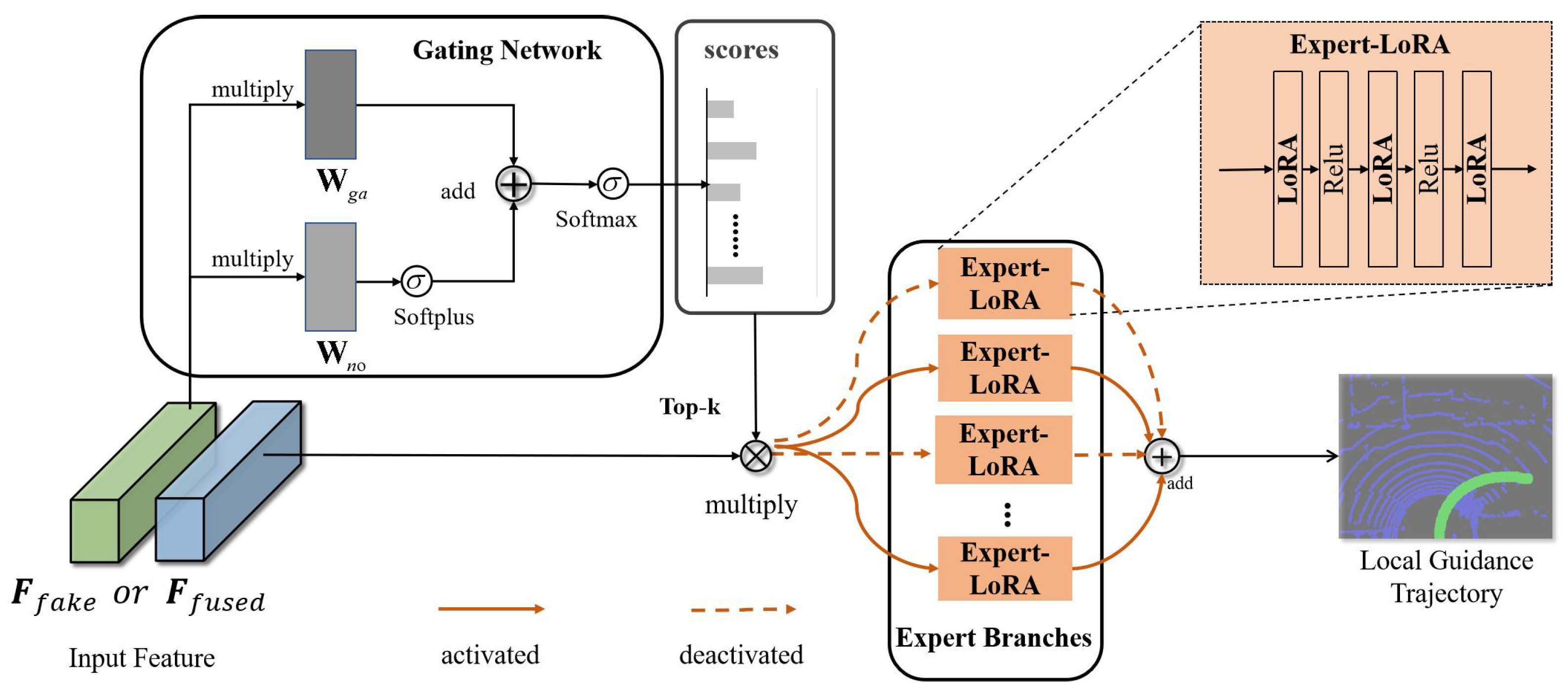
Dynamic Knowledge expansion Model based on MoE-LoRA: MoE [23] is a dynamic neural network architecture, which consists of a feature extractor, a gating structure, and an expert branch, as shown in Figure 4. The knowledge capacity of the network model can be improved by adding expert branches. At the same time, the gating structure can adaptively activate part of the expert branches so as to reduce the amount of calculation. LoRA [32] performs task-specific fine-tuning by multiplying two smaller matrices. When training a new task, we add the LoRA layer to the expert branch of MoE to form the MoE-LoRA structure so as to improve the knowledge capacity of the model and better improve the continual learning performance of the model.

Let $G_i(·)$ and $E_i(·)$ denote the output of the gating network and the output of the i-th expert branch respectively. Given the input feature ${\mathbf{F}}_{fused}\in {\mathbb{R}}^{d_r}$, the output $\mathbf{Y}\in {\mathbb{R}}^{N_t}$ of MoE can be expressed as follows:

$$\mathbf{Y}=\sum _{i=1}^{N_e}{G}_i\left({\mathbf{F}}_{fused}\right)E_i\left({\mathbf{F}}_{fused}\right),$$

(8)

where $N_e$ denotes the number of expert model branches. Whenever $G_i(·)=0$, $E_i(·)$ will not be computed. Leveraging the sparsity of $G_i(·)$, the computational cost is significantly reduced. The formulas for ${\mathbf{F}}_{fused}$, $G(·)$, and $E(·)$ are provided in Equations (9), (10) and (11), respectively.

3.3.1. Feature Extraction Structure

In our previous work [5], we validated the effectiveness of this feature extractor structure for the data-driven autonomous guidance problem. Therefore, this study will continue to adopt this structure. Below, we will briefly introduce the main components and workflow of the Feature Extraction Structure, while its specific design details and calculation formulas will not be reiterated.

Figure 3b illustrates the Feature Extraction Structure workflow of the guidance model. Point clouds $\mathbf{P}\in {\mathbb{R}}^{d_l\times N_l}$ and navigation maps $\mathbf{N}\in {\mathbb{R}}^{d_n\times H_n\times W_n}$ are obtained from LiDAR, GNSS&INS, and other sensors, serving as the input samples for the feature extractor. Here, $N_l$ represents the total number of points within a single point cloud frame. $d_l$ denotes the dimension of the LiDAR point cloud, which contains $\mathrm{location}(x,y,z)$ and reflectivity. $d_n$ represents the dimension of the navigation map. $W_n,H_n$ denote the width and the height of the navigation map, respectively. After feature extraction by PillarNet, Navigation Network, Convolutional Attention Network, and Backbone, the output feature ${\mathbf{F}}_{fused}\in {\mathbb{R}}^{d_r}$ is obtained.

Within the Feature Extraction Structure, a convolutional neural network is primarily utilized to extract features from both the LiDAR point cloud and the navigation map. Subsequently, the extracted features from these two sources are concatenated, and the channel and spatial attention modules are integrated to facilitate adaptive feature fusion. After applying a deep convolutional neural network to the fused features, high-dimensional features are generated.

Denoting the input LiDAR point cloud data as $\mathbf{P}\in {\mathbb{R}}^{d_l\times N_l}$, $N_l$ represents the total number of points within a single point cloud frame. $d_l$ denotes the dimension of the LiDAR point cloud, which contains $\mathrm{location}(x,y,z)$ and reflectivity. Let $\mathbf{N}\in {\mathbb{R}}^{d_n\times H_n\times W_n}$ represent the input navigation map. The output feature ${\mathbf{F}}_{fused}\in {\mathbb{R}}^{d_r}$ of the Feature Extraction Structure is calculated by

$$\begin{array}{cc}\hfill & {\mathbf{F}}_{fused}=N_b\left(N_a(N_p\left(\mathbf{P}\right),N_n\left(\mathbf{N}\right))\right),\hfill \end{array}$$

(9)

where $N_b(·),N_a(·),N_p(·),N_n(·)$ denotes the backbone network, convolutional attention network, pointpillar network, and navigation network, respectively.

3.3.2. Gating Network

The gating network is a neural network structure comprising a single data element as input and a weight as output. The weight indicates the extent to which the expert contributes to the processing of the input data. The top-k models are typically selected by modeling the probability distribution via softmax.

The gating network consists of two main components: sparsity, implemented by the activation module, and noise, implemented by the noise module. We use ${\mathbf{W}}_{ga}\in {\mathbb{R}}^{d_r\times N_e},{\mathbf{W}}_{no}\in {\mathbb{R}}^{d_r\times N_e}$ to denote the gating weights and noise weights of the gating network, respectively. $N_e$ denotes the number of expert model branches. $d_r$ denotes the dimension of the feature map from the backbone network in Equation (9). Then, the calculation of the gating network can be formulated by the following equations:

$$\left\{\begin{array}{cc}\hfill & {\mathcal{L}}_{noise}=Softplus({\mathbf{F}}_{fused}·{\mathbf{W}}_{no})\hfill \\ \hfill & N\left({\mathbf{F}}_{fused}\right)=({\mathbf{F}}_{fused}·{\mathbf{W}}_{ga})+{\mathcal{L}}_{noise}\hfill \\ \hfill & K(v_i,k)=\left\{\begin{array}{cc}{v}_i\hfill & \mathrm{if} v_i \mathrm{is} \mathrm{in} \mathrm{the} \mathrm{top} k \mathrm{elements} \mathrm{of} v\hfill \\ -\infty \hfill & \mathrm{otherwise}\hfill \end{array}\right.\hfill \\ \hfill & G\left({\mathbf{F}}_{fused}\right)=Softmax\left(K(N\left({\mathbf{F}}_{fused}\right),k)\right),\hfill \end{array}\right.$$

(10)

where $Softplus$ denotes the softplus activation function and $Softmax$ denotes the softmax activation function. ${\mathcal{L}}_{noise}$ denotes the noise regularization term. $N(·)$ denotes the noise module. $K(·,·)$ denotes the activation module.

3.3.3. Expert Branches with LoRA

The structure of the expert is a model based on a multilayer perceptron (MLP) with LoRA. Each MLP consists of three fully connected layers with LoRA and a Relu activation function. The output of the j-th fully connected layer of the i-th expert branch can be expressed in Equation (11). In practice, we add a LoRA structure to each fully connected layer of the expert branch.

$$\begin{array}{cc}\hfill & E_i^j\left(x\right)=W_i^{j}x+{\mathbf{B}}_i^j{\mathbf{A}}_i^{j}x\hfill \\ \hfill & E_i\left({\mathbf{F}}_{fused}\right)=E_i^{N_f}(\dots \left(E_i^3\left(E_i^2\left(E_i^1\left({\mathbf{F}}_{fused}\right)\right)\right)\right)),\hfill \end{array}$$

(11)

where $W_i^j$ represents of the original weights j-th fully connected layer of the i-th expert branch. $B_i,A_i$ represent the LoRA layer matrix of the i-th expert. $N_f$ represents the number of fully connected layers.

3.4. Loss Function

3.4.1. Loss Function of Feature-Generation Replay

During the training process of the guidance point prediction model, the loss function mainly includes trajectory prediction loss ${\mathcal{L}}_{pred}$ and feature distillation loss ${\mathcal{L}}_{feat}$.

First, we utilize the $L1$ loss function to quantify the trajectory discrepancy between the ground truth and the model’s predictions. For a batch of data comprising $N_b$ elements, the unreduced loss can be expressed as follows:

$${\mathcal{L}}_{tr}={\displaystyle \frac{1}{N_p}}\sum _{n=1}^{N_p}|y_i-g_i|,$$

(12)

where $N_p$ denotes the number of points of one trajectory. $g_i$ denotes ground truth, and $y_i$ denotes the prediction of the model.

The gating network tends to converge to a state where it repeatedly allocates substantial weights to the same limited set of experts. To address this issue, we introduce an importance score $S_{imp}$ for each expert—relative to a batch of training samples—which is calculated by summing the importance weights (output by the gating network) across the entire batch. We further define an importance loss ${\mathcal{L}}_{imp}$ as follows:

$$\left\{\begin{array}{cc}\hfill & S_{imp}=\sum _{x\in \mathbf{X}}G\left(x\right)\hfill \\ \hfill & {\mathcal{L}}_{imp}={\left(NormAndArr\left(S_{imp}\right)\right)}^2,\hfill \end{array}\right.$$

(13)

where $\mathbf{X}$ denotes the input features of the batch; $S_{imp}$ represents the expert importance score computed via batch-wise summation; and NormAndArr denotes the “normalization and arrangement” operation.

The importance loss ${\mathcal{L}}_{imp}$, weighted by the load-balancing scalar ${\alpha }_{imp}$, is incorporated into the model’s overall loss to balance the importance weights across all experts. Specifically, this prediction loss ${\mathcal{L}}_{pred}$ is the sum of the trajectory prediction loss ${\mathcal{L}}_{tr}$ and the weighted importance loss ${\alpha }_{imp}{\mathcal{L}}_{imp}$:

$$\begin{array}{c}\hfill {\mathcal{L}}_{pred}={\mathcal{L}}_{tr}+{\alpha }_{imp}{\mathcal{L}}_{imp}\end{array}$$

(14)

The feature distillation loss is calculated based on the ${\mathcal{L}}_2$ norm between the features of the current task and those of the previous task, which is expressed by the following equation:

$${\mathcal{L}}_{feat}\left({\mathcal{X}}_t\right)={\mathbb{E}}_{\mathbf{x}\sim {\mathcal{X}}_t}{∥F_t\left(\mathbf{x}\right)-F_{t-1}\left(\mathbf{x}\right)∥}_2,$$

(15)

where $F_t\left(\mathbf{x}\right)$ represents the features output by the feature extractor when the input data is $\mathbf{x}$ and the task is t.

The total loss is expressed by the following equation:

$$\begin{array}{c}\hfill {\mathcal{L}}_{all}={\mathcal{L}}_{pred}+{\mathcal{L}}_{feat}\end{array}$$

(16)

3.4.2. Loss Function of GAN

In the training of the GAN, there are two training stages: discriminator training and generator training.

First, when training the discriminator, the training objective is to output a high probability for the real feature $F_t\left(\mathbf{x}\right)$ and a low probability for the generated data $G_t\left(c,\mathbf{z}\right)$. Therefore, the loss function of the discriminator is designed as

$$\begin{array}{cc}\hfill {\mathcal{L}}_{D_1}\left({\mathcal{X}}_t\right)& =+{\mathbb{E}}_{z\sim p_z,c\in {\mathcal{C}}_t}\left[D_c\left(G_t(c,z)\right)\right]\hfill \\ \hfill & -{\mathbb{E}}_{x\sim D_t}\left[D_c\left(F\left(x\right)\right)\right],\hfill \end{array}$$

(17)

where ${\mathcal{X}}_t$ represents the input data set of task t. z denotes the input noise of the generator, following a standard normal distribution $p_z=\mathcal{N}(0,1)$. $c\in {\mathcal{C}}_t$ represents the specific class label in the label set ${\mathcal{C}}_t$ corresponding to task t. $G_t(c,z)$ denotes the “fake feature” generated by generator $G_t$ based on class c and noise z. $D_c(·)$ represents the discrimination branch of the discriminator for class c. $F\left(x\right)$ denotes the “real feature” sampled from the real data distribution $D_t$

Second, when training the generator, the training objective is twofold: on one hand, to make the generated feature $G_t(c,\mathbf{z})$ “fool” the discriminator as much as possible, i.e., to maximize $D_c\left(G_t(c,\mathbf{z})\right)$; on the other hand, to maintain structural rationality, which means minimizing the structural loss term ${\lambda }_{\mathrm{struct}}{\mathcal{L}}_{\mathrm{struct}}$. Therefore, the loss function of the discriminator is designed as

$$\begin{array}{cc}\hfill +{\mathcal{L}}_{G_t}\left({\mathcal{X}}_t\right)& =+{\lambda }_{\mathrm{struct}}{\mathcal{L}}_{\mathrm{struct}}\hfill \\ \hfill & -{\mathbb{E}}_{z\sim p_z,c\in {\mathcal{C}}_t}\left[D_c\left(G_t(c,z)\right)\right],\hfill \end{array}$$

(18)

where ${\lambda }_{\mathrm{struct}}$ represents the weight coefficient of the structural loss, used to balance the importance of “adversarial realism” and “structural rationality”. ${\mathcal{L}}_{\mathrm{struct}}$ denotes the structural loss, used to ensure that the structure of generated features conforms to prior knowledge. $G_t(c,z)$ denotes the “fake feature” generated by generator $G_t$ based on class c and noise z. $D_c(·)$ represents the discrimination branch of the discriminator for class c.

To present the details of our method more clearly, the symbols involved in the method, along with their descriptions and sizes, are presented in the Appendix A.

4. Experiments and Discussion

4.1. Model and Training Parameter Configuration

(1) Model Parameter. In the pillar network, the grid size is set to (0.5 m, 0.5 m, 4 m), and each grid is capped at 100 point clouds. The size of the convolution kernel here is specified as $1\times 1$. In the navigation network, the convolution kernel adopts a size of $3\times 3$. For the convolutional attention network, the convolution kernel maintains a size of $1\times 1$. In the backbone network, the convolution kernel has a size of $3\times 3$. The residual layers, which consist of four layers, each contain $(2,2,2,2)$ residual blocks. For the MoE structure, the Multi-Layer Perceptron (MLP) comprises 256 neurons for its input layer, 128 neurons for the hidden layer, and 40 neurons for the output layer. The additional parameters cited in Section 3 are elaborated in Table 1.

(2) Training Parameter. The batch size used for model training is related to the GPU of the computer employed for training. During model training in the simulation environment, an NVIDIA RTX 3090 GPU is used; with its 24 GB of video RAM (VRAM), the batch size can be increased, and it is set to 30 in the experiment. The VRAM usage at different stages of model training is as follows: during the initial training phase of the guidance model, it is 8271 Mb; during the GAN training phase, it is 18,555 Mb; and during the incremental learning training phase, it is 16,435 Mb. When the algorithm needs to be deployed on an Unmanned Ground Vehicle (UGV) in a real-world environment, different batch sizes must be selected based on the computing resources of the UGV’s on-board computer. For example, the on-board computer used in this study has 16 GB of VRAM, so a batch size of 20 is chosen for training. Under this configuration, the VRAM usage at different training stages is 6135 Mb during the initial training phase of the guidance model, 13,351 Mb during the GAN training phase, and 10,719 Mb during the incremental learning training phase.

Table 1. Variable definition and value assignment.

Symbol	Description	Value/Shape
$N_b$	Batch size	-
$N_t$	Number of trajectory points	40
$N_e$	Number of expert branches	4
$d_k$	Dimension of queries and keys in Self-Attention module	256
$d_h$	Dimension of hidden layer of MLP	256
$d_l$	Dimension of LiDAR point cloud	4
$d_r$	Dimension of feature map from backbone network	512
$d_n$	Dimension of the navigation map	3
$N_l$	Number of points in one point cloud frame	51,000
$H_n$	Height of the navigation map	100
$W_n$	Width of the navigation map	100
${\alpha }_{imp}$	Load-balancing scalar	0.01
${\lambda }_1$	Weight of ${\mathcal{L}}_{\mathrm{mask}}$	1.0
${\lambda }_2$	Weight of ${\mathcal{L}}_{\mathrm{value}}$	1.0
$\alpha$	Coefficient of KL	0.1

Table 1. Variable definition and value assignment.

Symbol	Description	Value/Shape
$N_b$	Batch size	-
$N_t$	Number of trajectory points	40
$N_e$	Number of expert branches	4
$d_k$	Dimension of queries and keys in Self-Attention module	256
$d_h$	Dimension of hidden layer of MLP	256
$d_l$	Dimension of LiDAR point cloud	4
$d_r$	Dimension of feature map from backbone network	512
$d_n$	Dimension of the navigation map	3
$N_l$	Number of points in one point cloud frame	51,000
$H_n$	Height of the navigation map	100
$W_n$	Width of the navigation map	100
${\alpha }_{imp}$	Load-balancing scalar	0.01
${\lambda }_1$	Weight of ${\mathcal{L}}_{\mathrm{mask}}$	1.0
${\lambda }_2$	Weight of ${\mathcal{L}}_{\mathrm{value}}$	1.0
$\alpha$	Coefficient of KL	0.1

If the on-board computing resources are still limited, the batch size can be further reduced, and the model can be updated using methods such as gradient accumulation updates. This approach sacrifices some training time in exchange for model performance, which is a necessary trade-off in engineering applications. When the batch size is set to 10, the VRAM usage is 5919 Mb during the initial training phase of the guidance model, 9639 Mb during the GAN training phase, and 6085 Mb during the incremental learning training phase. In addition, the learning rate needs to be correlated with the batch size. Generally, based on empirical experience, a smaller batch size requires a smaller learning rate; otherwise, it will cause oscillations in the training curve. When the batch size is doubled, the learning rate can be adjusted by a factor of 1.5∼2. When the batch size is set to 30, the learning rate is chosen as $0.001$. This decision is based on the fact that the Adam optimizer balances convergence speed and stability through “momentum” and “adaptive learning rate,” and $0.001$ is an empirically validated intermediate optimal value from extensive experiments.

In summary, the above content clarifies the core correlation between batch size, hardware VRAM resources, and learning rate during model training, while detailed parameters (including scenario-specific batch sizes, corresponding learning rates, and VRAM usage at each training stage) are tabulated in

Table 2. Key Training Parameters Under Different Scenarios.

Scenario	Batch Size	Learning Rate	VRAM (Mb)
			Initial Training	GAN Training	Incremental Training
Simulation	30	0.001	8271	18,555	16,435
Real UGV	20	0.0007	6135	13,351	10,719
Resource-Constrained UGV	10	0.0004	5919	9639	6085

for quick reference.

4.2. Evaluation Metrics

In the domain-incremental learning scenario of waypoint generation models, the core objectives include adapting to new domains, retaining knowledge of old domains, and enabling efficient deployment. To comprehensively assess the performance of such models, this study integrates existing evaluation metrics and supplements them to form a more complete evaluation system, as detailed below.

The sub-indicators are designed to target the four core objectives of domain-incremental learning: covering basic task performance, knowledge retention capability, and resource efficiency, as well as the adaptation effect to new domains.

• Average Trajectory Error (ATE).
• Average Forgetting Measure (AFM).
• Storage Utilization (SU).
• New Domain Performance Improvement (NPI).

4.2.1. Average Trajectory Error (ATE)

Average Trajectory Error (ATE) was introduced in our previous work [5]. ATE quantifies the accuracy of the guidance trajectory generated by the model across all currently available domains (including both new and old domains). It directly reflects the basic performance of the guidance trajectory generation task, serving as a fundamental indicator to measure whether the model meets the functional requirements of trajectory guidance.

$$\left\{\begin{array}{cc}\hfill & TE={\displaystyle \frac{1}{N_p}}\sum _{n=1}^{N_p}|y_n-g_n|,\hfill \\ \hfill & AT{E}_k={\displaystyle \frac{1}{N_k}}\sum _{i=1}^{N_k}T{E}_i,\hfill \end{array}\right.$$

(19)

where $N_p$ denotes the number of points of one trajectory (we set it to 40 in this paper). $g_n\in \mathbf{G}$ denotes ground truth, and $y_n\in \mathbf{Y}$ denotes the prediction of the model. $AT{E}_k$ denotes the ATE value for the k-th task. $T{E}_i$ denotes the trajectory error on the i-th frame in the k-th task. $N_k$ denotes the number of frames in the k-th task.

4.2.2. Average Forgetting Measure (AFM)

The Forgetting Measure (FM) calculates the degree of performance degradation of the model on old domains after learning new domains [33]. The Average Forgetting Measure (AFM) is the average value of all FM values. It specifically measures the model’s ability to retain knowledge acquired from old domains during the incremental learning process, which is a key indicator to evaluate the "catastrophic forgetting" problem in incremental learning.

The FM value of the j-th task at the point when training reaches the k-th task is $f_j^k$:

$$\left\{\begin{array}{cc}\hfill & f_j^k=AT{E}_{j,k}-\underset{l\in \{1,\cdots ,k-1\}}{min}AT{E}_{j,l},\hspace{1em}\forall j<k,\hfill \\ \hfill & AF{M}_k={\displaystyle \frac{1}{k-1}}\sum _{j=1}^{k-1}{f}_j^k,\hfill \end{array}\right.$$

(20)

where $AT{E}_{j,k}$ represents the ATE of the j-th task at the point when training reaches the k-th task. $AF{M}_k$ denotes the AFM value for the k-th task. Due to the constraints of the formula, when proceeding to the k-th task, only the FM of the first $k-1$ tasks can be calculated, and the FM of the k-th task cannot be calculated.

4.2.3. Storage Utilization (SU)

Storage Utilization (SU) is defined as the ratio of the storage space occupied by the model during incremental learning to the storage space of the baseline model [34]. This indicator reflects the resource efficiency of the incremental learning algorithm, which is of great significance for the efficient deployment of the model in resource-constrained scenarios (e.g., edge devices).

It is calculated as the ratio of the model to the base model.

$$SU={\displaystyle \frac{S}{S_{base}}},$$

(21)

where $S,S_{base}$ denote the storage of the method and the baseline model, respectively.

4.2.4. New Domain Performance Improvement (NPI)

New Domain Performance Improvement (NPI) is a new indicator we propose, defined as the ratio of the performance difference—on the new domain—between the model after incremental learning and the basic model (i.e., the model trained exclusively on new domain data). Specifically, it measures the improvement that the incremental learning algorithm brings to the model’s ability to adapt to new domains and directly reflects whether the model has achieved effective adaptation to the new domain.

The NPI value of the j-th task at the point is ${\mathrm{NPI}}_j$ is

$$\left\{\begin{array}{cc}\hfill & NP{I}_j=max\left\{min\left\{1-{\displaystyle \frac{p_{\mathrm{new}}^j-p_{\mathrm{base}}}{p_{\mathrm{base}}}},1\right\},0\right\},\hspace{1em}\forall 1<j<=k,\hfill \\ \hfill & ANPI={\displaystyle \frac{1}{k-1}}\sum _{j=2}^{k}NP{I}_j,\hfill \end{array}\right.$$

(22)

where $p_{\mathrm{new}}^j$ represents the final performance of the model after incremental learning in the new domain. $p_{\mathrm{base}}$ represents the performance of the base model after it has been fully trained in the new domain. The Average New Domain Performance Improvement (ANPI) denotes the average of all the NPIs for all $k-1$ tasks. Due to the constraints of the formula, when proceeding to the k-th task, only the FM of the last $k-1$ tasks can be calculated, and the NPI of the first task cannot be calculated.

4.3. Datasets from Simulations

We selected five environments with significant spatial feature differences from the CARLA simulator [35], as shown in Figure 5. Different towns have significant differences in road structure, surrounding environment, road slope, etc., making them suitable as experimental data for domain incremental learning. The geographical and spatial distribution differences of each map are as follows:

• Map-1: A small town map featuring a “T-junction” as its main feature, with a small river flowing through it, dividing the town into two halves and surrounded by coniferous forests.
• Map-2: The largest map, embedded in the mountains, featuring a special “8” shape of endless expressways and connected ramps for urban areas.
• Map-3: A city environment map featuring elevated highways as ring roads, numerous two-lane urban roads and complex intersections, with numerous commercial buildings.
• Map-4: A map including long highways, lane exits, and “Michigan left turn” and other special intersections, used for testing complex highway conditions and special turns.
• Map-5: A map of a simulated rural community featuring simple intersections, unmarked roads, and large areas of green landscapes such as cornfields and windmills.

We collected data on the curvature of various guiding points on each map for a total of 10,000 frames, including 6000 frames of training data, 2000 frames of validation data, and 2000 frames of test data. In order to further enhance the differences in data distribution among different maps, we selected five datasets with significant differences through the method of trajectory error cross-validation. The data in the datasets include 32-beam LiDAR data, global positioning data, local maps, and ground truth of guidance trajectory. The relevant data can be found in https://gitee.com/cslibowen/carla_data (accessed on 1 October 2025).

Figure 5. Experimental scenarios in the CARLA simulator.

Figure 5. Experimental scenarios in the CARLA simulator.

4.4. Comparing Continual Learning Methods

In this section, we evaluate the performance of the method proposed in this study against both classical and state-of-the-art continual learning strategies, with a specific focus on data-driven autonomous guidance tasks. To ensure a rigorous and fair comparison, all methods were implemented using the same base model architecture: a hybrid encoder–decoder network, where the encoder processes multi-sensor data to extract environmental features, and the decoder outputs continuous guidance point coordinates.

The methods for comparison and the adaptations made for the data-driven autonomous guidance task are as follows:

• Learning without Forgetting (LwF) [36]: This method achieves the goal of retaining the performance of the old task while learning new tasks by combining knowledge distillation (with soft target constraints) and hard-label training for new tasks. It effectively addresses the catastrophic forgetting problem in continuous learning.
• L2 Regularization [37]: A classical parameter regularization method that applies a penalty on the magnitude of model parameters during training. For data-driven autonomous guidance under Domain-IL, it alleviates catastrophic forgetting by restricting drastic updates to parameters—specifically, limiting changes to encoder and decoder weights that are critical for generating accurate guidance points in prior domains, thereby preserving performance on old domains while learning new ones.
• Elastic Weight Consolidation (EWC) [37]: A well-established regularization-based continual learning approach. It first estimates the importance of each model parameter for guidance point generation in previously learned domains (using the Fisher information matrix, which quantifies how parameter changes affect prediction error in prior domains). When training on a new domain, it applies a task-specific penalty to parameters with high importance, “consolidating” their values to avoid forgetting the ability to generate accurate guidance points for old domains.
• Feature-Generated Replay (FgR) [38]: A generative replay variant optimized for storage efficiency. Instead of storing raw multi-sensor data from prior domains, it trains a separate generator to synthesize environmental feature representations (matching the encoder output of prior domain data). During new domain training, these generated features are fed into the decoder (paired with their original guidance point labels) alongside new domain features, enabling the model to retain guidance point generation performance for old domains while reducing storage overhead compared to raw data replay.
• Example-based Replay (EbR) [16]: A representative experience replay method that stores a fixed-size subset of data samples from each prior domain—specifically, pairs of multi-sensor inputs and their corresponding ground-truth guidance points. When training on a new domain, the model is jointly trained on new domain data and the stored replay samples, directly mitigating forgetting by re-exposing the model to the sensor-guidance point relationships of old domains.

We trained the model on different datasets in sequence and conducted experiments using the aforementioned various incremental learning strategies. After each training session of the model, tests were conducted on all current test data. We will conduct a comprehensive and integrated assessment of all the methods based on the evaluation system designed in Section 4.2, including ATE, AFM, SU and NPI.

All models were implemented utilizing the PyTorch 1.8 framework. The Adam optimizer was employed to update the model weights, with a learning rate set to 0.001. Training of all models was conducted on NVIDIA RTX 3090 GPUs.

4.5. Domain-Incremental Learning Comparative Experiment on Simulator

We plotted the trajectory error data obtained from different continual learning strategies as a curve graph in Figure 6. Firstly, it can be observed that the overall trajectory error of the methods that incorporate replay (FgR, EbR, and ours) is lower than that of the regularization methods (L2, EWC, etc.). Specifically, the error of regularization-based methods (LwF, L2, EWC) increases rapidly as the number of maps increases. Among them, LwF’s error exceeds 0.40 in almost all maps; L2 and EWC are superior to LwF, but the errors in map-5 still reach 0.34 and 0.26, respectively. The reason for this phenomenon is that these methods only suppress forgetting through “parameter constraints” (such as L2 penalty, Fisher matrix protection), without an “old knowledge reuse” module. When training in a new domain, even if key parameters are constrained, they will gradually deviate from the knowledge of the old domain due to the lack of feedback from the old domain features and cannot utilize the rules of the old domain to assist learning in the new domain, resulting in a sharp increase in error when the data distribution of the new domain shifts. The error of the replaying-based methods (FgR, EbR, ours) increases slowly and steadily as the number of domains increases. Among them, ours always maintains the lowest error, with only 0.18 for map-5. The errors of EbR and FgR are approximately 0.22 and 0.23, respectively, significantly lower than those of the regularization methods. These methods achieve “reusing old knowledge”, simultaneously “reviewing” the knowledge of old domains during training in new domains. This not only avoids excessive parameter overwriting but also utilizes the general features of old domains to assist the adaptation of new domains, thereby suppressing error accumulation.

Our curve is consistently lower than that of FgR and EbR, and it fluctuates the least. The reason lies in the fact that ours has addressed the key flaws of the latter two: EbR requires storing the original LiDAR point cloud and map data but is limited by the sample storage capacity. It cannot cover all scenarios in the old domain, resulting in incomplete review and higher error rates than ours. FgR does not require storing the original data; its model is unchangeable and lacks scalability, leading to insufficient knowledge capacity and higher error than ours.

Table 3. Comparison experiments on the CARLA dataset for different continual learning strategies.

Method	ATE (∘)					Average (∘) ${\downarrow }^1$
	Map-1	Map-2	Map-3	Map-4	Map-5
LwF	0.1571	0.4804	0.4390	0.4290	0.4293	0.3870
L2	0.1745	0.3678	0.2868	0.3685	0.3361	0.3067
EWC	0.1871	0.2685	0.2545	0.2503	0.2620	0.2445
FgR	0.1354	0.2709	0.2428	0.2355	0.2258	0.2221
EbR	0.1524	0.2296	0.2104	0.2291	0.2219	0.2087
Ours	0.0941	0.2035	0.1703	0.1840	0.1842	0.1672

¹ The downward arrow indicates that the smaller the value, the better the performance (applicable to all tables).

provides a detailed list of the trajectory error values for different strategies on each map. We averaged the trajectory errors of each method across the five maps, and this resulted in ATE. The results show that our method has the lowest ATE, and as the number of tasks increases, the error increases slowly and with small fluctuations. It demonstrates better error control and stability in incremental learning, indicating that our method has significant advantages.

Next, we calculated the Forgetting Measure (FM) for various methods. According to the description in Section 4.2.2, we counted the FM for all methods on each map and calculated the Average Forgetting Measure (AFM) for all tasks using Equation (20). The results are listed in

Table 4. Forgetting measure on the CARLA dataset for different continual learning strategies.

Method	FM (∘)					AFM (∘) ↓
	Map-1	Map-2	Map-3	Map-4	Map-5 1
LwF	0.2844	0.0220	0.0081	0.0050	-	0.0799
L2	0.0334	0.0609	0.0648	0.0010	-	0.0400
EWC	0.0795	0.0443	0.1332	0.0620	-	0.0798
FgR	0.0876	0.0227	0.0460	0.0456	-	0.0505
EbR	0.0944	0.0000	0.0286	0.0407	-	0.0409
Ours	0.0342	0.0175	0.0488	0.0234	-	0.0310

¹ Since AFM can only calculate the first $k-1(k=5)$ maps, the FM on Map-5 cannot be calculated.

. The results show that although our method is not the lowest FM in each map, the average AFM across all tasks is the best. This demonstrates the long-term learning ability of our method. From Table 4, it can also be seen that LwF has a smaller FM value in map-3 and map-4 but a larger FM value in task 1. L2 has a smaller FM value in map-4 but a larger FM value in map-2 and map-3. Our method maintains a low FM value across the four maps, demonstrating that our method has a stronger ability to resist forgetting in continuous task continual learning. The core reason lies in the expert isolation design of MoE, where the parameters of the old domain experts are frozen and the new domain knowledge is stored in the newly added experts, thereby alleviating parameter-overwriting-type forgetting.

We then calculated the Storage Utilization (SU) for each method, and the results are shown in

Table 5. Storage usage for different continual learning strategies.

Method	Cache Sample (Mb)	Base Model (Mb)	All (Mb)	SU ↓
baseline	0	43.85	43.85	1.00
LwF	0	43.85	43.85	1.00
L2	0	43.85	43.85	1.00
EWC	1000	43.85	1043.85	23.81
FgR	0	105.16	105.16	2.40
EbR	750	43.85	793.85	18.10
Ours	0	107.08	107.08	2.44

.

First, we calculated the storage usage of the cache samples. The EWC method requires maintaining a Fisher matrix, which necessitates caching the samples from the previous task. EbR, however, requires the direct replay of old task samples when learning new tasks. For other methods that do not need to cache samples, the storage occupation of caching samples is zero. Our method does not require replaying samples either, so this item’s occupation is also zero.

Second, we calculated the storage usage of the model. Since LwF, L2, EWC and EbR all use the base model, the storage occupation of the model is the same as that of the base model. FgR and our method both require a generator to generate the model, so our base model has an additional part of storage occupation compared to the base model.

Finally, we add up the storage occupancy of the cache samples and the model to obtain the total storage occupancy. Then, using Equation (21), we calculate the Storage Utilization (SU) corresponding to each method. It is shown that although the SU value of our method is slightly higher than that of methods that only use the basic model (such as LwF and L2), our method outperforms the methods that require samples (such as EWC and EbR).

In order to assess the model’s adaptability to new domains, we calculated the New Domain Performance Improvement (NPI) value and the average NPI value (ANPI) based on Section 4.2.4.

Based on Equation (22), the NPI values corresponding to map-2 to map-5 were calculated, and then the ANPI was computed. The calculation results are presented in

Table 6. ANPI for different continual learning strategies.

Method	NPI					ANPI ↑ 2
	Map-1 1	Map-2	Map-3	Map-4	Map-5
LwF	-	0.0000	0.0000	0.5905	0.0000	0.1968
L2	-	0.5183	0.8801	0.5717	0.0000	0.6567
EWC	-	0.4104	1.0000	1.0000	1.0000	0.8035
FgR	-	0.2312	0.7316	1.0000	0.4352	0.6543
EbR	-	0.0000	0.9924	1.0000	1.0000	0.6641
Ours	-	0.6281	1.0000	1.0000	1.0000	0.8760

¹ Since NPI can only calculate the last $k-1(k=5)$ maps, therefore, the NPI on map-1 is unable to calculate. ² The upward arrow indicates that the larger the value, the better the performance (applicable to all tables).

. The results show that the NPI values of our method on map-3, map-4, and map-5 are all the highest value of 1, indicating that the performance of our method after training on the new domain is superior to the base model and demonstrating that our method has good adaptability to the new domain.

4.6. Ablation Experiment

4.6.1. Comparative Analysis on Generators of GAN

In order to investigate the influence of the training frequency of the generator in GAN on the feature maps, we conducted experiments with three parameters, n = 0.1, n = 0.5, and n = 1, and visualized the generated feature maps. As shown in Figure 7, the larger the parameter n of the training frequency, the closer the generated feature map is to the real feature. From the sparsity of the features in the figure, it can be seen that the more fully the generator is trained, the denser the generated feature is, and the less fully the generator is trained, the sparser the generated feature is.

To make the generated features closer to the real features, in Section 3.2, we proposed an improved method for the attention module and the structural loss. We conducted ablation experiments to verify the effectiveness of this method. To quantitatively evaluate the impact of different strategies on feature representation, we calculated the Euclidean distance between the generated features of $N=100$ frames and the corresponding real features as a quantitative standard to assess the performance of the generator.

Table 7. The ablation experiment results of the self-attention and structural loss.

Method	Euclidean Distance ↓
Original	4.137 (0.00%)
+Self-attention	4.326 (+4.57%)
+Structural loss	4.104 (−0.80%)
+Self-attention +Structural loss	4.070 (−1.62%)

shows that without additional strategies, the Euclidean distance is $4.137$; only introducing the self-attention module, the distance rises to $4.326$, and the deviation of the features from the real values increases; only adding the structural loss, the distance drops to $4.104$, and the features are closer to the real ones; when the self-attention module and the structural loss are combined, the distance further shrinks to $4.070$. It can be seen that the structural loss can effectively optimize the feature representation, while the self-attention module acting alone is likely to cause the features to deviate, and the synergy of the two can significantly improve the fit between the features and the real values, demonstrating the advantage of strategy integration.

4.6.2. Comparative Analysis on Experts of MoE

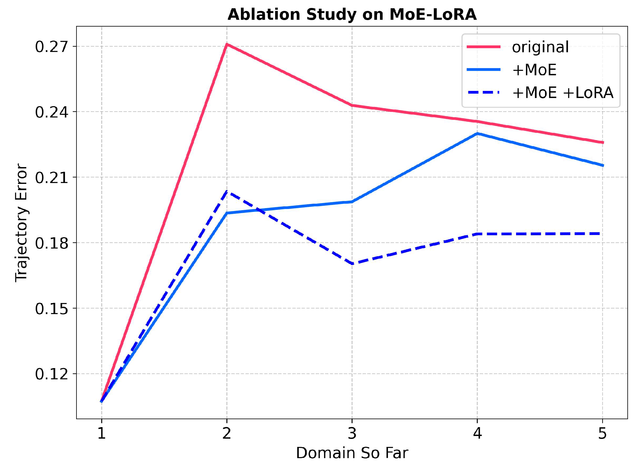
To verify the effectiveness of the combination of MoE and LoRA layers, we conducted the following ablation experiments. Figure 8 depicts trajectory error curves for incremental learning under different methods. The red solid line (original) shows higher initial error growth, while the blue solid line (+MoE) and blue dotted line (+MoE + LoRA) exhibit better performance, with the latter achieving lower and more stable errors.

Table 8. The ablation experiment results of the MoE module and the LoRA module.

Method	ATE id					Average (∘) ↓
	Map-1	Map-2	Map-3	Map-4	Map-5
Original	0.1354	0.2709	0.2428	0.2355	0.2258	0.22208 (0.00%)
+MoE	0.0926	0.1936	0.1987	0.2300	0.2154	0.18606 (−16.22%)
+MoE +LoRA	0.0941	0.2035	0.1703	0.1840	0.1842	0.16722 (−24.70%)

presents ablation results across five maps: the Original method has relatively high errors; +MoE reduces errors compared to Original; and +MoE + LoRA further lowers errors, confirming that combining MoE and LoRA enhances model performance in incremental learning.

We observed that when moving onto Task 2, the performance of the (+MoE + LoRA) method was slightly inferior to that of the (+MoE) method. The possible reasons we analyzed are as follows: When the LoRA (Low-Rank Adaptation) module was introduced, although theoretically it could adapt to new tasks without significantly changing too many model parameters, when the number of tasks was relatively small (such as task so far being 2), it might cause the model to suffer from overfitting on the current small number of tasks.

4.7. Cross-Domain Autonomous Guidance Experiment in Real-World

4.7.1. Experimental Platform

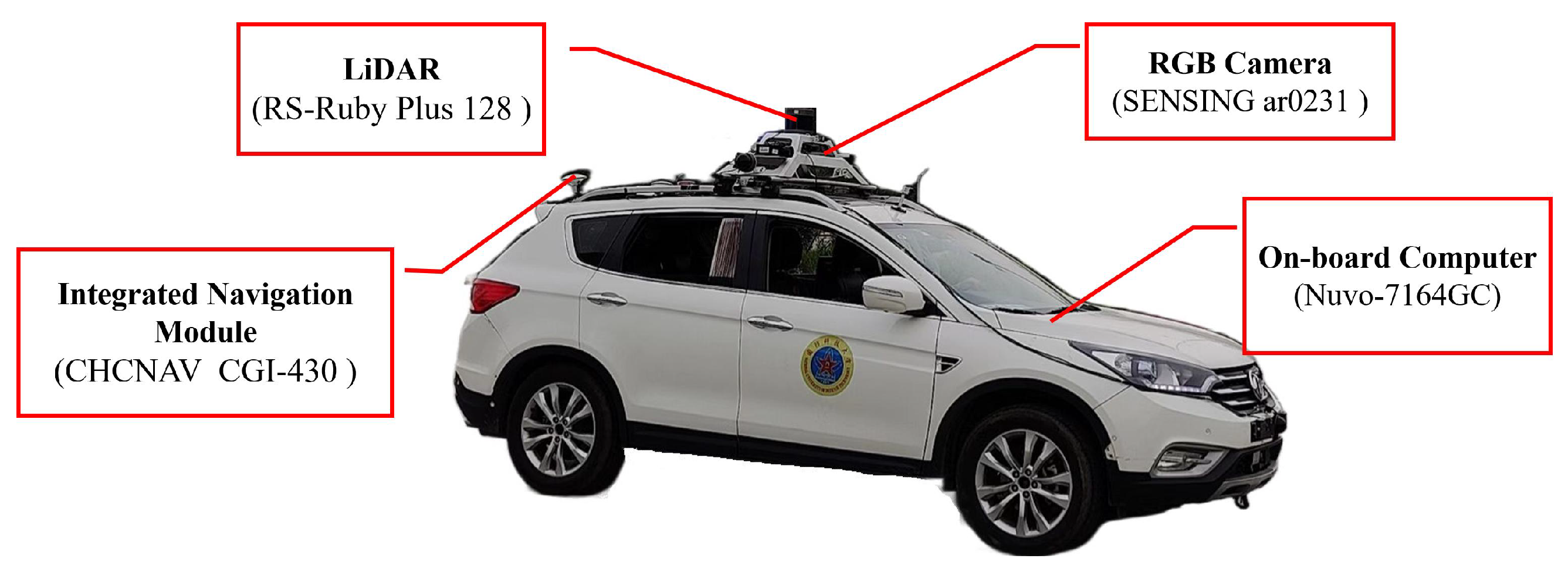
In real-world scenarios, the experimental platform employed in our work is illustrated in Figure 9. The experimental platform is equipped with a forward-facing RGB camera for monitoring the environment ahead of the vehicle, which outputs images at a resolution of $1920\times 1080$. It also features a LiDAR boasting 128 channels, a maximum detection range of 250 m, a 360° horizontal field of view (FOV), a 40° vertical FOV, and a ranging accuracy of $\pm 2$ cm. Additionally, a Wi-Fi module is integrated for communication purposes, along with a GNSS and INS integrated navigation system that provides global pose information for the vehicle. At the core of the UGV’s computing system lies a Nuvo-7164GC industrial control computer (ICC). This computer is fitted with a 9th-Gen Intel Core octa-core CPU and an NVIDIA Tesla T4 GPU—with the GPU featuring 16 GB of video memory and delivering $8.1$ TFLOPS of computing power under FP32 precision. The ICC is further configured with 64 GB of RAM and a 1 TB SSD for data storage and processing.

Additionally, since the traffic flow in the test environment is relatively dense, test vehicles will be equipped with safety officers for safety reasons. The safety officer sits in the driver’s seat and performs manual intervention promptly in case of danger.

4.7.2. Experimental Routes

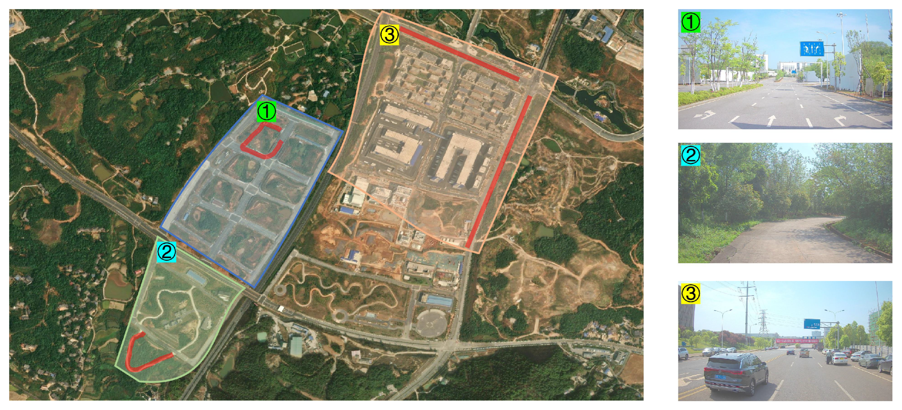
To further ascertain the efficacy of the methodology proposed in this paper on real UGVs, we conducted experimental validation in a real-world setting. As depicted in Figure 10, the realistic experimental environment comprises three scenarios.

The first scenario is closed roads in urban parks, featuring flat terrain and no traffic participants. The second scenario is rural roads, with undulating terrain, no lane markings, and no traffic participants. The third scenario is open urban roads, characterized by flat terrain and complex traffic participants (including pedestrians, motorcycles, and automobiles). One test route was selected for each of the first two test scenarios, while two vertical test routes were chosen for the third scenario. All these routes are marked in red in the figure.

In the offline experimental phase, data corresponding to the experimental route is first gathered. The initial 50% of this route’s data is allocated to model training and testing, with a 9:1 ratio maintained between the training set and the test set. Experiments are carried out sequentially in the order of Scenario 1, Scenario 2, and Scenario 3. After the model learns each new scenario, it is subjected to testing across all scenarios to validate the algorithm’s continuous learning capability. Once the offline experiment is completed, a qualitative analysis is conducted using trajectory errors as the evaluation basis.

In the real-time online experimental phase, the guidance model obtains real-time sensor data and sends the guidance trajectory to the planning and control module, which in turn guides the vehicle’s movement. Additionally, the test trajectory generated during the process is displayed on a satellite map to confirm its consistency with the globally planned trajectory.

4.7.3. Comparative Analysis on Real Environment

We conducted the same comparative experiment in a real environment. To avoid further elaboration, we directly list the ATE, AFM, SU, and ANPI values of each method in

Table 9. Performance on the real dataset for different continual learning strategies.

Method	ATE (∘) ↓	AFM (∘) ↓	SU ↓	ANPI ↑
LwF	0.1023	0.0334	1.00	0.50
L2	0.1149	0.0639	1.00	0.94
EWC	0.0551	0.0431	23.81	0.75
FgR	0.0298	0.0210	2.40	1.00
EbR	0.0212	0.0084	202.30	1.00
Ours	0.0163	0.0054	2.44	1.00

. The advantages of our method in the real world are mainly reflected in several aspects: it has excellent trajectory error control with an optimal ATE value of $0.0163$ (the smallest among all methods), enabling more accurate path planning compared to methods like L2 regularization ($0.1149$) and EWC ($0.0551$); it strongly suppresses the forgetting problem, as shown by its low AFM value of $0.0084$ across different scenarios—this value is only slightly higher than the optimal EbR ($0.0054$) and far lower than L2 ($0.0639$) and EWC ($0.0431$), ensuring the retention of previously learned knowledge; it features high storage efficiency, with an SU value of $2.44$, which is much lower than the excessive $202.30$ of EbR and comparable to the efficient FgR ($2.40$), reducing storage costs significantly while remaining competitive, and it has outstanding new domain adaptation capability, with an ANPI value of $1.00$ that matches the best-performing methods (FgR and EbR) and is higher than most others (e.g., LwF: $0.50$, L2: $0.94$, EWC: $0.75$), allowing it to quickly adapt to changes in complex real-world environments.

EbR achieves excellent performance in terms of AFM ($0.0054$, the optimal value) and ANPI ($1.00$), and its ATE ($0.0212$) is also among the top performers. However, it has an extremely high storage cost (SU value of $202.30$)—a figure that is two orders of magnitude higher than our method ($2.44$)—making it impractical for scenarios with limited storage resources. This indicates that EbR may have gained advantages in AFM and ATE at the expense of excessive storage usage. In contrast, ours strikes a balanced performance across ATE, AFM, SU, and ANPI: it maintains the smallest ATE ($0.0163$) for trajectory accuracy, a low AFM ($0.0084$) for knowledge retention, a moderate SU ($2.44$) for storage efficiency, and a full-score ANPI ($1.00$) for scenario adaptation. This multi-dimensional balance makes it more suitable for the complex constraints of the real world.

4.7.4. Visualization of Guidance Trajectory Result

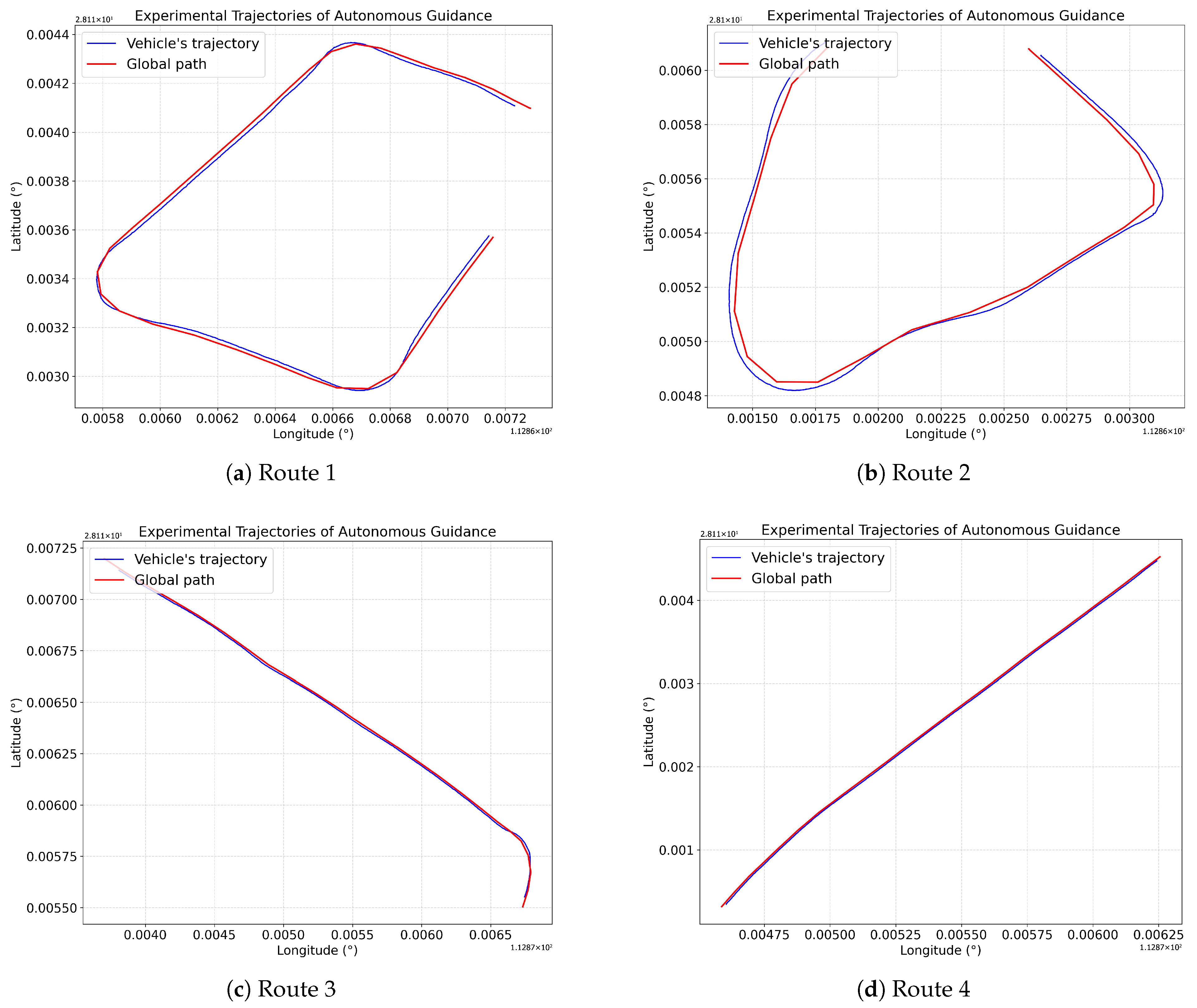
The trajectories of autonomously guided vehicles in the four test routes are compared with the global paths issued by the command and control system, intuitively demonstrating whether the vehicles travel along the expected path and avoiding the problem of “excellent numerical results but deviation in the actual path.” The experimental results of the four test routes are presented in Figure 11. It can be seen that the vehicles are able to complete autonomous guidance under the guidance of the global paths. Meanwhile, it is also noted that the curves do not completely overlap. This is because the global paths issued by the command and control system are rough trajectory points manually selected on the map, which have large errors and thus can only serve as reference trajectories rather than real executable ones. It can be observed that the trajectories generated by our guidance model are smoother and more in line with the requirements of vehicle dynamics.

To qualitatively analyze the effectiveness of the proposed guidance model, we visualize several representative data frames from each environment, as shown in Figure 12.

Route 1 features structured urban roads with clear lane markings and traffic signs, and the green local guidance trajectories accurately conform to the lane geometry, smoothly navigating straight segments and gentle curves. Route 2 is a narrower road surrounded by natural scenery with less explicit road structure, and our method successfully plans a trajectory that follows the winding road shape, demonstrating robustness in weakly structured environments. Route 3 features complex urban intersections with dynamic elements such as vehicles, traffic lights, and multi-directional traffic flows. The local guidance trajectories can dynamically adapt to traffic dynamics, smoothly merge into lanes, anticipate movements at intersections, and maintain safe distances from surrounding vehicles, demonstrating the model’s capability in highly complex scenarios. For Route 4, the road has obstacles and construction zones, with limited lane space. The local guidance trajectories lie completely within the restricted drivable area, avoid construction obstacles, and align with the remaining lane structure, which validates the model’s adaptability to constrained environments.

Across all routes, the local guidance trajectories consistently comply with the geometric constraints and dynamic conditions of specific scenarios, indicating that the incremental learning algorithm proposed in this paper can help the guidance model adapt to various environments, enabling the guidance model to effectively generate feasible and safe guidance paths in diverse environments.

4.8. Future Applications and Limitations

First, this study analyzes the application scenarios and advantages of the algorithm in practical Unmanned Ground Vehicles (UGVs). During actual autonomous guidance tasks for UGVs, the operating environment is not fixed. The task environment may change significantly due to the heterogeneity of geographical scenarios or the complexity of road topology. In such cases, the data domain expands with environmental changes, and traditional data-driven methods struggle to handle these scenarios. Merely learning the new data domain will cause the guidance model to suffer from “catastrophic forgetting” in terms of performance on the old data domain.

The method proposed in this study effectively addresses this issue. Experimental analysis shows that the method achieves the isolation of old and new model parameters through the Mixture-of-Experts–Low-Rank Adaptation (MoE-LoRA) structure, reducing the test error in both old and new environments by 24.7%. This method can be applied to the expansion of new autonomous guidance scenarios for UGVs, shortening the algorithm deployment time and improving the comprehensive guidance performance across old and new scenarios.

However, it is necessary to objectively recognize that the proposed method is not perfect and has certain limitations in practical application scenarios. For example, in UGV task scenarios, there is a large amount of high-dynamic or long-tailed distributed data—such as temporary road obstacles and sudden severe weather—which may cause the guidance model to output suboptimal or even dangerous paths. In such cases, the existing incremental learning algorithms alone cannot solve the problem. Therefore, in future research, an incremental learning method based on human–machine interaction can be designed, allowing UGVs to interact with human users. When emergencies occur, human feedback can be used to resolve problems and update the model.

5. Conclusions

This paper proposes a novel method that combines feature-generation replay with MoE to address catastrophic forgetting in data-driven autonomous guidance systems during continual learning. The proposed approach consists of three core components: First, a feature generation replay buffer architecture integrates feature replay, knowledge distillation, and weight initialization transfer learning. This design effectively reduces storage costs while maintaining the stability of the feature extractor—a critical advantage for the resource-constrained on-board computing platforms of UGVs. Second, an enhanced structural feature generation method adopts an MLP with a self-attention module and a custom structural loss function. It significantly improves the alignment between generated and real environmental features, such as LiDAR point cloud features and road topology features, ensuring the model retains accurate perception capabilities for the complex terrains and scenarios that UGVs frequently encounter. Third, a dynamic knowledge expansion model based on MoE-LoRA enhances the model’s knowledge capacity and continual learning performance by adding task-specific expert branches and incorporating LoRA fine-tuning. This allows the UGV guidance system to incrementally adapt to new operational scenarios, including urban structured roads, rural unmarked paths, and mountainous winding roads, without losing proficiency in previously learned environments.

Extensive domain-incremental learning experiments, conducted on both CARLA simulator environments, demonstrate that the proposed method outperforms representative continual learning approaches across multiple key metrics. These metrics include mean trajectory error, Average Forgetting Measure, Storage Utilization, and new domain performance improvement, which collectively validate the method’s effectiveness. The autonomous guidance experiments in real environments further verified the engineering application value of the method proposed in this paper. Across all test routes, the local guidance trajectories consistently comply with the geometric constraints and dynamic conditions of specific scenarios, indicating that the incremental learning algorithm proposed in this paper can help the guidance model adapt to various environments, enabling the guidance model to effectively generate feasible and safe guidance paths in diverse environments.

For UGV applications in particular, this method provides three critical enablers for practical deployment. First, its low storage overhead is compatible with the limited memory of UGVs’ on-board edge devices, avoiding the storage bottleneck of traditional sample-replay methods. Second, its strong anti-forgetting ability ensures UGVs can consistently perform well in multi-scenario missions—such as cross-regional patrols or disaster rescue without re-training from scratch. Third, its excellent new domain adaptability enables UGVs to quickly adjust to unexpected environmental changes, such as temporary road obstacles or uncharted rural terrain. Overall, this work lays a technical foundation for the long-term stable operation of data-driven UGVs’ autonomous guidance systems in complex, dynamic real-world scenarios. It also promotes the practical application of UGVs in fields like intelligent transportation, environmental monitoring, and emergency response.

References

1. Zhuang, H.; Fang, D.; Tong, K.; Liu, Y.; Zeng, Z.; Zhou, X.; Chen, C. Online Analytic Exemplar-Free Continual Learning with Large Models for Imbalanced Autonomous Driving Task. IEEE Trans. Veh. Technol. 2025, 74, 1949–1958. [Google Scholar] [CrossRef]
2. Bao, P.; Chen, Z.; Wang, J.; Dai, D.; Zhao, H. Lifelong Vehicle Trajectory Prediction Framework Based on Generative Replay. IEEE Trans. Intell. Transp. Syst. 2023, 24, 13729–13741. [Google Scholar] [CrossRef]
3. Liao, Y.; Xie, J.; Geiger, A. KITTI-360: A Novel Dataset and Benchmarks for Urban Scene Understanding in 2D and 3D. arXiv 2021, arXiv:2109.13410. [Google Scholar] [CrossRef]
4. Hanselmann, N.; Renz, K.; Chitta, K.; Bhattacharyya, A.; Geiger, A. KING: Generating Safety-Critical Driving Scenarios for Robust Imitation via Kinematics Gradients. In Computer Vision—ECCV 2022, Proceedings of the 17th European Conference, Tel Aviv, Israel, 23–27 October 2022; Springer: Cham, Switzerland, 2022; pp. 335–352. [Google Scholar]
5. Li, B.; Wu, T.; Yu, Y.; Li, J. End-to-End Autonomous Guidance Method Integrated with Mixture-of-Experts for Intelligent Vehicles. IEEE Trans. Veh. Technol. 2025, 1–15. [Google Scholar] [CrossRef]
6. Wang, L.; Zhang, X.; Su, H.; Zhu, J. A Comprehensive Survey of Continual Learning: Theory, Method and Application. IEEE Trans. Pattern Anal. Mach. Intell. 2024, 46, 5362–5383. [Google Scholar] [CrossRef]
7. Wickramasinghe, B.; Saha, G.; Roy, K. Continual Learning: A Review of Techniques, Challenges, and Future Directions. IEEE Trans. Artif. Intell. 2024, 5, 2526–2546. [Google Scholar] [CrossRef]
8. Nie, X.; Xu, S.; Liu, X.; Meng, G.; Huo, C.; Xiang, S. Bilateral Memory Consolidation for Continual Learning. In Proceedings of the 2023 IEEE/CVF Conference on Computer Vision and Pattern Recognition (CVPR), Vancouver, BC, Canada, 17–24 June 2023; pp. 16026–16035. [Google Scholar] [CrossRef]
9. Zhu, X.; Yi, J.; Zhang, L. Continual Learning With Unknown Task Boundary. IEEE Trans. Neural Netw. Learn. Syst. 2025, 36, 8140–8152. [Google Scholar] [CrossRef] [PubMed]
10. Pham, Q.; Liu, C.; Hoi, S.C.H. Continual Learning, Fast and Slow. IEEE Trans. Pattern Anal. Mach. Intell. 2024, 46, 134–149. [Google Scholar] [CrossRef]
11. Sorrenti, A.; Bellitto, G.; Salanitri, F.P.; Pennisi, M.; Palazzo, S.; Spampinato, C. Wake-Sleep Consolidated Learning. IEEE Trans. Neural Netw. Learn. Syst. 2025, 36, 12668–12679. [Google Scholar] [CrossRef]
12. Gao, Q.; Zhao, C.; Sun, Y.; Xi, T.; Zhang, G.; Ghanem, B.; Zhang, J. A Unified Continual Learning Framework with General Parameter-Efficient Tuning. In Proceedings of the 2023 IEEE/CVF International Conference on Computer Vision (ICCV), Paris, France, 1–6 October 2023; pp. 11449–11459. [Google Scholar] [CrossRef]
13. Krizhevsky, A. Learning Multiple Layers of Features from Tiny Images; University of Toronto: Toronto, ON, Canada, 2009. [Google Scholar]
14. Wang, L.; Xie, J.; Zhang, X.; Su, H.; Zhu, J. HiDe-PET: Continual Learning via Hierarchical Decomposition of Parameter-Efficient Tuning. IEEE Trans. Pattern Anal. Mach. Intell. 2025, 47, 6687–6702. [Google Scholar] [CrossRef] [PubMed]
15. Yu, D.; Zhang, M.; Li, M.; Zha, F.; Zhang, J.; Sun, L.; Huang, K. Contrastive Correlation Preserving Replay for Online Continual Learning. IEEE Trans. Circuits Syst. Video Technol. 2024, 34, 124–139. [Google Scholar] [CrossRef]
16. Chen, S.; Zhang, M.; Zhang, J.; Huang, K. Exemplar-Based Continual Learning via Contrastive Learning. IEEE Trans. Artif. Intell. 2024, 5, 3313–3324. [Google Scholar] [CrossRef]
17. Brignac, D.; Lobo, N.; Mahalanobis, A. Improving Replay Sample Selection and Storage for Less Forgetting in Continual Learning. In Proceedings of the 2023 IEEE/CVF International Conference on Computer Vision Workshops (ICCVW), Paris, France, 2–6 October 2023; pp. 3532–3541. [Google Scholar] [CrossRef]
18. Zhao, Y.; Saxena, D.; Cao, J. AdaptCL: Adaptive Continual Learning for Tackling Heterogeneity in Sequential Datasets. IEEE Trans. Neural Netw. Learn. Syst. 2025, 36, 2509–2522. [Google Scholar] [CrossRef]
19. Zhang, G.; Wang, L.; Kang, G.; Chen, L.; Wei, Y. SLCA: Slow Learner with Classifier Alignment for Continual Learning on a Pre-trained Model. In Proceedings of the 2023 IEEE/CVF International Conference on Computer Vision (ICCV), Paris, France, 1–6 October 2023; pp. 19091–19101. [Google Scholar] [CrossRef]
20. Yang, X.; Yu, H.; Gao, X.; Wang, H.; Zhang, J.; Li, T. Federated Continual Learning via Knowledge Fusion: A Survey. IEEE Trans. Knowl. Data Eng. 2024, 36, 3832–3850. [Google Scholar] [CrossRef]
21. Shahawy, M.; Benkhelifa, E.; White, D. Exploring the Intersection Between Neural Architecture Search and Continual Learning. IEEE Trans. Neural Netw. Learn. Syst. 2025, 36, 11776–11792. [Google Scholar] [CrossRef]
22. Son, J.; Lee, S.; Kim, G. When Meta-Learning Meets Online and Continual Learning: A Survey. IEEE Trans. Pattern Anal. Mach. Intell. 2025, 47, 413–432. [Google Scholar] [CrossRef]
23. Shazeer, N.; Mirhoseini, A.; Maziarz, K.; Davis, A.; Le, Q.; Hinton, G.; Dean, J. Outrageously Large Neural Networks: The Sparsely-Gated Mixture-of-Experts Layer. arXiv 2017, arXiv:1701.06538. [Google Scholar]
24. Liang, H.; Fan, Z.; Sarkar, R.; Jiang, Z.; Chen, T.; Zou, K.; Cheng, Y.; Hao, C.; Wang, Z. M3ViT: Mixture-of-Experts vision transformer for efficient multi-task learning with model-accelerator co-design. Adv. Neural Inf. Process. Syst. 2022, 35, 28441–28457. [Google Scholar]
25. Chen, Z.; Shen, Y.; Ding, M.; Chen, Z.; Zhao, H.; Learned-Miller, E.; Gan, C. Mod-Squad: Designing Mixtures of Experts As Modular Multi-Task Learners. In Proceedings of the 2023 IEEE Conference on Computer Vision and Pattern Recognition (CVPR), Vancouver, BC, Canada, 17–24 June 2023; pp. 11828–11837. [Google Scholar] [CrossRef]
26. Lu, X.; Liu, Q.; Xu, Y.; Zhou, A.; Huang, S.; Zhang, B.; Yan, J.; Li, H. Not All Experts are Equal: Efficient Expert Pruning and Skipping for Mixture-of-Experts Large Language Models. arXiv 2024, arXiv:2402.14800. [Google Scholar]
27. Zhang, Z.; Liu, X.; Cheng, H.; Xu, C.; Gao, J. Diversifying the Expert Knowledge for Task-Agnostic Pruning in Sparse Mixture-of-Experts. arXiv 2024, arXiv:2407.09590. [Google Scholar] [CrossRef]
28. Wang, J.; Lu, H.; Wang, A.; Yang, X.; Chen, Y.; He, D.; Wu, K. PhysMLE: Generalizable and Priors-Inclusive Multi-Task Remote Physiological Measurement. IEEE Trans. Pattern Anal. Mach. Intell. 2025, 47, 4908–4925. [Google Scholar] [CrossRef]
29. Luo, T.; Lei, J.; Lei, F.; Liu, W.; He, S.; Zhao, J.; Liu, K. MoELoRA: Contrastive Learning Guided Mixture of Experts on Parameter-Efficient Fine-Tuning for Large Language Models. arXiv 2024, arXiv:2402.12851. [Google Scholar]
30. Vaswani, A.; Shazeer, N.; Parmar, N.; Uszkoreit, J.; Jones, L.; Gomez, A.N.; Kaiser, L.; Polosukhin, I. Attention is all you need. In Proceedings of the 31st International Conference on Neural Information Processing Systems, NIPS’17, Long Beach, CA, USA, 4–9 December 2017; pp. 6000–6010. [Google Scholar]
31. Chen, Y.; Fan, Z.; Chen, Z.; Zhu, Y. CA-Jaccard: Camera-aware Jaccard Distance for Person Re-identification. In Proceedings of the 2024 IEEE/CVF Conference on Computer Vision and Pattern Recognition (CVPR), Seattle, WA, USA, 16–22 June 2024; pp. 17532–17541. [Google Scholar] [CrossRef]
32. Hu, E.; Shen, Y.; Wallis, P.; Allen-Zhu, Z.; Li, Y.; Wang, S.; Wang, L.; Chen, W. LoRA: Low-Rank Adaptation of Large Language Models. In Proceedings of the 2022 International Conference on Learning Representations (ICLR), Virtual, 25–29 April 2022; pp. 1–13. [Google Scholar]
33. Chaudhry, A.; Dokania, P.K.; Ajanthan, T.; Torr, P.H.S. Riemannian walk for incremental learning: Understanding forgetting and intransigence. In Proceedings of the 15th European Conference on Computer Vision (ECCV), Munich, Germany, 8–14 September 2018; pp. 556–572. [Google Scholar]
34. Liu, X.; Wu, C.; Menta, M.; Herranz, L.; Raducanu, B.; Bagdanov, A.D.; Jui, S.; van de Weijer, J. Generative Feature Replay For Class-Incremental Learning. In Proceedings of the IEEE/CVF Conference on Computer Vision and Pattern Recognition Workshops, New Orleans, LA, USA, 19–20 June2020; pp. 915–924. [Google Scholar]
35. Dosovitskiy, A.; Ros, G.; Codevilla, F.; Lopez, A.; Koltun, V. CARLA: An Open Urban Driving Simulator. In Proceedings of the 1st Annual Conference on Robot Learning, CoRL 2017, Mountain View, CA, USA, 13–15 November 2017; pp. 1–16. [Google Scholar]
36. Li, Z.; Hoiem, D. Learning without Forgetting. IEEE Trans. Pattern Anal. Mach. Intell. 2018, 40, 2935–2947. [Google Scholar] [CrossRef] [PubMed]
37. Kirkpatrick, J.; Pascanu, R.; Rabinowitz, N.; Veness, J.; Desjardins, G.; Rusu, A.A.; Milan, K.; Quan, J.; Ramalho, T.; Grabska-Barwinska, A.; et al. Overcoming catastrophic forgetting in neural networks. Proc. Natl. Acad. Sci. USA 2017, 114, 3521–3526. [Google Scholar] [CrossRef] [PubMed]
38. Zhang, Y.; Shao, M.; Shi, W.; Xia, H.; Xia, S. Autonomous Generative Feature Replay for Non-Exemplar Class-Incremental Learning. In Proceedings of the ICASSP 2024—2024 IEEE International Conference on Acoustics, Speech and Signal Processing (ICASSP), Seoul, Republic of Korea, 14–19 April 2024; pp. 5760–5764. [Google Scholar] [CrossRef]
Figure 1. The learning process of domain-incremental learning (DIL) for autonomous guidance in UGVs.
Drones 09 00757 g001
Figure 2. The data-driven autonomous guidance process.
Drones 09 00757 g002
Figure 3. The workflow of our proposed method.
Drones 09 00757 g003
Figure 4. The diagram of MoE-LoRA, showing the overall process from input features to output local guidance trajectory.
Drones 09 00757 g004
Figure 6. Test trajectory error curves of different continual learning algorithms. The blue dotted line represents the method proposed in this paper.
Drones 09 00757 g006
Figure 7. Visualization of feature maps under different training frequencies n: (a) Fake feature map when n = 0.1 . (b) Fake feature map when n = 0.5 . (c) Fake feature map when n = 1 . (d) Real feature map.
Drones 09 00757 g007
Figure 8. Comparison of trajectory error curves between the ordinary feature replay and the tests with added MoE and LoRA structures. The red solid line represents the feature replay method without adding MoE and LoRA. The blue solid line represents the feature replay method for increasing MoE. The blue dotted line represents the feature replay method that increases MoE and LoRA.
Drones 09 00757 g008
Figure 9. Experimental platform.
Drones 09 00757 g009
Figure 10. Three real experimental scenarios: Scenario 3 with two perpendicular test routes; Scenarios 1 and 2 each with one test route.
Drones 09 00757 g010
Figure 11. Results of the global projection of guidance trajectories.
Drones 09 00757 g011
Figure 12. Visualization of local guidance trajectories. The red lines represent the global path, while the green lines denote the local guidance trajectory generated by the guidance model.
Drones 09 00757 g012