Distributed Relative Pose Estimation for Multi-UAV Systems Based on Inertial Navigation and Data Link Fusion

Abstract

Accurate self-localization and mutual state estimation are essential for autonomous aerial swarm operations in cooperative exploration, target tracking, and search-and-rescue missions. However, achieving reliable formation positioning in GNSS-denied environments remains a significant challenge. This paper proposes a UAV formation positioning system that integrates inertial navigation with data link-based relative measurements to improve positioning accuracy. Each UAV independently estimates its flight state in real time using onboard IMU data through an inertial navigation fusion method. The estimated states are then transmitted to other UAVs in the formation via a data link, which also provides relative position measurements. Upon receiving data link information, each UAV filters erroneous measurements, time aligns them with its state estimates, and constructs a relative pose optimization factor graph for real-time state estimation. Furthermore, a data selection strategy and a sliding window algorithm are implemented to control data accumulation and mitigate inertial navigation drift. The proposed method is validated through both simulations and real-world two-UAV formation flight experiments. The experimental results demonstrate that the system achieves a $76\%$ reduction in positioning error compared to using data link measurements alone. This approach provides a robust and reliable solution for maintaining precise relative positioning in formation flight without reliance on GNSS.

1. Introduction

As the scope and complexity of unmanned aerial vehicle (UAV) missions continue to expand, single UAV operations face challenges in fulfilling the requirements of intricate tasks. Consequently, the cooperative operation of UAV formations has become a primary focus in current UAV research endeavors [1,2]. The precise relative positioning between UAVs within formations is crucial for ensuring the safety and reliability of missions, serving as a fundamental guarantee for tasks such as allocation, trajectory planning, and facilitating cooperative flight operations [3,4,5].

Currently, UAV formation flight typically relies on an integrated navigation approach combining Inertial Navigation Systems (INS) and Global Navigation Satellite Systems (GNSS) to determine absolute positions [6]. The relative positioning within the formation is derived from the absolute position information provided by INS [7,8]. However, in GNSS-denied environments, where signals are obstructed or disrupted, the formation must depend solely on INS for navigation [9]. While INS provide local positioning information, each UAV determines its position and attitude within its own independent navigation frame. This lack of a common reference frame makes it challenging to accurately estimate the relative positions between UAVs in the formation. Moreover, the cumulative drift in INS-based position and attitude estimates exacerbates this challenge, leading to significant degradation in positioning accuracy during long-duration missions [10]. Addressing these limitations, achieving high-precision autonomous relative positioning for formation flight in GNSS-denied scenarios has become a critical focus and technical challenge in aerospace navigation research [11].

In GNSS-denied environments, relative positioning methods for UAVs within a formation can be categorized into two groups based on the presence of inter-UAV communication: those that involve the exchange of flight state information and those that do not. For positioning methods that do not rely on inter-UAV communication, a common approach involves mutual recognition through the use of geometric markers, such as circles or rectangles, affixed to the UAV. Optical cameras detect these markers, and relative pose recognition algorithms analyze their pixel positions in captured images, comparing them with their known physical shapes to accurately compute the relative pose of each identified UAV [12,13]. To mitigate the effects of illumination variations during visual recognition and extend detection range, UAVs are often equipped with ultraviolet and infrared emitters, as well as Light Emitting Diode (LED) light strips, serving as markers. These markers are captured by cameras with corresponding filters, and subsequent image processing techniques are applied to detect, match, and accurately compute the relative positioning between UAVs [14,15,16]. Moreover, advancements in machine learning have facilitated the deployment of target recognition algorithms, such as YOLO (You Only Look Once), for relative positioning in UAV formations. This approach involves identifying the pixel coordinates of UAVs or markers within captured images and subsequently employing either the Perspective-n-Point algorithm for monocular cameras or visual vector computation methods for stereo cameras to determine relative positions [17,18,19]. While these methods are widely used in small-scale UAV clusters, their application to large-scale and complex flight missions is constrained by the limited detection range of onboard sensors. UAVs within a formation communicate with one another to exchange flight status and collect external environmental data. By matching image information, laser point cloud data, or landmark features acquired by different drones, the coordinate systems of multiple drones can be aligned, enabling accurate relative positioning among UAVs [20,21,22]. This method relies on the exchange of external environmental information between UAVs. However, the substantial volume of interactive data imposes constraints on communication bandwidth within the formation, making it challenging to scale the system to larger clusters or adapt to more complex operational environments.

Ranging data are one of the most commonly utilized sources for calculating the relative positions of UAVs. UAVs are typically equipped with short-range communication systems, which allow for the estimation of inter-UAV distances by measuring the time of flight (ToF) of transmitted signals. Common ranging technologies include ultra-wideband (UWB) and data link systems. UWB provides high-precision short-range ranging, while data link-based ranging is capable of covering distances of up to tens of kilometers, making it well-suited for long-range UAV formations [23,24,25]. In such formations, relative attitude estimation often relies on static data link anchors or a designated beacon UAV to infer the relative positions of all UAVs. However, these methods are constrained by anchor placement and beacon availability, limiting adaptability [26,27,28]. To overcome these limitations, UAV formations commonly integrate inertial navigation data with data link ranging for relative positioning, which can be categorized into three main approaches. The first approach involves the correction of inertial navigation using data link measurements, where data link distances refine inertial navigation parameters (position, velocity, and attitude) through filtering methods to enhance accuracy [29,30]. The second approach focuses on enhancing data link accuracy through inertial navigation, where inertial navigation data from multiple UAVs are combined to improve the precision of data link measurements, thereby enabling more accurate relative positioning [31]. The third approach is the tightly coupled integration of data link and inertial navigation, where short-term inertial data and data link measurements are fused using a filtering model to compute relative positions between UAVs [32,33].

However, the aforementioned methods present several significant limitations. First, they typically require mutual measurements between multiple UAVs or depend on external anchor points, imposing considerable constraints on system deployment. Second, optimization based on the integration of global poses from inertial navigation systems is prone to drift over time, particularly in extended-duration scenarios, which compromises overall accuracy. Furthermore, filtering methods used to estimate relative positions within a formation typically rely on only two states, making it challenging to mitigate measurement biases. Additionally, these methods have primarily been validated through short-duration, low-speed flight experiments in small-scale environments, resulting in low reliability. Lastly, these methods overlook issues such as sensor measurement time misalignment and outliers, rendering them challenging to directly apply in real-world mission scenarios.

Considering the limitations of existing methodologies, this paper proposes a relative attitude estimation method for UAV formations that integrates data link measurements with inertial navigation information. Each UAV estimates its flight state using an inertial navigation method and transmits this information to teammates via the data link, overcoming the deployment challenges associated with traditional methods. The proposed method constructs a relative position optimization factor graph model by utilizing short-term UAV flight states derived from inertial navigation integration and data link measurements within a sliding window. This approach reduces the impact of inertial navigation drift on relative pose estimation between UAVs, improving the algorithm’s accuracy and adaptability for long-duration operations. The factor graph model incorporates multiple adjacent states and measurements, reducing the influence of individual measurement errors. Furthermore, this method leverages the unique characteristics of trajectory intersections to eliminate bias in data link measurements, thereby enhancing both accuracy and robustness. To address the challenges of synchronizing state information from different sensor sources and handling measurement anomalies, the method employs spherical linear interpolation and motion modeling techniques. Flight experiments validate the effectiveness of the proposed approach, demonstrating a reduction in estimation error by more than $76\%$ compared to using data link measurements alone. Additionally, in contrast to traditional filtering methods, this approach effectively eliminates bias errors in data link measurements, further improving estimation accuracy.

2. Methodology

2.1. Problem Statement and Method Overview

UAV formations can estimate the relative position between UAVs by exchanging the GNSS global position data of UAVs or local positioning data provided by INS or vision systems. However, in complex flight environments, GNSS positioning data are susceptible to interference, leading to significant positioning inaccuracies. While INS can maintain normal operations in these environments, they are prone to drift over time, making them less suitable for extended-range missions. Vision-based relative positioning techniques are constrained by their detection range and may encounter difficulties in large-scale flight operations. To address the challenge of relative positioning between UAVs in formation during long-duration missions in GNSS-denied environments, this paper proposes a novel relative pose estimation method that integrates inertial navigation and datalink measurements. The overall framework of the proposed approach is illustrated in Figure 1. Each UAV in the formation is equipped with an formation positioning system consisting of four key modules: the inertial navigation module, the data link measurement process module, the time alignment module, and the relative positioning module.

Each UAV is equipped with an IMU sensor to capture acceleration and angular velocity data during flight. An inertial navigation integration algorithm is used to estimate its position and attitude in real time, and the estimated flight state is then transmitted to the data link module for further processing.

The integrated data link system equipped on each UAV within the formation facilitates bidirectional data link communication, enabling it to transmit its own flight status to teammates while receiving theirs. During communication, the data link can measure the relative distance, azimuth angle, and altitude angle of neighboring UAVs. To enhance accuracy, the data link measurement processing module filters out erroneous measurements and computes the relative positions of teammates based on the refined data.

The timestamps of sensor measurements from the IMU and data link are inherently asynchronous due to differences in system clocks across UAVs and variations in measurement frequencies between the IMU and data link. To address this issue, a decentralized time calibration method based on the peer delay mechanism in the Precision Time Protocol (PTP) is first employed to estimate the time offset. The data preprocessing module then aligns the timestamps by using the data link measurement time as a reference. Spherical linear interpolation is applied to synchronize the states of the two communicating UAVs to the reference timestamp. Additionally, the geometric characteristics of UAV states within the continuous time series are analyzed, and flight states with significant geometric variations are selected for optimization.

The relative positioning module processes data received from the data preprocessing module. Using the flight states of the UAV as vertices, it integrates the relative pose measurements obtained from the data link with the UAV state estimates to construct relative position error edges between UAVs. A relative pose factor graph, composed of these vertices and edges, is then established within a sliding window. The graph optimization method is employed to iteratively refine the relative pose estimates in real time, enhancing the accuracy of UAV positioning within the formation.

2.2. Symbol Description

The proposed UAV formation positioning algorithm involves multiple coordinate systems, each denoted as follows: the body frame coordinate system $\mathcal{B}$ (right-front-up), the Earth-centered Earth-fixed (ECEF) coordinate system $\mathcal{E}$, the navigation coordinate system $\mathcal{N}$ (East-North-Up, ENU), the data link coordinate system $\mathcal{D}$, and the inertial coordinate system $\mathcal{I}$. The body frame coordinate system is aligned with the IMU coordinate system. The transformation matrices between these coordinate systems are represented as $\mathit{T}\in SE(3)$.

$$\begin{array}{ccc}\hfill \mathit{T}& =\left[\begin{array}{cc}\mathit{R}& \mathit{t}\\ 0& 1\end{array}\right],\hfill & \hfill \left\{\mathit{R}\in SO(3),\mathit{t}\in \mathbb{R}\right\}.\end{array}$$

(1)

In this article, the symbols $\mathit{R}$ and $\mathit{t}$ represent the rotation matrix and translation vector, respectively. ${\mathit{T}}_{a,b}^k\in SE(3)$ represents the transformation matrix from coordinate system b at time k to coordinate system a. ${}_{ }{}^a\mathit{M}_{k,k-1}^{ }\in SE(3)$ signifies the motion transformation matrix of coordinate system a from time $k-1$ to k. Additionally, ${}_{ }{}^{a_{\mathcal{N}}}\mathit{p}_b^k\in {\mathbb{R}}^3$ represents the position of object b in the navigation coordinate system of object a at time k.

2.3. Data Link Ranging Model

Each UAV in the formation is equipped with a data link communication module, which enables the bidirectional exchange of flight state parameters between UAVs through electromagnetic wave propagation. The data link employs a bidirectional ranging technique to calculate the distance between the transmitting and receiving devices. This method leverages the propagation speed of electromagnetic waves in air—approximately $c=3\times {10}^8\mathrm{m}/\mathrm{s}$—to determine the separation distance by measuring the round-trip time of the signal. Simultaneously, the receiving end records its elevation angle and azimuth angle relative to the station center coordinate system of the transmitting device.

The entire data link communication cycle is completed in less than ${10}^{-4}$ s, rendering motion-induced measurement errors negligible due to the short duration compared to typical UAV movement dynamics. Consequently, the measured distance is considered accurate at the moment the signal is transmitted. Accounting for inherent delays in signal transmission, reception, and processing within the data link hardware, the distance dd between UAVs in a single communication measurement is modeled as Equation (2):

$$\begin{array}{c}\hfill d_{a,b}^k=c·({\displaystyle \frac{{\tau }_r^a-{\tau }_s^a-{\delta }_{\tau }}{2}})+{\eta }_{\tau },\end{array}$$

(2)

where c represents the velocity of light, ${\tau }_s^a$ denotes the timestamp corresponding to the moment when UAV a initiates the transmission request, ${\tau }_r^a$ signifies the timestamp corresponding to the moment when UAV a receives the data link information, ${\delta }_{\tau }$ indicates the delay attributed to data processing, and ${\eta }_{\tau }\sim \mathcal{G}\left(0,\mathsf{\Omega }\right)$ characterizes the measurement noise, conforming to a Gaussian distribution with zero mean and covariance $\mathsf{\Omega }$.

2.4. Inertial Navigation Method

The inertial integration algorithm employs a differential method to compute the UAV’s position, attitude, and velocity at each measurement moment based on the acceleration and angular velocity measured by the IMU [34]. For instance, the computation of flight state parameters of UAV at k timestamp proceeds as follows:

The transformation matrix from the body coordinate system to the navigation coordinate system at the current time instant, computed using the angular velocity measured by the gyroscope, can be represented by Equation (3):

$$\begin{array}{c}\hfill {\mathit{T}}_{\mathcal{N},\mathcal{B}}^k{=}^{\mathcal{N}}{\mathit{M}}_{k,k-1}·{\mathit{T}}_{\mathcal{N},\mathcal{B}}^{k-1} {·}^{\mathcal{B}}{\mathit{M}}_{k-1,k}.\end{array}$$

(3)

In the Equation (3), ${\mathit{T}}_{\mathcal{N},\mathcal{B}}^k$ represents the attitude transformation matrix from the body coordinate system to the navigation coordinate system at timestamp k. ${}_{ }{}^{\mathcal{N}}\mathit{M}_{k,k-1}^{ }$ represents the transformation matrix from the navigation coordinate system at timestamp $k-1$ to the navigation coordinate system at timestamp k. ${\mathit{T}}_{\mathcal{N},\mathcal{B}}^{k-1}$ represents the transformation matrix from the body coordinate system to the navigation coordinate system at timestamp $k-1$. ${}_{ }{}^{\mathcal{B}}\mathit{M}_{k-1,k}^{ }$ represents the transformation matrix from the body coordinate system at timestamp $k-1$ to the body coordinate system at timestamp k. The ${}_{ }{}^{\mathcal{B}}\mathit{M}_{k-1,k}^{ }$ and ${}_{ }{}^{\mathcal{N}}\mathit{M}_{k-1,k}^{ }$ are calculated using the two-interval coning algorithms as follows:

$$\begin{array}{c}\hfill {}_{ }{}^{\mathcal{B}}\mathit{M}_{k-1,k}^{ }=M_{RV}(-{\mathsf{\Phi }}_{\mathcal{B},\mathcal{I}}^k),\end{array}$$

(4)

$$\begin{array}{c}\hfill {\mathsf{\Phi }}_{\mathcal{B},\mathcal{I}}^k=(\Delta {\mathsf{\theta }}_{m1}+\Delta {\mathsf{\theta }}_{m2})+{\displaystyle \frac{2}{3}}\Delta {\mathsf{\theta }}_{m1}\times {\Delta \mathsf{\theta }}_{m2},\end{array}$$

(5)

$$\begin{array}{c}\hfill {}_{ }{}^{\mathcal{N}}\mathit{M}_{k,k-1}^{ }=M_{RV}(t_k-t_{k-1}·{\mathsf{\omega }}_{\mathcal{I},\mathcal{N}}),\end{array}$$

(6)

where $\Delta {\mathsf{\theta }}_{m1}$ and $\Delta {\mathsf{\theta }}_{m2}$ are the measurements of angular increments sampled under equal time intervals at the time interval $[t_{k-1},t_k]$, $\omega$ represents the angular velocity of rotation of the navigation frame relative to the inertial frame, and $M_{RV}$ denotes the conversion between the angle–axis representation and rotation matrix.

The accelerometer measures acceleration within the UAV’s body coordinate system. By applying the transformation matrix ${\mathit{T}}_{\mathcal{N},\mathcal{B}}^k$, the measured acceleration is converted into the navigation coordinate system, as expressed in Equation (7). This transformation enables velocity computation within the navigation coordinate system.

$$\begin{array}{c}\hfill {\mathit{a}}_{\mathcal{N}}^k={\mathit{T}}_{\mathcal{N},\mathcal{B}}^k·{\mathit{a}}_{\mathcal{B}}^k.\end{array}$$

(7)

In Equation (7), ${\mathit{a}}_{\mathcal{N}}^k$ represents the UAV’s acceleration in the navigation coordinate system at timestamp k, while ${\mathit{a}}_{\mathcal{B}}^k$ denotes the acceleration in the body coordinate system at the same time. Using ${\mathit{a}}_{\mathcal{N}}^k$ to calculate the velocity change over the measurement interval, the velocity ${\mathit{v}}_{\mathcal{N}}^k$ can be calculated as follows:

$$\begin{array}{c}\hfill {\mathit{v}}_{\mathcal{N}}^k={\mathit{v}}_{\mathcal{N}}^{k-1}+\Delta {\mathit{v}}_{sf}+\Delta {\mathit{v}}_{cor},\end{array}$$

(8)

$$\begin{array}{cc}\hfill \Delta {\mathit{v}}_{sf}=& [I-{\displaystyle \frac{\tau }{2}}·{({\mathsf{\omega }}_{\mathcal{I},\mathcal{N}}^{k-{\displaystyle \frac{1}{2}}})}^{\wedge }]·{\mathit{T}}_{\mathcal{N},\mathcal{B}}^{k-1}\hfill \\ & ·(\Delta {\mathit{v}}_k+\Delta {\mathit{v}}_{rot}+\Delta {\mathit{v}}_{scurl}),\hfill \end{array}$$

(9)

$$\begin{array}{c}\hfill \Delta {\mathit{v}}_k={\mathit{a}}_{\mathcal{N}}^k·\Delta t,\end{array}$$

(10)

$$\begin{array}{c}\hfill \Delta {\mathit{v}}_{rot}={\displaystyle \frac{1}{2}}·\Delta {\mathsf{\theta }}_k·\Delta {\mathit{v}}_k,\end{array}$$

(11)

$$\begin{array}{c}\hfill \Delta {\mathit{v}}_{scurl}={\displaystyle \frac{2}{3}}·(\Delta {\mathsf{\theta }}_k·\Delta {\mathit{v}}_{k-1}+\Delta {\mathit{v}}_k·\Delta {\mathsf{\theta }}_{k-1}),\end{array}$$

(12)

$$\begin{array}{c}\hfill \Delta {\mathit{v}}_{cor}=t·(-2·{[}^{\mathcal{N}}{\mathsf{\omega }}_{\mathcal{E}}^{k-{\displaystyle \frac{1}{2}}}{+}^{\mathcal{N}}{\mathsf{\omega }}_{\mathcal{B},\mathcal{E}}^{k-{\displaystyle \frac{1}{2}}}]·{\mathit{v}}_{\mathcal{N}}^{k-{\displaystyle \frac{1}{2}}}+{\mathit{g}}_{\mathcal{N}}^{k-{\displaystyle \frac{1}{2}}}),\end{array}$$

(13)

where ${\mathit{v}}_{\mathcal{N}}^k$ and ${\mathit{v}}_{\mathcal{N}}^{k-1}$ represent the velocities of the UAV in the navigation coordinate system at timestamp k and timestamp $k-1$, respectively. $\Delta {\mathit{v}}_{sf}$ denotes the velocity increment with errors, where $\Delta {\mathit{v}}_{scurl}$ comprises the sculling error and $\Delta {\mathit{v}}_{rot}$ is the rotation error. $\Delta {\mathit{v}}_{cor}$ signifies the velocity error from the previous timestamp. ${\mathit{T}}_{\mathcal{N},\mathcal{B}}^k$ is the pose transformation matrix from the body coordinate system to the navigation coordinate system at timestamp k. ${}_{ }{}^{\mathcal{N}}\mathsf{\omega }_{\mathcal{E}}^k$ represents the rotation angular velocity of the Earth in the navigation frame at timestamp k, while ${}_{ }{}^{\mathcal{N}}\mathsf{\omega }_{\mathcal{B},\mathcal{E}}^k$ denotes the rotation angular velocity of the UAV around the Earth in the navigation coordinate system at timestamp k. ${\mathit{g}}_{\mathcal{N}}^{k-{\displaystyle \frac{1}{2}}}$ represents the gravitational acceleration in the navigation coordinate system at timstamp $k-{\displaystyle \frac{1}{2}}$, $\Delta t$ is the time between $k-1$ timestamp and k timestamp, and $\Delta {\mathsf{\theta }}_{k-1}$ and $\Delta {\mathsf{\theta }}_k$ are the angle changes corresponding to the rotation matrix at $k-1$ moment and k moment, respectively.

The trapezoidal integration method is utilized to update the UAV’s position within the navigation coordinate system, as expressed by the following equation:

$$\begin{array}{c}\hfill {\mathit{p}}_k={\mathit{p}}_{k-1}+{\mathit{M}}_{pv(k-{\displaystyle \frac{1}{2}})}({\mathit{v}}_{k-1}^{\mathcal{N}}+{\mathit{v}}_k^{\mathcal{N}})·{\displaystyle \frac{\tau }{2}},\end{array}$$

(14)

where ${\mathit{p}}_{k-1}$ and ${\mathit{p}}_k$ represent the UAV’s position in the navigation coordinate system at times $k-1$ and k, respectively. The velocity components ${\mathit{v}}_{k-1}^{\mathcal{N}}$ and ${\mathit{v}}_k^{\mathcal{N}}$ correspond to the UAV’s velocities in the navigation frame at these time instances, while $\tau$ denotes the time interval between time steps $k-1$ and k. The transformation matrix ${\mathit{M}}_{pv(k-{\displaystyle \frac{1}{2}})}$ maps the velocity from the navigation coordinate system to the geographic coordinate system at time $k-{\displaystyle \frac{1}{2}}$. The transformation matrix ${\mathit{M}}_{pv}$ is defined as follows:

$$\begin{array}{c}\hfill {\mathit{M}}_{pv}=\left[\begin{array}{ccccc}0& & {\displaystyle \frac{1}{R_M+h}}& & 0\\ sec({\displaystyle \frac{L}{R_N+h}})& & 0& & 0\\ 0& & 0& & 1\end{array}\right],\end{array}$$

(15)

where $R_M$ and $R_N$ denote the meridional and prime vertical radii of curvature at the UAV’s location, respectively. The parameters L, $\lambda$, and h correspond to the latitude, longitude, and altitude of the UAV. The matrix accounts for the variations in Earth’s curvature, ensuring accurate position updates in the navigation frame.

By solving the inertial navigation, the transformation matrix ${\mathit{T}}_{\mathcal{B},\mathcal{N}}^k$, position ${\mathit{p}}_k$, and velocity ${\mathit{v}}_{\mathcal{N}}^k$ of the UAV are integrated into the state parameters ${\mathit{x}}_{\mathit{k}}=\{{\mathit{q}}_k,{\mathit{p}}_k,{\mathit{v}}_k\}$, where $q_k$ represents the quaternion representation of the $T_{B,N}^k$. These state parameters are then transmitted to the other teammates within the formation via the data link.

2.5. Data Link Ranging Anomaly Detection and Processing

During formation flight, the dynamic repositioning of UAVs can trigger the data link communication system to switch the active receiving sensor, potentially introducing anomalies in distance measurements. As the mission environment becomes increasingly complex, external obstacles (e.g., buildings, foliage, or airborne objects) may block or reflect the communication signal path, leading to an overestimation of the measured distances. These factors result in erratic ranging information, as demonstrated in experimental scenarios: for instance, placing an iPad (as a signal-blocking object) directly in front of the data link receiver caused a 1 m overestimation in the measured distance. Such inconsistencies necessitate robust anomaly detection and filtering mechanisms for reliable ranging data.

Given a new data link measurement ${\overline{d}}_{a,b}^k$, the predicted distance ${\widehat{d}}_{a,b}^k$ at time k can be computed based on the UAV’s own state ${\mathit{x}}_a^k$, the teammate’s flight state $x_b^k$, and the relative pose transformation matrix ${\mathit{T}}_{a_{\mathcal{B}},b_{\mathcal{B}}}^{k-1}$ from the previous time step. To facilitate this computation, the state parameters of both UAVs are utilized to determine the transformation matrices ${\mathit{T}}_{\mathcal{E},a_{\mathcal{N}}}$ and ${\mathit{T}}_{\mathcal{E},b_{\mathcal{N}}}$, which map each UAV’s navigation coordinate system to the ECEF coordinate system. Additionally, the attitude transformation matrices ${\mathit{T}}_{a_{\mathcal{B}},a_{\mathcal{N}}}^{k-1}$ and ${\mathit{T}}_{b_{\mathcal{B}},b_{\mathcal{N}}}^{k-1}$, which convert each UAV’s body coordinate system to its respective navigation coordinate system at time $k-1$, are obtained. These transformations enable the projection of UAV state parameters from time k to time $k-1$, resulting in the transformed positions ${}_{ }{}^{a_{\mathcal{B},k-1}}\mathit{p}_{a_{\mathcal{B},k}}^{ }$ and ${}_{ }{}^{b_{\mathcal{B},k-1}}\mathit{p}_{b_{\mathcal{B},k}}^{ }$, as follows:

$$\begin{array}{c}\hfill {}_{ }{}^{a_{\mathcal{B},k-1}}\mathit{p}_{a_{\mathcal{B},k}}^{ }={\mathit{T}}_{a_{\mathcal{B}},a_{\mathcal{N}}}^{k-1}·{\mathit{T}}_{a_{\mathcal{N},\mathcal{E}}}^{k-1}·{\mathit{T}}_{\mathcal{E},a_{\mathcal{N}}}^k·{}_{ }{}^{a_{\mathcal{N}}}\mathit{p}_a^k,\end{array}$$

(16)

$$\begin{array}{c}\hfill {}_{ }{}^{b_{\mathcal{B},k-1}}\mathit{p}_{b_{\mathcal{B},k}}^{ }={\mathit{T}}_{b_{\mathcal{B}},b_{\mathcal{N}}}^{k-1}·{\mathit{T}}_{b_{\mathcal{N},\mathcal{E}}}^{k-1}·{\mathit{T}}_{\mathcal{E},b_{\mathcal{N}}}^k·{}_{ }{}^{b_{\mathcal{N}}}\mathit{p}_b^k,\end{array}$$

(17)

where ${}_{ }{}^{a_{\mathcal{N}}}\mathit{p}_a^k$ and ${}_{ }{}^{b_{\mathcal{N}}}\mathit{p}_b^k$ represent the UAV positions in their respective navigation coordinate systems at time k. The transformation matrices sequentially map these positions from the navigation frame to the ECEF frame and then back to the body coordinate system at time $k-1$, ensuring temporal alignment for further computations.

Using the relative pose transformation ${\mathit{T}}_{a_{\mathcal{B}},b_{\mathcal{B}}}^{k-1}$, which represents the estimated transformation between the body coordinate systems of UAV a and b at time $k-1$, the position of UAV b, denoted as ${}_{ }{}^{b_{\mathcal{B},k-1}}\mathit{p}_{b_{\mathcal{B},k}}^{ }$, is mapped into the body coordinate system of UAV a at the same time step. This transformation yields the position ${}_{ }{}^{a_{\mathcal{B},k-1}}\mathit{p}_{b_{\mathcal{B},k}}^{ }$, ensuring that the state parameters of both UAVs are represented within a common spatial coordinate system:

$$\begin{array}{c}\hfill {}_{ }{}^{a_{\mathcal{B},k-1}}\mathit{p}_{b_{\mathcal{B},k}}^{ }={\mathit{T}}_{a_{\mathcal{B}},b_{\mathcal{B}}}^{k-1}·{}_{ }{}^{b_{\mathcal{B},k-1}}\mathit{p}_{b_{\mathcal{B}},k}^{ }.\end{array}$$

(18)

By computing the distance between UAV a and b within this unified coordinate system, the predicted value ${\widehat{d}}_{a,b}^k$ of the data link measurement can be obtained:

$$\begin{array}{c}\hfill {\widehat{d}}_{a,b}^k={\left({\left({}_{ }{}^{a_{\mathcal{B},k-1}}\mathit{p}_{b_{\mathcal{B}},k}^{ }-{}_{ }{}^{a_{\mathcal{B},k-1}}\mathit{p}_{a_{\mathcal{B}},k}^{ }\right)}^T·\left({}_{ }{}^{a_{\mathcal{B},k-1}}\mathit{p}_{b_{\mathcal{B}},k}^{ }-{}_{ }{}^{a_{\mathcal{B},k-1}}\mathit{p}_{a_{\mathcal{B}},k}^{ }\right)\right)}^{{\displaystyle \frac{1}{2}}}.\end{array}$$

(19)

The ranging error $\delta d_{a,b}^k$ at time k is then computed as the difference between the predicted distance ${\widehat{d}}_{a,b}^k$ and the actual distance ${\overline{d}}_{a,b}^k$ measured by the data link:

$$\begin{array}{c}\hfill \delta d_{a,b}^k={\overline{d}}_{a,b}^k-{\widehat{d}}_{a,b}^k.\end{array}$$

(20)

Considering potential inaccuracies in the optimized transformation ${\mathit{T}}_{a_{\mathcal{B}},b_{\mathcal{B}}}^{k-1}$, the computation error is compared against the corresponding error at time $k-1$. If the discrepancy exceeds a predefined threshold relative to the ranging error at time $k-1$, it can be inferred that the data link measurement has been affected by interference. In practical implementation, this threshold is set to 1.2 times the ranging error at time $k-1$. When the system detects anomalous interference signals in the data link measurements, the affected data are excluded to prevent state estimation errors. In such scenarios, the system employs a constant velocity trajectory assumption to predict the relative distance between UAVs. Specifically, the predicted distance is calculated based on the last valid measurement and the time-averaged velocity vector, which then serves as a dynamic reference baseline for detecting anomalies in subsequent data link ranging results.

2.6. Data Link Measurement Processing

When a drone communicates with its teammates via a data link, its relative position can be determined based on the flight time of the communication signal and the angle of arrival of the received signal. The data link measurements, filtered using the method proposed in Section 2.5, can be decomposed to derive the relative position between drones in the NEU coordinate system. Considering the distance $d_k$, azimuth ${\alpha }_k$, and altitude ${\gamma }_k$ measured at time k as an example, the relative position between drones is calculated as follows:

$$\begin{array}{c}\hfill {\left[{}_{ }{}^{\mathcal{N}}\mathit{p}_b^k\right]}_x=d_k·cos\left({\gamma }_k\right)·sin\left({\alpha }_k\right),\end{array}$$

(21)

$$\begin{array}{c}\hfill {\left[{}_{ }{}^{{\mathrm{a}}_{\mathcal{N}}}\mathit{p}_{\mathrm{b}}^k\right]}_y=d_k·cos\left({\gamma }_k\right)·cos\left({\alpha }_k\right),\end{array}$$

(22)

$$\begin{array}{c}\hfill {\left[{}_{ }{}^{{\mathrm{a}}_{\mathcal{N}}}\mathit{p}_{\mathrm{b}}^k\right]}_z=d_k·sin\left({\gamma }_k\right),\end{array}$$

(23)

where ${\left[{}_{ }{}^{a_{\mathcal{N}}}\mathit{p}_b^k\right]}_x$, ${\left[{}_{ }{}^{a_{\mathcal{N}}}\mathit{p}_b^k\right]}_y$, and ${\left[{}_{ }{}^{a_{\mathcal{N}}}\mathit{p}_b^k\right]}_z$ represent the x, y, and z coordinate values of positioning device b in the NEU coordinate system of positioning device a, as obtained through data link measurements.

2.7. Time Aligned

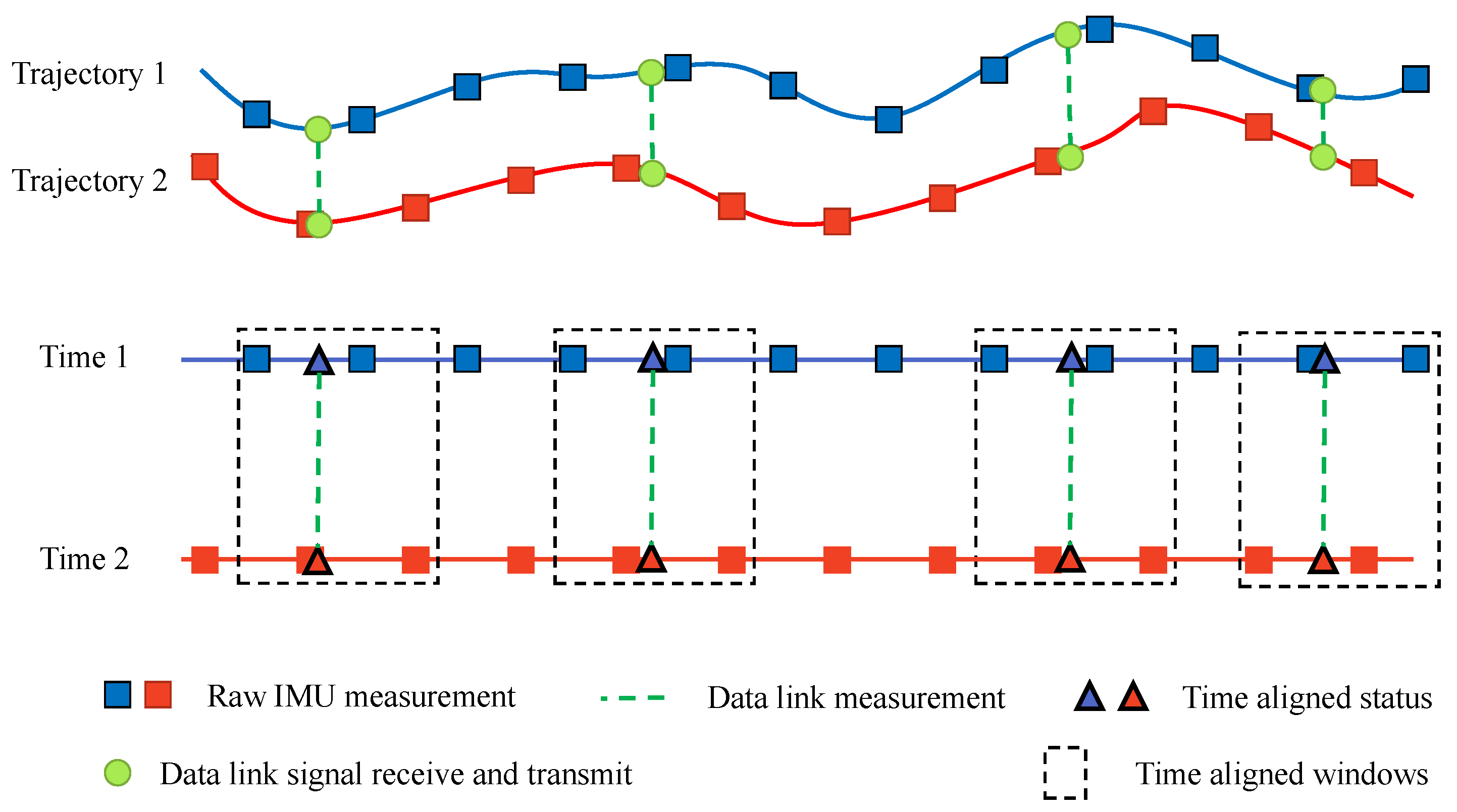
The IMU on the UAV operates at a frequency of 100 Hz, while the data link communication frequency is 30 Hz. Additionally, the IMU sensors on different UAVs within the formation have asynchronous reference times, complicating the synchronization of data from these sensors. To address this issue, a time alignment method based on the data link signal timestamp is employed, as illustrated in Figure 2.

In Figure 2, the square nodes represent the flight states estimated by the inertial navigation integration algorithm, as described in Section 2.4. The circular nodes represent the data link measurements between the two UAVs. The green dashed lines indicate the measurements between the data link equipment pairs, as discussed in Section 2.5, and the dashed box represents the time alignment window, which includes a data link measurement and the two nearest flight states. By interpolating the UAV states of both UAVs within this time window, the state parameters of the UAV, aligned with the data link measurement moment, can be calculated, as shown in the triangular nodes. Specifically, the drone state parameters include both position and orientation. While position data exist in a linear space and can be effectively interpolated using direct linear interpolation, orientation data, represented as rotations, are not continuous in linear space. Instead, they exist on the unit quaternion manifold, where direct linear interpolation can introduce significant errors, particularly for large rotations. Therefore, we employ SLERP, which provides smooth, constant speed interpolation along the shortest path on the quaternion manifold, ensuring the accurate alignment of orientation data, as described in Equations (24)–(26).

$$\begin{array}{c}\hfill f_k={\displaystyle \frac{t_k-t_m}{t_n-t_m}}.\end{array}$$

(24)

$$\begin{array}{c}\hfill cos(\theta )={\mathit{q}}_m\otimes {\mathit{q}}_n.\end{array}$$

(25)

$$\begin{array}{c}\hfill {\mathit{q}}_k={\displaystyle \frac{sin((1-f_k)·\theta )·{\mathit{q}}_m+sin(f_k·\theta )·{\mathit{q}}_n}{sin(\theta )}}.\end{array}$$

(26)

$$\begin{array}{c}\hfill {\mathit{p}}_k={\mathit{p}}_m+f_k·({\mathit{p}}_n-{\mathit{p}}_m).\end{array}$$

(27)

$$\begin{array}{c}\hfill {\mathit{v}}_k={\mathit{v}}_m+f_k·({\mathit{v}}_n-{\mathit{v}}_m).\end{array}$$

(28)

In the interpolation process, $t_k$ represents the time point to be interpolated, while ${\mathit{q}}_k$, ${\mathit{p}}_k$, and ${\mathit{v}}_k$ denote the corresponding UAV state parameters after time alignment. $f_k$ represents the interpolation scale factor, while ⊗ denotes quaternion multiplication. Additionally, $t_m$ and $t_n$ are the timestamps of the inertial navigation estimates before and after the moment $t_k$, respectively. Similarly, ${\mathit{q}}_m$, ${\mathit{q}}_n$, ${\mathit{p}}_m$, ${\mathit{p}}_n$, ${\mathit{v}}_m$, and ${\mathit{v}}_n$ represent the UAV’s state parameters at the timestamp $t_m$ and $t_n$.

Consider UAV a and b flying in formation as an example. The two UAVs exchange their flight state parameters respectively via data link communication. To ensure consistency, each UAV performs time synchronization between its own state parameters and the received flight state parameters of its teammate. Subsequently, the aligned flight state parameters and data link measurements are integrated into the data frame $\mathsf{\chi }=\left\{{\mathit{p}}_a^k,{\mathit{p}}_b^k,{\mathit{q}}_a^k,{\mathit{q}}_b^k,{\mathit{v}}_a^k,{\mathit{v}}_b^k{,}^{a_{\mathcal{N}}}{\mathit{p}}_b^k\right\}$.

To ensure both the diversity of optimization data and the real-time optimization of relative pose estimation, time-aligned data were preselected before the optimization process. The selection of optimization data was based on the diversity of geometric features in the flight trajectories. Specifically, the state parameters after the current alignment were compared with those from the previous alignment. If all parameters of the data frame, except for the position parameters, remained unchanged, it was determined that the UAVs in formation were flying in parallel along a straight line trajectory. In such cases, these data were considered redundant and excluded from subsequent optimization.

2.8. Relative Pose Optimization

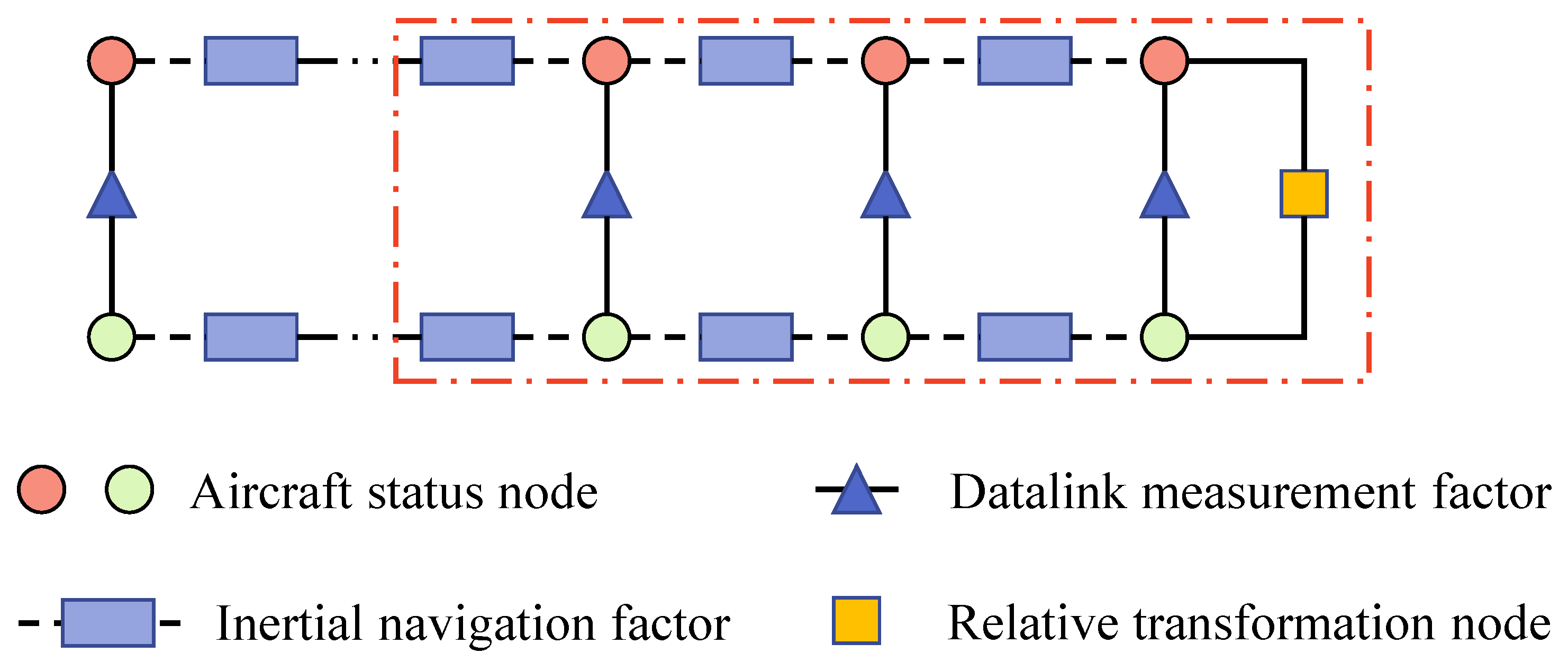
Following data alignment and selection using the method outlined in Section 2.5, the aligned data frames are utilized to construct the relative pose optimization factor graph model, as illustrated in Figure 3. Factor graph optimization is a powerful approach for state estimation that represents the relationships between various measurements and system states as a graph. In this framework, the nodes represent the states of the UAVs, including their positions and orientations, while the edges (factors) represent the constraints provided by sensor measurements, such as inertial data and ranging information. Unlike traditional filtering methods like the Kalman filter, which rely on a first-order, implicit sliding window, factor graph optimization maintains an explicit sliding window, typically encompassing multiple historical states for joint optimization. This approach offers several key advantages: 1. By optimizing multiple frames simultaneously, factor graphs can correct past state estimates when new information becomes available, reducing long-term drift and improving overall consistency. 2. Factor graphs can incorporate a wide range of measurement types and constraints, including nonlinear relationships, making them well-suited for complex multi-UAV scenarios. 3. Unlike recursive, forward-only methods, factor graph optimization allows for the redistribution of errors across the sliding window, providing more accurate state estimation in GNSS-denied or bias-prone environments. This structure provides a robust foundation for accurate relative pose estimation in UAV formations, as it effectively fuses diverse sensor data while mitigating the impact of drift and noise.

In this factor graph model, each node represents the state parameters of a UAV. Specifically, red nodes denote the state parameters of the UAV itself, green nodes correspond to the state parameters of its teammate, and blue rectangular nodes represent inertial navigation factors, which encode the inertial integration constraints between connected state parameter nodes. The blue triangular nodes denote data link measurement factors, capturing the relative measurements between the two UAVs’ state parameters. The yellow square nodes represent the relative pose transformations between the connected UAV state parameters, serving as the variables to be optimized within the factor graph.

To ensure real-time computational efficiency while maintaining an overdetermined equation system for optimization, a sliding window mechanism is employed, indicated by a red dashed box in the figure. The optimization process is constrained to the nodes within this sliding window. The size of the sliding window is determined by balancing the computational resources available and the need for consistent optimization results. Specifically, the window size is influenced by three key factors: 1. Equation Closure: The factor graph must remain well-constrained, requiring that the number of residuals (constraints) exceeds the number of optimization variables. 2. Real-Time Performance: The number of nodes directly affects the dimensionality of the optimization problem. To achieve real-time performance, it is necessary to limit the dimensionality according to the available computational capacity. 3. Optimization Consistency: Including more nodes in the sliding window improves the global consistency of the optimization result. Considering these factors, the sliding window is set to include as many nodes as possible without compromising real-time performance. In this study, the sliding window is set to a time interval of 10 s, encompassing n measurements (where $n>3$), including 300 data frames. Additionally, to mitigate unconvergence issues caused by the long-term drift of inertial navigation integration, the time interval between the first and last frame within the sliding window is constrained.

In Figure 3, each time-aligned data frame, along with the corresponding relative pose transformation node and the associated inertial navigation integration factors, forms a complete closed loop. Each of these closed loops enables the construction of a relative position residual ${\mathit{e}}_p$. Taking the pose residual ${\mathit{e}}_p^{k-i}$ derived from the $(k-i)$th data frame as an example, its computation is given by the following:

$$\begin{array}{c}\hfill {\mathit{e}}_p^{k-i}{=}^{a_{\mathcal{B}}}{\overline{\mathit{p}}}_b^{k-i}{-}^{a_{\mathcal{B}}}{\widehat{\mathit{p}}}_b^{k-i},\end{array}$$

(29)

where ${}_{ }{}^{a_{\mathcal{B}}}\overline{\mathit{p}}_b^{k-i}$ represents the position of UAV b in the data link coordinate system of UAV a at timestamp $k-i$, as measured by the data link. Meanwhile, ${}_{ }{}^{a_{\mathcal{B}}}\widehat{\mathit{p}}_b^{k-i}$ denotes the position of UAV b in the data link coordinate system of UAV a at timestamp $k-i$, as estimated by the inertial navigation system.

The data link system is capable of measuring the position ${}_{ }{}^{a_{\mathcal{N}}}\mathit{p}_b^{k-i}$ of UAV b in the NEU coordinate system of UAV a at timestamp $k-i$. By applying the pose transformation matrix ${\mathit{T}}_{a_{\mathcal{B}},a_{\mathcal{N}}}^{k-i}$, this position can be transformed into the body coordinate system of UAV a, yielding the position ${}_{ }{}^{a_{\mathcal{B}}}\mathit{p}_b^{k-i}$ of UAV b at timestamp $k-i$. The transformation is expressed as follows:

$$\begin{array}{c}\hfill {}_{ }{}^{a_{\mathcal{B}}}\overline{\mathit{p}}_b^{k-i}={\mathit{T}}_{a_{\mathcal{B}},a_{\mathcal{N}}}^{k-i}{·}^{a_{\mathcal{N}}}{\overline{\mathit{p}}}_b^{k-i}.\end{array}$$

(30)

By utilizing the inertial navigation factors and the relative pose nodes involved in the closed loop, the position of UAV b in the body coordinate system of UAV a can be calculated as follows:

$$\begin{array}{c}\hfill {}_{ }{}^{a_{\mathcal{B}}}\widehat{\mathit{p}}_b^{k-i}{=}^{a_{\mathcal{B}}}{\mathit{M}}_{k-i,k}·{\mathit{T}}_{a_{\mathcal{B}},b_{\mathcal{B}}}^k{·}^{b_{\mathcal{B}}}{\mathit{M}}_{k,k-i}{·}^{b_{\mathcal{B}}}{\mathit{p}}_b^{k-i},\end{array}$$

(31)

where ${}_{ }{}^{a_{\mathcal{B}}}\mathit{M}_{k-i,k}^{ }$ represents the transformation matrix from the body coordinate system of UAV a at timestamp k to the body coordinate system of UAV a at timestamp $k-i$, and ${}_{ }{}^{b_{\mathcal{B}}}\mathit{M}_{k,k-i}^{ }$ denotes the transformation matrix from the body coordinate system of UAV b at timestamp $k-i$ to the body coordinate system of UAV b at timestamp k. Additionally, ${\mathit{T}}_{a_{\mathcal{B}},b_{\mathcal{B}}}^k$ represents the relative pose of the body coordinate system of UAV b with respect to the body coordinate system of UAV a at timestamp k. ${}_{ }{}^{b_{\mathcal{B}}}\mathit{p}_b^{k-i}$ represents the position of UAV b in its body coordinate system at timestamp $k-i$. The transformation matrices ${}_{ }{}^{b_{\mathcal{B}}}\mathit{M}_{k,k-i}^{ }$ and ${}_{ }{}^{a_{\mathcal{B}}}\mathit{M}_{k-i,k}^{ }$ can be computed using the transitivity property of inertial data, as follows:

$$\begin{array}{c}\hfill {}_{ }{}^{a_{\mathcal{B}}}\mathit{M}_{k-i,k}^{ }{=}^{a_{\mathcal{B}}}{\mathit{M}}_{k-i,k-i+1}·\cdots {·}^{a_{\mathcal{B}}}{\mathit{M}}_{k-1,k},\end{array}$$

(32)

$$\begin{array}{c}\hfill {}_{ }{}^{b_{\mathcal{B}}}\mathit{M}_{k,k-i}^{ }{=}^{b_{\mathcal{B}}}{\mathit{M}}_{k,k-1}·\cdots {·}^{b_{\mathcal{B}}}{\mathit{M}}_{k-i+1,k-i}.\end{array}$$

(33)

In each closed loop, the inertial factors on one side of the loop can be multiplied to obtain the transformation matrix ${}_{ }{}^{a_{\mathcal{B}}}\mathit{M}_{k-i,k}^{ }$ and ${}_{ }{}^{b_{\mathcal{B}}}\mathit{M}_{k,k-i}^{ }$, which describes the transform in the body coordinate system from timestamp $k-i$ to timestamp k. Inertial navigation can compute the position and orientation of the UAV’s body system in its navigation coordinate system at continuous time intervals. By using the ECEF coordinate system as an intermediary, the transformation matrix ${}_{ }{}^{b_{\mathcal{B}}}\mathit{M}_{k-i+1,k-i}^{ }$ and ${}_{ }{}^{a_{\mathcal{B}}}\mathit{M}_{k-i,k-i+1}^{ }$ corresponding to each inertial factor can be derived. The individual transformation matrices for ${}_{ }{}^{a_{\mathcal{B}}}\mathit{M}_{k-1,k}^{ }$ and ${}_{ }{}^{b_{\mathcal{B}}}\mathit{M}_{k,k-1}^{ }$ are computed as follows:

$$\begin{array}{c}\hfill {}_{ }{}^{a_{\mathcal{B}}}\mathit{M}_{k-1,k}^{ }={\mathit{T}}_{a_{\mathcal{B}},a_{\mathcal{N}}}^{k-1}·{\mathit{T}}_{a_{\mathcal{N}},\mathcal{E}}^{k-1}·{\mathit{T}}_{\mathcal{E},a_{\mathcal{N}}}^k·{\mathit{T}}_{a_{\mathcal{N}},a_{\mathcal{B}}}^k,\end{array}$$

(34)

$$\begin{array}{c}\hfill {}_{ }{}^{b_{\mathcal{B}}}\mathit{M}_{k,k-1}^{ }={\mathit{T}}_{b_{\mathcal{B}},b_{\mathcal{N}}}^k·{\mathit{T}}_{b_{\mathcal{N}},\mathcal{E}}^k·{\mathit{T}}_{\mathcal{E},b_{\mathcal{N}}}^{k-1}·{\mathit{T}}_{b_{\mathcal{N}},b_{\mathcal{B}}}^{k-1}.\end{array}$$

(35)

where ${\mathit{T}}_{b_{\mathcal{B}},b_{\mathcal{N}}}^k$ denotes the transformation matrix from the east-north-up coordinate system of UAV b at timestamp k to the body coordinate system. ${\mathit{T}}_{b_{\mathcal{N}},\mathcal{E}}^k$ represents the transformation matrix from the geocentric coordinate system to the east-north-up coordinate system of UAV b at timestamp k. ${\mathit{T}}_{\mathcal{E},b_{\mathcal{N}}}^{k-i}$ signifies the transformation matrix from the north-east-down coordinate system of UAV b at timestamp $k-i$ to the geocentric coordinate system. ${\mathit{T}}_{b_{\mathcal{N}},b_{\mathcal{B}}}^{k-i}$ represents the transformation matrix from the body coordinate system to the north-east-down coordinate system of UAV b at timestamp $k-i$.

As illustrated in Figure 3, each closed loop, comprising a data frame and a relative transformation node, can construct a relative pose residual. By integrating the n relative pose residuals within the sliding window, the optimization equation for refining the relative transformation node is formulated as follows:

$$\begin{array}{c}\hfill {\mathit{x}}^{*}=arg\underset{\mathit{x}}{min}\sum _{i=0}^n{\displaystyle \frac{1}{2}}{({\mathit{e}}_p^{k-i})}^T{\mathit{W}}^{k-i}{\mathit{e}}_p^{k-i},\end{array}$$

(36)

where ${\mathit{W}}^{k-i}$ represents the information matrix of the relative position error at the $k-ith$ instance. The cost function ${\mathit{e}}_p^{k-i}$ corresponds to the relative position residual as described in Equation (29). The optimization variable x consists of the relative pose between UAVs, denoted by ${\mathit{T}}_{a_{\mathcal{B}},b_{\mathcal{B}}}^k$. By transforming the rotation matrix ${\mathit{R}}_{a_{\mathcal{B}},b_{\mathcal{B}}}^k$ in ${\mathit{T}}_{a_{\mathcal{B}},b_{\mathcal{B}}}^k$ into its corresponding Lie algebra ${\mathsf{\varphi }}_{a_{\mathcal{B}},b_{\mathcal{B}}}^k$, the optimization variable can be expressed as ${\mathit{x}}_{a_{\mathcal{B}},b_{\mathcal{B}}}^k={[{{\mathsf{\varphi }}_{a_{\mathcal{B}},b_{\mathcal{B}}}^k}^T,{{\mathit{t}}_{a_{\mathcal{B}},b_{\mathcal{B}}}^k}^T]}^T$. Within the sliding window framework, only a single type of residual is considered. Given that the time interval of the optimized sliding window is relatively short, the drift of the inertial navigation factors contributing to the residual can be neglected. As a result, it is reasonable to assume that the confidence level of each residual is equivalent, leading to the assignment of ${\mathit{W}}^{k-i}=\mathit{I}$.

During the optimization process, the Jacobian matrix of ${\mathit{e}}_p^{k-i}$ with respect to ${\mathit{x}}_{a_{\mathcal{B}},b_{\mathcal{B}}}^k$ is derived analytically. The relationship between ${\mathit{e}}_p^{k-i}$ and ${\mathit{x}}_{a_{\mathcal{B}},b_{\mathcal{B}}}^k$ is established as follows:

$$\begin{array}{cc}\hfill {\mathit{e}}_p^{k-i}=& {\mathit{T}}_{a_{\mathcal{B}},a_{\mathcal{N}}}^{k-i}{·}^{a_{\mathcal{N}}}{\mathit{p}}_b^{k-i}{-}^{a_{\mathcal{B}}}{\mathit{M}}_k^{k-i}·{\mathit{T}}_{a_{\mathcal{B}},b_{\mathcal{B}}}^k{·}^{b_{\mathcal{B}}}{\mathit{M}}_{k-i}^k{·}^{b_{\mathcal{B}}}{\mathit{p}}_b^{k-i}.\hfill \end{array}$$

(37)

The multiplication of ${\mathit{T}}_{a_{\mathcal{B}},b_{\mathcal{B}}}^k$ is equivalent to first performing a rotational transformation with the Lie group corresponding to ${\mathsf{\varphi }}_{a_{\mathcal{B}},b_{\mathcal{B}}}^k$, and then linearly adding the translation ${\mathit{t}}_{a_{\mathcal{B}},b_{\mathcal{B}}}^k$. Therefore, the differentiation can be carried out separately for ${\mathsf{\varphi }}_{a_{\mathcal{B}},b_{\mathcal{B}}}^k$ and ${\mathit{t}}_{a_{\mathcal{B}},b_{\mathcal{B}}}^k$. The corresponding Jacobian matrix ${\mathit{J}}_{a_{\mathcal{B}},b_{\mathcal{B}}}^{k-i}$ can be computed as follows:

$$\begin{array}{cc}\hfill {\mathit{J}}_{a_{\mathcal{B}},b_{\mathcal{B}}}^{k-i}& ={\displaystyle \frac{\partial {\mathit{e}}_p^{k-i}}{\partial {\mathit{x}}_{a_{\mathcal{B}},b_{\mathcal{B}}}^k}}={\displaystyle \frac{\partial {\mathit{e}}_p^{k-i}}{\partial \left[\begin{array}{c}\begin{array}{c}\delta {\mathsf{\varphi }}_{a_{\mathcal{B}},b_{\mathcal{B}}}^k\\ \delta {\mathit{t}}_{a_{\mathcal{B}},b_{\mathcal{B}}}^k\end{array}\end{array}\right]}}\hfill \\ \hfill & ={\displaystyle \frac{\partial ({-}^{a_{\mathcal{B}}}{\mathit{M}}_k^{k-i}·{\mathit{T}}_{a_{\mathcal{B}},b_{\mathcal{B}}}^k{·}^{b_{\mathcal{B}}}{\mathit{M}}_{k-i}^k{·}^{b_{\mathcal{B}}}{\mathit{p}}_b^{k-i})}{\partial \left[\begin{array}{c}\begin{array}{c}\delta {\mathsf{\varphi }}_{a_{\mathcal{B}},b_{\mathcal{B}}}^k\\ \delta {\mathit{t}}_{a_{\mathcal{B}},b_{\mathcal{B}}}^k\end{array}\end{array}\right]}}\hfill \\ \hfill & ={-}^{a_{\mathcal{B}}}{\mathit{M}}_k^{k-i}{\displaystyle \frac{\partial ({\mathit{R}}_{a_{\mathcal{B}},b_{\mathcal{B}}}^k·{}_{ }{}^{b_{\mathcal{B}}}\mathit{M}_{k-i}^k·{}_{ }{}^{b_{\mathcal{B}}}\mathit{p}_b^{k-i}+\delta {\mathit{t}}_{a_{\mathcal{B}},b_{\mathcal{B}}}^k)}{\partial \left[\begin{array}{c}\begin{array}{c}\delta {\mathsf{\varphi }}_{a_{\mathcal{B}},b_{\mathcal{B}}}^k\\ \delta {\mathit{t}}_{a_{\mathcal{B}},b_{\mathcal{B}}}^k\end{array}\end{array}\right]}}.\hfill \end{array}$$

(38)

Using the left perturbation model approach, the partial derivative of ${\mathit{e}}_p^{k-i}$ with respect to ${\mathsf{\varphi }}_{a_{\mathcal{B}},b_{\mathcal{B}}}^k$ can be calculated as follows:

$$\begin{array}{c}\hfill {\displaystyle \frac{\partial ({\mathit{R}}_{a_{\mathcal{B}},b_{\mathcal{B}}}^k{·}^{b_{\mathcal{B}}}{\mathit{M}}_{k-i}^k{·}^{b_{\mathcal{B}}}{\mathit{p}}_b^{k-i})}{\partial [{\mathsf{\varphi }}_{a_{\mathcal{B}},b_{\mathcal{B}}}^k]}}=-{({\mathit{R}}_{a_{\mathcal{B}},b_{\mathcal{B}}}^k{·}^{b_{\mathcal{B}}}{\mathit{M}}_{k-i}^k{·}^{b_{\mathcal{B}}}{\mathit{p}}_b^{k-i})}^{\wedge }.\end{array}$$

(39)

The partial derivative of ${\mathit{e}}_p^{k-i}$ with respect to ${\mathit{t}}_{a_{\mathcal{B}},b_{\mathcal{B}}}^k$ is as follows:

$$\begin{array}{c}\hfill {\displaystyle \frac{\partial ({\mathit{R}}_{a_{\mathcal{B}},b_{\mathcal{B}}}^k·{}_{ }{}^{b_{\mathcal{B}}}\mathit{M}_{k-i}^k·{}_{ }{}^{b_{\mathcal{B}}}\mathit{p}_b^{k-i})+{\mathit{t}}_{a_{\mathcal{B}},b_{\mathcal{B}}}^k}{\partial {\mathit{t}}_{a_{\mathcal{B}},b_{\mathcal{B}}}^k}}={\mathit{I}}_{3\times 3}.\end{array}$$

(40)

Combining the partial derivatives obtained for ${\mathsf{\varphi }}_{a_{\mathcal{B}},b_{\mathcal{B}}}^k$ and ${\mathit{t}}_{a_{\mathcal{B}},b_{\mathcal{B}}}^k$, the Jacobian matrix ${\mathit{J}}_{a_{\mathcal{B}},b_{\mathcal{B}}}^{k-i}$ of ${\mathit{e}}_p^{k-i}$ with respect to ${\mathit{x}}_{a_{\mathcal{B}},b_{\mathcal{B}}}^k$ can be derived.

$$\begin{array}{cc}\hfill {\mathit{J}}_{a_{\mathcal{B}},b_{\mathcal{B}}}^{k-i}=& [{-}^{a_{\mathcal{B}}}{\mathit{M}}_k^{k-i}·{({\mathit{R}}_{a_{\mathcal{B}},b_{\mathcal{B}}}^k{·}^{b_{\mathcal{B}}}{\mathit{M}}_{k-i}^k{·}^{b_{\mathcal{B}}}{\mathit{p}}_b^{k-i})}^{\wedge },{-}^{a_{\mathcal{B}}}{\mathit{M}}_k^{k-i}].\hfill \end{array}$$

(41)

The factor graph model as depicted in Figure 3 is solved by the open-source C++ library Ceres. The Levenberg–Marquardt method is chosen to solve the optimization equations, with the Huber function selected as the robust kernel function.

3. Simulation and Real World Experimental Analysis

To validate the effectiveness and accuracy of the proposed method in relative localization, simulation tests were designed, and real-world experiments were conducted in typical task scenarios.

3.1. Simulation Experimental Analysis

In the simulation, we modeled an IMU based on the specifications of the ADIS16470 IMU, which is widely used in drone applications. The simulated accelerometer and gyroscope data were generated using a noise model consistent with the sensor datasheet. The simulated IMU state parameters are shown in

Table 1. Characteristic parameters of the IMU.

Sensor	Frequency (Hz)	Bias	Random Walk Noise
Accelerometer	100	(5, 5, 5) (${10}^{-5}$ $\mathrm{m}/{\mathrm{s}}^2$)	(3, 3, 3) (${10}^{-2}$ m/s/$\sqrt{\mathrm{h}}$)
Gyroscope	100	(6, 6, 6) (deg/h)	(2.5, 2.5, 2.5) (${10}^{-1}$ deg/$\sqrt{\mathrm{h}}$)

and

Table 2. Characteristic parameters of the data link.

Frequency (Hz)	Bias of Distance (m)	Distance Error (m)
100	200	50

. Drawing from actual flight missions, flight trajectories for the UAV are devised. The state parameters of the drone in the positioning coordinate system (ENU) are calibrated before flight. The initial states of drone a and drone b are detailed in

Table 3. Aircraft initial state parameters.

UAV	Longitude (deg)	Latitude (deg)	Altitude (m)	Yaw (deg)	Pitch (deg)	Roll (deg)
a	120.0	32.0	100	0.0	0.0	0.0
b	120.0	32.0	600	0.0	0.0	0.0

, and the flight state variables are shown in

Table 4. Flight parameter table of the aircraft in the formation during the simulation experiment.

UAV a		UAV b		During Time
Yaw (deg)	Upwards Speed (m/s)	Yaw (deg)	Northbound Speed (m/s)	Complete Time (s)
0	20	90	20	40
180	20	90	20	40
180	20	270	20	80
0	20	−90	20	80
180	20	−270	20	40
180	20	−270	20	40
0	20	−90	20	80

. In Table 4, the state quantities reflect the states achieved after the specified time, and the flight state parameters evolve in accordance with the dynamic characteristics of the UAV during flight.

The simulation program generates synthetic acceleration and angular velocity data corresponding to the predefined UAV trajectories. By employing the inertial navigation integration algorithm described in Section 2.4, the UAV’s state parameters are computed at each time step. A comparison between the estimated and designed flight trajectories is presented in Figure 4. The results indicate that the estimated trajectories closely align with the designed ones, demonstrating the high accuracy of the inertial navigation algorithm in pose estimation. However, as flight time progresses, drift gradually accumulates in the estimated trajectories, with more pronounced deviations occurring in the final segment. This phenomenon is consistent with the characteristic long-term pose drift inherent in inertial navigation estimation. Nevertheless, over short durations, the estimated trajectory remains closely aligned with the actual flight path, confirming the algorithm’s effectiveness in accurately estimating the vehicle’s flight state parameters. Furthermore, this ensures the provision of precise pose constraints for the frames within the sliding window of the factor graph.

Based on the position of each UAV in its navigation coordinate systems, the relative distance, azimuth angle, and altitude angle between the UAV can be calculated as follows:

$$\begin{array}{cc}\hfill d_k& =({({\mathit{T}}_{\mathcal{E},a_{\mathcal{N}}}^k{·}^{a_{\mathcal{N}}}{\mathit{p}}_a^k-{\mathit{T}}_{\mathcal{E},b_{\mathcal{N}}}^k{·}^{b_{\mathcal{N}}}{\mathit{p}}_b^k)}^T·\hfill \\ \hfill & ({\mathit{T}}_{\mathcal{E},a_{\mathcal{N}}}^k{·}^{a_{\mathcal{N}}}{\mathit{p}}_a^k-{\mathit{T}}_{\mathcal{E},b_{\mathcal{N}}}^k{·}^{b_{\mathcal{N}}}{\mathit{p}}_b^k){)}^{{\displaystyle \frac{1}{2}}},\hfill \end{array}$$

(42)

$$\begin{array}{c}\hfill {}_{ }{}^{a_{\mathcal{N}}}\mathit{p}_b^k={\mathit{T}}_{a_{\mathcal{N}},\mathcal{E}}^k{·}^{\mathcal{E}}{\mathit{p}}_b^k,\end{array}$$

(43)

$$\begin{array}{c}\hfill {\gamma }_k=arcsin({\displaystyle \frac{{{[}^{a_{\mathcal{N}}{\mathit{p}}_b^k}]}_z}{d_k}}),\end{array}$$

(44)

$$\begin{array}{c}\hfill {\alpha }_k=arcsin({\displaystyle \frac{{{[}^{a_{\mathcal{N}}}{\mathit{p}}_b^k]}_x}{d_k·cos({\gamma }_k)}}),\end{array}$$

(45)

where ${\mathit{T}}_{\mathcal{E},a_{\mathcal{N}}}^k$ and ${\mathit{T}}_{\mathcal{E},b_{\mathcal{N}}}^k$ denote the transformation matrices from the navigation coordinate systems of UAVs a and b, respectively, to the ECEF coordinate system at timestamp k. ${}_{ }{}^{a_{\mathcal{N}}}\mathit{p}_a^k$ and ${}_{ }{}^{b_{\mathcal{N}}}\mathit{p}_b^k$ represent the positions of UAV a and b in their respective navigation coordinate systems at timestamp k. $d_k$ signifies the distance measured between UAV a and b at timestamp k. ${}_{ }{}^{a_{\mathcal{N}}}\mathit{p}_b^k$ and ${}_{ }{}^{\mathcal{E}}\mathit{p}_b^k$ correspond to the positions of UAV b relative to UAV a in the ENU coordinate system of UAV a at timestamp k and in the ECEF coordinate system at timestamp k. ${\alpha }_k$ denotes the elevation angle measured by the data link at timestamp k, while ${\gamma }_k$ represents the azimuth angle measured by the data link at timestamp k.

The simulation results of the data link measurements can be calculated based on the noise described in Table 2 and the ${\alpha }_k$, ${\gamma }_k$, $d_k$. The simulation of distance, azimuth angle, and altitude angle are depicted in Figure 5 and Figure 6, respectively.

The current fusion method of data link and inertial navigation information primarily employs the Kalman filtering technique. We designed a motion model based on the inertial navigation method and utilized the data link measurement information as the observations to update the relative pose during flight. To validate the accuracy of the proposed algorithm, relative pose calculations are performed using Kalman filtering, the pose graph optimization method proposed in Section 2.8, and the data link measurement method, respectively. The calculated results are compared with the simulated truth to obtain the errors in relative distance, azimuth angle, and altitude angle, as illustrated in Figure 7, Figure 8 and Figure 9.

As illustrated in Figure 7, the sliding window is configured with a size of 300, and error computations commence from the 10th second onward. The error characteristics of the data link measurements conform to the designed simulation parameters, exhibiting a bias of 200 and a variance of 200 for Gaussian white noise. While the Kalman filtering algorithm effectively attenuates errors arising from Gaussian white noise in data link measurements, it is unable to compensate for errors introduced by bias. In contrast, the factor graph optimization method not only corrects errors caused by bias but also effectively mitigates the influence of Gaussian white noise. Unlike the Kalman filtering algorithm, which operates on a per-measurement basis, the proposed method in Section 2.8 leverages data from the entire sliding window, incorporating 600 nodes in the optimization process. By integrating inertial navigation constraints between adjacent nodes and data link measurement constraints between node pairs within the sliding window, the proposed approach significantly reduces errors introduced by white noise. Furthermore, the continuity constraint imposed on node motion within the sliding window alleviates discontinuities in distance measurements caused by data link bias at crossover points where UAV a and UAV b intersect. As a result, the method effectively eliminates errors stemming from data link measurement bias, ensuring improved accuracy in position estimation.

As illustrated in Figure 8, the altitude angle errors obtained through factor graph optimization, Kalman filtering, and data link measurements remain minimal. This is primarily due to the smooth and regular variations in altitude angles between UAVs in the designed trajectory. Consequently, both the Kalman filter and factor graph optimization methods demonstrate comparable accuracy in mitigating errors induced by data link measurement noise.

As depicted in Figure 9, spikes are evident in the azimuth angle measurement errors. These spikes stem from the presence of crossover points between UAV a and b in the horizontal direction during flight. The conflicting relative position vectors before and after the crossover point contribute to imprecise solutions. Kalman filtering adeptly reduces the spikes by integrating the current measurement with the previous state using the Kalman gain. The factor graph optimization leverages the transitivity of inertial navigation constraints between all nodes in the sliding window and the consistency of azimuth angle changes effectively eliminates the spikes and mitigates errors induced by white noise.

The Root Mean Square Error (RMSE) serves as a standard quantitative metric for evaluating the accuracy of relative position between UAVs estimated by data chain measurement, Kalman filtering, and factor graph optimization. The RMSE calculation formula is as follows:

$$\begin{array}{c}\hfill RMS{E}_x=\sqrt{{\displaystyle \frac{1}{n}}\sum _{i=0}^n{({\mathit{x}}_{est}-{\mathit{x}}_{true})}^2},\end{array}$$

(46)

where n is the total number of samples, ${\mathit{x}}_{\mathrm{true}}$ is the true value of the $i\text{-}\mathrm{th}$ sample, and ${\mathit{x}}_{\mathrm{est}}$ is the estimated value of the $i\text{-}\mathrm{th}$ sample. The RMSE values for different algorithms estimating poses are presented in

Table 5. The RMSE of relative positions between UAVs.

Method	Distance (m)	Altitude Angle (deg)	Azimuth Angle (deg)
Data link measurement error	251.6	0.015	0.017
Filter error	233.4	0.012	0.015
Graph optimizer error	58.7	0.011	0.012

.

In Table 5, it is observed that the measurement errors from the data link are the highest among all methods. The filtering method reduces distance errors by $11\%$, altitude angle errors by $20\%$, and azimuth angle errors by $12\%$. However, the factor graph optimization method significantly outperforms the filtering method, reducing distance errors by $77\%$, altitude angle errors by $26\%$, and azimuth angle errors by $29\%$. The dominant source of distance errors is attributed to bias terms and filtering methods cannot eliminate the error generated by bias; hence, the reduction in distance errors is relatively modest for the filtering method. Conversely, the proposed graph optimization method leverages the specific characteristics of flight trajectory intersection points to eliminate part of the distance error induced by bias, resulting in a substantial decrease in distance errors. Since the trajectories of the two UAVs exhibit minimal variations in the altitude direction, with strong constraints from inertial navigation, both filtering and optimization methods demonstrate significant reductions in altitude angle measurement errors. As azimuth angle measurements are highly accurate and exhibit considerable variations during flight, both filtering and factor graph optimization methods can only address errors caused by white noise. However, the graph optimization involves more flight state information, leading to higher accuracy in azimuth angle measurement.

The simulation results evidence the efficacy of the proposed method in typical mission scenarios. By leveraging historical measurement data to construct a factor graph with additional constraint terms, the method adeptly mitigates measurement biases and diminishes errors induced by white noise. Consequently, it substantially enhances the accuracy of relative pose estimation.

3.2. Real World Experimental Verification

In a representative combat environment, actual flight tests were conducted using two fixed-wing UAVs to evaluate the performance of the proposed cooperative positioning algorithm. Each UAV was equipped with a high-precision inertial measurement unit (IMU) for state estimation. Specifically, the HG1930 IMU sensor was selected for this experiment, with its key performance parameters provided in

Table 6. Characteristic parameters of the IMU.

Sensor	Frequency (Hz)	Bias	Random Walk Noise
Accelerometer	500	(5, 5, 5) (${10}^{-5}$ $\mathrm{m}/{\mathrm{s}}^2$)	(3, 3, 3) (${10}^{-2}$ m/s/$\sqrt{\mathrm{h}}$)
Gyroscope	500	(1, 1, 1) (${10}^{-2}\mathrm{deg}/\mathrm{h}$)	(5, 5, 5) (${10}^{-3}$ deg/$\sqrt{\mathrm{h}}$)

. To enable inter-UAV communication and relative positioning, each UAV was also equipped with a FreeWave ZumLink data link device. These devices support distance and angle measurements between UAVs in the formation, with data links installed in six directions to provide comprehensive relative state information. The relevant specifications of the data link system are detailed in

Table 7. Characteristic parameters of the data link.

Frequency (Hz)	Bias of Distance (m)	Distance Error (m)
10	180	60

. For absolute positioning, each UAV was equipped with a dual-frequency GNSS receiver, providing centimeter-level accuracy for ground truth data, which was used to validate the performance of the proposed algorithm. The pre-flight state parameters of each UAV, including initial position and orientation, are presented in

Table 8. Aircraft initial state parameters.

UAV	Longitude (deg)	Latitude (deg)	Altitude (m)	Yaw (deg)	Pitch (deg)	Roll (deg)
a	120.0	32.0	283	0.0	0.0	0.0
b	120.0	32.0	283	0.0	0.0	0.0

. The onboard processing system for each UAV featured a six-core 3 GHz CPU, capable of executing the factor graph optimization algorithm within a sliding window of 200 nodes. This configuration achieved a sub-millisecond computation cycle, approximately 1 millisecond per optimization iteration, demonstrating that the system has sufficient computational capacity to maintain real-time relative state estimation within the UAV formation. Prior to the experimental deployment, each UAV remained stationary at the airport to acquire GNSS signals for precise initial position determination. A coordinate system calibration procedure was then performed, aligning each UAV to a common positioning coordinate system (ENU) to establish accurate initial state parameters, ensuring consistent formation control and relative pose estimation during flight.

The trajectories shown in Figure 10 represent the partial flight paths of the two UAVs during the experiment. The IMU sensor and data link measurement data collected from both UAVs exhibited discrepancies in system time, resulting in temporal misalignment. To address this issue, the time alignment method described in Section 2.7 was applied to synchronize data obtained from different sensors. Figure 11 presents a comparison between the inter-UAV distances computed using the INS + GNSS integrated navigation method and the corresponding data link measurement values after time alignment.

In Figure 11, following time alignment, both the calculated distances and data link measurement values demonstrate synchronous temporal fluctuations. Upon closer examination of the graph’s magnified section, it is evident that the calculated data and measured values attain peak and trough points simultaneously. This synchronization indicate the effectiveness of the time alignment method elucidated in Section 2.7 in resolving the challenge posed by disparate sensor system times within the formation, thereby ensuring temporal coherence across measurements.

The relative position results computed using the INS+GNSS integrated navigation method are regarded as ground truth values. Equations (43)–(46) are employed to calculate the reference values for relative positions between UAVs. Following this, the proposed factor graph optimization, Kalman filtering, and data link measurement methods are utilized to compute the relative positions between UAVs, respectively. The comparison errors between the computed results and the reference values are meticulously presented in Figure 12, Figure 13 and Figure 14.

As depicted in Figure 12, when UAV 1 and UAV 2 intersect in the flight plane shown in Figure 10, a sudden change occurs in the measured distance due to occlusion by the UAV body data link receiver equipment, resulting in a spike in measurement error as shown in Figure 12. The curve of filtering error in the figure is close to the data link measurement error, with the error at the spike of the filtering method being lower than the data link measurement error. The filtering algorithm, by incorporating the previous measurement values, effectively mitigates the spike in error caused by noise. The mean distance error of the factor graph optimization approaches zero in the figure, but its dispersion is greater than that of the data link measurement error and filtering error. The graph optimization method utilizes all measurement data within the sliding window, enabling it to estimate the bias in distance measurement and eliminate spikes during the equipment replacement process. However, the presence of sudden changes in distance measurement within the sliding window affects the estimated values, leading to increased dispersion in the optimization results.

The altitude angle error, as illustrated in Figure 13, displays a slight bias in the data link measured values and a measurement error approximately conforming to a Gaussian distribution with a mean of 0.005 radians. The error distribution resulting from the filtering process closely resembles the measurement error distribution, with the filtering algorithm effectively reducing the standard deviation of the error distribution and thereby enhancing the accuracy of the altitude angle estimation. Conversely, the error derived from the factor graph optimization method demonstrates a Gaussian distribution with a mean of 0 and a significantly diminished standard deviation. This outcome can be attributed to the ability of factor graph optimization to mitigate bias terms while benefiting from the consistent altitude maintained by UAV 2. The stability in altitude leads to minimal error in the elevation estimated by the inertial navigation system, thereby enabling precise altitude angle estimation within the constraints imposed by the inertial navigation system.

As illustrated in Figure 14, the distribution of azimuth errors exhibits similarity when UAV 1 is positioned on one side of UAV 2’s plane during the experiment. When the flight paths of the UAV intersect, the error distribution undergoes alteration. Furthermore, when flying on the same side, the error of data link measurement distribution closely approximates a Gaussian distribution. The variability observed in the error of the filter method closely matches that of the data link measurement error, and the standard deviation of the filter method error is smaller than that of the data link measurement error. The change observed in the graph optimization method error aligns with that of the data link measurement error, and while the standard deviation of the graph optimization error is smaller than that of the data link measurement error, it is slightly larger than that of the filter method error.

The RMSE is used to assess the precision of the proposed method, the filtering algorithm, and the data chain measurement for the relative positions between UAVs. The results are presented in Table 7.

In

Table 9. The RMSE of relative positions between UAVs.

Mehod	Distance (m)	Altitude Angle (deg)	Azimuth Angle (deg)
Data link measurement error	181.4	0.007	0.005
Fliter error	175.6	0.005	0.003
Graph optimizer error	42.7	0.001	0.003

, it is evident that the data link measurement exhibits the highest errors. The filtering method reduces the distance error by $4\%$, the elevation angle error by $28\%$, and the azimuth angle error by $40\%$ compared to the measurements. The proposed graph optimization method significantly reduces the distance error by $76\%$, the elevation angle error by $83\%$, and the azimuth angle error by $40\%$ compared to the measurements. During the experiment, the data link ranging error is attributed to both bias and noise terms. The filtering method is unable to address bias and only handles noise, resulting in a minor improvement in distance error precision, given the relatively small standard deviation of ranging noise. Conversely, the optimization method leverages historical measurements to mitigate bias, but the influence of bias extends to other related measurements, increasing the standard deviation of error distribution. However, the bias impact dominates the error, resulting in a substantial reduction in error after optimization in the proposed method. When the second UAV flies at the same altitude, the inertial navigation estimation algorithm provides accurate altitude values. Moreover, the graph employs more nodes for relative pose optimization, leading to lower elevation angle optimization errors compared to filtering and measurement errors. As the data link provides high precision in azimuth angle measurements and significant azimuth angle variations occur during flight, both filtering and optimization methods offer minor improvements in azimuth angle measurement precision.

The experimental findings demonstrate the effectiveness of the proposed inertial navigation method in Section 2.4 and the time alignment technique in Section 2.7 in generating highly accurate inertial navigation poses and data link measurement information. Based on historical measurement data and utilizing the relative position estimation method from Section 2.8, a higher accuracy relative position between UAVs is achieved. Compared with the results of the filter method and data link measured, the graph optimization method proposed in the article can effectively mitigate biases inherent in data link measurements and improve the accuracy of relative position between UAVs.

4. Conclusions

This paper introduces a novel method for the cooperative positioning of UAV formations, leveraging inertial navigation and data link measurements. By integrating measurements from inertial sensors and data link ranging and angle measurements, the precise estimation of relative poses between UAVs within the formation is achieved. The proposed algorithm establishes a factor graph to estimate relative poses based on historical measurements from both inertial navigation and data link sources. Through graph optimization, accurate relative poses between UAVs are derived. The sliding window method based on short-time measurements effectively addresses prolonged inertial navigation drift issues and utilizes more measurement nodes to build a graph model. Additionally, the proposed time alignment method resolves inconsistencies in sensor system time. Spherical linear interpolation is employed to handle rotation interpolation challenges, while motion models are utilized to address short-term occlusion and measurement failure issues in data link measurements. Simulation and experimental results show that the proposed relative positioning method outperforms data link measurements and traditional filtering methods in accuracy, enabling the real-time accurate estimation of the relative position between UAVs in the formation. However, the proposed method also has certain limitations. For instance, it assumes relatively stable flight dynamics and reliable communication between UAVs, which may not always be achievable in highly dynamic or complex environments. Additionally, the performance of the algorithm can be affected by sensor noise, measurement delays, and communication latency. In cases where the UAV formation undergoes rapid maneuvering or experiences significant external disturbances, the accuracy of relative pose estimation may degrade. For future work, we plan to enhance the robustness of the proposed method under challenging flight conditions. This includes exploring adaptive sliding window strategies, integrating more diverse sensor modalities, and investigating the potential of machine learning approaches, such as time series models, Transformer architectures, and reinforcement learning, to complement the factor graph framework. These methods can better capture the complex temporal dependencies in inertial data and data link measurements, potentially improving the accuracy and robustness of relative pose estimation in dynamic flight environments.

References

1. Wen, L.; Zhen, Z.; Tao, C.; Ding, J. Distributed Cooperative Strategy of UAV Swarm Without Speed Measurement Under Saturation Attack Mission. IEEE Trans. Aerosp. Electron. Syst. 2024, 60, 4518–4529. [Google Scholar] [CrossRef]
2. Zhao, X.; Yang, R.; Zhong, L.; Hou, Z. Multi-UAV path planning and following based on multi-agent reinforcement learning. Drones 2024, 8, 18. [Google Scholar] [CrossRef]
3. Li, N.; Wang, H.; Luo, Q.; Zheng, W. Distributed formation control for multiple quadrotor uavs based on distributed estimator and singular perturbation system. Int. J. Control Autom. Syst. 2024, 22, 1349–1359. [Google Scholar] [CrossRef]
4. Ding, Y.; Kuang, M.; Shi, H.; Gao, J. Multi-UAV Cooperative Target Assignment Method Based on Reinforcement Learning. Drones 2024, 8, 562. [Google Scholar] [CrossRef]
5. Lusk, P.C.; Cai, X.; Wadhwania, S.; Paris, A.; Fathian, K.; How, J.P. A distributed pipeline for scalable, deconflicted formation flying. IEEE Robot. Autom. Lett. 2020, 5, 5213–5220. [Google Scholar] [CrossRef]
6. Lee, E.; Son, J.; Park, S.Y. Relative navigation technique with constrained GNSS data for formation-flying CubeSat mission, CANYVAL-C. Navig. J. Inst. Navig. 2021, 68, 559–575. [Google Scholar] [CrossRef]
7. Gu, S.; Dai, C.; Fang, W.; Zheng, F.; Wang, Y.; Zhang, Q.; Lou, Y.; Niu, X. Multi-GNSS PPP/INS tightly coupled integration with atmospheric augmentation and its application in urban vehicle navigation. J. Geod. 2021, 95, 64. [Google Scholar] [CrossRef]
8. Zhu, H.; Yao, Y.; Ma, X.; Zhang, Q. Tightly coupled multi-frequency PPP-RTK/INS integration model and its application in an urban environment. Geo-Spat. Inf. Sci. 2024, 27, 1685–1699. [Google Scholar] [CrossRef]
9. Geragersian, P.; Petrunin, I.; Guo, W.; Grech, R. An INS/GNSS fusion architecture in GNSS denied environment using gated recurrent unit. In Proceedings of the AIAA SCITECH 2022 Forum, San Diego, CA, USA, 3–7 January 2022; p. 1759. [Google Scholar]
10. Li, J.; Yang, G.; Cai, Q.; Niu, H.; Li, J. Cooperative navigation for UAVs in GNSS-denied area based on optimized belief propagation. Measurement 2022, 192, 110797. [Google Scholar] [CrossRef]
11. Causa, F.; Fasano, G. Improving navigation in GNSS-challenging environments: Multi-UAS cooperation and generalized dilution of precision. IEEE Trans. Aerosp. Electron. Syst. 2020, 57, 1462–1479. [Google Scholar] [CrossRef]
12. Faigl, J.; Krajník, T.; Chudoba, J.; Přeučil, L.; Saska, M. Low-cost embedded system for relative localization in robotic swarms. In Proceedings of the 2013 IEEE International Conference on Robotics and Automation, Karlsruhe, Germany, 6–10 May 2013; pp. 993–998. [Google Scholar]
13. He, Y.; Guo, H.; Li, X.; Lu, Z.; Li, X. A Collaborative Relay Tracking Method Based on Information Fusion for UAVs. IEEE Trans. Aerosp. Electron. Syst. 2023, 59, 6894–6906. [Google Scholar] [CrossRef]
14. Zhu, F.; Ren, Y.; Yin, L.; Kong, F.; Liu, Q.; Xue, R.; Liu, W.; Cai, Y.; Lu, G.; Li, H.; et al. Swarm-LIO2: Decentralized, Efficient LiDAR-inertial Odometry for UAV Swarms. IEEE Trans. Robot. 2024, 41, 960–981. [Google Scholar] [CrossRef]
15. Wang, J.; Zhang, R.; Yuan, J.; Luo, J. Multi-cubesat relative position and attitude determination based on array signal detection in formation flying. IEEE Trans. Aerosp. Electron. Syst. 2019, 55, 3378–3393. [Google Scholar] [CrossRef]
16. Opromolla, R.; Vetrella, A.R.; Fasano, G.; Accardo, D. Airborne visual tracking for cooperative uav swarms. In Proceedings of the 2018 AIAA Information Systems-AIAA Infotech@ Aerospace, Kissimmee, FL, USA, 8–12 January 2018; p. 0712. [Google Scholar]
17. Li, H.; Cai, Y.; Hong, J.; Xu, P.; Cheng, H.; Zhu, X.; Hu, B.; Hao, Z.; Fan, Z. VG-swarm: A vision-based gene regulation network for UAVs swarm behavior emergence. IEEE Robot. Autom. Lett. 2023, 8, 1175–1182. [Google Scholar] [CrossRef]
18. Vrba, M.; Saska, M. Marker-less micro aerial vehicle detection and localization using convolutional neural networks. IEEE Robot. Autom. Lett. 2020, 5, 2459–2466. [Google Scholar] [CrossRef]
19. Si, X.; Xu, G.; Ke, M.; Zhang, H.; Tong, K.; Qi, F. Relative localization within a quadcopter unmanned aerial vehicle swarm based on airborne monocular vision. Drones 2023, 7, 612. [Google Scholar] [CrossRef]
20. Schmuck, P.; Chli, M. CCM-SLAM: Robust and efficient centralized collaborative monocular simultaneous localization and mapping for robotic teams. J. Field Robot. 2019, 36, 763–781. [Google Scholar] [CrossRef]
21. Schmuck, P.; Ziegler, T.; Karrer, M.; Perraudin, J.; Chli, M. Covins: Visual-inertial slam for centralized collaboration. In Proceedings of the 2021 IEEE International Symposium on Mixed and Augmented Reality Adjunct (ISMAR-Adjunct), Bari, Italy, 4–8 October 2021; pp. 171–176. [Google Scholar]
22. Zhong, S.; Qi, Y.; Chen, Z.; Wu, J.; Chen, H.; Liu, M. Dcl-slam: A distributed collaborative lidar slam framework for a robotic swarm. IEEE Sens. J. 2023, 24, 4786–4797. [Google Scholar] [CrossRef]
23. Xiong, C.; Lu, W.; Xiong, H.; Ding, H.; He, Q.; Zhao, D.; Wan, J.; Xing, F.; You, Z. Onboard cooperative relative positioning system for micro-UAV swarm based on UWB/Vision/INS fusion through distributed graph optimization. Measurement 2024, 234, 114897. [Google Scholar] [CrossRef]
24. Bu, S.; Zhang, J.; Li, X.; Li, K.; Hu, B. IVU-AutoNav: Integrated Visual and UWB Framework for Autonomous Navigation. Drones 2025, 9, 162. [Google Scholar] [CrossRef]
25. Wang, Y.; Yang, Q.; Cui, H.; Fang, H. Relative Localization With Non-Persistent Excitation Using UWB-IMU Measurements. IEEE Trans. Autom. Sci. Eng. 2024, 22, 7092–7104. [Google Scholar] [CrossRef]
26. Coppola, M.; McGuire, K.N.; Scheper, K.Y.; de Croon, G.C. On-board communication-based relative localization for collision avoidance in micro air vehicle teams. Auton. Robot. 2018, 42, 1787–1805. [Google Scholar] [CrossRef] [PubMed]
27. Nguyen, T.M.; Zaini, A.H.; Wang, C.; Guo, K.; Xie, L. Robust target-relative localization with ultra-wideband ranging and communication. In Proceedings of the 2018 IEEE International Conference on Robotics and Automation (ICRA), Brisbane, Australia, 21–25 May 2018; pp. 2312–2319. [Google Scholar]
28. Van Der Helm, S.; Coppola, M.; McGuire, K.N.; De Croon, G.C. On-board range-based relative localization for micro air vehicles in indoor leader–follower flight. Auton. Robot. 2020, 44, 415–441. [Google Scholar] [CrossRef]
29. Cossette, C.C.; Shalaby, M.; Saussié, D.; Forbes, J.R.; Le Ny, J. Relative position estimation between two UWB devices with IMUs. IEEE Robot. Autom. Lett. 2021, 6, 4313–4320. [Google Scholar] [CrossRef]
30. Ali, R.; Liu, R.; Nayyar, A.; Qureshi, B.; Cao, Z. Tightly coupling fusion of UWB ranging and IMU pedestrian dead reckoning for indoor localization. IEEE Access 2021, 9, 164206–164222. [Google Scholar] [CrossRef]
31. Cao, S.; Qin, H.; Cong, L.; Huang, Y. Multi-slots joint MLE relative navigation algorithm based on INS/JTIDS/BA for datalink network. IEEE Access 2020, 8, 136795–136807. [Google Scholar] [CrossRef]
32. Zhang, Y.; Tan, X.; Zhao, C. UWB/INS integrated pedestrian positioning for robust indoor environments. IEEE Sens. J. 2020, 20, 14401–14409. [Google Scholar] [CrossRef]
33. Song, Y.; Hsu, L.T. Tightly coupled integrated navigation system via factor graph for UAV indoor localization. Aerosp. Sci. Technol. 2021, 108, 106370. [Google Scholar] [CrossRef]
34. Jekeli, C. Inertial Navigation Systems with Geodetic Applications; Walter de Gruyter GmbH & Co. KG: Berlin, Germany, 2023. [Google Scholar]
Figure 1. This paper proposes a framework for a UAV formation positioning system, where each UAV within the formation operates an identical system.
Drones 09 00405 g001
Figure 2. Schematic diagram of the heterogeneous information time synchronization method based on data link timestamps. Sensor data collected during flight within the formation are arranged chronologically. A time alignment window is established based on the data link measurement timestamps, and the inertial navigation estimated pose is interpolated to match the data link measurement time.
Drones 09 00405 g002
Figure 3. Factor graph model for relative pose estimation between two UAVs.
Drones 09 00405 g003
Figure 4. Comparison of the actual ground-based flight trajectory and the INS-estimated trajectory in the simulation experiment. (a) is the flight trajectory of UAV a. (b) is the flight trajectory of UAV b. The red line represents the actual flight trajectory, while the blue line denotes the trajectory estimated using the inertial navigation system.
Drones 09 00405 g004
Figure 5. The simulated data link measurement distance, with the red frame highlighting a magnified view of a part of the measurement.
Drones 09 00405 g005
Figure 6. The azimuth and altitude angles are obtained from simulated data link measurements. The blue line represents the azimuth angle between UAV, while the red line represents the altitude angle between UAVs.
Drones 09 00405 g006
Figure 7. Relative distances error between UAVs estimated by different methods in simulation experiments. The red line represents the RMSE estimated using the factor graph optimization method proposed in this paper. The green line corresponds to the RMSE estimated by the filtering algorithm, while the yellow line denotes the RMSE obtained from data link measurements.
Drones 09 00405 g007
Figure 8. Relative altitude error between UAVs estimated by different methods in simulation experiments.
Drones 09 00405 g008
Figure 9. Relative azimuth angle error between UAVs estimated by different methods in simulation experiments.
Drones 09 00405 g009
Figure 10. Experimental trajectories of the two UAVs estimated by inertial navigation. The red line represents the flight trajectory of UAV 1, while the blue line corresponds to the flight trajectory of UAV 2.
Drones 09 00405 g010
Figure 11. The relative distance computed after time alignment is compared with the true relative distance. The magnified inset highlights the distance at a local peak in the distance variation.
Drones 09 00405 g011
Figure 12. Relative distance error between UAVs estimated by different methods in experiments.
Drones 09 00405 g012
Figure 13. Relative altitude angle error between UAVs estimated by different methods in experiments.
Drones 09 00405 g013
Figure 14. Relative azimuth angle error between UAVs estimated by different methods in experiments.
Drones 09 00405 g014