Author Contributions
Conceptualization, D.B. and O.B.; methodology, D.B., O.B. and I.K.; software, D.B. and P.R.; validation, D.B., O.B. and P.R.; formal analysis, O.B., P.R. and I.K.; investigation, D.B.; resources, O.B. and I.K.; data curation, D.B. and P.R.; writing—original draft preparation, D.B. and O.B.; writing—review and editing, P.R. and I.K.; visualization, D.B. and P.R.; supervision, I.K.; project administration, O.B. All authors have read and agreed to the published version of the manuscript.
Figure 1.
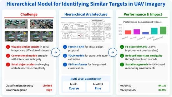
Conceptual diagram of the proposed two-phase hierarchical classification approach. In Phase 1 (Training), specialized datasets are prepared from UAV imagery to train the cascade. In Phase 2 (Inference), an initial detection model identifies Regions of Interest (ROIs), which are then fed into the multi-level classifier. This classifier operates as a coarse-to-fine cascade, where each level uses a dedicated feature map model and a classification model to progressively refine the object’s identity.
Figure 1.
Conceptual diagram of the proposed two-phase hierarchical classification approach. In Phase 1 (Training), specialized datasets are prepared from UAV imagery to train the cascade. In Phase 2 (Inference), an initial detection model identifies Regions of Interest (ROIs), which are then fed into the multi-level classifier. This classifier operates as a coarse-to-fine cascade, where each level uses a dedicated feature map model and a classification model to progressively refine the object’s identity.
Figure 2.
Modular data processing at a single classification level. A detected ROI is processed by a feature map model (e.g., YOLO) to create a feature vector. This vector is then classified by a separate Classification Model (e.g., FT-Transformer). This dual-model design decouples feature extraction from classification for optimized performance.
Figure 3.
The structured training workflow for each classification level. First, a feature map model is trained on a labeled image dataset. This model then generates a new dataset of feature vectors, which is subsequently used to train a separate, specialized classification model, ensuring both components are optimally tuned.
Figure 4.
The end-to-end inference pipeline. An initial detection model (Faster R-CNN) identifies all potential ROIs. Each ROI is then sequentially processed through the multi-level cascade, where its classification is progressively refined from general to specific, resulting in a final, accurately labeled object.
Figure 5.
An example of the three-level classification hierarchy, which follows a coarse-to-fine decision-tree structure. Level 1 separates objects into “Human” or “Vehicle,” focusing on the maximum inter-class distance. Level 2 refines the most populous class, “Vehicle,” into “Truck” or “Other Vehicle.” Level 3 further classifies “Other Vehicle” into “Van,” “Bus,” or “Other,” achieving granular identification.
Figure 6.
The specific deep learning models used in the three-level architecture. A Faster R-CNN model performs initial detection. Specialized YOLO models (YOLOv11m and YOLOv11s) then serve as feature extractors for subsequent levels. Finally, dedicated FT-Transformer models perform the classification at each stage, ensuring high accuracy.
Figure 7.
Visualization of feature vector separation using PCA for the optimal merging strategy at each classification level. (a) At the first level (Person vs. Vehicle), the concatenation of the last and penultimate layer vectors provides clear separation. (b) At the second level (Truck vs. Other Vehicle), combining the final layer with contour features is most effective. (c) At the third level (Van vs. Bus vs. Other Vehicle), the same strategy as the second level yields the best class distinction.
Figure 8.
Qualitative classification results illustrating the multi-level refinement process. (a) At Level 1, the model performs a general classification, identifying a “Person” (blue) and “Vehicles” (pink). (b) At Level 2, the classification is refined to identify a “Truck” (violet). (c) At Level 3, the model achieves fine-grained identification of a “Van” (orange).
Figure 9.
Confusion matrices for each classification level. Top row (a–c) shows the performance of the baseline feature extraction models using their standard classification heads. Bottom row (d–f) shows the improved performance of our proposed FT-Transformer classifiers, which use the feature vectors from the corresponding models.
Figure 10.
ROC curves for each classification level. The high AUC values for each level (1-layer: 0.95, 2-layer: 0.93, 3-layer: 0.96) demonstrate the excellent diagnostic ability and discriminative power of the models at each stage.
Figure 10.
ROC curves for each classification level. The high AUC values for each level (1-layer: 0.95, 2-layer: 0.93, 3-layer: 0.96) demonstrate the excellent diagnostic ability and discriminative power of the models at each stage.
Table 1.
Quantitative comparison of inter-class distances (unitless values in the PCA-reduced feature space) for various feature vector configurations across the three classification levels. The optimal distance for each level, indicating the best feature separation, is highlighted in bold.
Table 1.
Quantitative comparison of inter-class distances (unitless values in the PCA-reduced feature space) for various feature vector configurations across the three classification levels. The optimal distance for each level, indicating the best feature separation, is highlighted in bold.
| Vector | Inter-Class Distances |
|---|
| Level 1 | Level 2 | Level 3 |
|---|
| 3.90 | 1.80 | 1.58 |
| 4.20 | 1.74 | 1.64 |
| 3.0 | 2.38 | 1.84 |
| 3.67 | 2.01 | 1.78 |
Table 2.
Detailed performance metrics (in %) for each classification level for train and test subsets (SS). The results for both training and test sets demonstrate consistently high and stable performance, with low standard deviation (SD) calculated across three independent experimental runs.
Table 2.
Detailed performance metrics (in %) for each classification level for train and test subsets (SS). The results for both training and test sets demonstrate consistently high and stable performance, with low standard deviation (SD) calculated across three independent experimental runs.
| Level | SS | Precision | Recall | -Score |
|---|
| 1 | 2 | 3 | Avg | SD | 1 | 2 | 3 | Avg | SD | 1 | 2 | 3 | Avg | SD |
|---|
| 1 | Train | 95.2 | 95.5 | 95.8 | 95.5 | 0.3 | 94.6 | 94.8 | 94.1 | 94.5 | 0.4 | 94.4 | 94.7 | 94.2 | 94.4 | 0.3 |
| Test | 93.5 | 94.1 | 94.5 | 94.0 | 0.5 | 94.8 | 93.3 | 93.5 | 93.8 | 1.0 | 93.2 | 93.5 | 93.9 | 93.5 | 0.4 |
| 2 | Train | 93.7 | 93.2 | 94.0 | 93.6 | 0.4 | 95.8 | 95.7 | 96.9 | 96.1 | 0.8 | 95.9 | 95.1 | 96.3 | 95.7 | 0.6 |
| Test | 93.1 | 92.8 | 92.1 | 92.7 | 0.6 | 95.2 | 95.4 | 93.9 | 94.8 | 0.9 | 94.5 | 94.4 | 93.7 | 94.2 | 0.5 |
| 3 | Train | 95.9 | 94.8 | 95.3 | 95.3 | 0.6 | 97.1 | 97.3 | 96.4 | 96.9 | 0.5 | 95.9 | 96.1 | 95.0 | 95.7 | 0.7 |
| Test | 94.8 | 94.1 | 94.7 | 94.5 | 0.4 | 96.5 | 96.2 | 95.0 | 95.9 | 0.9 | 93.1 | 93.9 | 94.9 | 93.9 | 1.0 |
Table 3.
mAP scores (in %) for the complete cascaded system, evaluating performance on both training and test sets across different IoU thresholds. The results highlight the model’s high accuracy in both classification (mAP@.50) and precise object localization (mAP@.50:.95).
Table 3.
mAP scores (in %) for the complete cascaded system, evaluating performance on both training and test sets across different IoU thresholds. The results highlight the model’s high accuracy in both classification (mAP@.50) and precise object localization (mAP@.50:.95).
| Subset | mAP@.50 | mAP@.50:.95 |
|---|
| 1 | 2 | 3 | Avg | SD | 1 | 2 | 3 | Avg | SD |
|---|
| Train | 95.1 | 95.2 | 94.5 | 94.9 | 0.4 | 84.1 | 86.8 | 85.4 | 85.4 | 1.4 |
| Test | 94.5 | 94.1 | 93.7 | 94.1 | 0.4 | 83.8 | 82.3 | 83.1 | 83.0 | 0.8 |
Table 4.
Generalization performance on the unseen COCO dataset (in %). Precision, Recall, and -score are reported per level, while mAP scores reflect the aggregate performance of the complete three-level cascade.
Table 4.
Generalization performance on the unseen COCO dataset (in %). Precision, Recall, and -score are reported per level, while mAP scores reflect the aggregate performance of the complete three-level cascade.
| Level | Precision | Recall | -Score | mAP@.50 | mAP@.50:.95 |
|---|
| 1 | 93.2 | 93.1 | 94.0 | – | – |
| 2 | 92.8 | 94.7 | 94.2 | – | – |
| 3 | 94.2 | 94.9 | 93.7 | 93.5 | 80.1 |
Table 5.
Generalization performance on the unseen UAV123 dataset (in %). Precision, Recall, and -score are reported per level, while mAP scores reflect the aggregate performance of the complete three-level cascade.
Table 5.
Generalization performance on the unseen UAV123 dataset (in %). Precision, Recall, and -score are reported per level, while mAP scores reflect the aggregate performance of the complete three-level cascade.
| Level | Precision | Recall | -Score | mAP@.50 | mAP@.50:.95 |
|---|
| 1 | 92.8 | 92.4 | 92.9 | – | – |
| 2 | 92.1 | 92.9 | 93.1 | – | – |
| 3 | 93.1 | 93.5 | 93.0 | 92.1 | 78.4 |
Table 6.
Comparison (in %) of the proposed feature vector construction method with the standard model. The proposed method, using a transformer-based classifier, yields significantly better results across all metrics.
Table 6.
Comparison (in %) of the proposed feature vector construction method with the standard model. The proposed method, using a transformer-based classifier, yields significantly better results across all metrics.
| Method | Precision | Recall | -Score |
|---|
| Proposed feature vector construction method | 93.73 | 94.83 | 93.87 |
| Standard fully connected layer model for classification | 90.73 | 92.40 | 92.46 |
Table 7.
Comparison (in %) of the proposed method with existing approaches on the VisDrone2019 dataset. The proposed multi-level classification approach demonstrates competitive performance against other state-of-the-art methods. Higher values are shown in bold.
Table 7.
Comparison (in %) of the proposed method with existing approaches on the VisDrone2019 dataset. The proposed multi-level classification approach demonstrates competitive performance against other state-of-the-art methods. Higher values are shown in bold.
| Method | Precision | Recall | -Score |
|---|
| Yan et al. [9] | 94.5 | 94.0 | 93.2 |
| Zhang et al. [10] | 91.4 | 91.0 | 91.4 |
| Fine-tuned YOLOv8m [36] | 92.4 | 93.8 | 94.1 |
| Our approach | 93.7 | 94.8 | 93.9 |
Table 8.
Comparative performance analysis (in %) on the UAV123 dataset (test split, averaged over three runs). Baselines were re-trained with our protocol for a fair comparison. Methods are linked to
Section 1.2 via citations. Higher values are shown in
bold.
Table 8.
Comparative performance analysis (in %) on the UAV123 dataset (test split, averaged over three runs). Baselines were re-trained with our protocol for a fair comparison. Methods are linked to
Section 1.2 via citations. Higher values are shown in
bold.
| Method | -Score | mAP@.50 | mAP@.50:.95 |
|---|
| Faster R-CNN (baseline) | 88.7 | 86.9 | 69.2 |
| Fine-tuned YOLOv8m [36] | 91.7 | 90.2 | 75.1 |
| MCA-YOLOv7 [14] | 91.0 | 89.8 | 73.5 |
| DV-DETR (RT-DETR variant) [16] | 90.9 | 89.4 | 74.0 |
| Our approach | 93.0 | 92.1 | 78.4 |


