4.1. Algorithm Specification
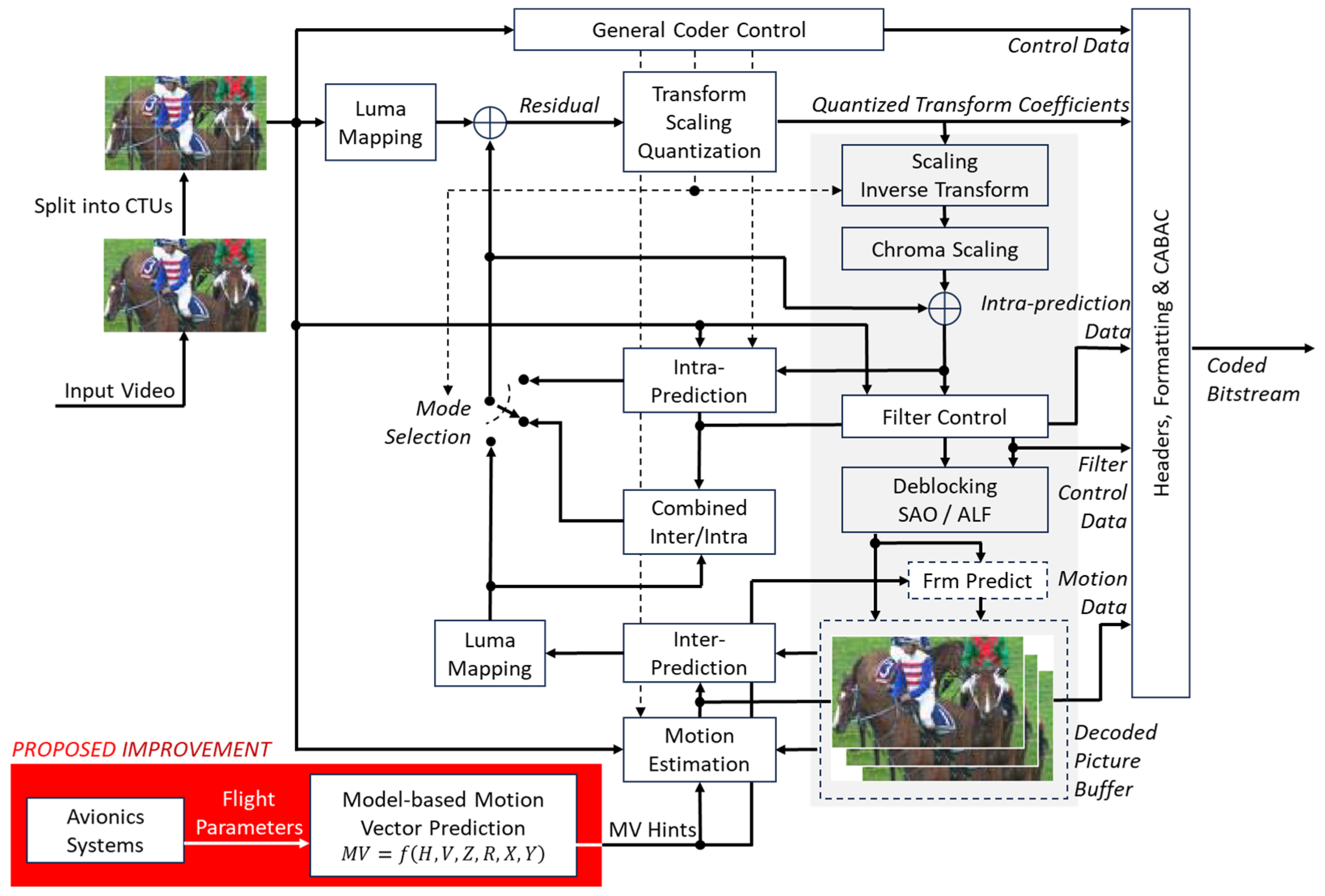
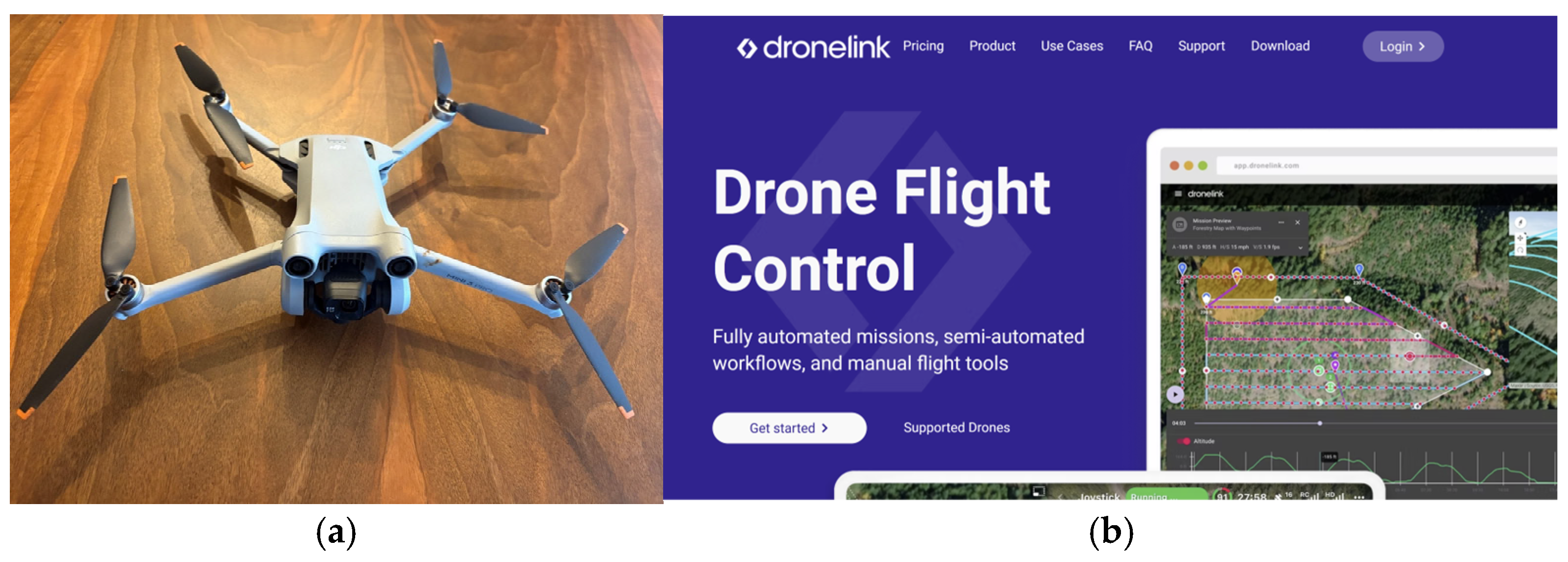
To develop the intended motion model, a drone equipped with a high-resolution camera and auto-pilot capabilities was selected. The terrain over which the drone would fly was marked with easily distinguishable visual markers. Three basic motion types were defined, translational, rotational, and elevational (ascending/descending). The final complex motion was defined as the superposition of these three basic motion types.
For each basic motion type, multiple sets of flight parameters were selected. Corresponding flight plans were generated within the auto-pilot application and validated using its built-in simulation environment. The drone was then autonomously flown over the marked terrain multiple times, following these predefined flight plans. During each flight, video footage was recorded using the onboard camera.
Each recorded video was processed using a custom application developed with the OpenCV library. The positions of the markers in each video frame were detected, and their motion vectors were computed for temporal intervals of 5 and 25 frames. This formed the dataset used to define the motion model.
Temporal intervals of 5 and 25 frames were specifically selected since they are widely used for real-world streaming GOP sequences. For 4K or 8K content at 50 or 100 fps, a GOP size of 25 or multiples of 25 frames are utilized: GOP structure starts with an I-frame and P-frames are utilized at regular intervals, say at every two to four B-frames between them. This is a closed GOP structure and is generally used for streaming applications. In such a GOP structure, the coding sequence is generally organized as I, B, B, B, P, B, B, B, P…, and the number of B-coded frames in between two I- or P-coded frames generally varies from two to four. TD = 5 is selected to easily detect MV between two I- or P- frames, and smaller temporal distances can be found by interpolation.
For every basic motion type and associated set of flight parameters, a polynomial surface fitting was performed for the motion vector components MVx and MVy, relative to normalized coordinates within the video frame. Subsequently, for each coefficient obtained from this fitting process, a secondary polynomial surface fit was carried out with respect to the corresponding flight parameters. As a result, two mathematical motion models (corresponding to 5- and 25-frame intervals) were derived for each of the three basic motion types.
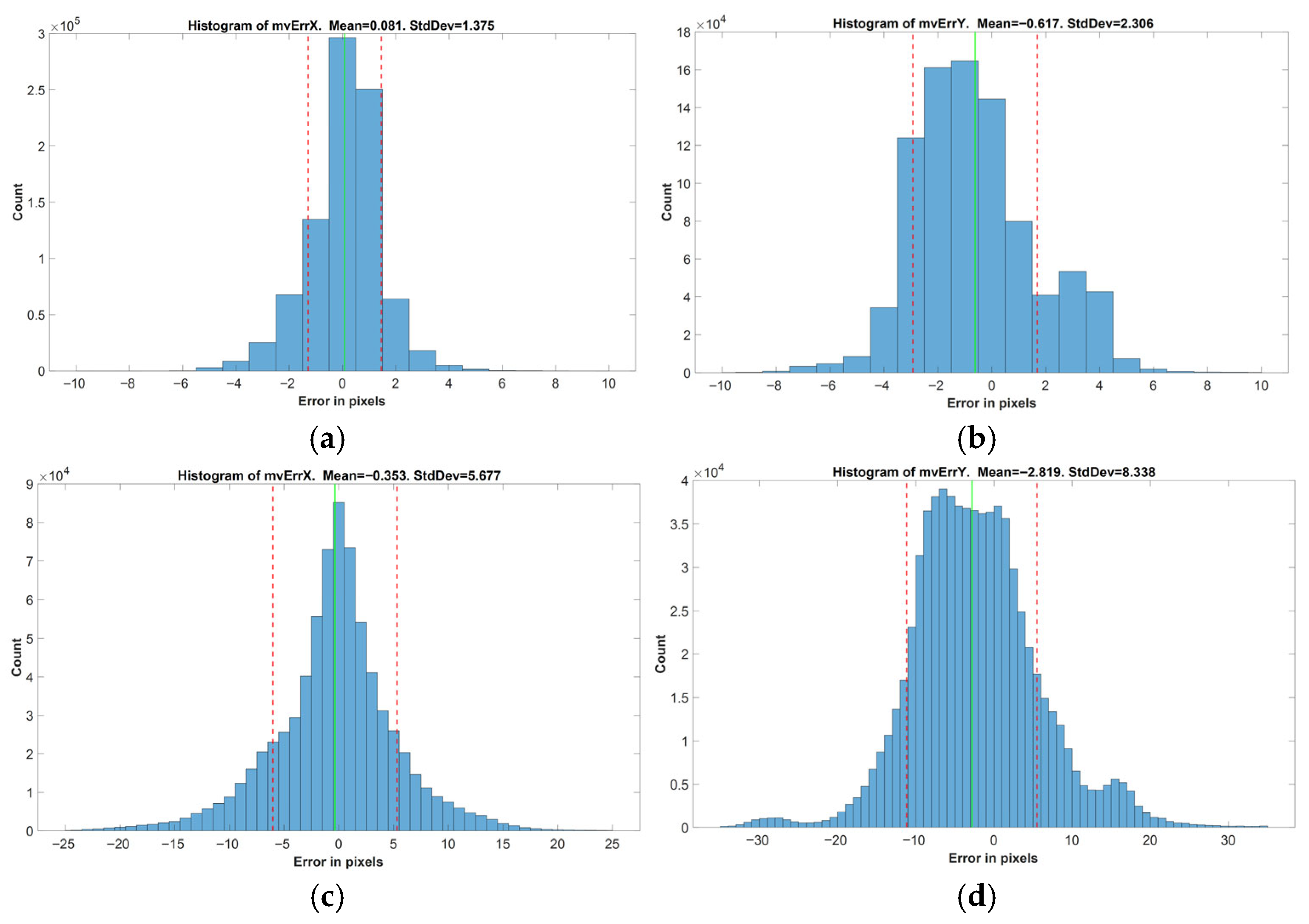
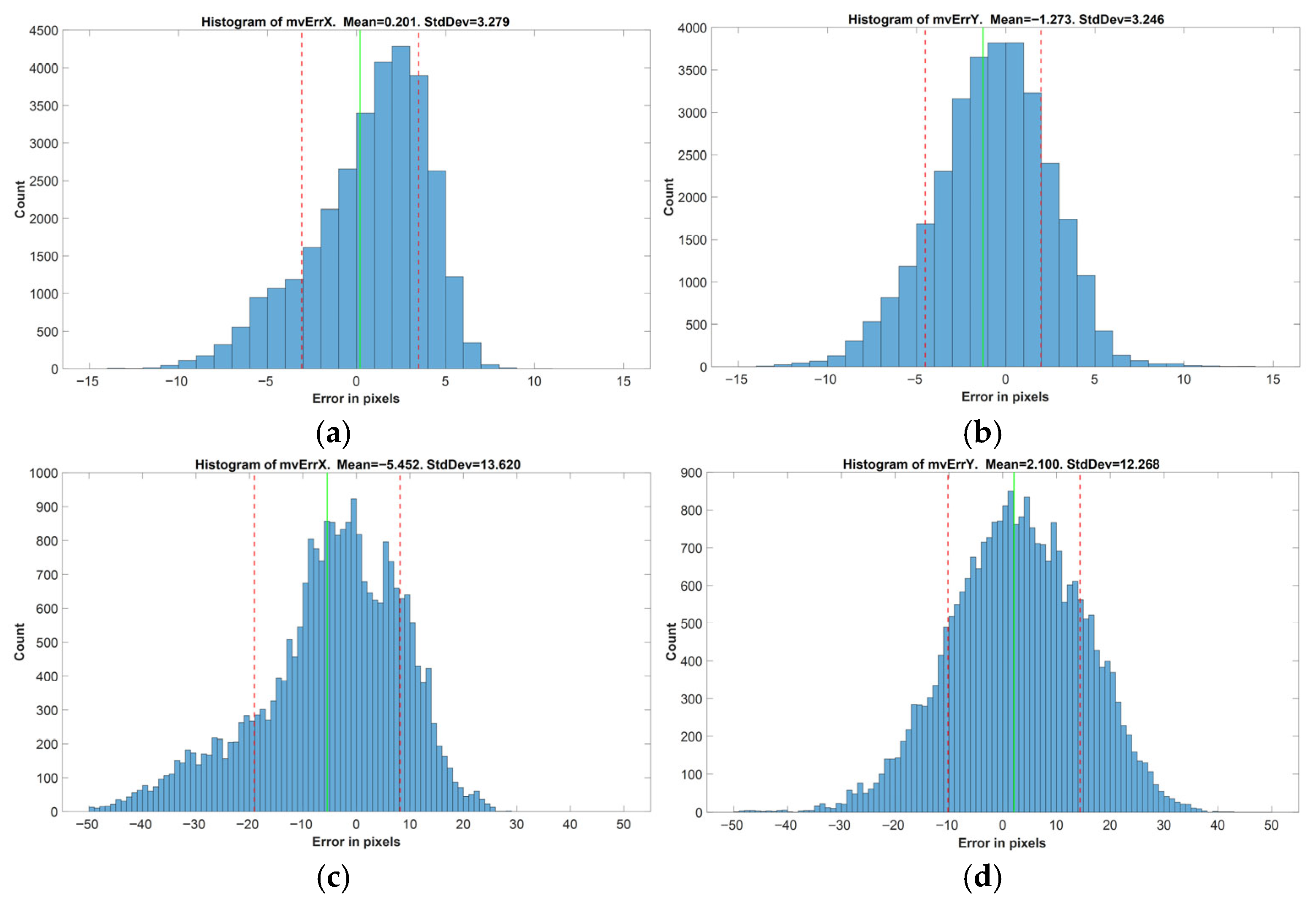
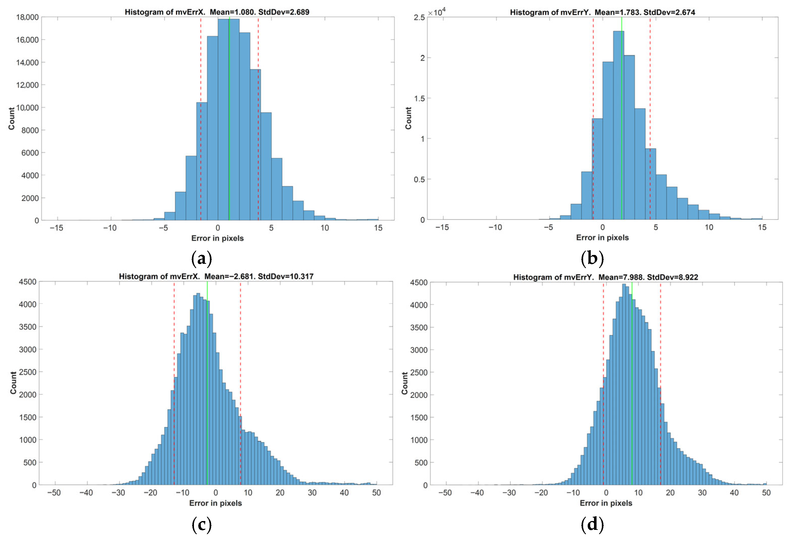
To evaluate the accuracy of the basic motion models, motion vectors for each marker in every video frame were computed using the constructed models and compared against the actual vectors from the dataset. The resulting differences were considered as the errors introduced by the models. Error distributions for MVx and MVy components were analyzed independently, and their mean and standard deviation values were computed. This evaluation procedure was repeated for all basic motion types across both temporal intervals.
Upon completion of the basic motion model construction and corresponding error analysis, a final complex motion model was established as the vectorial summation (superposition) of the three basic motion models.
To assess the accuracy of the complex motion model, additional flight plans were created involving combined motion types: ramp (translation + elevation), orbit (translation + rotation), and helix (translation + rotation + elevation). The drone was flown over the same marked terrain under auto-pilot control using these plans, and additional test videos were obtained.
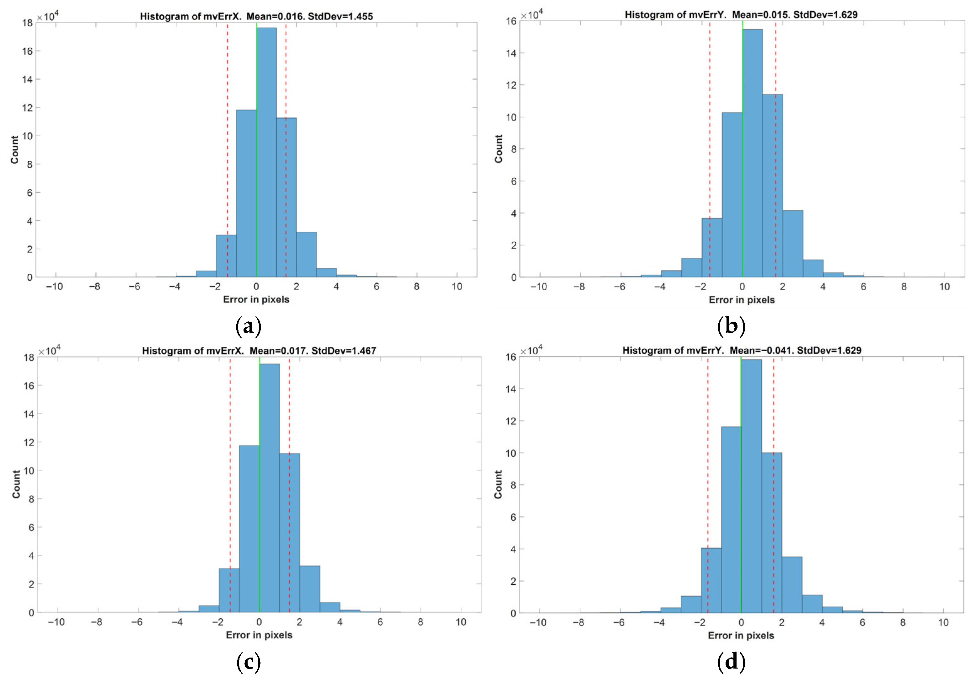
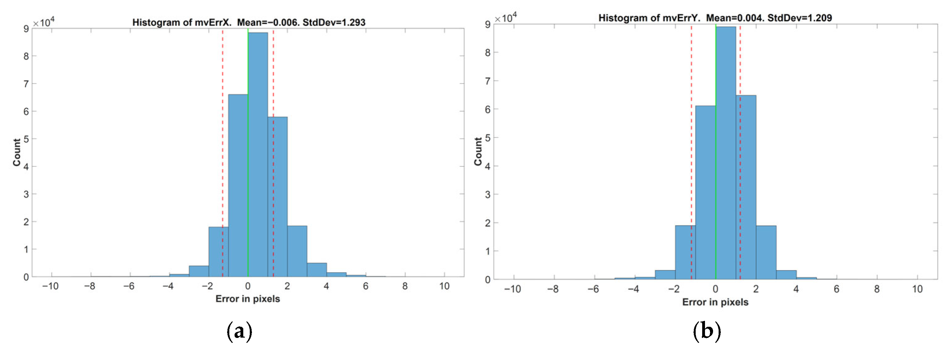
For each frame in the test videos, motion vectors of the markers were calculated using both the OpenCV-based application and previously developed complex motion model. The discrepancies between these vectors were considered as errors introduced by the complex model. Histograms of the error in MVx and MVy components were generated, and their statistical properties (mean and standard deviation) were evaluated for both 5- and 25-frame temporal intervals.
To conclude, a polynomial surface fit-based mathematical motion model was developed for estimating motion vectors from drone-captured video by using the flight data of the drone.
4.4. OpenCV Processing of Recorded Video and Use of MATLAB Tools
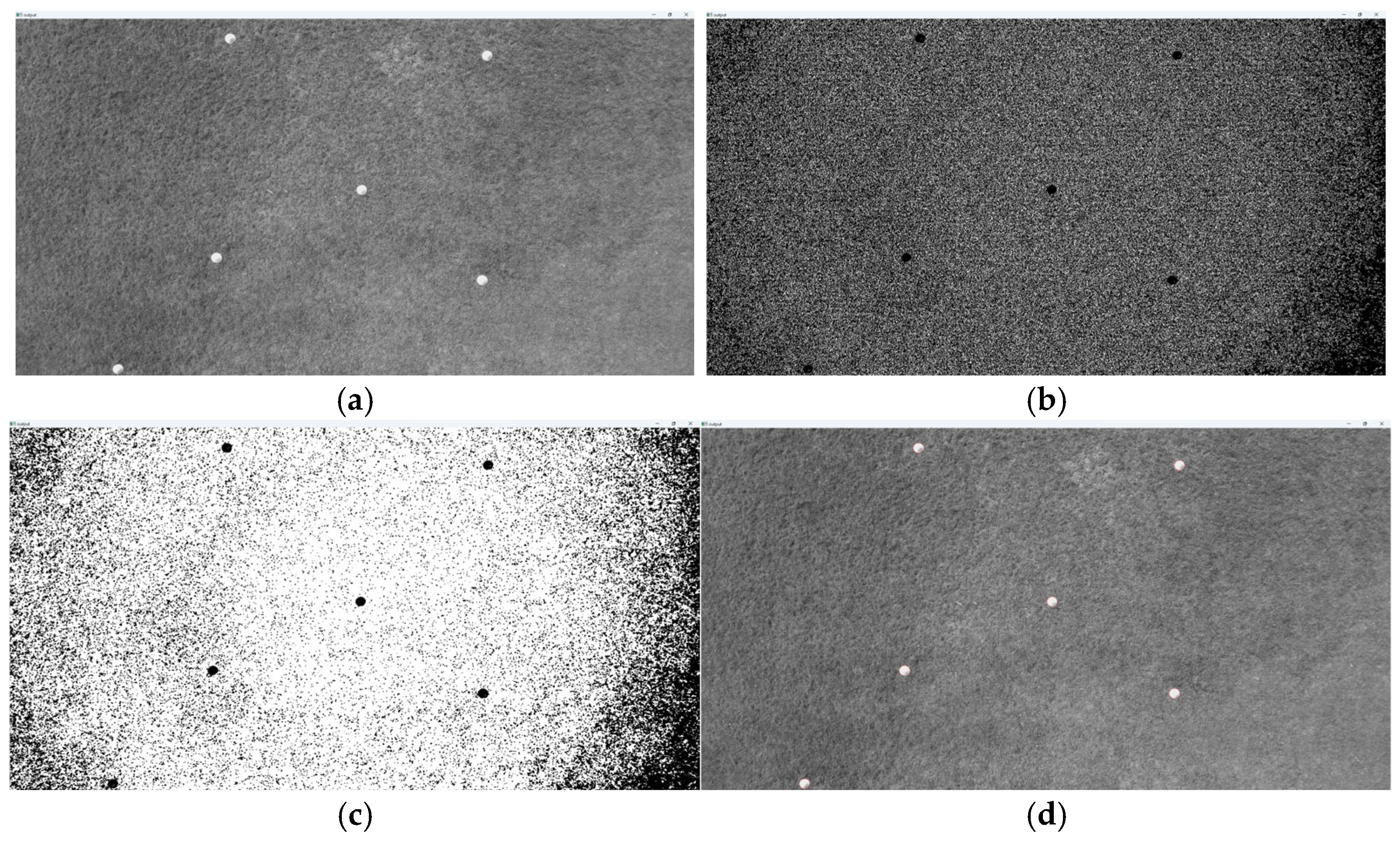
To process the recorded videos and quantitatively detect the positions of the markers on video frames, an application using OpenCV version 4.10 is developed. This application processes each and every frame of the input video, detects markers on each frame, draws the trajectories, and calculates the motion vectors of each marker for the temporal distances of 5 and 25 frames.
In order to detect the markers on the video frames, Canny edge detection, dilation, erosion, and blob detection algorithms were used. Since the marker sizes in the captured video tend to get smaller as the flight level the video is recorded at increases, the detection parameters are varied accordingly.
During the processing of video frames with OpenCV tools, only the luma component is used, and the chroma is discarded.
Figure 4 illustrates the processing stages of a sample frame captured at flight level H = 10 m.
During the processing of the captured videos, the initial seconds that contain the acceleration of the drone to the requested flight parameters and the final seconds that contain the deceleration to a stationary state are discarded. Only the steady state parts of the video with the requested flight parameters are processed. A total of 154 video files with 91 GB size are recorded and processed that way.
Afterwards, for the motion vectors of the markers extracted from the recorded video files, two-dimensional polynomial surface fitting is implemented by using the MATLAB R2024b environment. The fit() function with poly11, poly22 or poly33 settings are used for this purpose.
Finally, during the performance evaluation of the constructed motion models, the histogram of the error values is drawn. For this purpose, histogram(), mean() and std() functions are used, and the graphics produced are included in this paper.
4.5. Modeling of Basic Translational Motion
In order to independently model the basic translational motion of the drone, 90 video files are captured and processed at all combinations of = {5, 10, 15, 20, 25, 30, 40} (flight level, m) and = {1, 2, 3, 4, 5, 6} (translational velocity, m/s).
As illustrated in
Figure 5, the flight plan over the marked terrain is prepared and verified. The drone repeatedly flies over the marked terrain at different flight levels with a fixed translational velocity. The flight plan is repeated for all available translational velocity settings. During the straight forward paths, the video coming from the downward-facing camera onboard the drone is captured.
After all the flights are complete, a set of 90 video files is processed using the analysis software written by using OpenCV 4.10, markers are detected, marker trajectories are visualized, and the motion vectors corresponding to the markers are calculated.
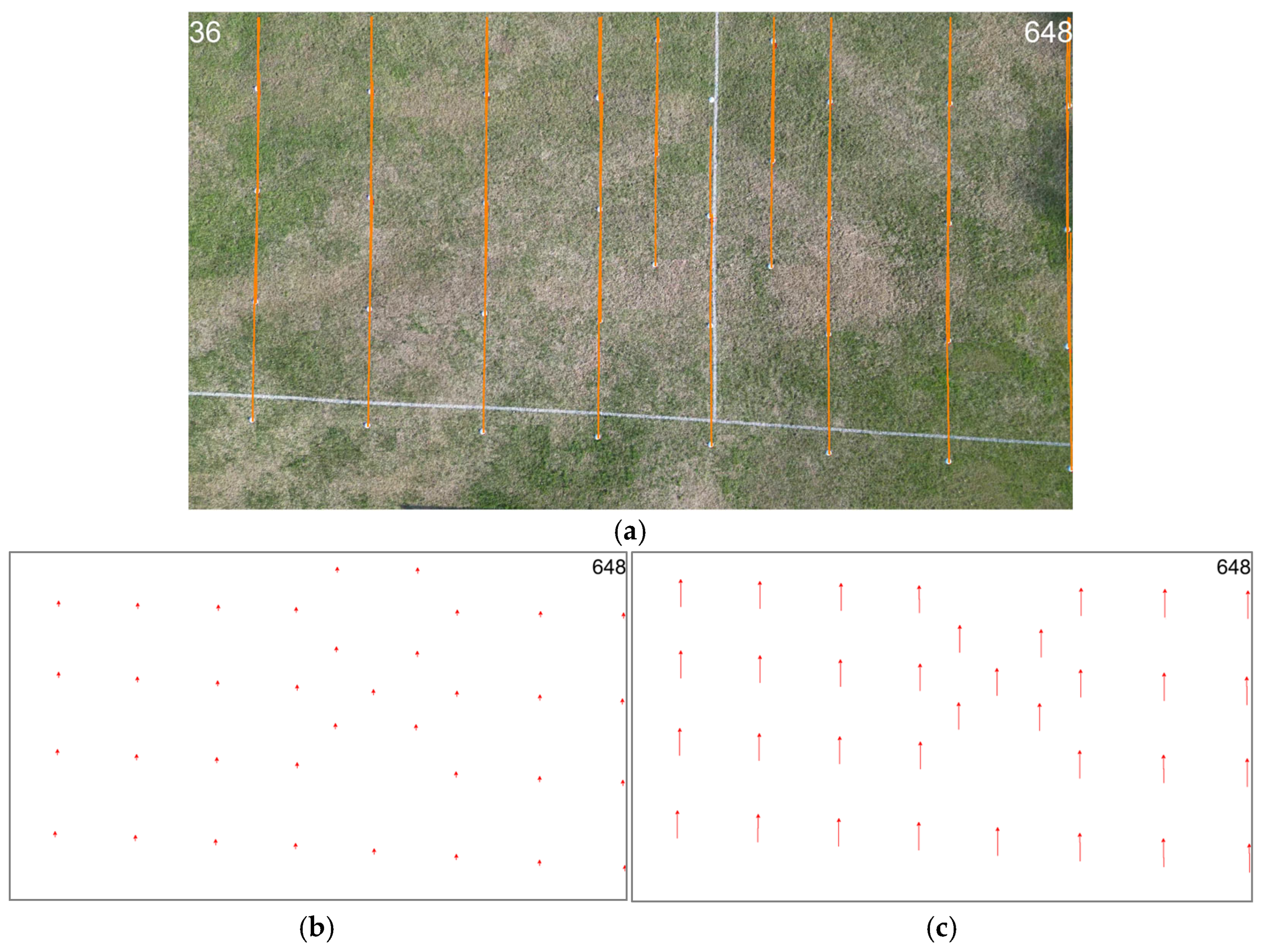
Figure 6a illustrates an example for how the marker trajectories (orange lines) are visualized for the basic translational motion type. The video used as an example here is shot at flight level
= 25 m with a translational velocity of
= 3 m/s. Since the drone is going straight forward, markers in the video are translating downwards.
By using the positions of the markers on each frame, motion vectors corresponding to every marker at every frame are calculated for two different temporal distances.
Figure 6b illustrates the motion vectors for frame #648 of the example video file for a temporal distance of TD = 5 frames, whereas
Figure 6c illustrates the motion vectors for TD = 25.
For each and every video frame of the video file, detected motion vectors for a fixed temporal distance value are dumped as a CSV file in the format illustrated in
Table 1.
(Xa,Ya) are the absolute and (Xn,Yn) are the normalized coordinates of the motion vectors. In reality, these correspond to the marker location on the video frame. Normalized coordinates are derived by dividing the absolute coordinates by the resolution of the video frame and vary in the range [0, 1). (MVx,MVy) denotes the X and Y components of the calculated motion vector in pixels. H denotes the flight level.
This file is then analyzed by MATLAB R2024b tools, and two-dimensional surface fits are performed for the motion vector components. To illustrate the dataset used to model
MVx, corresponding data in
Table 1 is marked with a blue background. Both poly11 and poly22 type fits are performed. As a result, for this flight level and translational speed setting, a polynomial model for the motion vectors for that temporal distance value is constructed as in the following equation:
are the normalized coordinates of the location of the object on the video frame in the range [0, 1), and is the 2D motion vector for that temporal distance value. The polynomial coefficients are also 2D vectors.
Figure 7 illustrates the surface fits for the X- and Y-components of the motion vectors for the example video file for a temporal distance of 5 frames. In this illustration, OpenCV detected motion vector components are illustrated as the blue-white grid, poly11 fit is illustrated as the planar yellow-black surface, and the poly22 fit is illustrated as the curved green surface.
Table 2 illustrates the polynomial fit parameters for each MV component.
This procedure is repeated for every translational motion test video captured at different flight levels () and translational velocities () for the same temporal distance setting. That way, a coefficient set for poly11 and poly22 fits are obtained for the translational motion vectors with respect to the normalized object coordinates on the video frame. Due to the fact that non-linear behavior is introduced by poly22 fits, poly11 fits are selected.
As illustrated in
Table 3, poly11 fit coefficients for different flight parameters are grouped together and dumped to a new CSV file. In other words, polynomial surface fit coefficients calculated for all specific flight parameters are accumulated in this new file. The first two columns are the flight parameters, following three columns are the poly11 surface fit coefficients of the X-component, and the final three columns are the poly11 surface fit coefficients of the Y-component of the motion vectors.
To illustrate this process, the flight parameters shown by orange cells, poly11 fit coefficients of
MVx shown by blue cells, and poly11 fit coefficients of
MVy shown by green cells in
Table 2 are copied to the corresponding locations in the CSV file, as shown in
Table 3.
Our objective at this stage is to construct secondary models for poly11 surface fit parameters
,
,
,
,
, and
in
Table 3 in terms of the flight parameters
and
. For each of the six poly11 surface fit parameters listed above, poly11-, poly22-, and poly33-based secondary surface fits with respect to the flight parameters of
and
are performed and polynomial models as in (5) are defined.
To explain this process further, by using the data illustrated in
Table 4, the surface fits for the
and
coefficients illustrated in
Figure 8 are obtained. In
Table 4, grey cells illustrate the data used to derive the model for
and the italic cells illustrate the data used to derive the model for
fit parameter.
In
Figure 8, X and Y coordinates are the flight parameters for the translational motion, and the Z coordinate is the
coefficient for the X- and Y-components of the motion vector. Coefficient data derived at the preceding step is illustrated by using the blue-white grid structure, and the poly33 fit is illustrated by using the dark blue curved surface. This procedure is repeated for the
,
,
,
,
, and
fit coefficients listed in
Table 3, and poly33 fit is preferred. The motion model obtained for the translational motion is in the form of (3) and (4)
where each coefficient is modeled as a general third order polynomial function of flight parameters
(flight level) and
(translational velocity) in the form of (5).
For every parameter, there is a different set of [, , , , , , , , , ] third order surface fit coefficients. Six different parameters, each with a ten-element coefficient set, give us a sixty-parameter motion model for the temporal distance of TD = 5 frames.
This procedure is run for two different temporal distances: 5 and 25 frames. Two different basic translational motion models for the motion vectors are constructed, as explained in the preceding paragraphs. The coefficient set for TD = 5 is listed in
Table 5, and the coefficient set for TD = 25 is listed in
Table 6.
4.6. Modeling of Basic Rotational Motion
In order to independently model the basic rotational motion of the drone, 40 video files are captured and processed at all combinations of = {5, 10, 15, 20, 25, 30, 40} (flight level, m) and = {20, 30, 40, 50, 60} (rotational rate, deg/s).
As illustrated in
Figure 9, the flight plan over the marked terrain is prepared and verified. The drone repeatedly flies over the marked terrain at different flight levels, with a fixed rotational rate along its
Z-axis.
It is elevated to the desired flight level, settles there, starts rotating around in a clockwise direction at the desired rate, stops when a predetermined time elapses, elevates to the next flight level and rotates again, and so forth. During the rotation motion along its Z-axis, the flight level is kept constant, and the video coming from the downward-facing camera onboard the drone is captured.
After all the flights are complete, a set of 40 video files is processed using the analysis software written by using OpenCV, acceleration and deceleration transients at the beginning and end of the video files are discarded, markers are detected at the steady state rotation phase, marker trajectories are visualized, and the motion vectors corresponding to the markers are calculated.
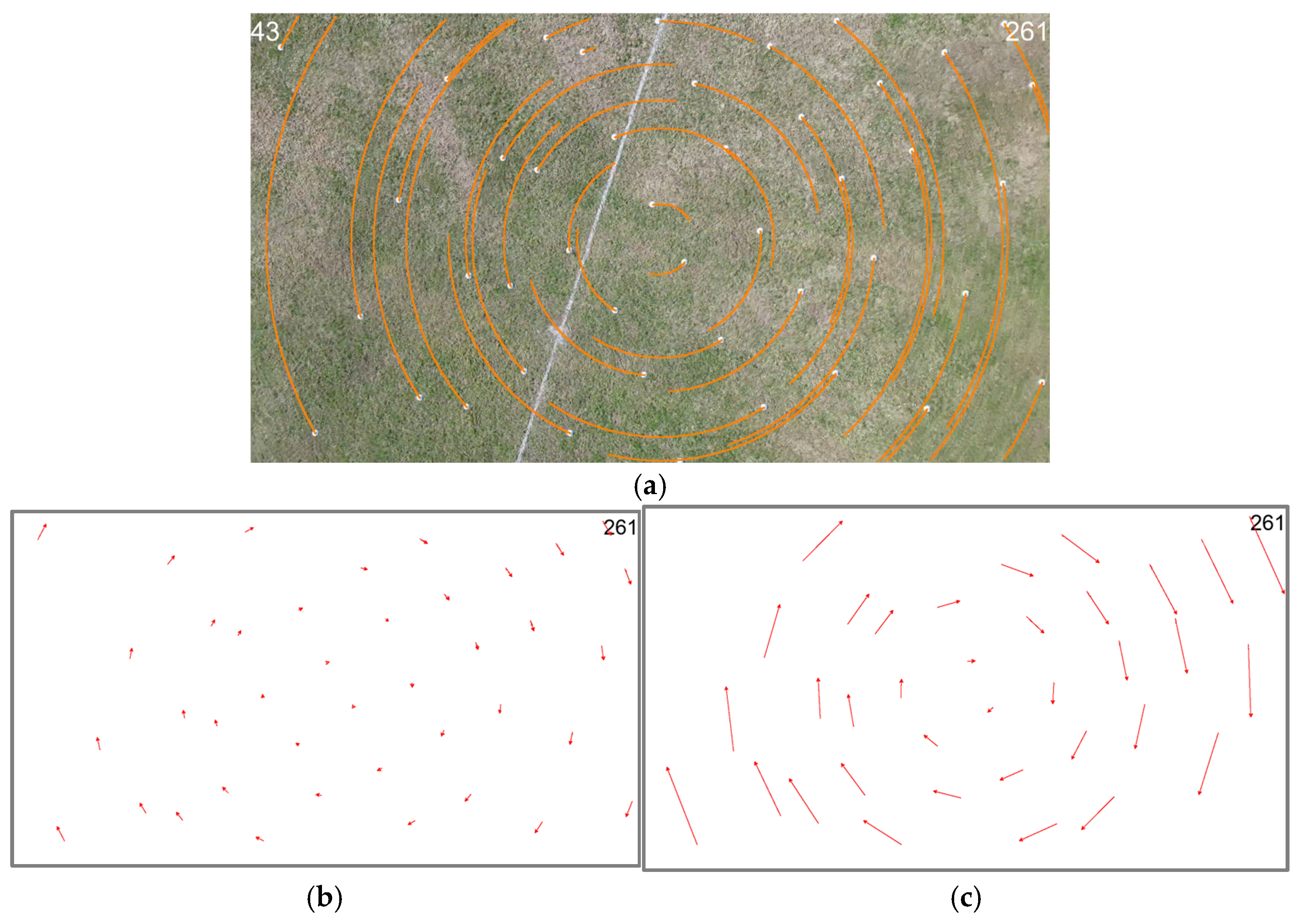
Figure 10a illustrates an example of how the marker trajectories are visualized for the basic rotational motion type. The video used as an example here is shot at flight level
= 20 m and a rotational rate of
= 30 degrees/s. Since the drone is rotating along its
Z-axis, the markers in the video are in a circular motion. The orange lines are the trajectories of the markers.
By using the positions of the markers on each frame, motion vectors corresponding to every marker at every frame are calculated for two different temporal distances.
Figure 10b illustrates the motion vectors for the frame #261 of the example video file for the temporal distance of TD = 5 frames, whereas
Figure 10c illustrates them for TD = 25 frames.
For each and every video frame of the video file, detected motion vectors for a fixed temporal distance value are dumped as a CSV file in the format illustrated in
Table 7.
(Xa,Ya) are the absolute and (Xn,Yn) are the normalized coordinates of the motion vector and they vary in the range [0,1). (MVx,MVy) denotes the X and Y components of the calculated motion vector in pixels. H denotes the flight level. It is not used for the analysis and modeling of the translational and rotational motion, only for the analysis of elevational (ascending/descending) motion.
This file is then analyzed by MATLAB tools, and two-dimensional surface fits are performed for the motion vector components. To illustrate the dataset used to model
MVx, the corresponding data in
Table 7 is marked with a blue background. Both poly11 and poly22 type fits are performed. As a result, for this flight level and rotation rate setting, a polynomial model for the motion vectors for that temporal distance value is constructed as in (2).
Here, are the normalized coordinates of the location of the object on the video frame in the range [0, 1), and is the 2D motion vector for that temporal distance value. The polynomial coefficients are also 2D vectors.
Figure 11 illustrates the surface fit for the X- and Y-component of the motion vectors for the example video file for a temporal distance of 5 frames. In this illustration, OpenCV-detected motion vector component values are illustrated as the blue-white grid, poly11 fit is illustrated as the planar yellow-black surface, and the poly22 fit is illustrated as the curved green surface.
Table 8 illustrates the polynomial fit parameters for each MV component.
As can be observed from
Figure 11, the fits are mostly planar, not curved. Also, it can be observed from
Table 8 that the fit coefficients [
] of poly11 and poly22 type fits are nearly identical, and the other coefficients of poly22 fit are very small compared to them. This shows us that the difference between the poly11 and poly22 fits will be incremental.
This procedure is repeated for every rotational motion test video captured at different flight levels () and rotational rates () for the same temporal distance setting. That way, a coefficient set for poly11 and poly22 fits are obtained for the rotational motion vectors with respect to the normalized object coordinates on the video frame.
As illustrated in
Table 9, poly11 fit coefficients for different flight parameters are grouped together and dumped to a new CSV file. The first two columns are the flight parameters, the following three columns are the poly11 surface fit coefficients of the X-component, and the final three columns are the poly11 surface fit coefficients of the Y-component of the motion vectors.
To illustrate this process, the flight parameters shown by orange cells, the poly11 surface fit coefficients of the
MVx component shown by blue cells, and the poly11 surface fit coefficients of the
MVy component shown by the green cells in
Table 8 are copied to the corresponding locations in the new CSV file, as illustrated in
Table 9.
Additionally, as illustrated in
Table 10, poly22 fit coefficients for different flight parameters are also grouped together and dumped to another CSV file. The first two columns are the flight parameters, the following six columns are the poly22 surface fit coefficients of the X-component, and the final six columns are the poly22 surface fit coefficients of the Y-component of the motion vectors.
To illustrate this process, the flight parameters shown by orange cells, the poly22 surface fit coefficients of the
MVx component shown by blue cells, and the poly22 surface fit coefficients of the
MVy component shown by the green cells in
Table 8 are copied to the corresponding locations in the new CSV file, as illustrated in
Table 10.
Our objective at this stage is to construct secondary models for six poly11 surface fit parameters
,
,
,
,
, and
—in
Table 9 and twelve poly22 surface fit parameters
,
,
,
,
,
,
,
,
,
,
, and
—in
Table 10 in terms of the flight parameters
and
. Therefore, for each and every one of those parameters, poly11, poly22, and poly33 surface fits with respect to the flight parameters of
and
are performed. This is again performed for the same temporal distance.
To explain this process further, the data marked with italic numbers in
Table 9 is used to construct the surface fits for the
coefficient of the poly11 fit model, and the data marked with italic numbers in
Table 10 is used to construct the surface fits for the
coefficient of the poly22 fit model. All coefficients are surface fit for both the poly11 fit and the poly22 fit model, and the performance of both models are compared.
Figure 12 illustrates the poly33 surface fit for the
and
coefficients of the poly22 fit model. Please note that the X and Y coordinates are the flight parameters for the rotational motion, and the Z coordinate is the
coefficient for the X- and Y-components of the motion vector. Coefficient data derived at the preceding step is illustrated by using the blue-white grid structure, and the poly33 fit is illustrated by using the dark blue curved surface. Note that the fitting surfaces are almost planar.
The motion model obtained for the basic rotational motion in the case of poly11 fit is in the following form:
whereas in the case of poly22 fit, it is in the following form:
where each coefficient is modeled as a general third order polynomial function of flight parameters
(flight level) and
(rotational rate) in the following form:
For every parameter, there is a different set of [, , , , , , , , , ] third order surface fit coefficients. For the poly11 fit-based motion model, there are 6 different parameters, each with a ten-element coefficient set, giving us a 60-parameter motion model, whereas for the poly22 fit-based motion model, there are twelve different parameters, each with a ten-element coefficient set, giving us a 120-parameter motion model.
The coefficients of poly11 and poly22 fits are so close that the difference between them is incremental. The success rates of both models are studied, and no meaningful difference between them is observed. For the temporal distance TD = 5 model, the poly11 fit-based rotational motion model is selected, whereas for temporal distance TD = 25 model, since the motion vectors are longer, the poly22 fit-based rotational motion model is selected, for higher precision.
This procedure is run for two different temporal distances, 5 and 25 frames, and two different basic rotational motion models for the motion vectors are constructed, as explained in the preceding paragraphs. The coefficient set for TD = 5 is listed in
Table 11, but the coefficient set for TD = 25 is omitted due to space concerns. Please note that, for every
coefficient, the first three fit parameters [
,
,
] are larger than the rest of the parameters, which gives flat surfaces.
4.7. Modeling of Basic Elevational (Ascending/Descending) Motion
In order to model the basic elevational motion, 10 video files are captured and processed for
= {−3, −2, −1, 1, 2, 3} (ascend/descend rate, m/s). As illustrated in
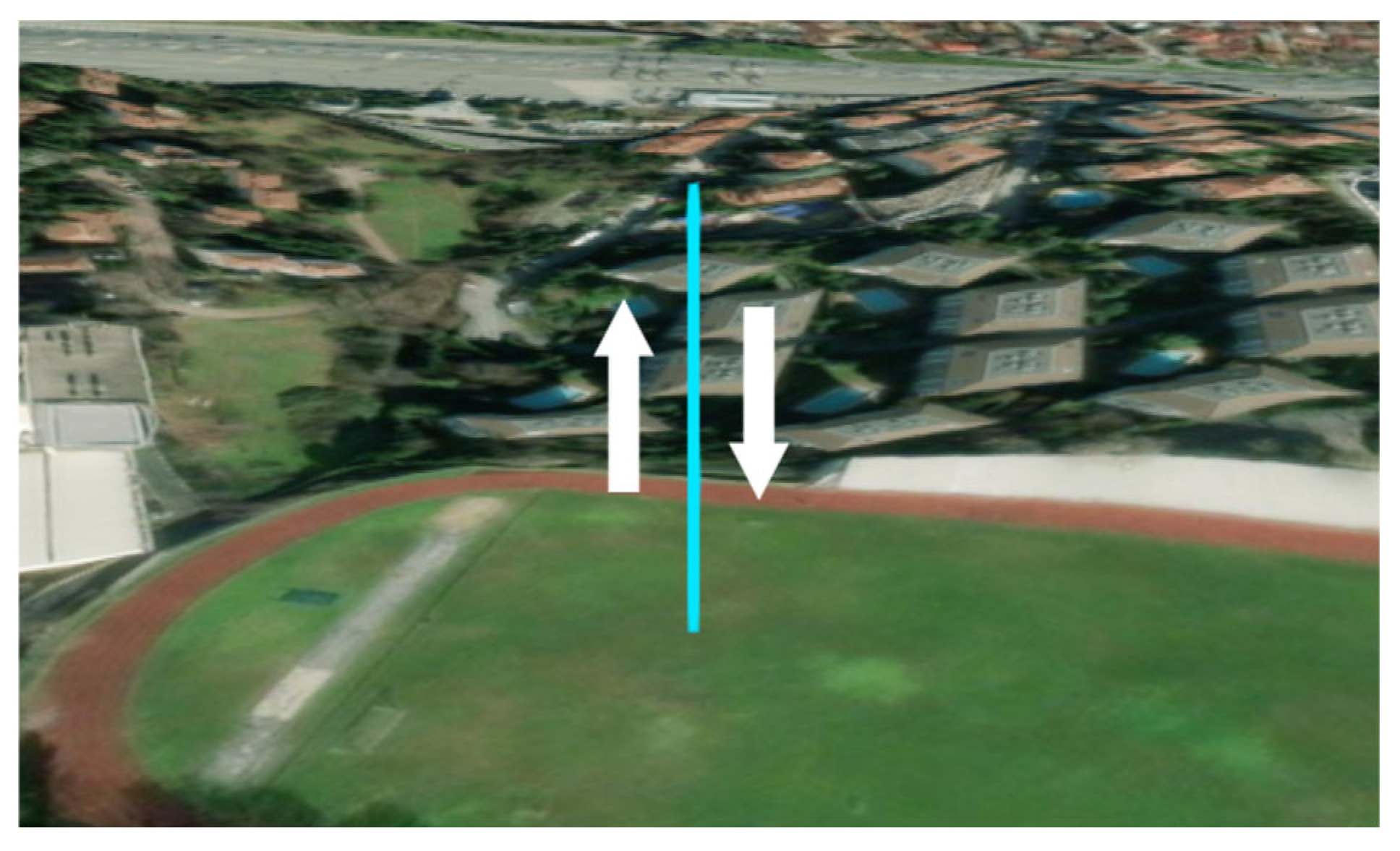
Figure 13, the flight plan over the marked terrain is prepared and verified in the simulator environment.
The drone starts at ground level, ascends to a 45 m flight level with a fixed elevational rate, settles there, starts descending with the same rate, and finally lands on the ground. During the elevational motion along its Z-axis, the video coming from the downward-facing camera is captured. This sequence is repeated for different elevational rates as stated.
After all the flights are complete, a set of 10 video files is processed using the analysis software written by using OpenCV, acceleration and deceleration transients at the beginning and end of the video files are clipped, markers are detected at the steady state ascending/descending phase, marker trajectories are visualized, and the motion vectors corresponding to the markers are calculated.
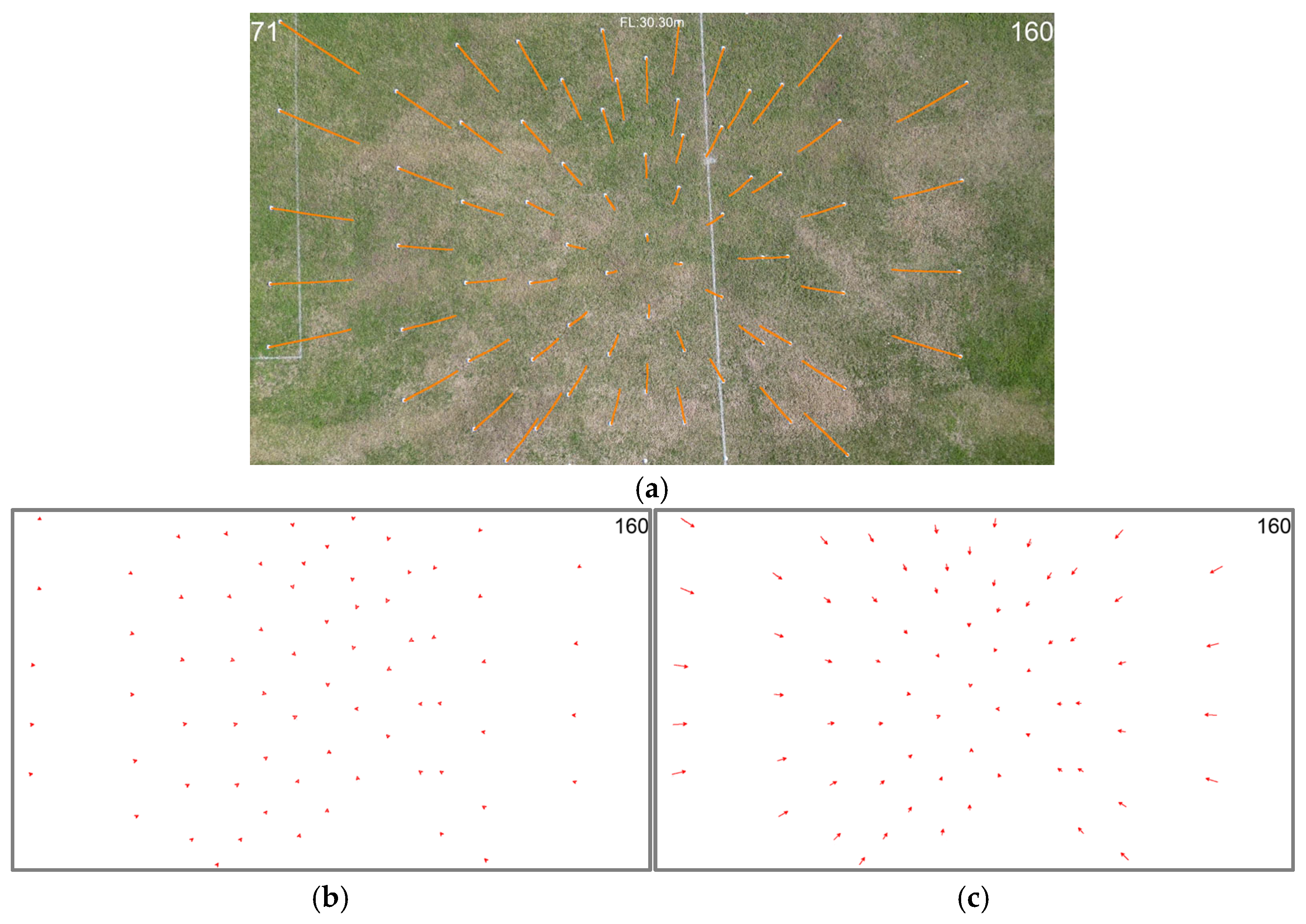
Figure 14a illustrates an example of how the marker trajectories are visualized for the elevational motion type. The video used as an example here is shot with an elevational rate of
= −3 m/s. The video frame in the figure corresponds to flight level
= 30 m. Since the drone is descending along its
Z-axis, the markers in the video are moving away from the center towards the periphery. The orange lines are the trajectories of the markers.
By using the positions of the markers on each frame, motion vectors corresponding to every marker at every frame are calculated for two different temporal distances.
Figure 14b illustrates the motion vectors for frame #159 of the example video file for the temporal distance TD = 5 frames, whereas
Figure 14c illustrates the motion vectors for the temporal distance TD = 25 frames. The flight level
= 30 m for those samples.
Exactly the same procedure applied for the modeling of the basic rotational motion is also applied for the basic elevational motion. The motion vectors for the markers on the video frames are extracted, and 2D surface fits with respect to the normalized object coordinates are applied.
At this stage, poly11 and poly22 fits are utilized. Afterwards, poly33 fits to those surface fit coefficients with respect to the flight parameters are carried out. For the temporal distance TD = 5 model, the poly11 fit-based elevational motion model is selected, whereas for temporal distance TD = 25 model, since the motion vectors are longer, the poly22 fit-based elevational motion model is selected, for higher precision. This procedure is run for two different temporal distances, 5 and 25 frames, and two different basic elevational motion models are constructed. The coefficient set for TD = 5 is listed in
Table 12.
4.9. Test Videos with Complex Motion
In order to test the complex motion model derived in the previous section, complex motion videos including two or more basic motion types are recorded. They are as follows:
Orbit, a combination of translation and rotation;
Ramp, a combination of translation and elevation;
Helix, a combination of translation, rotation, and elevation.
Those videos are captured as for the test videos. The same terrain, same auto-pilot application, and the same drone is used. During the examination of the captured video files, the same procedures explained in the previous sections are followed.
4.9.1. Orbit
This motion is a combination of translational and rotational motion. At a fixed flight level (H), the drone performs a circular motion around a center. The drone moves in a forward direction, not sideways. The translational velocity and the rotational rate of the drone are constant. The camera looks forward, and it is downward-facing, i.e., the camera is positioned at −90 degrees with respect to the horizon.
Four different videos with the following flight parameters are captured:
10 m, 3 m/s, 10 degrees/s;
20 m, 5 m/s, 20 degrees/s.
The flight plan over the marked terrain is prepared and verified as described earlier.
Figure 15 illustrates the aerial and 3D views of it.
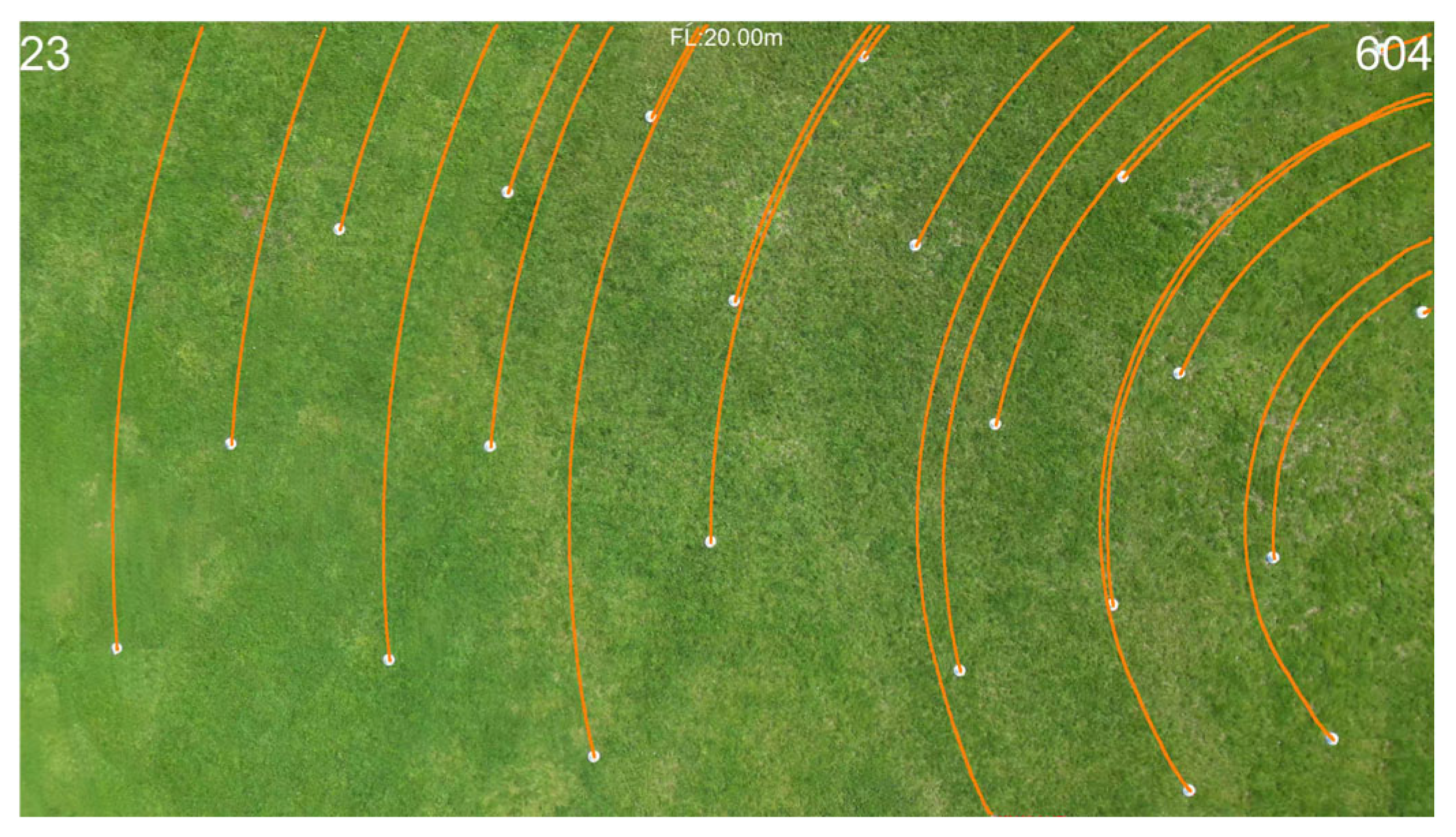
Figure 16 illustrates an example for how the marker trajectories are visualized for this type of motion. It illustrates an example frame from the orbit video captured with flight parameters
= 20 m,
= 5 m/s, and
= 20 degrees/s.
4.9.2. Ramp
This motion is a combination of translational and elevational motion. At a starting flight level of 1 = 5 m, the drone starts moving forward and reaches its target translational speed. At a fixed waypoint in its flight plan, it starts ascending with a fixed elevational rate and keeps on going till a desired flight level 2 is reached. During this ramp up motion, it turns on its camera and captures video.
The drone moves in a forward direction, not sideways. The translational velocity and the elevational rate of the drone are constant. The camera looks forward, and it is downward-facing, i.e., the camera is positioned at −90 degrees with respect to the horizon.
Four different videos with the following flight parameters are captured:
2 m/s, 1 m/s;
4 m/s, 2 m/s.
The flight plan over the marked terrain is prepared and verified as described earlier.
Figure 17 illustrates the aerial and 3D views of it.
Figure 18 illustrates an example for how the marker trajectories are visualized for this type of motion. It illustrates an example frame from the ramp video captured with flight parameters
= 4 m/s and
= 2 m/s. In this frame, the drone is at flight level 21.70 m and ascending.
4.9.3. Helix
This motion is a combination of all of the basic motion types: translational, rotational, and elevational motion at the same time. The drone starts performing an orbit motion but also starts ascending.
The drone moves in a forward direction, not sideways. The translational velocity, the rotational rate, and the elevational rate of the drone are constant. The camera looks forward, and it is downward-facing, i.e., the camera is positioned at −90 degrees with respect to the horizon.
Six different videos with the following flight parameters are captured:
5 m/s, 15 deg/s, 1 m/s;
3 m/s, 10 deg/s, 0.5 m/s.
The flight plan over the marked terrain is prepared and verified as described earlier.
Figure 19 illustrates the aerial and 3D views of it.
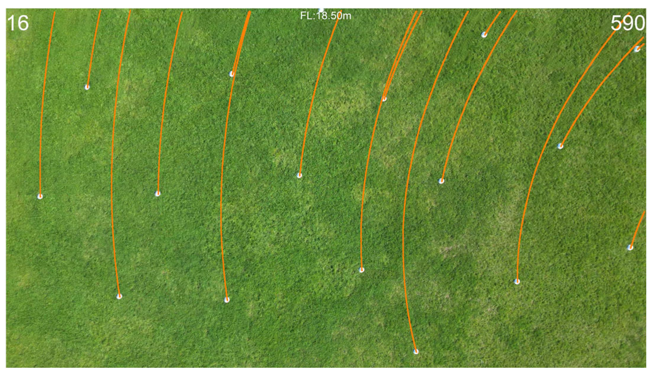
Figure 20 illustrates an example for how the marker trajectories are visualized for this type of motion. It illustrates an example frame from the helix type video captured with flight parameters
5 m/s,
15 deg/s, and
1 m/s. In this frame, the drone is at flight level 18.50 m.
Those complex motion videos are processed with our OpenCV-based utility as described previously, positions of the markers are detected, and actual motion vectors for the markers for the temporal distances of 5 and 25 frames are calculated.
Afterwards, using the positions of the markers, the motion vectors are calculated by utilizing the complex motion model we built in (11).
The difference between the actual motion vectors and the calculated ones is our error rate, thus a direct indication of how successful our final complex motion model is. The results for the basic and complex motion types are evaluated in the following section.
