Article

Integration of Field Data and UAV Imagery for Coffee Yield Modeling Using Machine Learning

by
Sthéfany Airane dos Santos Silva
1,
Gabriel Araújo e Silva Ferraz
2,
Vanessa Castro Figueiredo
1,
Margarete Marin Lordelo Volpato
1,
Danton Diego Ferreira
2,
Marley Lamounier Machado
1,
Fernando Elias de Melo Borges
2 and
Leonardo Conti
3,*
1
Empresa de Pesquisa Agropecuária de Minas Gerais, Av. José Cândido da Silveira, 1647-Bairro União, Belo Horizonte 31170-495, MG, Brazil
2
School of Engineering, Universidade Federal de Lavras, Lavras 37203-202, MG, Brazil
3
Department of Agricultural, Food, Environment and Foresty (DAGRI), University of Florence, 50145 Florence, Italy
*
Author to whom correspondence should be addressed.
Drones 2025, 9(10), 717; https://doi.org/10.3390/drones9100717
Submission received: 7 August 2025 / Revised: 1 October 2025 / Accepted: 10 October 2025 / Published: 16 October 2025

Abstract

The integration of machine learning (ML) techniques with unmanned aerial vehicle (UAV) imagery holds strong potential for improving yield prediction in agriculture. However, few studies have combined biophysical field variables with UAV-derived spectral data, particularly under conditions of limited sample size. This study evaluated the performance of different ML algorithms in predicting Arabica coffee (Coffea arabica) yield using field-based biophysical measurements and spectral variables extracted from multispectral UAV imagery. The research was conducted over two crop seasons (2020/2021 and 2021/2022) in a 1.2-hectare experimental plot in southeastern Brazil. Three modeling scenarios were tested with Random Forest, Gradient Boosting, K-Nearest Neighbors, Multilayer Perceptron, and Decision Tree algorithms, using Leave-One-Out cross-validation. Results varied considerably across seasons and scenarios. KNN performed best with raw data, while Gradient Boosting was more stable after variable selection and synthetic data augmentation with SMOTE. Nevertheless, limitations such as small sample size, seasonal variability, and overfitting, particularly with synthetic data, affected overall performance. Despite these challenges, this study demonstrates that integrating UAV-derived spectral data with ML can support yield estimation, especially when variable selection and phenological context are carefully addressed.

1. Introduction

Coffee cultivation is a major agricultural activity, particularly in developing countries, where it provides livelihoods for millions of producers [1]. In Brazil, the world’s largest coffee producer and exporter, coffee remains central to agricultural exports and rural economies [2,3]. Beyond its economic importance, the main challenge for coffee farming lies in the strong spatiotemporal variability of yield, influenced by biennial cycles, water availability, nutrient status, pests, and diseases [4,5,6,7,8]. Accurate yield forecasting is therefore essential to support farm management, public policies, and market strategies [5].
Recent advances in artificial intelligence (AI) have created new opportunities to address this challenge. Machine learning (ML) algorithms can process large and heterogeneous datasets, including soil attributes, plant physiology, climatic conditions, and spectral information uncovering nonlinear relationships often overlooked by traditional statistical methods [9]. When combined with high-resolution remote sensing, these models can provide spatially explicit yield predictions, enhancing precision agriculture [10,11,12,13]. Their performance, however, may be limited by factors such as small sample sizes, feature selection, and the risks of overfitting or class imbalance, which require careful methodological design.
Among remote sensing tools, unmanned aerial vehicles (UAVs) equipped with multispectral sensors provide high-resolution data closely linked to crop physiology and vigor. Vegetation indices and structural traits such as plant height and canopy diameter are sensitive to nutritional and water conditions, serving as early yield indicators. In perennial crops like coffee, where field measurements are labor-intensive and spatially restricted, UAVs offer a practical and scalable means of consistent data collection throughout the production cycle.
Several studies have explored the use of ML for coffee yield prediction based on satellite imagery [14,15,16], climatic variables [17,18,19,20,21], soil attributes [22,23], management practices [20,21], or UAV-derived traits such as canopy dimensions and vegetation indices [24]. These works demonstrate the value of ML as a decision-support tool in coffee farming. However, few studies have integrated field-based biophysical measurements with high-resolution UAV multispectral data into a structured ML workflow, particularly at the plant level.
To address this gap, the objective of this study was to evaluate the effectiveness of different ML algorithms for coffee yield prediction under three scenarios: (i) using all available variables, (ii) applying feature selection, and (iii) combining feature selection with synthetic oversampling. Five machine learning algorithms, Random Forest (RF), Gradient Boosting (GB), Multilayer Perceptron (MLP), k-Nearest Neighbors (KNN), and Decision Tree (DT), were systematically compared across the three scenarios. This approach enabled the assessment of algorithm robustness and performance in coffee yield prediction using UAV multispectral imagery integrated with field data. Figure 1 summarizes the methodological framework adopted in this study.

2. Materials and Methods

2.1. Characterization of the Study Area, Grid, and Sampling

This study was conducted in an experimental coffee plantation of the Agricultural Research Corporation of Minas Gerais (EPAMIG), located in the municipality of Três Pontas, in the southern region of Minas Gerais, Brazil. The experimental area is situated at an altitude of 905 m, with UTM coordinates S 7640030.4 and E 449531.5. The region has an average annual temperature of 20.3 °C and an average annual rainfall of 1429 mm, and is classified as Cwb (humid subtropical with dry winters and mild summers) according to Köppen’s climate classification [25]. The soil in the area is classified as a Red Latosol (Oxisol) according to the Brazilian Soil Classification System [26].
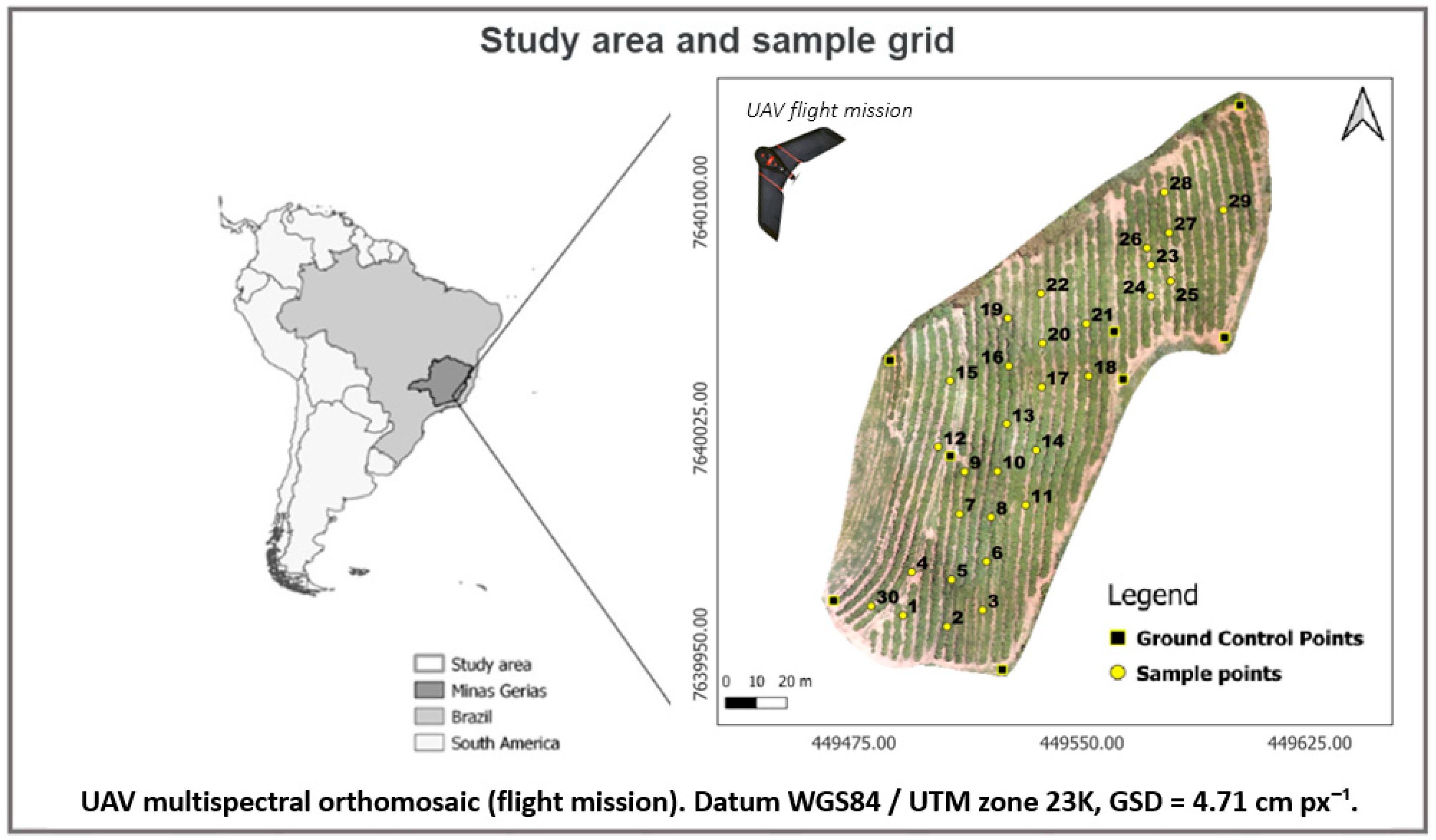
The plantation covers 1.2 hectares and consists of Coffea arabica L. plants, cultivar Topázio MG1190 [27], established in 1998 with a spacing of 3.70 m between rows and 0.70 m between plants. For this study, a sampling grid of 30 georeferenced points was developed using QGIS software (version 3.22.9) (Figure 2), corresponding to a density of 25 points per hectare. The area boundary and point coordinates were obtained using a Trimble R8 RTK GNSS receiver. Each sampling point corresponded to an individual plant, which was identified and monitored throughout the experiment.
After georeferencing the sampling points, two groups of variables were collected to form the dataset used to develop coffee yield prediction models: (i) biophysical variables, obtained through direct field measurements, including yield, soil moisture, leaf water potential, soil fertility, and leaf nutrition; and (ii) spectral variables, derived from multispectral imagery acquired by a Remotely Piloted Aircraft (UAV), comprising vegetation indices, canopy diameter, plant height, and leaf area index (LAI). A summary of all measured variables, including their classification, units, acquisition methods, and sampling periods, is presented in Table 1. A detailed description of the procedures used for data collection and processing is provided in the following subsections.

2.2. Yield

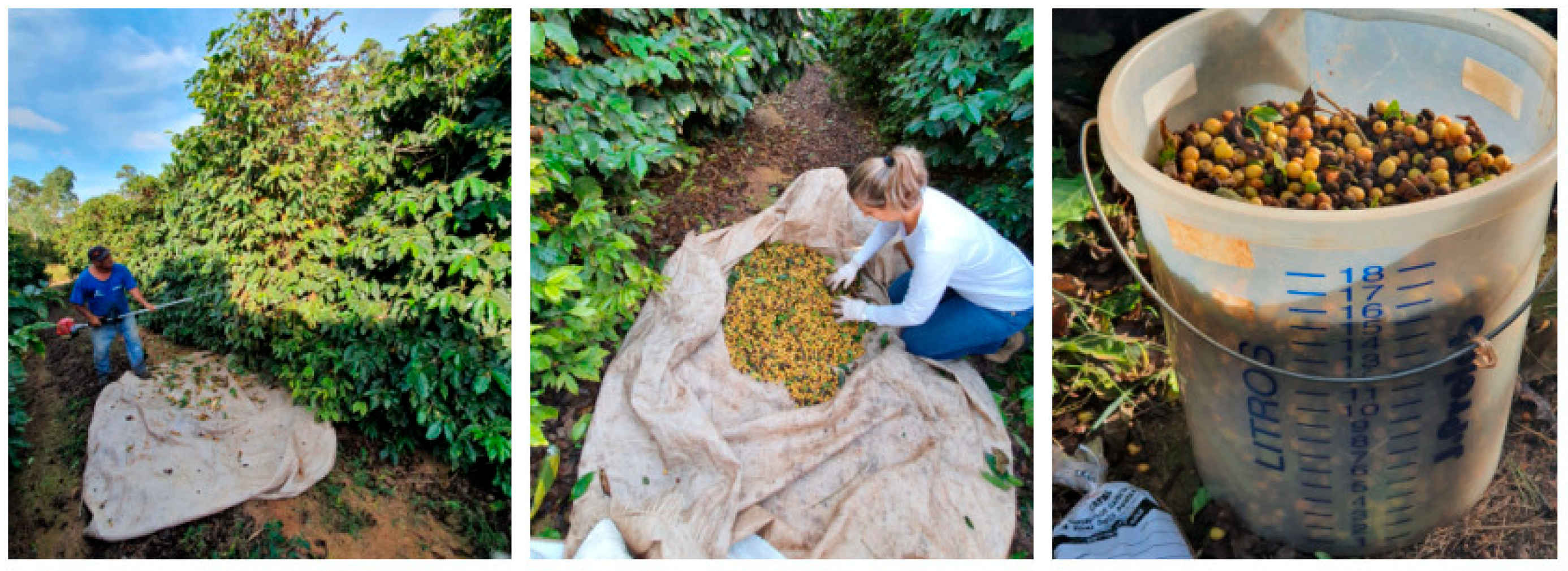
The sampling was carried out in June of each crop season (2020/2021 and 2021/2022) at the 30 georeferenced points in the experimental area. Each sampling point corresponded to a coffee plant, which was harvested using a semi-mechanized method with the assistance of a handheld mechanical harvester. After detachment, the fruits were collected on cloths laid on the ground, followed by manual removal of impurities such as leaves and branches. The cleaned fruits were then placed in a graduated container to estimate yield in liters per plant (Figure 3).

2.3. Soil Moisture

Gravimetric soil moisture (GM) was determined by collecting undisturbed soil samples from a depth of 0–20 cm using an auger. Sampling was carried out on the following dates:
  • 2020/2021 season: August 2020 (dry period) and January 2021 (wet period);
  • 2021/2022 season: August 2021 (dry period) and January 2022 (wet period).
Each sample was collected at pre-established georeferenced points, stored in labeled plastic bags according to the numbering of the sampling points, and then sent to the laboratory for analysis.
Gravimetric moisture was determined using the oven-drying method, following the Brazilian standard NBR 6457/2016 [29]. The samples were first weighed to obtain the wet mass and then dried in an oven at 105 °C for 24 h. After drying, the samples were weighed again to determine the dry mass. These values were used to calculate gravimetric moisture according to Equation (1).
θ g = M w a t e r M d r y = M w e t M d r y M d r y θ g % = θ g 100
where
  • M w e t = mass of the wet soil sample (g)
  • M d r y = mass of the dry soil sample (g)

2.4. Water Potential

Leaf water potential (Ψw) was measured using a Scholander-type pressure chamber [30], an instrument designed to assess xylem sap tension. Sampling was performed on the same dates as the soil moisture measurements: August 2020 and January 2021 for the 2020/2021 season, and August 2021 and January 2022 for the 2021/2022 season.
In this study, Ψw values were obtained during the early morning hours (between 04:00 and 06:00), known as predawn water potential. This measurement is commonly used as an indicator of soil water availability, as it tends to reflect the equilibrium between plant and soil water status under non-severe water deficit conditions [31].
At each georeferenced point, three leaves were collected from the middle third of the plant, between the third and fourth leaf pairs, with intact petioles. After collection, the leaves were properly labeled and stored to prevent moisture loss.
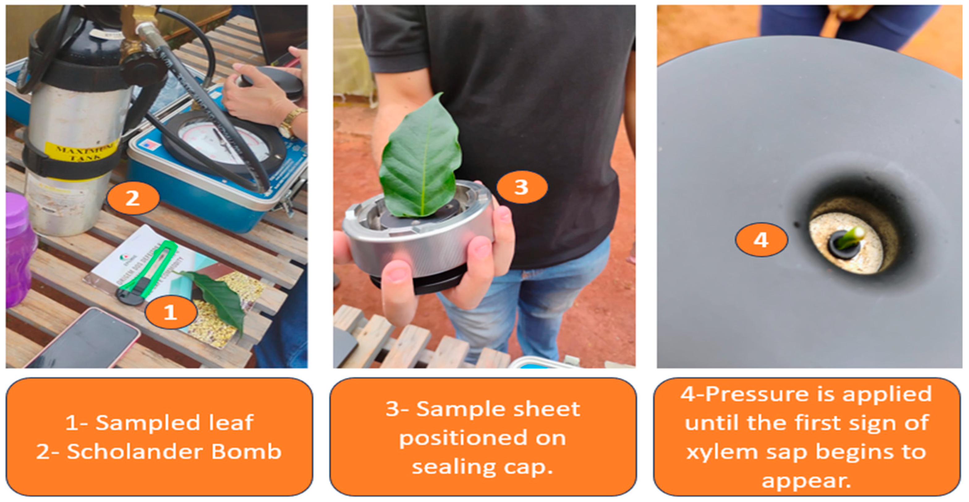
The samples were then analyzed using the Scholander pressure chamber (Figure 4). The method involves placing the leaf inside a sealed cylinder, leaving only the petiole exposed through a gas-tight rubber seal. Pressure is gradually applied until the first appearance of sap at the cut surface of the petiole. At that point, the flow of inert gas (nitrogen) is stopped, and the pressure reading on the manometer is recorded. This value represents the xylem pressure potential, expressed in MPa (megapascals).

2.5. Soil Fertility and Leaf Nutrition Analysis

The nutritional status of the plants was evaluated through soil fertility and leaf nutrient analyses to investigate their relationship with coffee yield. Soil samples were collected in April 2021 and April 2022 at the same 30 georeferenced points used for the other variables, from a depth of 0–20 cm, and sent to a specialized laboratory. The analyses included phosphorus (P), remaining phosphorus (Prem), potassium (K), calcium (Ca), magnesium (Mg), pH, organic matter (OM), and total acidity (H + Al).
Leaf sampling was carried out during the “chumbinho” stage of fruit development, between December and mid-January. At each point, 50 leaves were taken from the reference plant and neighboring plants, always from the middle third of the canopy, between the third and fourth leaf pairs. Only healthy leaves without signs of disease, nutrient deficiency, climatic damage, or mechanical injury were selected. These samples were then analyzed in a laboratory for the concentrations of N, P, K, Ca, Mg, S, Mn, Zn, B, Cu, and Fe.
For this study, leaf nutrient analysis was performed only for the 2021/2022 crop season.

2.6. High Resolution Imagery

High-resolution multispectral imagery was central to this study, enabling the extraction of spatial and spectral variables directly linked to plant physiology and productivity. The UAV-based approach provided timely, non-destructive, and scalable data acquisition, which was integrated into the predictive modeling framework.
Flights were carried out with a Remotely Piloted Aircraft (UAV) equipped with a Parrot Sequoia (Parrot Drones SAS, Paris, France) multispectral sensor, conducted simultaneously with soil moisture and leaf water potential measurements in August 2020, January 2021, August 2021, and January 2022. The dates were chosen to represent two contrasting phases of the coffee production cycle: the dry season (August) and the rainy season (January). This schedule aligned with the objectives of the broader research project, which focused on assessing plant water status and water stress. Acquiring imagery during these phenological stages allowed us to capture temporal variations in plant physiology and soil moisture. Although the flights did not coincide with harvest, the multispectral data collected at these stages provided robust indicators of plant vigor and development, which are strongly associated with final yield.
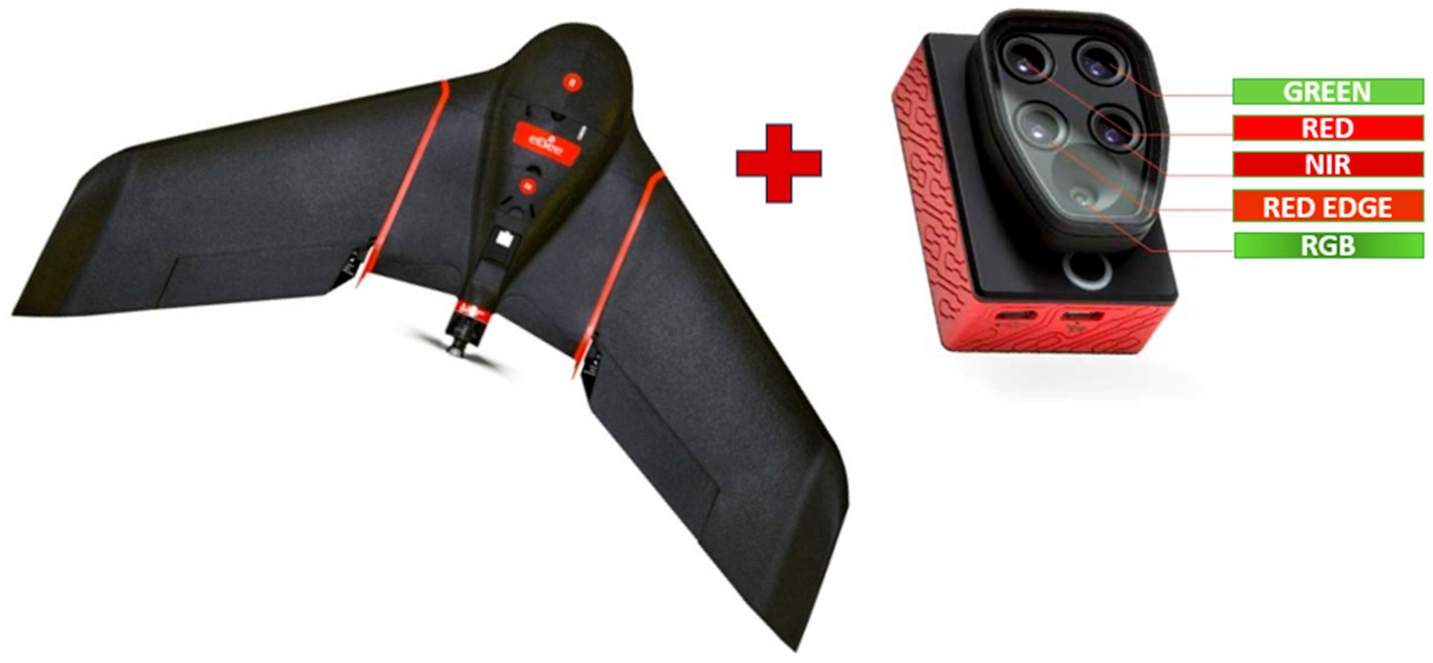
The aircraft used was an eBee SQ (senseFly SA, Cheseaux-sur-Lausanne, Switzerland, Figure 5), a fixed-wing platform with a 110 cm wingspan, 3 km nominal radio range, cruising speed of 40–110 km/h, wind resistance up to 45 km/h (12 m/s), electric motor, and maximum payload of 1.1 kg (including camera and batteries). Its flight autonomy was up to 55 min.
Flight planning and execution were managed through the aircraft’s dedicated base station and eMotion software (version 3.5), which defined flight routes, altitude, ground sampling distance, and image overlap. The UAV operated with an integrated autopilot combining GNSS RTK positioning and an inertial measurement unit (IMU), ensuring stable flight attitude and high-accuracy trajectory control. A transmitter antenna enabled real-time monitoring and allowed command inputs for landing, course adjustments, and image capture. The interface displayed key flight parameters, including battery level, ambient temperature, altitude, flight duration and speed, wind speed, image resolution, longitudinal and lateral overlap, and radio link quality. This integrated system ensured precise and consistent image acquisition, going beyond simple GPS-based navigation.
The flight parameters were as follows:
  • Focal length: 3.98 mm;
  • Vertical overlap: 70%;
  • Horizontal overlap: 70%;
  • Flight altitude: 50 m;
  • Ground sampling distance (GSD): 4.71 cm px−1;
  • Speed: 12 m/s;
  • Estimated flight time: 10 min.
The Parrot Sequoia sensor captures five spectral bands:
  • Green (550 nm ± 40 nm);
  • Red (660 nm ± 40 nm);
  • RedEdge (735 nm ± 10 nm);
  • Near-infrared–NIR (790 nm ± 40 nm);
  • RGB (visible band–420–700 nm).
The images acquired by the sensor were processed using Pix4DMapper software (version 4.4.10). The workflow included image block phototriangulation to determine internal and external orientation parameters, point cloud generation, creation of the Digital Surface Model (DSM), and orthomosaic generation. For phototriangulation, eight ground control points (GCPs) were strategically distributed across the experimental area and surveyed with a Trimble R8 GNSS (Trimble Inc., Sunnyvale, CA, USA) receiver operating in RTK (Real Time Kinematic) mode, dual frequency, and sub-millimeter precision (<1 mm at 1 Hz).
Radiometric correction of the orthomosaics was performed to convert digital number (DN) values to surface reflectance. This was performed in Pix4DMapper using the Parrot Sequoia sensor’s calibration tools. A reflectance panel was used before each flight to calibrate the camera, enabling the software to adjust reflectance values according to illumination conditions at the time of image acquisition.
This step ensured the spectral consistency of the dataset across all acquisition dates, reducing variability caused by atmospheric and lighting conditionsan essential requirement for quantitative vegetation index analysis.
The final products included orthomosaics for the Green, Red, RedEdge, and NIR bands, an RGB orthomosaic, and both a Digital Terrain Model (DTM) and a Digital Surface Model (DSM). These processed outputs formed the basis for calculating vegetation indices and structural metrics.

2.6.1. Vegetation Index

To explore the information derived from the multispectral imagery, vegetation indices were calculated for each point in the sampling grid. Values were extracted from the pixels contained within the polygons corresponding to the georeferenced sampling points. Using the NIR, Red, and RedEdge bands, the following spectral vegetation indices were calculated (Table 2).
The vegetation indices were calculated in QGIS software using the Raster Calculator tool. After each index was calculated, a shapefile was created containing 30 polygons with a diameter of 30 cm, representing the georeferenced sampling points within the study area.
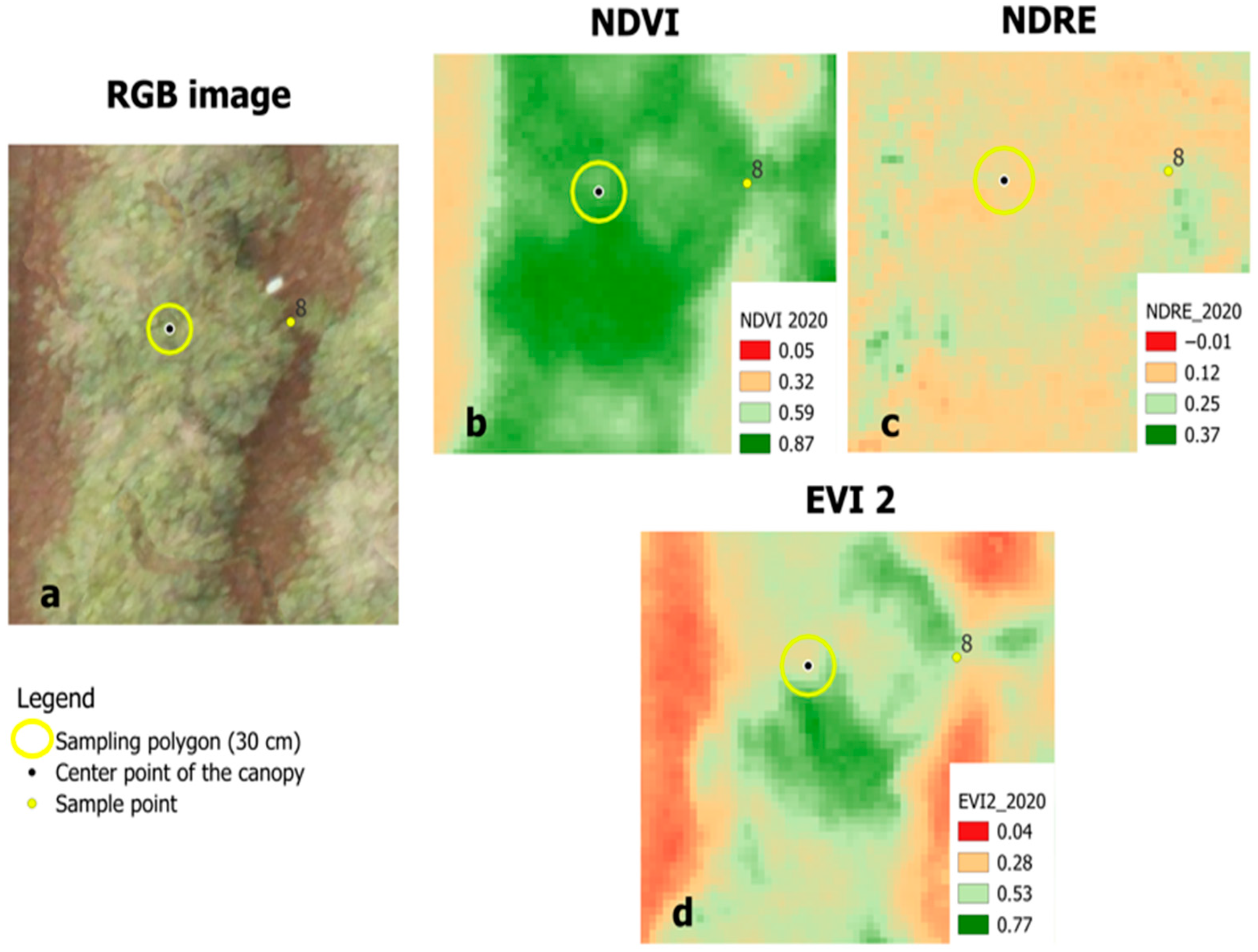
The adoption of a 30 cm polygon was based on previous studies conducted in the same experimental coffee field, where smaller sampling areas (20 cm in diameter) were successfully used to extract vegetation indices from UAV multispectral imagery [35,36]. These studies showed that compact canopy-centered polygons effectively reduce interference from exposed soil, shading, and weeds while preserving the spectral representativeness of the coffee canopy. In the present study, the 30 cm polygon was chosen because it encompassed only the pixels corresponding to the canopy of the sampled plants, as illustrated in Figure 6. Building on the methodological consistency of earlier works, the slightly larger diameter (30 cm) was adopted to increase the number of pixels per polygon, thereby improving the robustness of spectral averaging without compromising canopy specificity.
Based on these polygons, vegetation index values were extracted using the Zonal Statistics tool in QGIS. This tool calculates the average pixel values within each polygon. As a result, for each vegetation index, 30 mean values were generated for each sampling point in the grid.

2.6.2. Plant Height, Canopy Diameter, and Leaf Area Index of Coffee Plants

Plant height (H) estimates derived from UAV imagery followed the workflow described by [37], where height is calculated as the difference between the Digital Surface Model (DSM) and the Digital Terrain Model (DTM), as shown in Equation (2). Pixel values from the digital models were distinguished using the point sampling tool.
H i = D S M   x i ,   y i D T M   ( x i ,   y i )
where
  • Hi: plant height estimated at sampling point i (m)
  • DSM (xi, yi): value of the Digital Surface Model at pixel (xi, yi) (m)
  • DTM (xi, yi): value of the Digital Terrain Model at the same pixel (xi, yi) (m)
Canopy diameters were estimated following the methodology proposed by [24]. After exporting the RGB orthomosaic to QGIS software, the average canopy diameter for each sampled plant was manually obtained using bounding boxes.
The Leaf Area Index (LAI) was calculated using the non-destructive method described by [28], based on the canopy diameter (D) and plant height (H), as defined in Equation (3).
L A I = 0.0134 + 0.7276 × D 2 × H

2.7. Feature Selection

Correlation analysis was applied as a feature selection technique to evaluate the relationship between the predictor variables (input features) and the target variable (yield). This approach allows predictive models to be built using only the variables with the strongest influence on yield, reducing model complexity and avoiding high dimensionality, particularly when the number of variables exceeds the number of available samples [38].
Pearson’s correlation was used as the statistical measure to quantify the linear relationship between two numerical variables. Its coefficient, known as Pearson’s Correlation Coefficient (R), ranges from −1 to 1 and is calculated as shown in Equation (4).
R = ( X i X ^ ) ( Y i   Y ^ ) X i X ^ 2 ·   ( Y i   Y ^ ) 2
where
  • R = correlation coefficient;
  • X i = values of the independent variables (soil moisture, leaf water potential, soil fertility, leaf nutrient and spectral variables);
  • X ^ = mean of the independent variables;
  • Y i   = values of the dependent variable (coffee yield);
  • Y ^ = mean of the dependent variable.
The interpretation of Pearson’s correlation coefficient (R) is as follows:
  • R = 1 → perfect positive correlation (both variables increase together);
  • R > 0 → positive correlation (high values of X tend to be associated with high values of Y);
  • R = 0 → no linear correlation (no clear linear relationship between the variables);
  • R < 0 → negative correlation (as one variable increases, the other tends to decrease);
  • R = −1 → perfect negative correlation (a perfect inverse linear relationship).
After the correlation analysis, the data were standardized using Z-score normalization, an essential step in machine learning, particularly for algorithms sensitive to the scale of input variables. This method transforms the data so that the mean is zero and the standard deviation is one, ensuring that all variables contribute equally during model training.
To develop the coffee yield prediction models, three distinct datasets were structured. In all scenarios, the dependent variable was coffee yield (in liters per plant). The difference between scenarios lies in the set of independent (predictor) variables used to train the models:
Dataset 1: Full set of variables:
-
Dependent variable: yield;
-
Independent variables: Soil moisture: GH_2020, GH_2021, Leaf water potential (WP_2021, WP_2022), Soil fertility attributes (pH, P, K, Ca, Mg, MO, H + Al), Leaf nutrition 2021/2022 (N, P, K, Ca, Mg, S, Mn, Zn, B, Cu, Fe), Spectral vegetation indices (NDVI, NDRE, EVI2), Plant height, canopy diameter, leaf area index (LAI);
Dataset 2: Variables selected based on correlation with yield:
-
Dependent variable: yield;
-
Independent variables: For the 2020/2021 season (GH_2020, GH_2021, NDRE_2020, pH), for the 2021/2022 season (WP_2022, P_foliar, S_foliar, N_foliar, K_foliar), for the combined seasons (GH_2020, GH_2021, NDVI_2020, NDRE_2020, H + Al);
Dataset 3: Variables selected variables (as Scenario 2) + data augmentation using SMOTE:
-
Dependent variable: yield;
-
Independent variables: same as those used in Scenario 2, but with the dataset artificially expanded using the SMOTE (Synthetic Minority Over-sampling Technique) method. This approach tripled the number of samples in the dataset to improve model training and reduce overfitting caused by the limited original sample size.
The yield data were analyzed using descriptive statistics, including mean, minimum, maximum, standard deviation, skewness, and coefficient of variation (CV).
In this study, multiple regression analyses were carried out with machine learning algorithms to evaluate their ability to generate yield prediction models for coffee crops using a dataset with a limited number of samples. Multiple regression is a statistical technique used to explore and infer the relationship between a dependent variable (response) and a set of independent variables (predictors). In this case, the predictors included soil moisture, water potential, soil fertility, leaf nutrition, plant height, canopy diameter, leaf area index (LAI), and vegetation indices, while yield was the response variable.
To assess model performance, the data were structured into three datasets (Table 3), allowing comparison of prediction effectiveness across the tested configurations.
Based on the dataset obtained in this study, multiple regression analyses were conducted using machine learning algorithms implemented in Python (version 3.12). The objective was to evaluate the ability of these algorithms to predict coffee yield with a limited number of samples.
Multiple regression enables the investigation of the relationship between a dependent variable (yield) and several independent variables, including soil moisture, leaf water potential, soil fertility, leaf nutrition, plant height, canopy diameter, leaf area index (LAI), and vegetation indices.
The models were developed annually using data collected in the year preceding the harvest, incorporating variables related to soil, plant characteristics, and spectral attributes. This approach aimed to produce models that better reflect field conditions, providing relevant information to support producers in planning for the following crop season.
Only manageable variables were considered in this study. However, it is important to recognize that environmental factors such as climate, extreme weather events, precipitation, and inherent soil properties also play a critical role in coffee yield. Although these factors cannot be directly controlled, they interact with management practices and may influence the effectiveness of the adopted strategies.
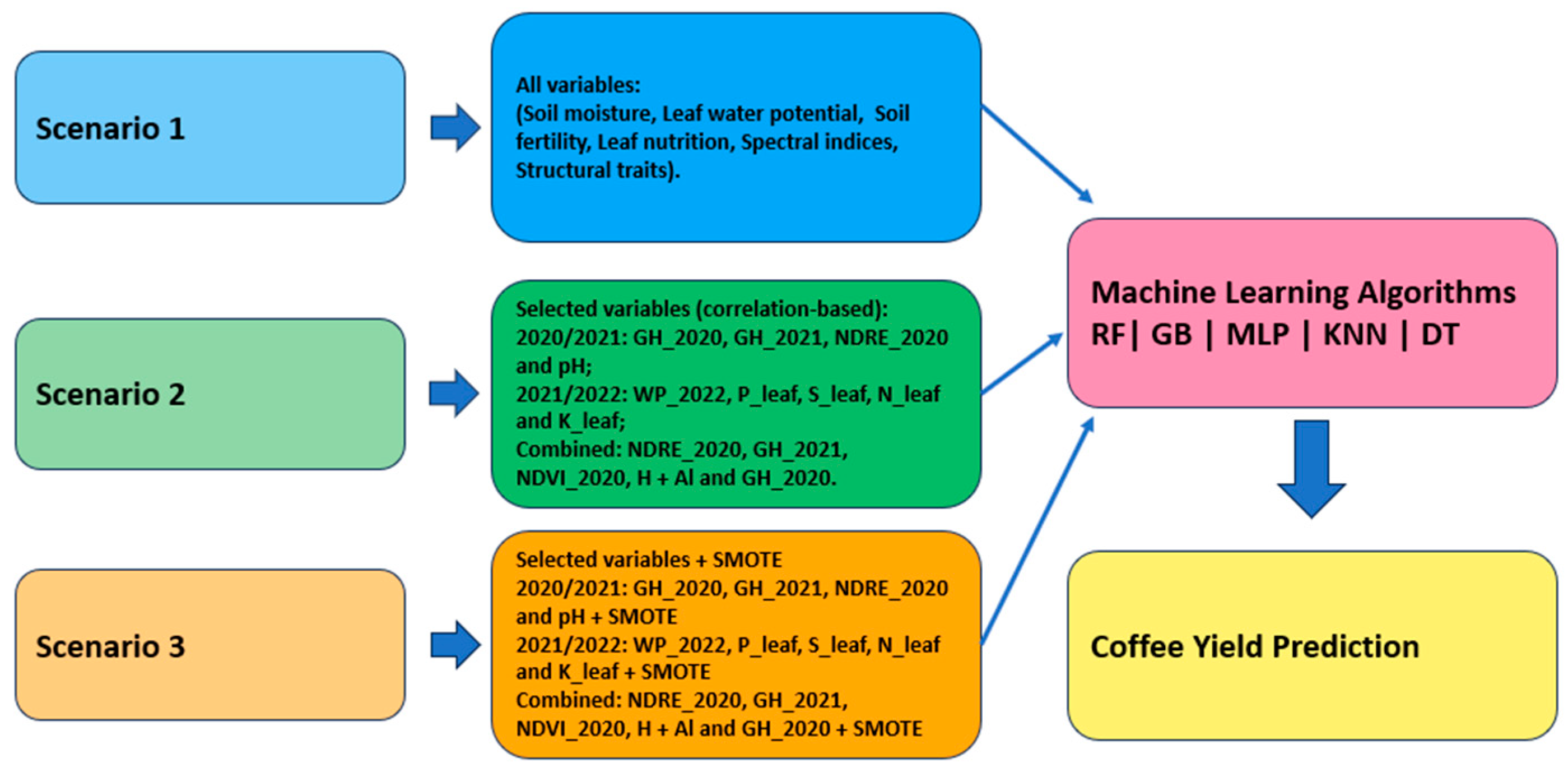
The workflow of the three scenarios and machine learning algorithms is summarized in Figure 7.
The machine learning algorithms used for modeling were Random Forest (RF), Gradient Boosting (GB), Multilayer Perceptron (MLP), K-Nearest Neighbors (KNN), and Decision Tree (DT). These algorithms were chosen because they represent different methodological families, including ensemble learning, instance-based learning, neural networks, and tree-based models. They are commonly used as benchmarks in agricultural prediction studies, ensuring comparability with previous research. Given the limited dataset, algorithms known for stable performance with small samples were prioritized to minimize the risk of overfitting associated with more complex approaches.
Random Forest (RF), developed by [39], is an extension of the Decision Tree (DT) algorithm in which multiple trees are built from subsets of the dataset and their predictions aggregated. RF reduces the risk of overfitting and improves accuracy, although its interpretation is more complex.
Gradient Boosting (GB), proposed by [40], is a supervised learning algorithm based on the boosting technique. It combines multiple weak models, typically decision trees, into a more robust and accurate ensemble.
Multilayer Perceptron (MLP) is a feedforward artificial neural network composed of multiple layers of neurons. Developed by [41], it is widely applied to regression and classification tasks and is one of the most popular models in deep learning.
K-Nearest Neighbors (KNN), introduced by [42], is an instance-based algorithm that makes predictions based on the average of the k nearest neighbors in the feature space. It is simple and effective for small datasets and nonlinear problems, though it can be computationally demanding for larger datasets and sensitive to the choice of k.
Decision Tree (DT), proposed by [43], splits the data space into regions based on binary decisions, forming a tree-like structure. Unlike multiple linear regression, DT does not assume linear relationships and can capture nonlinear patterns. However, if not properly tuned, it is prone to overfitting.

2.8. Validation Prediction Models

When multiple regression analyses are carried out using machine learning algorithms, cross-validation (CV) plays a crucial role in ensuring that the models are robust and generalize well to new data. CV also helps prevent overfitting by ensuring the model captures real patterns rather than simply fitting the training data. This approach provides more reliable estimates of model performance by splitting the data into different subsets for training and testing.
In this study, cross-validation was applied by splitting the dataset into 80% for training and 20% for testing. The validation method used was Leave-One-Out Cross-Validation (LOO-CV), which is particularly recommended for small datasets as it maximizes the use of all available samples during model training.
In LOO-CV, the dataset is divided into n iterations (where n is the total number of observations). In each iteration, a single sample is used as the test set, and the remaining n − 1 samples are used for training. This process is repeated n times, and overall performance is obtained by averaging the results from all iterations. The general formula is:
L O O C V   E r r o r = 1 n i = 1 n L ( y i , y ^ i )
where L (yᵢ, ŷᵢ) is the loss function that compares the actual value yᵢ with the predicted value ŷᵢ for each observation.
As many regression tasks do not follow well-defined linear patterns, two performance metrics were used to evaluate the algorithms:
- Root Mean Squared Error (RMSE): indicates the average prediction error in the same unit as the dependent variable.
R M S E = 1 n i = 1 n y i , y ^ i 2
- M e a n   A b s o l u t e   P e r c e n t a g e   E r r o r   ( M A P E ) : expresses the prediction error in percentage terms, facilitating comparison across models.
M A P E = 100 n i = 1 n y i , y ^ i y i
Note: MAPE was only calculated for samples where yᵢ ≠ 0, since division by zero renders the calculation invalid.
These metrics were calculated for both training and testing sets to assess model performance and generalization ability.

2.9. Statistical Analysis of Model Performance

To assess whether differences among algorithms were statistically significant, a one-way analysis of variance (ANOVA) was performed using the test RMSE values for each scenario and crop season. The null hypothesis assumed that the mean RMSE values of all algorithms were equal, while the alternative hypothesis stated that at least one algorithm differed. Pairwise comparisons with a significance level of p < 0.05 were then applied to identify specific differences among algorithms. This analysis provided a statistical basis for interpreting the comparative performance of the models.

3. Results

3.1. Descriptive Statistic

The dataset related to yield was analyzed for mean, minimum–maximum, standard deviation, skewness, and coefficient of variation (CV), as presented in Table 4.
According to [44], spatial and temporal variability in crop yield is a recurring issue in coffee-growing regions. Beyond differences between neighboring plants, biennial bearing strongly influences production. In high-yield years, the heavy use of a plant’s energy reserves can limit the development of new productive branches, leading to reduced yield in the following cycle [45,46]. The restricted growth of plagiotropic branches, which are responsible for fruiting, further amplifies the alternation between years of high and low production. Biennial bearing also directly affects yield forecasting, making productivity estimation a persistent challenge for growers [47].
In addition to this biennial effect, the productivity drop observed in the 2021/2022 season may have been aggravated by water deficits during flowering or fruit filling, although specific climatic data were not included in this study [48]. The lack of irrigation may also have intensified the negative impact of weather conditions on production.
Although the primary objective of this study was not to analyze yield differences between the evaluated seasons, interpreting the data in light of the variables used in the modeling provides important insights. The decrease in average productivity in the 2021/2022 season (5.47 L plant−1) compared with the previous season (10.20 L plant−1) can be attributed not only to biennial bearing but also to physiological and environmental factors that directly influence crop performance.
Soil moisture and leaf water potential data suggest that plants experienced greater water stress during the 2021/2022 season, particularly in the dry period (August), which may have affected fruit filling. Moreover, fluctuations in the availability of key nutrients such as potassium (K), phosphorus (P), and organic matter, as observed in the soil fertility and leaf nutrition analyses, may have negatively impacted plant development and yield.
Therefore, the decline in yield during the 2021/2022 season appears to have resulted from the interaction of plant physiological factors (such as biennial bearing), reduced water availability, and variations in soil attributes. Considering these aspects is essential for understanding the challenges of yield prediction and reinforces the importance of integrating both biophysical and spectral variables into the development of more robust predictive models.

3.2. Correlation Analysis

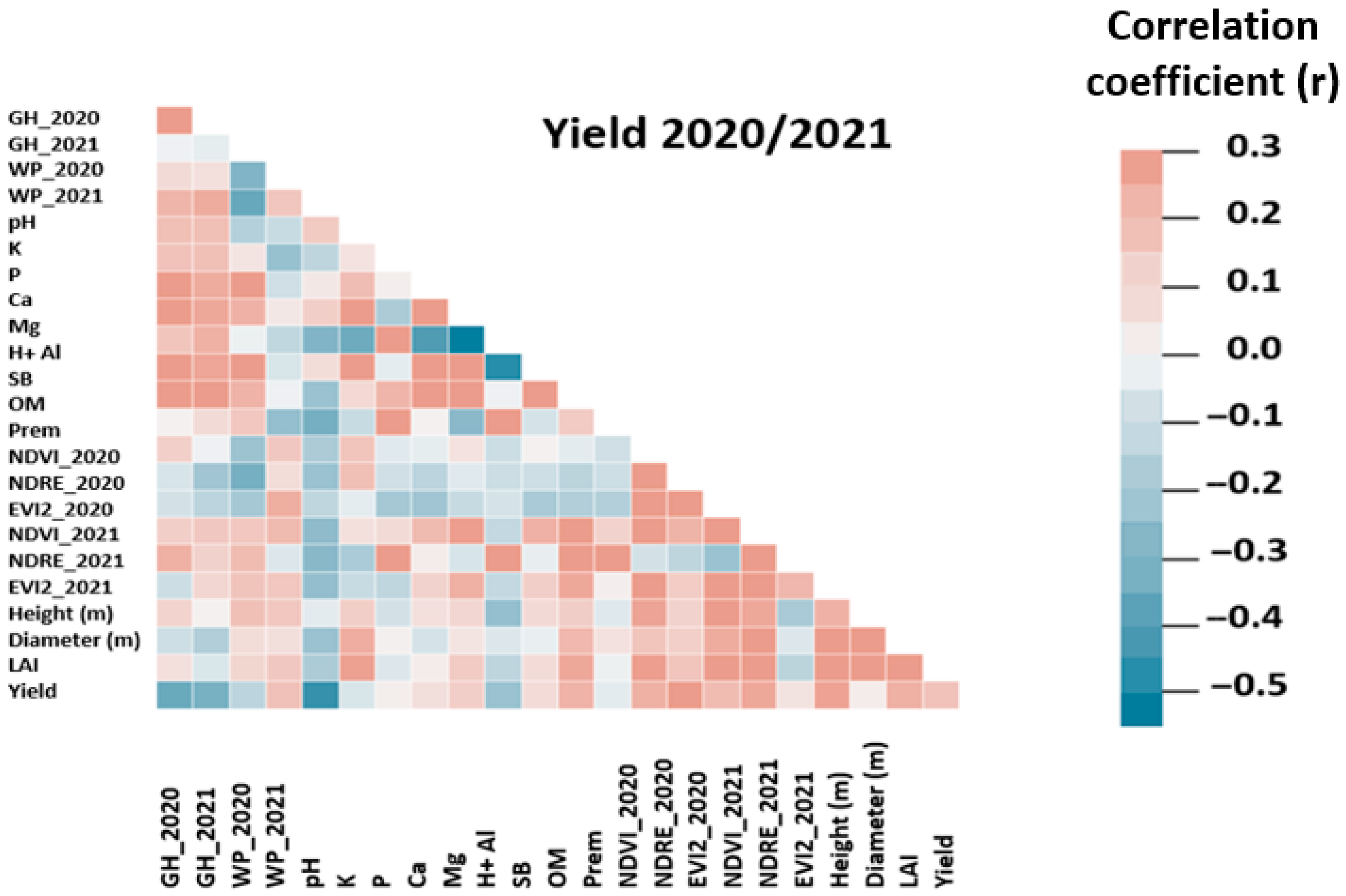
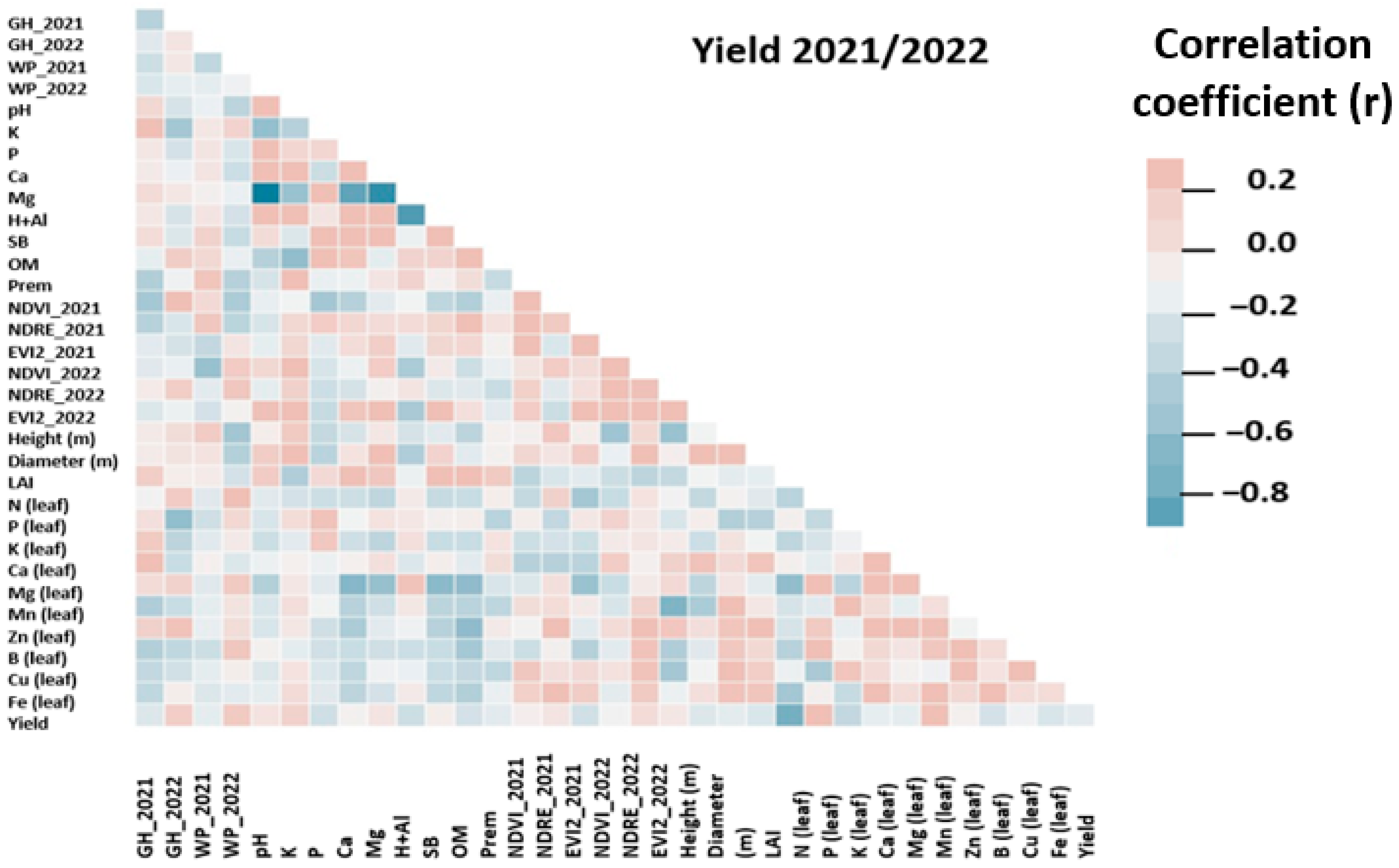
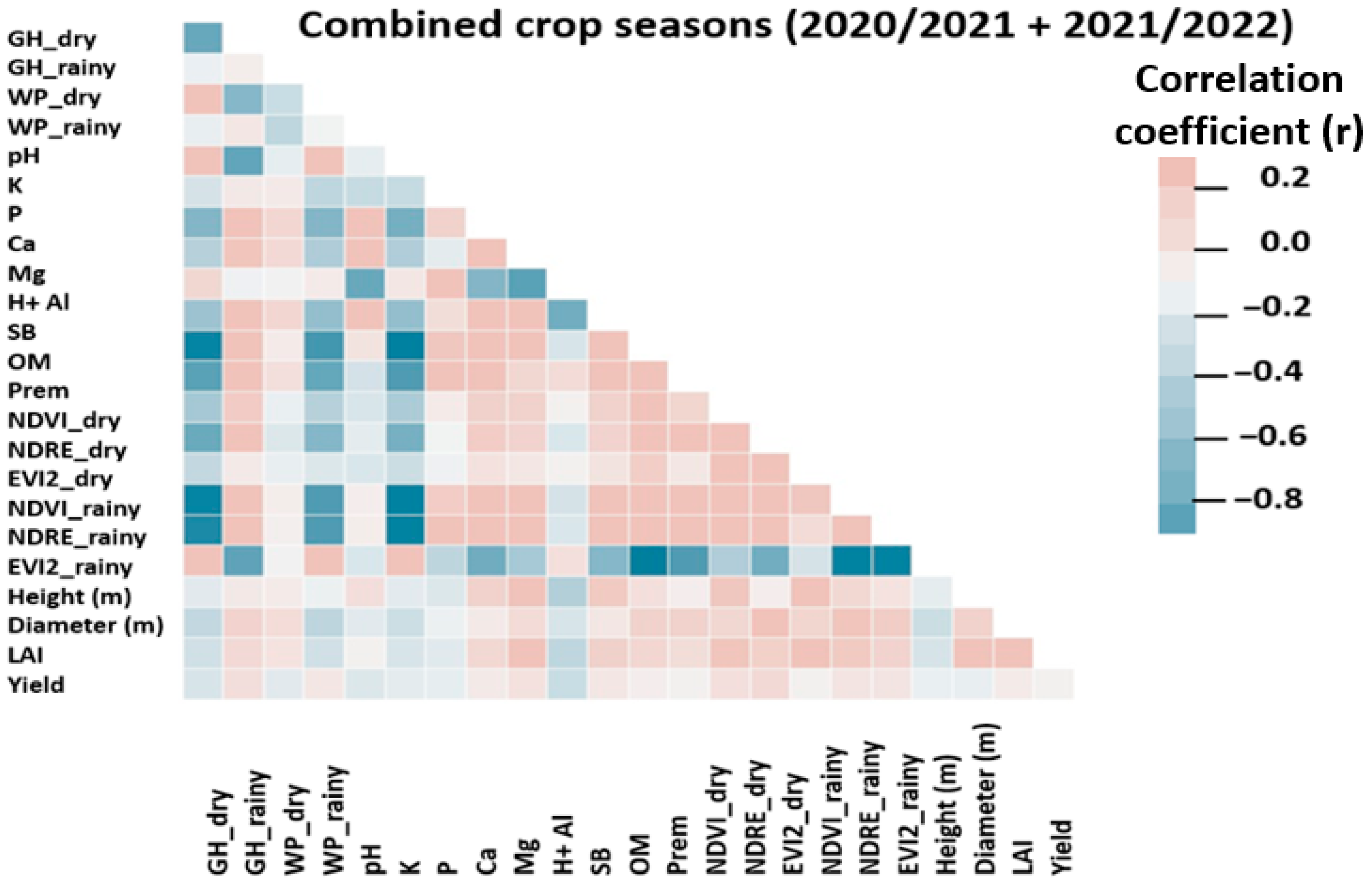
Figure 8, Figure 9 and Figure 10 present the correlation plots corresponding to Scenarios 1, 2, and 3, respectively.
For the 2020/2021 crop season (Figure 8), the selected attributes were GH_2020, GH_2021, pH (negative correlation ranging from 0.3 to 0.5), and NDRE (positive correlation of about 0.3). In other words, the most influential variables in the 2020/2021 dataset were gravimetric soil moisture sampled in August 2020 and January 2021, soil pH, and the NDRE index from August 2020.
For the 2021/2022 crop season (Figure 9), the selected attributes were WP_2022, P_leaf, and S_leaf (positive correlations between 0.2 and 0.4), and N_leaf and K_leaf (negative correlations of about 0.5 for N and 0.2 for K). In this season, foliar nutrition variables showed a stronger correlation with yield, along with leaf water potential values collected in January 2022.
In the combined dataset (Figure 10), correlations between attributes and yield were weaker. The selected attributes were NDRE_2020, GH_2021, NDVI_2020, H + Al, and GH_2020, with positive correlations of about 0.1 to 0.2.

3.3. Prediction Models

Table 5, Table 6 and Table 7 present the RMSE and MAPE values from the training and testing sets for each algorithm, corresponding to Scenario 1 (Table 5), Scenario 2 (Table 6), and Scenario 3 (Table 7).
Because the dataset included georeferenced points with zero yield (0 L/plant) and Leave-One-Out cross-validation was applied where each iteration uses only one sample for testing, some MAPE values could not be calculated. This occurs because the MAPE formula uses the actual yield (yi) as the denominator, and when yi = 0, yi = 0, the fraction is undefined, making the metric invalid.

3.3.1. Algorithm Performance for Scenario 1 (Original Dataset)

A comparative analysis of the RF, GB, MLP, KNN, and DT algorithms, presented in Table 5, revealed clear differences in predictive performance across the 2020/2021 and 2021/2022 seasons based on RMSE and MAPE metrics.
In the 2020/2021 season, KNN outperformed the other models in the test set, achieving the lowest RMSE (4.21 L/plant) and MAPE (2.51%), indicating strong accuracy in both absolute and relative terms. By contrast, DT showed the weakest performance, with the highest RMSE (13.06 L/plant) and MAPE (6.16%), reflecting poor predictive ability and weak model fit.
In the 2021/2022 season, RF achieved the lowest RMSE in the test set (8.59 L/plant), suggesting it was more effective in capturing yield variability under that season’s conditions. KNN again performed well, showing the lowest MAPE in the training set (2.27%). DT continued to perform poorly, with high test RMSE (15.41 L/plant) and training MAPE (6.41%), confirming its limited generalization capacity. GB also had a relatively high RMSE (13.66 L/plant), indicating reduced robustness for this season.
When the two seasons were combined, RF once again stood out, achieving the lowest test MAPE (0.98%) and a relatively low RMSE (11.11 L/plant), indicating better generalization across the full dataset. In contrast, DT continued to show the weakest performance, with the highest RMSE (13.35 L/plant) and MAPE (1.71%) in the test set, reaffirming its inadequacy for yield prediction in this context.
Overall, across all seasons, DT consistently underperformed, suggesting it is not well-suited to the complexity or variability of the original dataset. By comparison, KNN showed better accuracy with raw data, while RF demonstrated greater stability and generalization, especially when combining data across multiple seasons.

3.3.2. Algorithm Performance for Scenario 2 (Selected Variables)

Based on the results in Table 6, the five regression algorithms showed considerable variation in performance across the analyzed crop seasons.
In the 2020/2021 season, KNN achieved the lowest training error (4.51 L/plant), followed by MLP (4.72 L/plant), indicating a better fit to the training data. In the test set, MLP performed best, with the lowest RMSE (1.78 L/plant) and the second-lowest MAPE (0.74%). DT had the weakest performance, with a test RMSE of 6.20 L/plant and a training RMSE of 3.02 L/plant, suggesting it was not well suited to this dataset.
In the 2021/2022 season, KNN again showed the lowest training error (RMSE = 6.77 L/plant), followed by RF (6.92 L/plant). In the test set, GB achieved the best result (RMSE = 9.14 L/plant). DT once again performed worst, with a test RMSE of 15.92 L/plant, indicating low predictive accuracy.
For the combined dataset (2020/2021 + 2021/2022), KNN produced the lowest training RMSE (6.30 L/plant), followed by RF (6.97 L/plant). In the test set, RF and KNN tied with the lowest RMSE (5.26 L/plant), followed by MLP (5.34 L/plant), which also had the lowest MAPE (1.80%). DT continued to show the weakest performance, with a training RMSE of 8.41 ± 9.41, a test RMSE of 10.88 L/plant, and a MAPE of 3.79%, indicating it was unable to adequately model the combined dataset.

3.3.3. Algorithm Performance for Scenario 3 (Selected Variables + SMOTE)

In the 2020/2021 season, RF and GB showed the lowest RMSE values in the test set (2.09 and 2.28 L/plant, respectively), indicating strong absolute performance. DT recorded the lowest MAPE (0.67%) in the test set, suggesting its predictions were the most accurate in relative terms. KNN showed the largest gap between training and test RMSE (+3.40 L/plant), indicating potential underfitting. DT had an extremely low RMSE during training (0.90 L/plant), followed by a sharp increase in the test set (+2.24 L/plant), pointing to possible overfitting.
In the 2021/2022 season, all models experienced a substantial increase in test RMSE, indicating severe overfitting. KNN had the largest increase (+14.49 L/plant), suggesting excessive fitting to the training data. RF achieved the lowest test RMSE (9.04 L/plant), though the value was still relatively high, reflecting poor generalization.
In the combined dataset, MLP achieved the lowest test RMSE (5.61 L/plant), showing the best absolute prediction performance, and also recorded the lowest test MAPE (2.26%). DT exhibited a large increase in test RMSE (+9.16 L/plant), again suggesting overfitting. RF and GB remained more stable but still showed higher absolute errors.
The application of the SMOTE technique led to a notable reduction in training errors across all scenarios, as expected from dataset balancing and augmentation. However, this improvement was not consistent in the test results. In the 2020/2021 season, SMOTE improved model performance by substantially lowering test RMSE compared with previous scenarios. In contrast, in the 2021/2022 season, test errors increased sharply, indicating strong overfitting. In the combined dataset, test RMSE values also rose, though less markedly. Thus, SMOTE proved more beneficial in the 2020/2021 season but showed limited effectiveness in the other contexts.
The use of synthetic data generation techniques such as SMOTE (Synthetic Minority Oversampling Technique) may also introduce bias, as interpolating between nearby minority samples can create unrealistic instances, distort class boundaries, or reinforce limited representations of the minority class. These issues may lead models to learn artificial patterns or overestimate performance. To reduce such risks, SMOTE should be applied only to the training set, and more robust variants (e.g., Borderline-SMOTE, ADASYN) or hybrid approaches with data cleaning can be considered. Additionally, complementing synthetic augmentation with real data collection and careful validation is essential to ensure fairness and generalization [48,49,50].

3.3.4. Comparative Analysis of Modeling Scenarios

When comparing the three evaluated scenarios, the following observations can be made:
(a) 2020/2021 Season:
Scenario 1—Original dataset: showed the highest RMSE values in the test set, with the DT model reaching a high error of 13.06 L/plant, indicating extreme overfitting.
Scenario 2—Selected variables: significantly improved results. RMSE values dropped below 3.5 L/plant for all models, with MLP achieving the lowest RMSE (1.78 L/plant) and the second lowest MAPE (0.74%).
Scenario 3—Selected variables with SMOTE: all models had reduced training RMSE compared to Scenario 2. In the test results, both RMSE and MAPE decreased for RF and GB.
(b) 2021/2022 Season:
Scenario 1—Original dataset: RF achieved the lowest test RMSE among models (8.59 L/plant), though the error was still considered high.
Scenario 2—Selected variables: variable selection did not bring significant improvements in model performance.
Scenario 3—Selected variables with SMOTE: although training RMSE decreased significantly compared to Scenario 2, test errors increased substantially, suggesting overfitting.
(c) Combined Seasons (2020/2021 + 2021/2022):
Combining the data from both seasons did not result in substantial performance gains. In many cases, the results were similar to or worse than those from the individual seasons, particularly in terms of RMSE and MAPE in the test set.
Overall, the findings indicate that including variables strongly correlated with yield improves model performance. However, the application of the SMOTE technique, although effective in reducing training errors, should be used cautiously, as its effectiveness varied across seasons and showed a tendency toward overfitting, especially in the 2021/2022 data.
Among all evaluated algorithms, the three best-performing models were selected for each scenario. Figure 11a–c show scatter plots using test data for these models, with actual yield values on the X-axis and predicted values on the Y-axis. Perfect predictions would align along the diagonal.
Because of the small dataset size, only six samples were available for model testing (20% of the original data). This limitation may affect the evaluation of predictive performance, making the results more sensitive to individual data variations. Even so, the scatter plots comparing actual and predicted values provide an initial view of model accuracy and help identify patterns and opportunities for future improvements. Best-performing models by scenario:
Scenario 1: KNN for the 2020/2021 season, with a training RMSE of 4.45 L/plant, test RMSE of 4.21 L/plant, and MAPE of 2.51%.
Scenario 2: MLP, also for the 2020/2021 season, with a training RMSE of 4.72 L/plant, test RMSE of 1.78 L/plant, and MAPE of 0.74%.
Scenario 3: GB showed the best performance, with a training RMSE of 2.28 L/plant, test RMSE of 1.24 L/plant, and MAPE of 0.88%, also in the 2020/2021 season.

3.4. Statistical Analysis (ANOVA)

To complement the evaluation of algorithm performance, a one-way analysis of variance (ANOVA) was performed using the test RMSE values across the different scenarios and crop seasons. Pairwise comparisons (p < 0.05) were applied to identify statistically significant differences among algorithms. The results are summarized in Table 8, organized into within-season and cross-season comparisons. This analysis provides a solid statistical basis for determining whether the observed differences in performance metrics reflect real contrasts among models or could be attributed to chance.
The ANOVA with pairwise comparisons (Table 8) confirmed that the differences observed among algorithms were not due to chance. In several scenarios, significant contrasts (p < 0.05) were identified, reinforcing the interpretation of average performance already discussed in Table 5, Table 6 and Table 7.
In Scenario 1, ANOVA highlighted differences mainly involving MLP, which performed differently from RF, GB, and KNN in the 2020/2021 season. In 2021/2022 and in the combined dataset, differences were more limited (e.g., GB compared with MLP), indicating less contrast among models in this scenario.
In Scenario 2, the analysis showed that MLP significantly differed from all algorithms in 2020/2021, while in 2021/2022 the ensemble methods (RF and GB) contrasted clearly with KNN and DT. In the combined dataset, differences involving MLP were again observed, confirming the variability of this algorithm across seasons.
In Scenario 3, ANOVA revealed consistent differences across all seasons. In 2020/2021, contrasts mainly involved DT, which was significantly inferior to MLP and KNN. In 2021/2022, multiple differences were found, with RF and GB outperforming KNN, MLP, and DT. In the combined dataset, MLP and DT were statistically distinct from the best-performing algorithms (RF, GB, and KNN), highlighting their limitations in this scenario.
Overall, the statistical analysis confirmed that the ensemble methods (RF and GB) were the most stable, showing significant differences compared with weaker algorithms across seasons. MLP displayed more variable contrasts, while DT was consistently the weakest performer. Thus, Table 8 complements the previous analyses by providing a statistical basis that confirms the robustness of some algorithms and the limitations of others in coffee yield prediction.
Beyond statistical significance, it is also important to interpret why certain algorithms outperformed others in specific scenarios. Ensemble methods such as RF and GB proved more robust because they can better handle heterogeneous variables and multicollinearity, reducing the risk of overfitting through tree aggregation. MLP performed well in some cases due to its ability to capture complex nonlinear patterns, but it showed greater instability across crop seasons, likely because it requires larger training datasets and careful parameter tuning. In contrast, KNN and DT generally produced weaker results, reflecting their sensitivity to sample size and data dimensionality, as well as DT’s tendency to overfit. These aspects help explain the differences identified by ANOVA and provide a deeper understanding of algorithm behavior in the context of coffee yield prediction.

4. Discussion

4.1. Correlation Analysis

The results of this study partially corroborate previous research on the relationship between spectral variables, soil attributes, and foliar nutrition in coffee yield prediction.
As observed by [15], who reported significant positive correlations between NDVI and GNDVI with yield for images acquired one year before harvest, this study also identified a positive correlation between NDRE_2020 and yield, highlighting the role of vegetative vigor at earlier phenological stages.
The relationship between spectral bands and yield was also noted by [14], who found positive correlations of up to 0.72 for visible bands and negative correlations for TCARI and GNDVI. These findings suggest that different vegetation indices may capture distinct physiological conditions of the plant, thereby influencing productivity.
Regarding nutritional attributes, the 2021/2022 results showed significant correlations for foliar nutrients N, K, P, and S, consistent with the findings of [22], who also reported negative correlations for N and K and positive correlations for P and S. This reinforces the importance of nutritional balance in coffee productivity.
Similarly, the correlation values observed in this study for soil attributes such as H + Al and organic matter are close to those reported by [23], who found correlations ranging from 0.24 to 0.26 between soil chemical properties and coffee yield. However, when analyzing the combined dataset, correlations were weaker, possibly due to temporal and seasonal variability in the influence of these variables. This highlights the need for more granular modeling approaches across different coffee production cycles.
Finally, the positive association between NDRE and yield reinforces the idea that vegetation indices sensitive to chlorophyll content and canopy structure can help identify areas with higher production potential, especially when collected at key phenological stages [51]. This emphasizes the value of spectral monitoring for anticipating yield trends in precision coffee farming.

4.2. Detailed Discussion of Algorithm Performance

The comparison between the descriptive results (Section 3.3) and the statistical analysis (Section 3.4) shows that algorithm performance varied across scenarios and crop seasons. Scenario 2 promoted significant improvements in the 2020/2021 season by reducing RMSE values but did not provide consistent gains in 2021/2022. The use of SMOTE in Scenario 3 reduced training errors; however, it led to overfitting in 2021/2022, which limited its effectiveness. The ANOVA confirmed statistically significant differences among algorithms, indicating that RF and GB delivered more stable and robust performance, whereas DT was consistently inferior. KNN and MLP achieved good results in specific cases but showed less stability across crop seasons. These findings highlight the importance of selecting both the algorithm and the modeling scenario, particularly under conditions of limited sample size and high temporal variability.
The results of this study demonstrated that predictive performance varied considerably across modeling scenarios, underscoring the importance of both variable selection and dataset structure. The original dataset consistently produced the weakest results across all crop seasons. In contrast, feature selection substantially improved model performance in 2020/2021 but had limited impact in 2021/2022, indicating that the inclusion of foliar nutrition variables in the latter season did not add significant predictive value. The application of SMOTE enhanced performance in 2020/2021 but led to severe overfitting in 2021/2022. Among the evaluated algorithms, Random Forest (RF) proved the most stable, while Decision Tree (DT) consistently showed the weakest performance.
Although no studies were found that employed the exact same combination of predictor variables as this research, previous works using similar inputs such as multispectral imagery from UAVs and satellites, vegetation indices, soil attributes, and canopy characteristics provide useful benchmarks. This helps contextualize the results of the present study. For example, Ref. [14] used 208 sampling points in the same region and found that the blue spectral band and GNDVI had the strongest correlations with yield, with neural networks (NN) achieving the best predictive performance (RMSE = 23%, MAPE = 20%). In [22], 222 observations across two crop seasons including soil and foliar chemical data were modeled, with AdaBoost and RF performing strongly (RMSE = 8.02 and 8.77 Sc ha−1, respectively). In [23], a 1000-entry dataset with soil fertility attributes was used to build models with Extreme Learning Machine (ELM), Multiple Linear Regression (MLR), and RF. The best predictors were organic matter, potassium, and sulfur, with ELM achieving an RMSE of 496.35 kg ha−1. Finally, Ref. [24] evaluated 114 samples containing RGB, canopy diameter, and LAI data extracted from UAVs and found that the NEAT model performed best (MAPE = 31.75%).
Despite the use of larger datasets, these studies reached different conclusions about the most effective algorithm. This reinforces that there is no universal model for coffee yield prediction. Instead, performance depends heavily on local characteristics, input variables, sample size, and temporal coverage. The findings of this study support the view that variable relevance is context-dependent and must be empirically tested for each scenario.
Coffee yield prediction is especially complex due to biological and environmental factors. Elevation, soil type, rainfall distribution, cultivation practices, pest pressure, and cultivar characteristics all introduce variability that is difficult to model consistently. In particular, the biennial cycle, observed in this study through the sharp productivity drop in 2021/2022, plays a critical role. According to [14], coffee’s two-year phenological cycle sets it apart from most crops, and the alternation between high- and low-yield years adds further challenges for machine learning models. This cycle introduces seasonal dynamics that affect model stability and the ability to generalize across crop seasons.
To improve future modeling, it is important to incorporate the phenological rhythm of coffee cultivation into the feature set. This can be achieved by using multi-seasonal time-series data, temporal variables, and nonlinear modeling techniques such as recurrent neural networks or transformer-based models. These approaches may better represent the cyclical nature of yield and the lag effects of biophysical stressors.
From a methodological standpoint, one limitation of this study is the relatively small dataset (n = 30 per season), which restricted the depth of modeling. Although the SMOTE technique was applied to synthetically increase the number of training samples, it may have contributed to overfitting in some cases. Furthermore, the models were not validated with external datasets from other coffee-producing areas or crop years, limiting their generalizability.
Despite these limitations, integrating UAV-based remote sensing with field-sampled biophysical variables produced promising results. The positive correlation between NDRE and yield, for example, supports the use of vegetation indices sensitive to chlorophyll content and canopy structure to identify zones with higher production potential. This emphasizes the importance of acquiring spectral data at key phenological stages and integrating them into site-specific management strategies.
Looking ahead, precision coffee farming could benefit from more robust and diverse datasets that include climate variables, management history, and geospatial indicators. Deep learning models, particularly convolutional neural networks (CNNs) trained on multispectral and temporal image stacks, may offer new insights into spatial pattern recognition for yield forecasting.
In summary, artificial intelligence is emerging as a transformative tool in coffee farming. Although still developing, its potential for optimizing crop monitoring, predicting yield, and improving resource efficiency is clear. With continued refinement, data integration, and validation, machine learning models can become indispensable tools for guiding sustainable and profitable coffee production.

5. Conclusions

This study demonstrated that machine learning algorithms, supported by selected biophysical and spectral variables, can be effective tools for predicting coffee yield in precision agriculture. Among the evaluated variables, soil chemical attributes and UAV-derived vegetation indices such as NDRE and NDVI showed the strongest correlations with yield.
K-Nearest Neighbors (KNNs) achieved the best performance for modeling individual crop seasons using the original datasets, while Gradient Boosting (GB), combined with feature selection and SMOTE, proved to be the most stable across scenarios.
These findings reinforce the potential of integrating UAV-based multispectral data into yield prediction workflows. Automated flights, precise acquisition parameters, and repeatable missions enable more efficient data collection and improved agricultural monitoring.
Despite the limited sample size and absence of external validation, future studies should incorporate multi-season datasets, include climatic variables, and integrate autonomous UAVs with advanced deep learning techniques to enhance predictive performance.
In summary, this research highlights the role of artificial intelligence combined with UAVs as a decision-support tool in coffee farming and provides a foundation for developing more robust and adaptable prediction models.

Author Contributions

Conceptualization, S.A.d.S.S., G.A.e.S.F., M.M.L.V. and D.D.F.; methodology, S.A.d.S.S., G.A.e.S.F. and D.D.F.; software, M.L.M., D.D.F. and F.E.d.M.B.; validation, G.A.e.S.F., M.M.L.V. and D.D.F.; formal analysis, D.D.F. and F.E.d.M.B.; investigation S.A.d.S.S., G.A.e.S.F. and F.E.d.M.B.; resources S.A.d.S.S.; data curation, S.A.d.S.S., M.M.L.V. and M.L.M.; writing—original draft preparation, S.A.d.S.S.; writing—review and editing, G.A.e.S.F. and V.C.F.; visualization, G.A.e.S.F., V.C.F., M.M.L.V. and L.C.; supervision, G.A.e.S.F., V.C.F., M.M.L.V. and L.C.; project administration, G.A.e.S.F., V.C.F. and M.M.L.V.; funding acquisition, V.C.F.; M.M.L.V. and L.C. All authors have read and agreed to the published version of the manuscript.

Funding

This work was funded by the Consórcio Pesquisa Café (10.18.20.023.00.00 and 10.18.20.041.00.00); Conselho Nacional de Desenvolvimento Científico e Tecnológico (project 310186/2023-4), Fundação de Amparo à Pesquisa do Estado de Minas Gerais (project APQ-00661-22 and APQ 05931-24), Empresa de Pesquisa Agropecuária de Minas Gerais (project PPE-00032-24).

Data Availability Statement

All relevant data are included in the manuscript.

Acknowledgments

The authors would like to thank the Agricultural Research Corporation of Minas Gerais (EPAMIG) especially the Consórcio Pesquisa Café project, and also the Federal University of Lavras (UFLA), the Department of Agricultural Engineering (DEA) and the Minas Gerais State Research Support Foundation (FAPEMIG) for support.

Conflicts of Interest

The authors declare no conflicts of interest. The funders had no role in the design of the study; in the collection, analyses, or interpretation of data; in the writing of the manuscript, or in the decision to publish the results.

References

  1. Borrella, I.; Mataix, C.; Carrasco-Gallego, R. Smallholder farmers in the speciality coffee industry: Opportunities, constraints and the businesses that are making it possible. IDS Bull. 2015, 46, 29–44. [Google Scholar] [CrossRef]
  2. Sesso, P.P.; Sesso Filho, U.A.; Pereira, L.F.P. Dimensionamento do agronegócio do café no Brasil. Cad. Ciência Tecnol. Brasília 2021, 38, 26901. [Google Scholar] [CrossRef]
  3. Takano, A.L.R.; Cabrera, L.C.; Caldarelli, C.E. Cadeia produtiva e mercado cafeeiro no Brasil: Desafios e potencialidades. Rev. Econ. Ens. 2021, 36, 128–145. [Google Scholar]
  4. Soares, L.d.S.; Amaral, A.M.S.D.; Rezende, T.T.; Putti, F.F.; Góes, B.C. Export behavior of the Brazilian coffee agribusiness and interactions with production elements. Res. Soc. Dev. 2021, 10, e39210313503. [Google Scholar] [CrossRef]
  5. Mundhe, S.; Sanap, J.; Jadhav, P.; Kalsadkar, V.; Das, C. Forecasting crop yield for sustainable agriculture. Int. J. Adv. Res. Sci. Commun. Technol. 2021, 3, 29–34. [Google Scholar] [CrossRef]
  6. Holzman, M.E.; Carmona, F.; Rivas, R.; Niclòs, R. Early assessment of crop yield from remotely sensed water stress and solar radiation data. ISPRS J. Photogramm. Remote Sens. 2018, 145, 297–308. [Google Scholar] [CrossRef]
  7. Whetton, R.; Zhao, Y.; Shaddad, S.; Mouazen, A.M. Nonlinear parametric modelling to study how soil properties affect crop yields and NDVI. Comput. Electron. Agric. 2017, 138, 127–136. [Google Scholar] [CrossRef]
  8. Elavarasan, D.; Vincent, D.R.; Sharma, V.; Zomaya, A.Y.; Srinivasan, K. Forecasting yield by integrating agrarian factors and machine learning models: A survey. Comput. Electron. Agric. 2018, 155, 257–282. [Google Scholar] [CrossRef]
  9. Aono, A.H.; Pimenta, R.J.G.; Francisco, F.R.; DE Souza, A.P.; Lorena, A.C. Machine learning for crop science: Applications and perspectives in maize breeding. Rev. Bras. Milho E Sorgo 2022, 21. [Google Scholar] [CrossRef]
  10. Choudhury, P.; Allen, R.T.; Endres, M.G. Machine learning for pattern discovery in management research. Strateg. Manag. J. 2021, 42, 30–57. [Google Scholar] [CrossRef]
  11. Eugenio, F.C.; Badin, T.L.; Fernandes, P.; Mallmann, C.L.; Schons, C.; Schuh, M.S.; Pereira, R.S.; Fantinel, R.A.; da Silva, S.D.P. Remotely Piloted Aircraft Systems (UAVS) and machine learning: A review in the context of forest science. Int. J. Remote Sens. 2021, 42, 8207–8235. [Google Scholar] [CrossRef]
  12. Van der Plas, T.L.; Alexander, D.G.; Pocock, M.J. Monitoring protected areas by integrating machine learning, remote sensing and citizen science. Ecol. Solut. Evid. 2025, 6, e70040. [Google Scholar] [CrossRef]
  13. Gul, D.; Banday, R.U.Z. Transforming crop management through advanced AI and machine learning: Insights into innovative strategies for sustainable agriculture. AI Comput. Sci. Robot. Technol. 2024, 3, 1–13. [Google Scholar] [CrossRef]
  14. Júnior, C.A.M.d.A.; Martins, G.D.; Xavier, L.C.M.; Vieira, B.S.; Gallis, R.B.d.A.; Junior, E.F.F.; Martins, R.S.; Paes, A.P.B.; Mendonça, R.C.P.; Lima, J.V.D.N. Estimating coffee plant yield based on multispectral images and machine learning models. Agronomy 2022, 12, 3195. [Google Scholar] [CrossRef]
  15. Martello, M.; Molin, J.P.; Wei, M.C.F.; Filho, R.C.; Nicoletti, J.V.M. Coffee-yield estimation using high-resolution time-series satellite images and machine learning. AgriEngineering 2022, 4, 888–902. [Google Scholar] [CrossRef]
  16. Chiu, M.S.; Wang, J. Local Field-Scale Winter Wheat Yield Prediction Using VENµS Satellite Imagery and Machine Learning Techniques. Remote Sens. 2024, 16, 3132. [Google Scholar] [CrossRef]
  17. Kittichotsatsawat, Y.; Tippayawong, N.; Tippayawong, K.Y. Prediction of arabica coffee production using artificial neural network and multiple linear regression techniques. Sci. Rep. 2022, 12, 14488. [Google Scholar] [CrossRef]
  18. Carielo, M.S.; Prestes, J.A.L.; Marinho, W.A.T. Modelagem preditiva com aprendizagem de máquina para a produção de café dos municípios de Minas Gerais. In Proceedings of the Congresso Brasileiro de Engenharia Agrícola-CONBEA, Online, 8–10 November 2021. [Google Scholar]
  19. Lorençone, J.A.; DE Oliveira Aparecido, L.E.; Lorençone, P.A. Previsão da produtividade do café com base em dados agroclimáticos e aprendizagem de máquina. Int. J. Environ. Resil. Res. Sci. 2021, 3, 138–152. [Google Scholar] [CrossRef]
  20. Rodríguez, J.P.; Corrales, D.C.; Griol, D.; Callejas, Z.; Corrales, J.C. A Non-Destructive Time Series Model for the Estimation of Cherry Coffee Production. Comput. Mater. Contin. 2022, 70, 4725–4743. [Google Scholar] [CrossRef]
  21. de Freitas, C.H.; Coelho, R.D.; Costa, J.d.O.; Sentelhas, P.C. Smart Coffee: Machine Learning Techniques for Estimating Arabica Coffee Yield. AgriEngineering 2024, 6, 4925–4942. [Google Scholar] [CrossRef]
  22. Faria, R.d.O.; Filho, A.C.M.; Santana, L.S.; Martins, M.B.; Sobrinho, R.L.; Zoz, T.; de Oliveira, B.R.; Alwasel, Y.A.; Okla, M.K.; Abdelgawad, H. Models for predicting coffee yield from chemical characteristics of soil and leaves using machine learning. J. Sci. Food Agric. 2024, 104, 5197–5206. [Google Scholar] [CrossRef]
  23. Kouadio, L.; Deo, R.C.; Byrareddy, V.; Adamowski, J.F.; Mushtaq, S.; Nguyen, V.P. Artificial intelligence approach for the prediction of Robusta coffee yield using soil fertility properties. Comput. Electron. Agric. 2018, 155, 324–338. [Google Scholar] [CrossRef]
  24. Barbosa, B.D.S.; Ferraz, G.A.e.S.; Costa, L.; Ampatzidis, Y.; Vijayakumar, V.; dos Santos, L.M. UAV-based coffee yield prediction utilizing feature selection and deep learning. Smart Agric. Technol. 2021, 1, 100010. [Google Scholar] [CrossRef]
  25. Alvares, C.A.; Stape, J.L.; Sentelhas, P.C.; Gonçalves, J.L.M.; Sparovek, G. Köppen’s climate classification map for Brazil. Meteorol. Z. 2013, 22, 711–728. [Google Scholar] [CrossRef] [PubMed]
  26. EMBRAPA. Brazilian Soil Classification System, 5th ed.; Embrapa: Brasília, Brazil, 2018. [Google Scholar]
  27. Carvalho, C.H.S.D.; Bartelega, L.; Sera, G.H.; Matiello, J.B.; Almeida, S.R.D.; Santinato, F.; Hotz, A.L. Catálogo de Cultivares de Café Arábica; Embrapa Café: Brasília, Brazil, 2022. [Google Scholar]
  28. Favarin, J.L.; Dourado Neto, D.; García y García, A.; Villa Nova, N.A.; Favarin, M.D.G.G.V. Equations for estimating the coffee leaf area index. Pesqui. Agropecuária Bras. 2002, 37, 769–773. [Google Scholar] [CrossRef]
  29. Brazilian Association of Technical Standards (ABNT). Soil Samples Preparation for Compaction and Characterization Tests; ABNT: Rio de Janeiro, Brazil, 2016; p. 8. [Google Scholar]
  30. Scholander, P.F.; Bradstreet, E.D.; Hemmingsen, E.A.; Hammel, H.T. Sap pressure in vascular plants. Science 1965, 148, 339. [Google Scholar] [CrossRef]
  31. Silva, A.M.d.; Lima, E.P.; Coelho, G.; Coelho, M.R.; Coelho, G.S.P. Produtividade, rendimento de grãos e comportamento hídrico foliar em função da época, parcelamento e do método de adubação do cafeeiro Catuaí. Eng. Agrícola 2003, 23, 434–440. [Google Scholar]
  32. Rouse, J.W.; Haas, R.H.; Schell, J.A.; Deering, D.; Harlan, J. Monitoring the Vernal Advancement of Retrogradation of Natural Vegetation; National Aerospace Spatial Administration: Greenbelt, MD, USA, 1973; 371p.
  33. Barnes, E.M.; Clarke, T.R.; Richards, S.E.; Colaizzi, P.D.; Haberland, J.; Kostrzewski, M.; Waller, P.; Choi, C.; Riley, E.; Thompson, T.; et al. Coincident detection of crop water stress, nitrogen status and canopy density using ground-based multispectral data. In Proceedings of the 5th International Conference on Precision Agriculture, Bloomington, MN, USA, 16–19 July 2000. [Google Scholar]
  34. Jiang, Z.; Huete, A.R.; Didan, K.; Miura, T. Development of a two-band enhanced vegetation index without a blue band. Remote Sens. Environ. 2008, 112, 3833–3845. [Google Scholar] [CrossRef]
  35. Santos, S.A.D.; Ferraz, G.A.E.S.; Figueiredo, V.C.; Volpato, M.M.L.; Machado, M.L.; Silva, V.A. Evaluation of the Water Conditions in Coffee Plantations Using RPA. AgriEngineering 2022, 5, 65–84. [Google Scholar] [CrossRef]
  36. Silva, S.A.S.; Ferraz, G.A.E.S.; Figueiredo, V.C.; Valente, G.F.; Volpato, M.M.L.; Machado, M.L. Soil Moisture Spatial Variability and Water Conditions of Coffee Plantation. AgriEngineering 2025, 7, 110. [Google Scholar] [CrossRef]
  37. Panagiotidis, D.; Abdollahnejad, A.; Surový, P.; Chiteculo, V. Determining tree height and crown diameter from high-resolution UAV imagery. Int. J. Remote Sens. 2017, 38, 2392–2410. [Google Scholar] [CrossRef]
  38. Haykin, S. Redes Neurais: Princípios e Prática, 2nd ed.; Bookman: Porto Alegre, Brazil, 2001. [Google Scholar]
  39. Breiman, L. Random forests. Mach. Learn. 2001, 45, 5–32. [Google Scholar] [CrossRef]
  40. Friedman, J.H. Greedy function approximation: A gradient boosting machine. Ann. Stat. 2001, 29, 1189–1232. [Google Scholar] [CrossRef]
  41. Rumelhart, D.E.; Hinton, G.E.; Williams, R.J. Learning internal representations by error propagation. Nature 1986, 323, 533–536. [Google Scholar] [CrossRef]
  42. Fix, E.; Hodges, J.L. Discriminatory Analysis: Nonparametric Discrimination, Consistency Properties; USAF School of Aviation Medicine: Randolph Field, TX, USA, 1951. [Google Scholar]
  43. Quinlan, J.R. Induction of decision trees. Mach. Learn. 1986, 1, 81–106. [Google Scholar] [CrossRef]
  44. Ferraz, G.A.S.; Silva, F.M.D.; Carvalho, L.C.; Alves, M.D.C.; Franco, B.C. Variabilidade espacial e temporal do fósforo, potássio e da produtividade de uma lavoura cafeeira. Eng. Agrícola 2012, 32, 140–150. [Google Scholar] [CrossRef]
  45. DaMatta, F.M.; Ronchi, C.P.; Maestri, M.; Barros, R.S. Ecophysiology of coffee growth and production. Braz. J. Plant Physiol. 2007, 19, 485–510. [Google Scholar] [CrossRef]
  46. Silva, C.A.; Teodoro, R.E.F.; Melo, B. Productivity and yield of coffee plant under irrigation levels. Pesqui. Agropecuária Bras. 2008, 43, 387–394. (In Portuguese) [Google Scholar] [CrossRef]
  47. Miranda, J.M.; Reinato, R.A.O.; Silva, A.B.d. Modelo matemático para previsão da produtividade do cafeeiro. Rev. Bras. De Eng. Agrícola E Ambient. 2014, 18, 353–361. [Google Scholar] [CrossRef]
  48. Chawla, N.V.; Bowyer, K.W.; Hall, L.O.; Kegelmeyer, W.P. SMOTE: Synthetic Minority Over-sampling Technique. J. Artif. Intell. Res. 2002, 16, 321–357. [Google Scholar] [CrossRef]
  49. Fernández, A.; García, S.; Herrera, F.; Chawla, N.V. SMOTE for Learning from Imbalanced Data: Progress and Challenges, Marking the 15-year Anniversary. J. Artif. Intell. Res. 2018, 61, 863–905. [Google Scholar] [CrossRef]
  50. Branco, P.; Torgo, L.; Ribeiro, R.P. Revisiting SMOTE: Bias, Variance and Noise in Imbalanced Data Classification. Artif. Intell. Rev. 2020, 53, 843–876. [Google Scholar] [CrossRef]
  51. Revelo Luna, D.; Mejía Manzano, J.; Montoya-Bonilla, B.P.; Hoyos García, J. Analysis of the Vegetation Indices NDVI, GNDVI, and NDRE for the Characterization of Coffee Crops (Coffea arabica). Ing. Y Desarro. 2020, 38, 298–312. [Google Scholar] [CrossRef]
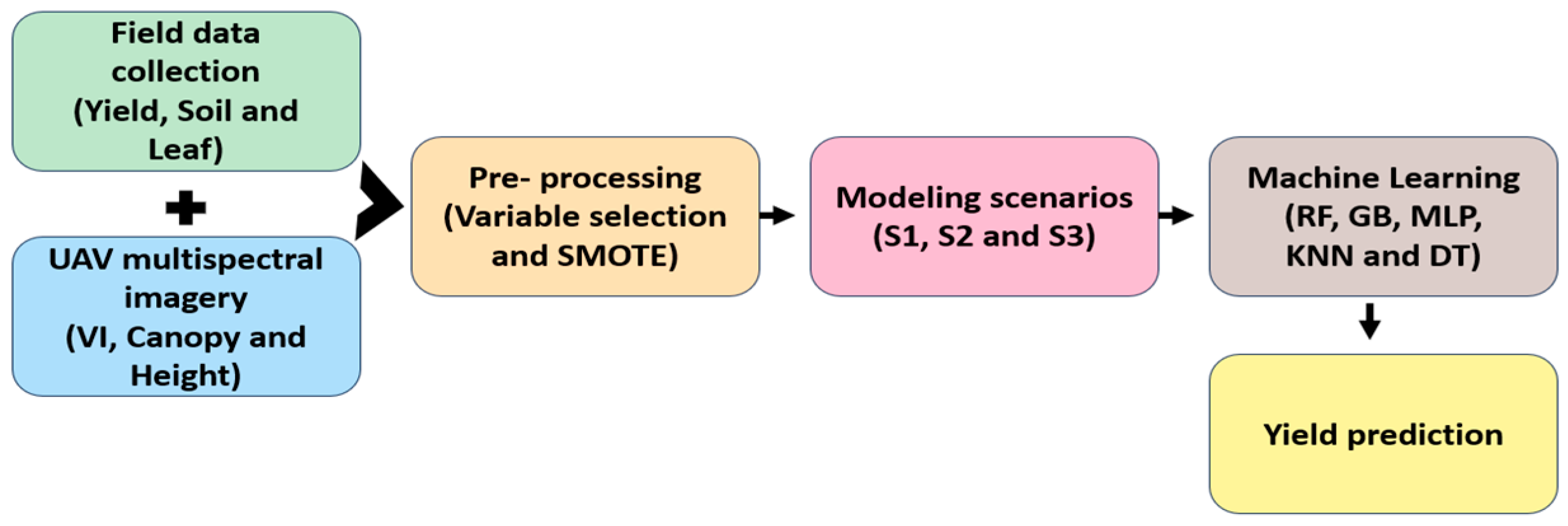
Figure 1. Methodological workflow for coffee yield prediction.
Drones 09 00717 g001
Figure 2. Location of the study area and sampling grid.
Drones 09 00717 g002
Figure 3. Yield sampling.
Drones 09 00717 g003
Figure 4. Scholander bomb.
Drones 09 00717 g004
Figure 5. Remotely piloted aircraft and multispectral sensor.
Drones 09 00717 g005
Figure 6. Example of UAV-derived imagery showing the georeferenced sampling polygon (30 cm diameter) applied to coffee plants: (a) RGB orthomosaic, (b) NDVI, (c) NDRE, and (d) EVI2.
Drones 09 00717 g006
Figure 7. Workflow of the modeling scenarios and machine learning algorithms.
Drones 09 00717 g007
Figure 8. Correlation plot for the 2020/2021 season.
Drones 09 00717 g008
Figure 9. Correlation plot for the 2021/2022 season.
Drones 09 00717 g009
Figure 10. Correlation plot for the combined seasons.
Drones 09 00717 g010
Figure 11. Actual vs. Predicted Plots for Scenarios 1 (a), 2 (b), and 3 (c).
Drones 09 00717 g011
Table 1. Summary of measured variables, classification, units, data source, and sampling period.
VariableGroupUnitData Source/MethodSampling
Period
YieldBiophysicalL plant−1Semi-mechanized harvest + volumetric methodJune 2021 and June 2022
Soil moisture (GH)Biophysical% (gravimetric)Soil sampling (0–20 cm), oven-drying methodAug. 2020, Jan. 2021, Aug. 2021, Jan. 2022
Leaf water potential (Ψw)BiophysicalMPaScholander pressure chamberSame as above
Soil fertilityBiophysical Laboratory analysis (pH, P, K, Ca, Mg, etc.)Apr. 2021 and Apr. 2022
Leaf nutrient contentBiophysicalg kg−1/mg kg−1Laboratory analysis (N, P, K, Ca, Mg, S, etc.)Jan. 2022
NDVISpectral Calculated from UAV multispectral imagesAug. 2020, Jan. 2021, Aug. 2021, Jan. 2022
NDRESpectral Same as aboveSame as above
EVI2Spectral Same as aboveSame as above
Plant heightSpectralmDSM–DTM from UAV imagesSame as above
Canopy
diameter
SpectralmManual from orthomosaic (bounding box method)Same as above
Leaf area index (LAI)Spectralm2Estimated via [28]Same as above
Table 2. Vegetation indices.
IndexEquationsReferences
NDVI (Normalized Difference Vegetation Index) N I R + R E D N I R R E D [32]
NDRE (Normalized Difference RedEdge) N I R R E D   E d g e N I R + R E D   E d g e [33]
EVI2 (Enhanced Vegetation Index 2) 2.5   N I R R E D ( N I R + 2.4 R E D + 1 ) [34]
Table 3. Dataset for machine learning.
ScenarioDependent VariableIndependent VariablesCrop Season(s)Machine
Learning
Algorithms
Scenario 1
Complete Dataset
Yield (L/plant)All collected variables:
- Soil moisture: GH_2020, GH_2021
- Leaf water potential: WP_2021, WP_2022
- Soil fertility: pH, P, K, Ca, Mg, MO, H + Al
- Leaf nutrition: N, P, K, Ca, Mg, S, Mn, Zn, B, Cu, Fe
- Spectral indices: NDVI, NDRE, EVI2
- Structural traits: plant height, canopy diameter, LAI
2020/2021
2021/2022
Combined
RF, GB, MLP, KNN, DT
Scenario 2
Selected Variables
Yield (L/plant)Only variables with highest correlation with yield:
- 2020/2021: GH_2020, GH_2021, NDRE_2020, pH
- 2021/2022: WP_2022, P_leaf, S_leaf, N_leaf, K_leaf
- Combined: NDRE_2020, GH_2021, NDVI_2020, H + Al, GH_2020
2020/2021
2021/2022
Combined
RF, GB, MLP, KNN, DT
Scenario 3
Selected Variables + SMOTE
Yield (L/plant)Same variables as in Scenario 2, with dataset expanded using SMOTE.
Tripled the number of samples from 30 to 90.
2020/2021
2021/2022
Combined
RF, GB, MLP, KNN, DT
GH: Gravimetric Humidity; WP: Water Potential; pH: Hydrogen potential; N: Nitrogen; K: Potassium; P: Phosphorus; Ca: Calcium; Mg: Magnesium; Mn: Manganese; Zn: Zinc; B: Boron; Cu: Copper; Fe: Iron; H + Al: Total acidity; SB: Sum of bases; OM: Organic matter; Prem: Remaining phosphorus; NDVI: Normalized Difference Vegetation Index; NDRE: Normalized Difference Red Edge Vegetation Index; EVI2: Enhanced Vegetation Index 2; LAI: Leaf Area Index.
Table 4. Descriptive statistics of yield for the 2020/2021 and 2021/2022 crop seasons.
Statistic Yield 2020/2021Yield 2021/2022
Mean10.205.47
Min–Max1.00–22.000.00–22.00
Standard deviation4.795.25
Skewness 0.431.12
Variation coefficient (%) 46.9696.15
Table 5. RMSE and MAPE metrics for the 2020/2021, 2021/2022, and combined crop seasons (2020/2021 and 2021/2022), considering the original database (all variables).
Original Dataset
ModelsSeason 2020/2021Season 2021/2022Combined Crop Season
(2020/2021 + 2021/2022)
TrainingTestTrainingTestTrainingTest
RMSEMAPERMSEMAPERMSEMAPERMSEMAPERMSEMAPERMSEMAPE
RF4.47 ± 3.62-6.543.388.02 ± 8.124.50 ±6.118.59-5.54 ± 5.60-11.110.98
GB4.72 ± 3.72-9.864.028.81 ± 9.274.74 ± 9.6113.66-5.35 ± 5.75-11.231.15
MLP5.71 ± 4.06-5.543.119.35 ± 10.623.97 ± 4.9510.46-6.42 ± 5.70-12.411.53
KNN4.45 ± 3.87-4.212.516.71 ± 8.602.27 ± 2.5912.19-6.38 ± 5.94-11.801.13
DT4.96 ± 3.87-13.066.1610.30 ± 10.776.41 ± 15.5715.41-6.58 ± 7.38-13.351.71
Table 6. RMSE and MAPE metrics for the 2020/2021, 2021/2022, and combined crop seasons (2020/2021 and 2021/2022), considering only the variables selected based on their correlations with yield for each season.
Dataset with Selected Variables (Variables with the Highest Correlations with Yield)
ModelsSeason 2020/2021
(GH_2020, GH_2021, pH and NDRE)
Season 2021/2022
(N, S, P, K Leaf and WP_2022)
Combined (2020/2021 + 2021/2022)
(H + Al, NDRE_2020, GH_2020, GH, 2021 and NDVI_2020)
TrainingTestTrainingTestTrainingTest
RMSEMAPERMSEMAPERMSEMAPERMSEMAPERMSEMAPERMSEMAPE
RF5.01 ± 3.73-2.611.436.92 ± 7.89-9.68-6.97 ± 7.65-5.263.27
GB5.73 ± 3.99-2.660.897.52 ± 9.57-9.14-7.97 ± 8.86-5.532.48
MLP4.72 ± 3.52-1.780.7411.92 ± 13.45-15.58-8.06 ± 6.91-5.341.80
KNN4.51 ± 3.00-2.761.556.77 ± 7.95-11.18-6.30 ± 6.70-5.262.26
DT6.20 ± 4.92-3.020.668.34 ± 8.12-15.92-8.41 ± 9.41-10.883.79
Table 7. RMSE and MAPE metrics for the 2020/2021, 2021/2022, and combined crop seasons (2020/2021 and 2021/2022), considering only the variables selected based on their correlations with yield and using the SMOTE technique to triple the dataset size.
Dataset with Selected Variables Using the SMOTE Technique (Tripling the Data Volume)
ModelsSeason 2020/2021
(GH_2020, GH_2021, pH and NDRE)
Season 2021/2022
(N, S, P, K Leaf and WP_2022)
Combined (2020/2021 + 2021/2022)
(H + Al, NDRE_2020, GH_2020, GH, 2021 and NDVI_2020)
TrainingTestTrainingTestTrainingTest
RMSEMAPERMSEMAPERMSEMAPERMSEMAPERMSEMAPERMSEMAPE
RF1.39 ± 2.31-2.090.831.75 ± 2.29-9.04-2.69 ± 4.63-6.894.41
GB1.24 ± 2.49-2.280.880.91 ± 1.99-12.42-2.56 ± 4.64-7.844.24
MLP1.72 ± 2.41-2.821.772.29 ± 2.11-13.11-3.34 ± 4.06-5.612.26
KNN1.74 ± 2.23-5.142.903.15 ± 4.12-17.64-3.32 ± 4.97-5.492.88
DT0.90 ± 2.67-3.140.671.06 ± 3.86-10.53-2.15 ± 5.98-11.316.37
Table 8. Significant pairwise differences (p < 0.05) in RMSE among algorithms, separated into within-season and cross-season comparisons.
ScenarioSeasonType of ComparisonSignificant Differences
(p < 0.05)
32020/2021Within-season
-
DT × MLP; DT × KNN
32021/2022Within-season
-
RF × GB; RF × KNN
-
GB × MLP; GB × KNN
-
MLP × DT
-
KNN × DT
3CombinedWithin-season
-
MLP × RF
-
DT × MLP; DT × KNN
12020/2021 ×
2021/200
Cross-season
-
RF × GB; RF × MLP
12021/2022 × CombinedCross-season
-
MLP × GB
22020/2021 × CombinedCross-season
-
KNN × MLP
22021/2022 × CombinedCross-season
-
MLP × KNN
32020/2021 × 2021/2022Cross-season
-
RF × MLP; RF × KNN
-
GB × MLP; GB × KNN
-
MLP × KNN
-
DT × RF; DT × MLP; DT × KNN
32020/2021 × CombinedCross-season
-
RF × GB; RF × MLP;
-
RF × KNN
-
GB × MLP; GB × KNN
-
MLP × KNN
-
DT × RF; DT × GB; DT × MLP; DT × KNN; DT × RF
32021/2022 × CombinedCross-season
-
RF × MLP; RF × KNN
-
GB × RF; GB × MLP; GB × KNN; GB × DT
-
DT × RF; DT × MLP; DT × KNN
Disclaimer/Publisher’s Note: The statements, opinions and data contained in all publications are solely those of the individual author(s) and contributor(s) and not of MDPI and/or the editor(s). MDPI and/or the editor(s) disclaim responsibility for any injury to people or property resulting from any ideas, methods, instructions or products referred to in the content.