Risk-Aware UAV Trajectory Optimization Using Open Urban GIS Data and Target Level of Safety Constraints

Abstract

Integrating Unmanned Aerial Vehicles (UAVs) into urban airspace requires a risk-aware approach to strategic flight planning and trajectory optimization, particularly for beyond-visual-line-of-sight operations. Existing regulatory frameworks impose strict restrictions and lack dynamic, trajectory-based risk assessments. This study presents a methodology to compute efficient UAV flight paths that comply with a predefined Target Level of Safety (TLS) for ground risk. An A* algorithm with an adaptive, risk-weighted cost function optimizes trajectories by balancing flight efficiency and ground risk exposure. The risk model incorporates key urban factors, including population exposure, road-traffic density and flow, sheltering effects, UAV-specific parameters, and wind conditions. The approach is validated through a large-scale simulation study using synthetic urban environments, systematically analyzing TLS compliance and the impact of UAV parameters on optimal trajectories. In a real-world case study using open urban GIS data, the method achieved a 72.2% reduction in induced ground risk compared to the direct path, while increasing the detour factor only to $1.06$ and maintaining full TLS compliance, demonstrating its practical relevance for strategic, risk-aware UAV flight planning.

1. Introduction

With the emergence of Uncrewed Aerial Vehicle (UAV)—in particular electric Vertical Take-off and Landing (eVTOL) systems suited for space-constrained urban operations—new users are entering the airspace. These vehicles enable new modes of operation but also raise safety concerns regarding both ground and air risks. Authorities have responded by establishing UAV geographical zones [1], which restrict or prohibit operations. These zones address various interests, such as minimizing air risk near aerodromes, mitigating ground risk by avoiding roads and rail corridors, reducing noise over nature reserves, or protecting privacy in residential areas (Figure 1).

Within the current regulatory framework, flights entering a geographical zone must operate in the specific category, requiring individual authorisation [1]. Risk assessments are typically conducted using the Specific Operations Risk Assessment (SORA) methodology [2], which provides a structured framework but assumes ground risk to be uniformly distributed over large areas, does not cover all combinations of operational scenarios, and requires a separate assessment for each mission. While pragmatic and accessible to non-safety specialists, it is resource-intensive, slow, and poorly adaptive to changing conditions. These constraints highlight the need for a more agile, data-driven approach to risk assessment, where optimization methods can explicitly balance efficiency and safety objectives under predefined Target Level of Safety (TLS) requirements, enabling the computation of mission-specific UAV trajectories that would not be achievable with static approaches.

In this study, we present a methodology for strategic pre-flight planning to derive energy-efficient flight paths for small UAV while ensuring compliance with a predefined TLS for ground risk, in line with the International Civil Aviation Organization (ICAO) concept of maintaining risk at or below acceptable thresholds [3]. Building on our previous work [4], the method determines optimal trajectories for a given UAV configuration, considering the probability of uncontrolled descent from safety-critical events. Directional ground risk maps are generated, integrating event probability, spatial risk distribution, ballistic descent dynamics, wind effects, and sheltering from buildings or vegetation. Then, an A* search with an adaptive, risk-weighted cost function finds the shortest feasible trajectory while keeping the cumulative ground risk below the specified TLS. The method is validated in large-scale simulations and applied to a real-world scenario using open urban Geographic Information System (GIS) data to demonstrate practical relevance.

This paper continues with a review of the state of the art, focusing on safety assessment, risk modeling, and optimal pathfinding for UAV. Section 4 introduces our risk assessment methodology, which evaluates ground risk and develops directional maps that encode both the magnitude and directionality of risk, enabling routes to account for anisotropic patterns such as crowd flows or infrastructure layout. Subsequently, Section 5 presents the pathfinding algorithm, which computes energy-optimal flight paths on these directional risk maps while ensuring compliance with a specified TLS for ground risk. Section 6 describes the simulation setup, the real-world data used for validation, and the UAV parameters considered in the study. The results are presented and discussed in Section 7. Finally, Section 8 discusses potential extensions and future integration of additional factors and data sources.

2. State of the Art

2.1. Regulatory Background in Aviation

Regulation (EU) 2019/947 [1] governs the safe operation of UAV in the European Union. It establishes risk mitigation measures for both the air risk for crewed air traffic and the Ground Risk Buffer (GRB) to protect third parties on the surface. For operations in the specific category, three options for risk mitigation are proposed. Firstly, two Standard Scenarios (STS) are available, describing predefined operations, one each for Visual Line of Sight (VLOS) and Beyond Visual Line of Sight (BVLOS), which require ground observers to ensure the absence of uninvolved persons on the ground (i.e., controlled ground). Secondly, a Predefined Risk Assessment (PDRA) is an Acceptable Means of Compliance (AMC). Each PDRA is a specific scenario with an already conducted risk assessment. However, all published PDRA are limited to controlled ground or sparsely populated areas. Thirdly, the SORA methodology in its current Edition 2.0 [2,5] represents an authorisation-oriented, operation-centric risk assessment. A planned update, Edition 2.5 [6], has been released for consultation and is expected to become binding under EASA regulations in the near term. SORA determines the Intrinsic Ground Risk Class (iGRC) and Air Risk Class (ARC), maps the outcome to a Specific Assurance Integrity Level (SAIL), and derives Operational Safety Objectives (OSOs) via a checklist- and criterion-based process. The assessment relies on scenario-level assumptions and area-averaged population exposure; recommended datasets typically have coarse spatial resolution, so local heterogeneity and time-dependent exposure are not explicitly represented. SORA evaluates a defined concept of operation (including intended airspace volumes or reference routes) for admissibility and required mitigations; it does not compute trajectories nor optimize path choices. For BVLOS flights over populated areas, SORA often leads to high (or undefined) SAIL levels that are challenging to mitigate with currently accepted measures, and such operations remain subject to strict restrictions.

In conventional aviation, an alternative concept–the acceptable level of safety–has been applied for decades, expressed via the TLS as the maximum tolerable accident rate [3]. A commonly used value is 1 × 10⁻⁷ fatal accidents per flight [7], although ambitious targets such as SESAR’s objective of achieving a tenfold safety improvement are under discussion [7]. The TLS is not applied homogeneously throughout the flight but has been adapted to various applications [8], such as specific phases of flight (e.g., landing, take-off, oceanic crossing) or operational hours (e.g., surface movements). Compliance with the TLS is typically demonstrated through extensive quantitative risk assessments and validated by regulators. It has also been suggested to transfer this concept to Uncrewed Aerial System (UAS) operations [9]. In contrast to manned aviation, however, a UAV accident does not necessarily imply fatal consequences. This study, therefore, explores the application of TLS to UAV trajectory optimization under explicit consideration of ground risk.

2.2. Quantification of Ground Risk

In SORA, the iGRC is assigned through discrete classes based on the maximum UAV characteristic dimensions and speed, together with area-wide population density [2,6]. These scales, derived from reference scenarios by JARUS, enable a standardized authorisation process but abstract from detailed modeling, as they assume static densities and neglect local or temporal variations. For scientific risk assessment, however, severity and likelihood need to be modeled explicitly, as adopted in this study. Risk assessment for UAS requires quantifying the severity and the likelihood of accidents. For ground risk, potential severity is determined by the kinetic energy at impact, which can be fatal even for small UAV at sufficiently high velocities, particularly when persons are in an unprotected posture [10,11]. It depends on parameters such as UAV mass, altitude, size, and descent velocity, and has been related to injury probability through biomechanical impact models that account for posture and exposure [12,13,14,15]. Likelihood, in contrast, is governed by the probability of human presence at the potential impact site, influenced by factors such as population density, mobility patterns [16,17,18] and the platform-specific failure probability [19,20,21].

Accident modeling for multirotor systems frequently assumes a ballistic descent, leading to impact points close to the failure location [22,23,24]. Further improvements incorporate wind effects and positional uncertainty, producing probability density functions for impact footprints [25]. Aerodynamic effects have also been considered: the drag coefficient varies substantially with pitch angle, significantly affecting terminal velocity and impact energy on steeper pitches [26]. Partial-failure scenarios, such as the loss of one or more propulsion units, have been shown to alter the location and velocity of impact [27].

The probability of casualties is commonly obtained by coupling these crash models with spatial exposure data. Early approaches relied on static population-density maps derived from different data sets [16,28], while more recent studies have incorporated spatiotemporal datasets from mobile-phone location records, road-traffic sensors, or activity-based modeling [21,29,30]. Many authors also account for sheltering effects–reductions in fatality probability due to the presence of buildings, vegetation, or vehicles–by applying location-specific coefficients [24,31]. Such data are frequently obtained from open geospatial sources like Open Street Map (OSM) to identify streets, buildings, and urban areas [4,32].

2.3. Sheltering Effects

Sheltering effects refer to infrastructure or vegetation mitigating the risk of uncontrolled UAV descents. Buildings, trees, and vehicles are examples of features contributing to these effects [21,31]. One approach incorporates the sheltering effect in the fatality likelihood, e.g., based on the resulting kinetic energy and the population density [9]. More recent studies refine this method through geospatial analysis, estimating the protection offered by specific objects, from minimal protection over lakes to substantial safety gains near reinforced buildings [33].

Instead of embedding sheltering into a composite likelihood function–which inherently mixes terminal kinetic energy, exposure probability, and fatality probability, and thereby reduces transparency–an alternative is to treat sheltering as a physical process that dissipates impact energy before injury modeling. In this energy-absorption approach, the kinetic impact energy is first reduced according to material-specific absorption properties, and the residual energy is then used to estimate fatality probability. Kim and Bae [31] proposed a simplified variant with a binary reduction factor, assuming 100% protection indoors and 0% outdoors, including inside vehicles. In practice, however, intermediate values are common and highly context-dependent. For example, a small or slow UAV may be completely stopped by a tree, while a heavier, faster vehicle loses only a fraction of its energy. Material-specific data provide a more differentiated picture: laminated glass requires approximately 450 J to penetrate [34], reinforced concrete can absorb up to 13,558 J, automobile steel around 271 J, and wooden joists about 68 J [35].

This explicit separation of exposure, energy dissipation, and injury probability offers two advantages over the embedded-likelihood method: it makes the modelling assumptions transparent and allows direct substitution of material properties when more accurate or location-specific data are available. It also facilitates the extension of the model to dynamic exposure scenarios, such as diurnal variations in pedestrian and vehicle densities [36,37]. For example, while experimental studies show that laminated windshields can remain intact under impacts from small UAV [38], the visual obstruction they cause still presents a safety hazard. In contrast, large UAV with impact energies comparable to a human head impact at 16 m/s⁻¹ (approx. 614 J) have been shown to penetrate windshields, posing a severe risk of injury or fatality [39].

2.4. Risk-Based Optimal Pathfinding

For pathfinding, three common approaches are graph-based shortest path search algorithms [4,40], optimal control [41], genetic algorithms [42], and on-board obstacle avoidance supported by machine learning [43]. Optimal control is well suited to the continuous dynamics of complex trajectories but often suffers from numerical approximation errors and high computational cost, which can lead to suboptimal solutions under real-time constraints. Graph-based methods such as A* avoid these issues, offering efficient search with guaranteed optimality [44,45]. Recent refinements adapt A* to mission-specific needs: Braßel et al. [4] use A* to evaluate UAS hangar positions in complex environments, Du [46] combine A* with cooperative task allocation for multi-UAV search-and-rescue, and Xu et al. [47] introduce an adaptive neighborhood A* that minimizes inflection points, creating smoother and more efficient 3D trajectories. These developments show that A* can be adapted to operational constraints while remaining efficient, making it suitable for use with risk-based cost layers from ground-risk maps. However, dynamic cost weighting or the use of heuristics that are not admissible or monotone can break A*’s consistency, removing its guarantee of finding a globally optimal solution.

Ground-risk maps provide georeferenced information layers that quantify spatial risk and are therefore well suited as cost functions in pathfinding [48,49]. These maps integrate crash dynamics, exposure probabilities, and, in more advanced models, sheltering effects to reflect the spatial distribution of risk for a given operational area [24,50]. Some pathfinding strategies [51] use impact-probability radii to steer trajectories away from high-density areas, but often omit mitigating factors such as sheltering. More recent work addresses this by explicitly incorporating risk-based metrics into path optimization [37,48,49,52,53], or by constraining flights to pre-assessed corridors whose width varies according to the underlying ground risk [31].

Enhancements to ground-risk maps have included dynamic population models, which update exposure estimates in real time based on activity patterns [21]. Extending the concept further, Gao et al. [54] proposed 3D virtual safety risk terrains, embedding crash-dynamics models, sheltering coefficients, and exposure into volumetric exclusion zones.

3. Observed Limitations and Contributions

Despite substantial prior work on ground-risk assessment for UAV operations, important gaps remain. From a regulatory perspective, SORA (cf. Section 2.1) is an authorisation tool that evaluates a defined concept of operation; it neither computes nor optimizes trajectories. Ground risk is handled via area-averaged exposure with coarse spatial resolution and without time dependence, so local heterogeneity along a concrete route is not captured. In the literature, planning approaches either optimize single objectives (e.g., minimum-risk routing) or preselect distance-optimal paths and post-assess risk, rather than solving a multi-objective trade-off during search. Exposure is frequently treated uniformly, overlooking both the distinction between risk to pedestrians and to occupants of road vehicles and time–location dependence (e.g., diurnal road-traffic patterns). Explicit TLS constraints are rarely enforced, endurance limits are often ignored, and risk fields are commonly isotropic or static, lacking descent dynamics, wind drift, and sheltering effects. Together, these limitations impede mission-specific, TLS-compliant trajectory planning in urban settings.

This work addresses the above limitations by integrating trajectory optimization and ground-risk evaluation into a single framework:

• We treat a predefined TLS as a hard constraint on accumulated, directional ground risk and jointly consider endurance, yielding mission-specific, TLS-compliant trajectories.
• We construct per-cell, directional risk maps from open urban GIS, accounting for ballistic descent, wind drift, and sheltering, and model spatiotemporal exposure that distinguishes pedestrians from vehicle occupants.
• We employ an A* search with adaptive weighting that balances flight time and risk, including distance normalization via a detour factor and dynamic weight adaptation.
• We validate on synthetic and real urban maps, reporting TLS compliance and detour factors to quantify the efficiency–safety trade-off.

4. Risk Assessment Methodology

4.1. Structure and Workflow

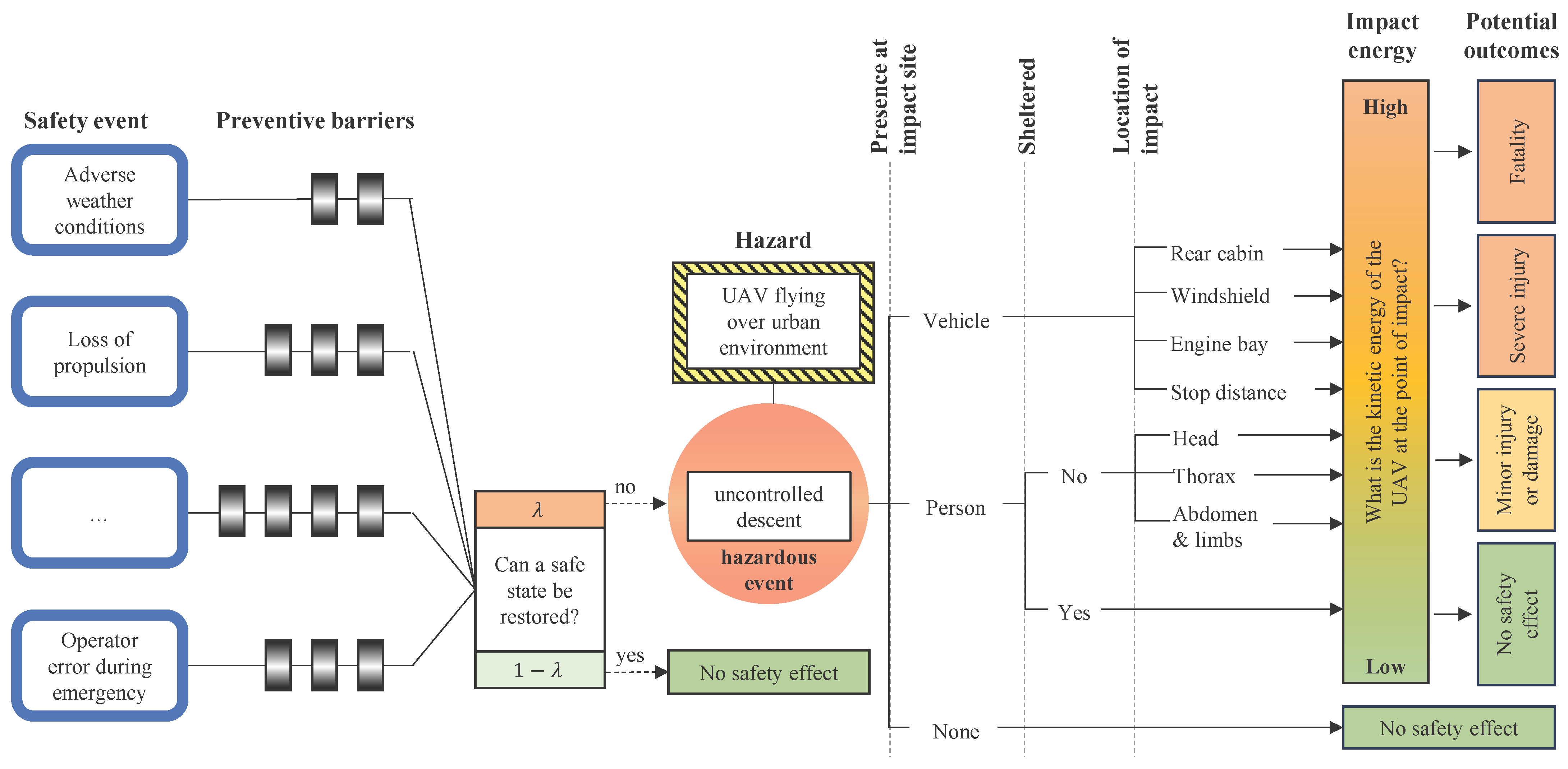
To overcome the limitations outlined in Section 3, we propose a methodology for mission-specific, time-dependent ground-risk assessment and its integration into multi-objective UAV path planning under a specified TLS. Our approach focuses on the event tree segment of the bow-tie model in Figure 2, which evaluates the consequences following a hazardous event. The input to this process is the overall probability of an uncontrolled descent, representing the combined likelihood of all relevant safety events: technical, operational, environmental, and human factors. Using geographic data for the target area, we assess the resulting ground risk for each possible impact location. This ground risk is then incorporated as a cost layer in the pathfinding algorithm, allowing the computed trajectory to account for distance and risk.

This study focuses on individual fatality risk, i.e., the probability of a fatal injury to a single third party–either a pedestrian or an occupant of a vehicle–resulting from an uncontrolled descent, as the small UAV considered is unlikely to cause multiple fatalities.

The sequence of risk assessment comprises three main stages:

• Severity assessment: The potential outcome of an uncontrolled descent is quantified based on UAV parameters, flight altitude, and local conditions at the impact site. These include the sheltering effect of surrounding structures or vegetation, as well as the characteristics of the impacted target. For pedestrians, severity varies with the body region struck [11]; for vehicles, it depends on impact location (e.g., windshield, roof, engine bay) and vehicle speed.
• Likelihood assessment: The conditional probability of an impact is given by the joint occurrence of (i) a person or vehicle being present in the potential impact area, and (ii) an uncontrolled descent, based on the cumulative failure probability of all relevant safety events (platform-specific) and the dwell time above the cell. The likely drift path of the falling UAV–determined by ballistic descent dynamics and wind direction–is taken into account, resulting in anisotropic likelihood values.
• Risk estimation: The ground risk is computed as the product of severity and likelihood, yielding the directional fatality risk value assigned to the corresponding edge of the motion graph.

These elements require georeferenced information on exposure likelihood and sheltering features, from which we derive time-dependent and platform-specific ground risk maps. Following the aviation concepts of contingency areas and protected volumes [55], the maps are inflated via Gaussian convolution parameterized by the expected Total System Error, providing safety margins for navigation errors, control delays, and wind drift during normal operation. The resulting maps serve as cost layers in a multi-objective pathfinding algorithm that minimizes flight energy while ensuring compliance with the specified TLS under varying environmental, temporal, and mission conditions.

4.2. UAV Impact Energy

For severity assessment, the UAV’s impact energy must be estimated. Ballistic descent dynamics are influenced by factors such as initial velocity, partial rotor or control functionality, and the vehicle’s attitude (yaw, pitch, and roll) [26]. In this study, a worst-case scenario is assumed: an instantaneous, complete loss of all lift-generating devices, leading to a ballistic descent in still air with quadratic aerodynamic drag and no residual lift from rotors or parachutes, thereby producing the maximum possible impact energy (‘free fall’).

Assuming a uniform gravitational field and air resistance proportional to the square of the fall velocity, the net vertical force acting on the UAV is the difference between its weight W, which pulls the UAV downward, and the aerodynamic drag force D, which resists the motion and grows stronger at higher velocities. From Newton’s second law of motion, the vertical acceleration for the free fall ${\displaystyle \frac{\mathrm{d}{v}_{\mathrm{fall}}}{\mathrm{d}t}}$ can be expressed as:

$$\frac{\mathrm{d}{v}_{\mathrm{fall}}}{\mathrm{d}t}·m_{\mathrm{UAV}}=W-D$$

(1)

where the gravitational force W and the aerodynamic drag force D are given by:

$$\begin{array}{cc}\hfill W& =m_{\mathrm{UAV}}g\hfill \end{array}$$

(2)

$$\begin{array}{cc}\hfill D& ={\displaystyle \frac{1}{2}}\rho C_d{A}_{\mathrm{UAV}}{v}_{\mathrm{fall}}^2\hfill \end{array}$$

(3)

Here, $m_{\mathrm{UAV}}$ is the UAV mass, $g=9.81 \mathrm{m}/{\mathrm{s}}^{-2}$ is the gravitational acceleration, $\rho =1.225 \mathrm{k}\mathrm{g}/{\mathrm{m}}^{-3}$ is the air density at sea level, $C_d$ is the drag coefficient, $A_{\mathrm{UAV}}$ is the UAV reference area, and $v_{\mathrm{fall}}$ is the vertical fall velocity.

Inserting the previous equations into Equation (1) yields the ordinary differential equation for the fall:

$$\frac{\mathrm{d}{v}_{\mathrm{fall}}}{\mathrm{d}t}=g-{\displaystyle \frac{1}{2·m_{\mathrm{UAV}}}}·\rho ·c_D·S_{\mathrm{UAV}}·v_{\mathrm{fall}}^2$$

(4)

We employ the explicit Runge–Kutta method [56] of order 4(5) to numerically integrate Equation (4) over time t until the UAV reaches the ground. The resulting descent duration is denoted as $t_{\mathrm{fall}}$, representing the time from the onset of free fall to impact. The integration starts from the effective fall height

$$h_{\mathrm{fall}}=h_{\mathrm{AGL}}-h_{\mathrm{obstacle}}$$

(5)

where $h_{\mathrm{AGL}}$ is the UAV altitude above the local ground level, and $h_{\mathrm{obstacle}}$ is the height of the highest elevated structures at the impact location (e.g., buildings, vegetation, or other structures). From this height, $v_{\mathrm{fall}}\left(t\right)$ is integrated over t until the altitude relative to the local ground level reaches zero, using cumulative trapezoidal numerical integration to obtain the vertical impact velocity $v_{\mathrm{impact}}$. The kinetic energy $E_{\mathrm{kin}}$ is then computed as

$$E_{\mathrm{kin}}={\displaystyle \frac{1}{2}}{m}_{\mathrm{UAV}}·v_{\mathrm{impact}}^2.$$

(6)

In our study, sheltering captures the mitigating effect of obstacles that absorb a portion of the UAV’s kinetic energy, thereby reducing the impact force. The total energy transferred to a target is expressed as the terminal energy $E_{\mathrm{term}}$ by reducing $E_{\mathrm{kin}}$ with the energy absorption $E_{\mathrm{absorb}}$ of the sheltering object:

$$E_{\mathrm{term}}=max\left(E_{\mathrm{kin}}-E_{\mathrm{absorb}},0\right)$$

(7)

This formulation focuses on measurable energy reduction rather than directly estimating fatality probabilities [9,21]. By separating sheltering effects from the subsequent fatality probability calculation, we can employ a standardized risk map without recalculating individual fatality functions for each grid cell, which significantly accelerates the pathfinding. Moreover, $E_{\mathrm{absorb}}$ integrates seamlessly into current regulatory frameworks, where kinetic energy is a key safety metric [1].

4.3. Modeling of Pedestrian Fatality Risk

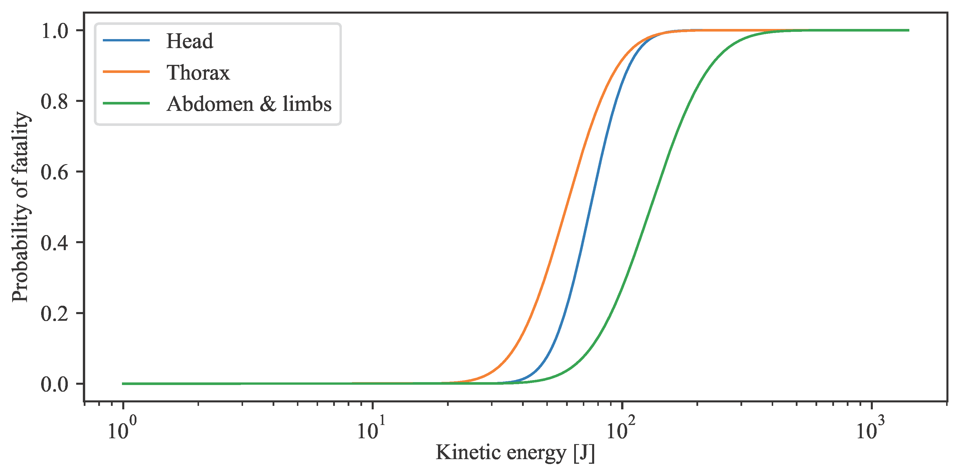
Assuming the presence of a person at the impact location, the potential for a fatal injury caused by the terminal energy $E_{\mathrm{term}}$ from Equation (7) must be quantified. Following Range Safety Group [11], who investigated the probability of fatality from debris impacts for different body regions (head, thorax, abdomen, limbs) and poses (standing, seated, prone), we assumed a log-normal model for the fatality probability $P_i$ when body part i is struck. Thus, $P_i$ for a given $E_{\mathrm{term}}$ is computed using the cumulative density function with location parameter ${\alpha }_i$ and shape parameter ${\beta }_i$:

$$P_i\left(E_{\mathrm{term}}\mid {\alpha }_i,{\beta }_i\right)={\displaystyle \frac{1}{2}}·\left(1+erf\left({\displaystyle \frac{ln{E}_{\mathrm{term}}-ln{\alpha }_i}{\sqrt{2}·{\beta }_i}}\right)\right)$$

(8)

where $erf\left(·\right)$ is the error function.

Using Equation (8) and the parameters from

Table 1. Parameters for pedestrian fatalities assuming a standing person [11].

Body Part	Area ${\mathit{A}}_{\mathbf{person},\mathbf{i}}$	Relative Area	Log-Normal Distribution
	[m2]	${\mathit{\sigma }}_{\mathit{i}}$  [%]	${\mathit{\alpha }}_{\mathit{i}}$  [J]	${\mathit{\beta }}_{\mathit{i}}$
Head	0.025	29.27	74.57	0.2802
Thorax	0.038	43.21	59.66	0.3737
Abdomen, limbs	0.0242	27.52	130.16	0.4335

, the resulting probability of fatality per body part is visualized depending on $E_{\mathrm{term}}$ in Figure 3.

The total fatal probability for a person $F_{\mathrm{person}}$ depends on the percentage of the exposed area per body part ${\sigma }_i$. As we focus on pedestrians, we assume all persons are standing with the value in Table 1 [11], while acknowledging that local distributions of standing, seated, or prone individuals could provide valuable input for future applications and should be addressed in sensitivity analyses.

$$F_{\mathrm{person}}\left(E_{\mathrm{term}}\mid {\alpha }_i,{\beta }_i\right)=\sum _{i=1}^n{\sigma }_i·P_i\left(E_{\mathrm{term}}\mid {\alpha }_i,{\beta }_i\right)$$

(9)

The resulting $F_{\mathrm{person}}$ is the probability of a crashing UAV to injure a person fatally. For the likelihood of such fatalities, the probability of a person being present at the impact location must be modeled. This probability varies spatially and temporally, for example, with rush-hour traffic, weekend shopping crowds, or events in stadiums. Ideally, presence data are available and integrated into the UAV path planning process. Possible sources include mobile network usage, road traffic, and pedestrian counts, points of interest combined with population statistics, and live sensor feeds. The fatality risk for a pedestrian in a cell $R_{\mathrm{person}}$, in the event of an uncontrolled UAV crash, is obtained by summing over all body parts i, combining the fatality probability $F_i$ (Equation (9)) with the probability of presence in the UAV footprint:

$$R_{\mathrm{person}}=\sum _i{F}_i·{\displaystyle \frac{A_{\mathrm{UAV}}·A_{\mathrm{person},i}}{{\delta }_{\mathrm{cell}}^2}}·d_{\mathrm{cell}}$$

(10)

Here, $A_{\mathrm{UAV}}$ is the projected UAV footprint on the ground [${\mathrm{m}}^2$], $A_{\mathrm{Person},i}$ is the projected area of body part i [${\mathrm{m}}^2$] as given in Table 1, ${\delta }_{\mathrm{cell}}$ the cell resolution of the risk map [$\mathrm{m}$], and $d_{\mathrm{cell}}$ the estimated person density in the cell [persons/${\mathrm{m}}^2$].

4.4. Modeling of Street Fatality Risk

The street–risk model is developed for a passenger car as the reference case; other vehicle types can be handled analogously by adapting the zone geometry and parameters.

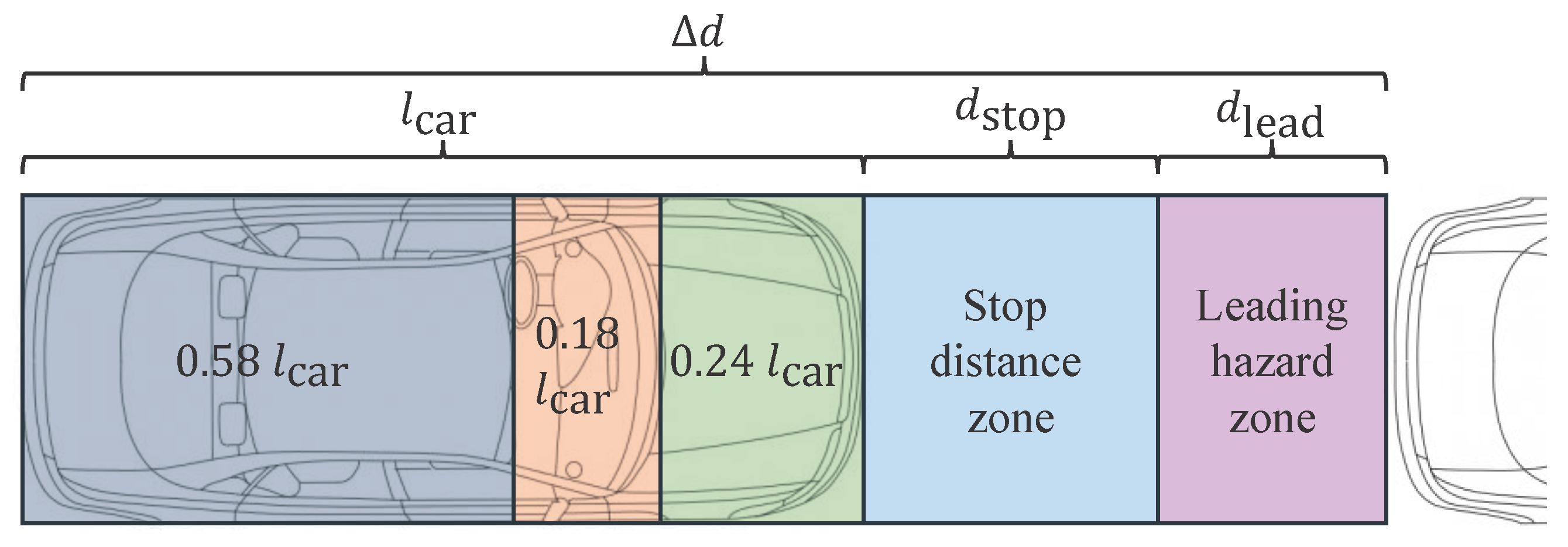
For passenger cars, hazard zones are defined as shown in Figure 4. An uncontrolled UAV descent may result in an impact on a road segment that is unoccupied at the time of impact (leading hazard zone), within the driver’s braking distance (stop distance zone), or directly on the vehicle (vehicle zone). In the latter case, the impact location is further subdivided into the engine bay (green), windshield (red), and rear cabin (blue).

The driver’s fatality risk depends on the impact zone, the vehicle’s speed, and $E_{\mathrm{term}}$ Equation (7), which may increase or decrease the risk compared to a pedestrian. The vehicle speed is assumed to equal the road speed limit $v_{\mathrm{car}}$, yielding the worst-case impact energy. The average spacing between two vehicles $\Delta d$ is then computed from the street flow rate q as

$$\Delta d={\displaystyle \frac{v_{\mathrm{car}}}{q}}$$

(11)

Here, q depends on multiple factors, such as street type, seasonality, and diurnal variation. Different data sources may be used, ranging from peak-hour assumptions to historical records or live road-traffic data.

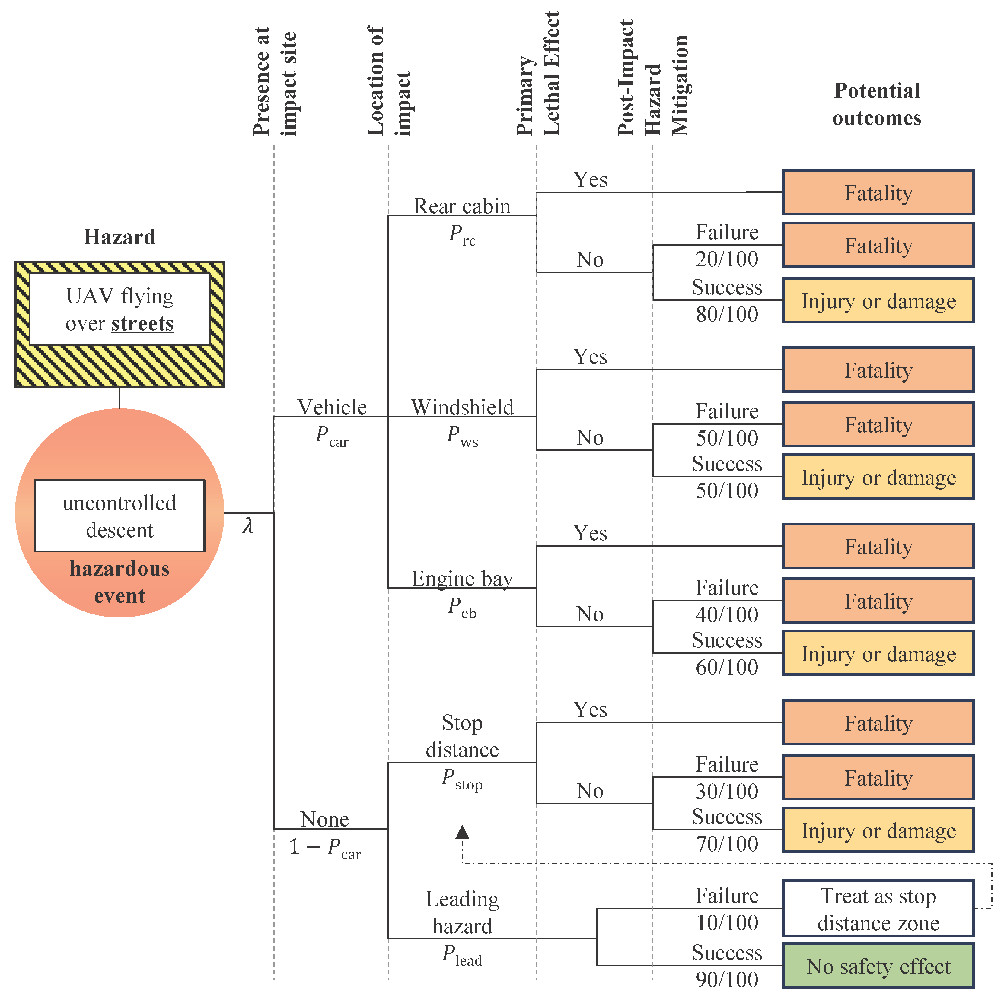
The event tree in Figure 5 evaluates outcomes of an uncontrolled UAV descent over a street. The UAV may collide with a vehicle or, if no vehicle is present, crash into the stop distance zone of a car or leading hazard zone (Figure 4). Each scenario has a probability of fatal consequences. A direct vehicle impact may cause immediate fatalities. The driver’s reaction determines the risk of secondary accidents. Startled reactions may lead to loss of control, with assumed fatality probabilities between 10/100 and 80/100. These estimates require further validation through human factor studies. The following section derives impact probabilities for each hazard zone.

4.4.1. Leading Hazard Zone

If the UAV impacts the leading hazard zone, sufficient distance is left to stop the vehicle before arriving at the impact location. However, the UAV may be too small for the driver to see it in time. We assume a detection probability $P_{\mathrm{detect}}=0.9$ for the driver to see, react, and avoid the UAV. For the $1-P_{\mathrm{detect}}$ cases, the driver does not detect the UAV soon enough and is considered inside the stop distance zone.

Figure 5. Event-tree for an uncontrolled UAV descent over a street, depending on impact location with primary and secondary effects.

Figure 5. Event-tree for an uncontrolled UAV descent over a street, depending on impact location with primary and secondary effects.

4.4.2. Stop Distance Zone

When a UAV impacts within the stop distance zone of a car, it loses its kinetic energy upon impact with the ground. However, the vehicle collides with the debris, leading to potential secondary effects. The stop distance $d_{\mathrm{stop}}$ is computed from the maximum road speed $v_{max}$, the driver reaction time $t_{\mathrm{r}}=1 \mathrm{s}$ and vehicle deceleration $a_{\mathrm{car}}=7.5 {\mathrm{m}/\mathrm{s}}^{-1}$ with:

$$d_{\mathrm{stop}}=v_{\mathrm{car}}·t_{\mathrm{r}}+{\displaystyle \frac{{v_{\mathrm{car}}}^2}{2·a_{\mathrm{car}}}}$$

(12)

During braking, the velocity decreases over time:

$$v_{\mathrm{car}}\left(t\right)=v_{max}-a_{\mathrm{car}}t,0\le t\le {\displaystyle \frac{v_{max}}{a_{\mathrm{car}}}}$$

(13)

The vehicle undergoes an inelastic collision with the UAV debris, where the post-impact velocity $v_{\mathrm{inel}}$ follows from momentum conservation:

$$v_{\mathrm{inel}}\left(t\right)={\displaystyle \frac{m_{\mathrm{car}}{v}_{\mathrm{car}}\left(t\right)+m_{\mathrm{UAV}}{v}_{\mathrm{UAV}}}{m_{\mathrm{car}}+m_{\mathrm{UAV}}}}$$

(14)

For the considered case, the UAV debris is stationary upon impact, i.e., $v_{\mathrm{UAV}}=0$, which simplifies the equation to:

$$v_{\mathrm{inel}}\left(t\right)={\displaystyle \frac{m_{\mathrm{car}}{v}_{\mathrm{car}}\left(t\right)}{m_{\mathrm{car}}+m_{\mathrm{UAV}}}}$$

(15)

with $m_{\mathrm{car}}$ as the vehicle mass and $m_{\mathrm{UAV}}$ as the UAV mass. The kinetic-energy loss from the impact is

$$E_{\mathrm{loss}}\left(t\right)={\displaystyle \frac{1}{2}}{m}_{\mathrm{car}}{v}_{\mathrm{car}}{\left(t\right)}^2-{\displaystyle \frac{1}{2}}\left(m_{\mathrm{car}}+m_{\mathrm{UAV}}\right)v_{\mathrm{inel}}{\left(t\right)}^2,$$

(16)

where $m_{\mathrm{car}}$ is the vehicle mass, $m_{\mathrm{UAV}}$ the UAV mass, $v_{\mathrm{car}}\left(t\right)$ the vehicle velocity during braking, and $v_{\mathrm{inel}}\left(t\right)$ the post-impact velocity from an inelastic collision. This energy loss is absorbed by deformation and heat. For impacts occurring in the stop distance zone, a critical energy threshold $E_{\mathrm{th},\mathrm{stop}}$ is defined, derived from the kinetic energy of a wild boar of mass $m_{\mathrm{boar}}=60 \mathrm{k}\mathrm{g}$ colliding at $v_{\mathrm{boar}}=80 {\mathrm{k}\mathrm{m}/\mathrm{h}}^{-1}$. This threshold is consistent with crash test results reported by various automotive safety organizations.

$$E_{\mathrm{th},\mathrm{stop}}={\displaystyle \frac{1}{2}}{m}_{\mathrm{boar}}{v}_{\mathrm{boar}}^2.$$

(17)

The instantaneous fatality probability $F_{\mathrm{car},\mathrm{stop}}\left(t\right)$ is set to 1 if $E_{\mathrm{loss}}\left(t\right)\ge E_{\mathrm{th},\mathrm{stop}}$ and 0 otherwise. When a vehicle starts decelerating in response to a UAV impact immediately in front of it, the kinetic energy decreases continuously over the stopping distance. Fatalities may arise either from direct collisions if the energy loss at a given time exceeds a critical threshold, or from secondary accidents, which are assumed to occur with a probability of 30 out of 100 cases as shown in the event tree in Figure 5. To capture both effects, we average the fatality probability $F_{\mathrm{car},\mathrm{stop}}\left(t\right)$ over the braking duration $t_{\mathrm{stop}}$:

$${\overline{F}}_{\mathrm{car},\mathrm{stop}}={\displaystyle \frac{1}{t_{\mathrm{stop}}}}{\int }_0^{t_{\mathrm{stop}}}\left[F_{\mathrm{car},\mathrm{stop}}\left(t\right)+\left(1-F_{\mathrm{car},\mathrm{stop}}\left(t\right)\right)·{\displaystyle \frac{30}{100}}\right]dt,$$

(18)

with $t_{\mathrm{stop}}=v_{\mathrm{car}}\left(0\right)/a_{\mathrm{car}}$.

4.4.3. Engine Bay Zone

If the UAV impacts the engine bay zone, the kinetic energy is dissipated in an area where nobody is seated. However, the wreckage is assumed to be pushed towards the windshield at the vehicle velocity $v_{\mathrm{car}}$, potentially endangering the driver. The kinetic energy on the windshield after an engine bay zone impact, $E_{\mathrm{k},\mathrm{engine}}$, is computed as

$$E_{\mathrm{k},\mathrm{engine}}={\displaystyle \frac{1}{2}}{m}_{\mathrm{UAV}}{v}_{\mathrm{car}}^2.$$

(19)

Following Zhang et al. [34], laminated glass similar to a windshield resists penetration by debris of 4 $\mathrm{k}$$\mathrm{g}$ up to approximately 450 $\mathrm{J}$, depending on the interlayer thickness. We therefore assume an absorption capacity of $E_{\mathrm{absorb}}=450 \mathrm{J}$ for the windshield, applying Equation (7). If $E_{\mathrm{k},\mathrm{engine}}>E_{\mathrm{absorb}}$, the windshield shatters and fatal injuries are assumed. Otherwise, impaired visibility or startled driver reactions may still lead to loss of control, which is assumed fatal in 50 out of 100 cases (Figure 5). The mean fatality probability for an engine bay impact is thus

$${\overline{F}}_{\mathrm{car},\mathrm{engine}}=F_{\mathrm{car},\mathrm{engine}}+\left(1-F_{\mathrm{car},\mathrm{engine}}\right)·{\displaystyle \frac{50}{100}},$$

(20)

where $F_{\mathrm{car},\mathrm{engine}}$ is 1 if $E_{\mathrm{k},\mathrm{engine}}>E_{\mathrm{absorb}}$ and 0 otherwise.

4.4.4. Windshield Zone

If the UAV impacts the windshield zone, the impact energy increases as the velocities of the UAV and the vehicle combine. The windshield is modeled as a plane with an inclination angle $\gamma$. The component of the UAV impact velocity $v_{\mathrm{impact}}$ perpendicular to the windshield surface is then obtained as

$$v_{\mathrm{car},\mathrm{shield}}=sin\gamma ·v_{\mathrm{impact}}+cos\gamma ·v_{\mathrm{car}}.$$

(21)

The corresponding kinetic energy acting on the windshield is

$$E_{\mathrm{k},\mathrm{shield}}={\displaystyle \frac{1}{2}}{m}_{\mathrm{UAV}}{v}_{\mathrm{car},\mathrm{shield}}^2.$$

(22)

Impact assessment follows the same criteria as for the engine bay zone. If $E_{\mathrm{k},\mathrm{shield}}>E_{\mathrm{absorb}}$, the windshield is assumed to shatter and cause fatal injuries to the driver. The windshield’s energy-absorption capacity is set to $E_{\mathrm{absorb}}=450 \mathrm{J}$ [34]. In this case, a conservative assumption is applied, considering any windshield shattering during vehicle motion as potentially fatal due to the sudden loss of visibility or direct impact. Otherwise, impaired visibility or startled driver reactions may still lead to loss of control, which is assumed fatal in 50 out of 100 cases. The resulting fatality probability is thus

$${\overline{F}}_{\mathrm{car},\mathrm{shield}}=F_{\mathrm{car},\mathrm{shield}}+\left(1-F_{\mathrm{car},\mathrm{shield}}\right)·{\displaystyle \frac{50}{100}},$$

(23)

where $F_{\mathrm{car},\mathrm{shield}}=1$ if $E_{\mathrm{k},\mathrm{shield}}>E_{\mathrm{absorb}}$ and 0 otherwise.

4.4.5. Rear Cabin Zone

If the UAV impacts the rear cabin zone, the impact energy is partially absorbed by the vehicle structure, with an absorption capacity of $E_{\mathrm{absorb}}=271 \mathrm{J}$ [35], as considered in Equation (7). The residual kinetic energy $E_{\mathrm{term},\mathrm{rear}}$ is obtained from Equation (7) and evaluated analogously to Figure 3 to assess primary fatal outcomes for occupants.

The resulting mean fatality probability, including secondary effects, is computed as:

$${\overline{F}}_{\mathrm{car},\mathrm{rear}}=F_{\mathrm{car},\mathrm{rear}}+\left(1-F_{\mathrm{car},\mathrm{rear}}\right)·{\displaystyle \frac{20}{100}}$$

(24)

Here, $F_{\mathrm{car},\mathrm{rear}}$ is the probability of primary fatal effects due to the residual energy, and the second term accounts for the complementary cases where startled driver reactions or loss of control lead to fatal secondary consequences in 20 out of 100 cases, as illustrated in Figure 5. This probability is lower than for the other zones, as there is no impairment of visibility or direct damage to steering or braking components.

4.4.6. Aggregate Fatality Risk

After modeling the zone-specific fatality probabilities, we derive per-zone impact probabilities. Let $\Delta d=v_{\mathrm{car}}/q_{\mathrm{lane}}$ denote the front-to-front mean vehicle spacing, with vehicle length $l_{\mathrm{car}}$ and stop distance $d_{\mathrm{stop}}$ as defined in Equations (11) and (12). The length of the leading hazard zone is then

$$d_{\mathrm{lead}}=\left\{\begin{array}{cc}\Delta d-l_{\mathrm{car}}-d_{\mathrm{stop}},\hfill & \mathrm{if}\Delta d>l_{\mathrm{car}}+d_{\mathrm{stop}},\hfill \\ 0,\hfill & \mathrm{otherwise}.\hfill \end{array}\right.$$

(25)

With these distances, the probabilities for impacting the car $P_{\mathrm{car}}$, the stop distance zone $P_{\mathrm{stop}}$, and the leading hazard zone $P_{\mathrm{lead}}$ are

$$\begin{array}{cc}\hfill P_{\mathrm{car}}& ={\displaystyle \frac{l_{\mathrm{car}}}{\Delta d}},\hfill \end{array}$$

(26)

$$\begin{array}{cc}\hfill P_{\mathrm{stop}}& =\left\{\begin{array}{cc}{\displaystyle \frac{d_{\mathrm{stop}}}{\Delta d}},\hfill & \mathrm{if}\Delta d>d_{\mathrm{stop}},\hfill \\ 1,\hfill & \mathrm{otherwise},\hfill \end{array}\right.\hfill \end{array}$$

(27)

$$\begin{array}{cc}\hfill P_{\mathrm{lead}}& ={\displaystyle \frac{d_{\mathrm{lead}}}{\Delta d}}.\hfill \end{array}$$

(28)

In dense road traffic, hazard zones are not strictly disjoint: a UAV impacting a vehicle roof may simultaneously be located within the stop distance zone of a following vehicle. To account for multi-vehicle exposure, the expected number of affected additional cars is

$$N_{\mathrm{follow}}=max\left(0,{\displaystyle \frac{d_{\mathrm{stop}}-max(\Delta d-l_{\mathrm{car}},0)}{\Delta d}}\right).$$

(29)

The stop-zone probability is then scaled by $(1+N_{\mathrm{follow}})$ in the aggregate risk. $P_{\mathrm{car}}$ is further split into the engine bay $P_{\mathrm{car},\mathrm{engine}}$, windshield $P_{\mathrm{car},\mathrm{shield}}$, and rear cabin $P_{\mathrm{car},\mathrm{rear}}$ zones of a reference passenger car (Figure 4):

$$\begin{array}{cc}\hfill P_{\mathrm{car},\mathrm{engine}}& =0.24·P_{\mathrm{car}},\hfill \end{array}$$

(30)

$$\begin{array}{cc}\hfill P_{\mathrm{car},\mathrm{shield}}& =0.18·P_{\mathrm{car}},\hfill \end{array}$$

(31)

$$\begin{array}{cc}\hfill P_{\mathrm{car},\mathrm{rear}}& =0.58·P_{\mathrm{car}}.\hfill \end{array}$$

(32)

The total fatality risk for a vehicle driver is then

$$\begin{array}{cc}\hfill R_{\mathrm{car}}=& P_{\mathrm{lead}}·0.1·{\overline{F}}_{\mathrm{car},\mathrm{stop}}\hfill \\ \hfill & +\left[P_{\mathrm{stop}}·\left(1+N_{\mathrm{follow}}\right)\right]·{\overline{F}}_{\mathrm{car},\mathrm{stop}}\hfill \\ \hfill & +P_{\mathrm{car},\mathrm{engine}}·{\overline{F}}_{\mathrm{car},\mathrm{engine}}\hfill \\ \hfill & +P_{\mathrm{car},\mathrm{shield}}·{\overline{F}}_{\mathrm{car},\mathrm{shield}}\hfill \\ \hfill & +P_{\mathrm{car},\mathrm{rear}}·{\overline{F}}_{\mathrm{car},\mathrm{rear}}.\hfill \end{array}$$

(33)

Here, ${\overline{F}}_{\mathrm{zone}}$ denotes the mean fatality probability for each respective zone, already accounting for both primary lethal effects from impact energies exceeding the critical threshold and secondary effects such as loss of vehicle control (Equation (18)–(24)). The leading hazard zone does not cause fatalities directly; instead, it is assumed that in 10 out of 100 cases, a delayed driver reaction escalates the situation into a stop distance zone collision. This is reflected in Equation (33) by weighting $P_{\mathrm{lead}}$ with $0.1·{\overline{F}}_{\mathrm{car},\mathrm{stop}}$. The factor $(1+N_{\mathrm{follow}})$ in the stop distance term accounts for the possibility of affecting the following vehicle’s stop distance in high traffic density scenarios.

4.5. Contingency Volume Representation

The total ground fatality risk in each cell is obtained as the sum of the vehicle-related (Equation (33)) and pedestrian-related (Equation (10)) components:

$$R_{\mathrm{total}}(x,y)=R_{\mathrm{car}}(x,y)+R_{\mathrm{person}}(x,y).$$

(34)

In practice, UAV operations require safety margins beyond the intended flight path to account for deviations caused by navigation errors, control delays, or external disturbances such as wind. In crewed aviation, such margins are often referred to as contingency areas or protected volumes [55]. Incorporating these safety buffers into the risk map ensures that planned paths maintain sufficient distance from high-risk zones even under operational uncertainty. To model this effect, the total risk map $R_{\mathrm{total}}$ is laterally inflated using a Gaussian convolution. The Gaussian kernel is parameterized by the expected Total System Error (TSE), following concepts from Performance Based Navigation (PBN):

$$\mathrm{TSE}=\sqrt{{\mathrm{PDE}}^2+{\mathrm{FTE}}^2+{\mathrm{NSE}}^2}$$

(35)

where PDE, FTE, and NSE denote the Path Definition Error, Flight Technical Error, and Navigation System Error, respectively.

The TSE is converted into a standard deviation in grid-cell units:

$${\sigma }_{\mathrm{cells}}={\displaystyle \frac{\mathrm{TSE}}{d_{\mathrm{cell}}}},$$

(36)

with $d_{\mathrm{cell}}$ as the grid resolution. The Gaussian kernel for lateral uncertainty is defined as

$$G(x,y)={\displaystyle \frac{1}{2\pi {\sigma }_{\mathrm{cells}}^2}}exp\left(-{\displaystyle \frac{x^2+y^2}{2{\sigma }_{\mathrm{cells}}^2}}\right).$$

(37)

The inflated risk map is then obtained via two-dimensional convolution:

$$R_{\mathrm{total},\mathrm{infl}}(x,y)=(R_{\mathrm{total}}\ast G)(x,y),$$

(38)

where ∗ denotes the convolution operator. Regions with undefined risk values (e.g., no-fly zones) are preserved during the convolution by masking them prior to processing.

4.6. Directional Risk Map

To evaluate risk during trajectory planning, the airspace is represented as a directed graph $\mathcal{G}=(\mathcal{V},\mathcal{E})$, where $\mathcal{V}$ denotes the set of grid cells (node centers) and $\mathcal{E}$ the set of feasible flight transitions between cells (directed edges). Each edge $e=(a\to b)$ corresponds to moving from cell a to its neighbor b in one of the eight principal flight directions.

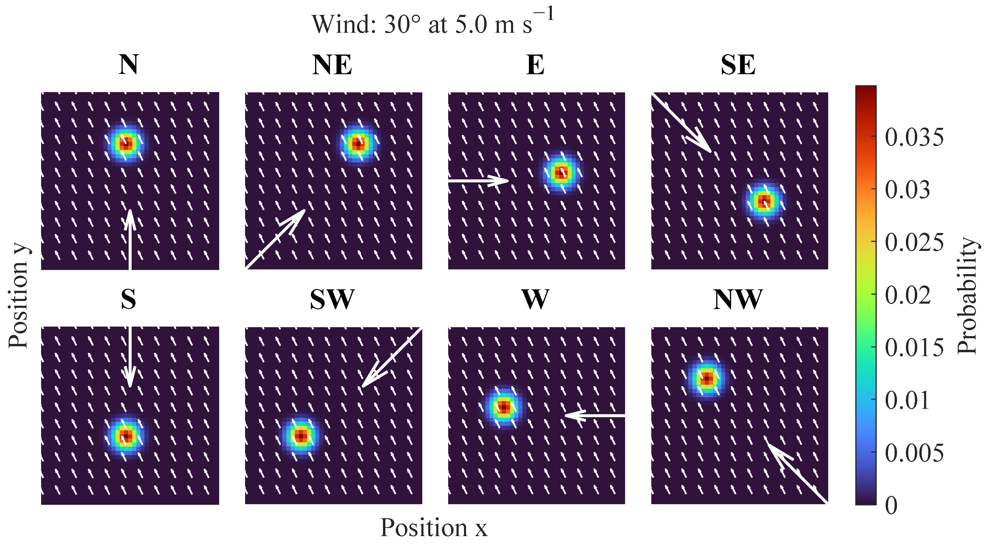
If a UAV failure occurs at the arrival cell b, the eventual crash site will be displaced from b due to ballistic descent dynamics and wind drift. To model the spatial distribution of potential impact locations, a directional impact-probability kernel $K_{\mathrm{dir}}$ is computed for each principal flight direction.

The horizontal fall distance is given by:

$$D_{\mathrm{fall}}=v_{\mathrm{UAV}}·t_{\mathrm{fall}},$$

(39)

where $t_{\mathrm{fall}}$ is the descent time and $v_{\mathrm{UAV}}$ the horizontal speed at failure.

Wind drift is modeled as:

$$\begin{array}{cccc}\hfill \Delta x_{\mathrm{wind}}& =⌊{\displaystyle \frac{v_{\mathrm{wind}}·t_{\mathrm{fall}}·cos{\chi }_{\mathrm{wind}}}{d_{\mathrm{cell}}}}⌉,\hfill & \hfill \Delta y_{\mathrm{wind}}& =⌊{\displaystyle \frac{v_{\mathrm{wind}}·t_{\mathrm{fall}}·sin{\chi }_{\mathrm{wind}}}{d_{\mathrm{cell}}}}⌉,\hfill \end{array}$$

(40)

with $d_{\mathrm{cell}}$ the grid resolution.

The expected impact location for direction “dir” is:

$$(x_{\mathrm{impact},\mathrm{dir}},y_{\mathrm{impact},\mathrm{dir}})=(x_b,y_b)+d_{\mathrm{dir}}·D_{\mathrm{fall}}+(\Delta x_{\mathrm{wind}},\Delta y_{\mathrm{wind}}),$$

(41)

where $(x_b,y_b)$ is the coordinate of arrival cell b and $d_{\mathrm{dir}}$ the unit vector of the travel direction.

A Gaussian kernel centered at the expected impact location represents the spatial dispersion of crash sites:

$$\begin{array}{cc}\hfill K_{\mathrm{dir}}(x,y)& =exp\left(-{\displaystyle \frac{r_{\mathrm{dir}}^2}{2{\sigma }^2}}\right),\hfill \end{array}$$

(42)

$$\begin{array}{cc}\hfill r_{\mathrm{dir}}& =\sqrt{{(x-x_{\mathrm{impact},\mathrm{dir}})}^2+{(y-y_{\mathrm{impact},\mathrm{dir}})}^2}.\hfill \end{array}$$

(43)

The kernel is normalized such that:

$$K_{\mathrm{dir}}(x,y)\leftarrow {\displaystyle \frac{K_{\mathrm{dir}}(x,y)}{{\sum }_{x,y}{K}_{\mathrm{dir}}(x,y)}}.$$

(44)

Figure 6 shows sample kernels for eight flight directions under a wind condition of 30° at 5 m/s⁻¹. Wind-induced drift causes a slight offset in the impact distributions.

For edge $(a\to b)$, the directional kernel $K_{\mathrm{dir}}$ is centered on the arrival cell b and overlaid on the inflated total fatality risk map $R_{\mathrm{total},\mathrm{infl}}(x,y)$ (Equation (38)). Only the overlapping cells ${\mathcal{V}}_b$ within the kernel footprint contribute to the risk.

The directional fatality risk for edge $(a\to b)$ is defined as:

$$R_{a\to b}=\sum _{(i,j)\in {\mathcal{V}}_b}{K}_{\mathrm{dir}}^{\left(b\right)}(i,j)·R_{\mathrm{total},\mathrm{infl}}(i,j),$$

(45)

where $K_{\mathrm{dir}}^{\left(b\right)}$ denotes the kernel translated to be centered on cell b. This quantity represents the expected consequence of a UAV failure at the arrival cell b when approaching from direction “dir”. The directional risk kernels illustrate that the point of failure and the actual ground impact location may differ due to wind effects. For conceptual clarity, a uniform wind field and radially symmetric distribution are assumed here, while noting that the kernel formulation can be adapted to different wind conditions or turbulence characteristics if more detailed aerodynamic or meteorological data are available.

5. Risk-Constrained UAV Pathfinding

We model the discretized operational area as a directed graph $\mathcal{G}=(\mathcal{V},\mathcal{E})$, where each node $v\in \mathcal{V}$ represents the center of a grid cell, and each directed edge $(a\to b)\in \mathcal{E}$ connects two adjacent cells in one of the eight principal movement directions. We formulate UAV trajectory planning as a discrete optimization problem on the directed motion graph $\mathcal{G}=(\mathcal{V},\mathcal{E})$. The decision variable is the path (sequence of nodes) $\pi \in \Pi (S⇝G)$ from start S to goal G:

$$\underset{\pi \in \Pi (S⇝G)}{min}{C}_G\left(\pi \right)=\sum _{(a\to b)\in \pi }\Delta {\tau }_{a\to b}$$

(46)

subject to the TLS and endurance constraints

$$T_G\left(\pi \right)\le \mathrm{TLS},C_G\left(\pi \right)\le {\mathcal{T}}_{max}.$$

(47)

Here, $C_G\left(\pi \right)$ denotes the cumulative flight time along the path and $T_G\left(\pi \right)$ the accumulated ground risk. The first constraint ensures that the induced risk of the selected trajectory does not exceed the predefined safety threshold, while the second constraint limits the total flight time to the available endurance ${\mathcal{T}}_{max}$.

We solve the above discrete optimization problem with an A* search procedure from a start node S to a goal node G, where each candidate node n is evaluated by a dynamically weighted cost function $f_n$. A* uses an optimistic time heuristic and balances flight time and accumulated risk under the TLS and endurance constraints. Since the weight between objectives adapts during the search, classical optimality conditions are not strictly met; we therefore regard the results as feasible, near-optimal solutions at practical runtimes. The choice of A* is further motivated by the combinatorial growth of path alternatives on an $N\times M$ grid with 8-directional moves ($\left|\mathcal{V}\right|=N·M$, $\left|\mathcal{E}\right|\approx 8\left|\mathcal{V}\right|$), where the number of distinct paths of length L may reach $8^L$. Exact constrained optimization is thus computationally demanding, justifying the use of a heuristic best-first method such as A*.

We introduce a simplified wind-aware endurance constraint, assuming steady, uniform wind and dependence only on course–wind alignment.

Let ${\mathcal{T}}_{max}$ be the available endurance (still-air equivalent at ground speed $v_{\mathrm{UAV}}$). With unit vectors $\widehat{\mathit{d}}\left({\chi }_{\mathrm{UAV}}\right)={[cos{\chi }_{\mathrm{UAV}},sin{\chi }_{\mathrm{UAV}}]}^{\top }$ and $\widehat{\mathit{w}}\left({\chi }_{\mathrm{wind}}\right)={[cos{\chi }_{\mathrm{wind}},sin{\chi }_{\mathrm{wind}}]}^{\top }$,

$$\begin{array}{cc}\hfill {\varphi }_{\mathrm{cons}}\left({\chi }_{\mathrm{UAV}}\right)& ={\displaystyle \frac{∥v_{\mathrm{UAV}}\widehat{\mathit{d}}\left({\chi }_{\mathrm{UAV}}\right)-v_{\mathrm{wind}}\widehat{\mathit{w}}\left({\chi }_{\mathrm{wind}}\right)∥}{v_{\mathrm{UAV}}}}\hfill \end{array}$$

(48)

$$\begin{array}{cc}\hfill & =\sqrt{1+{\left(\frac{v_{\mathrm{wind}}}{v_{\mathrm{UAV}}}\right)}^2-2\frac{v_{\mathrm{wind}}}{v_{\mathrm{UAV}}}cos\left({\chi }_{\mathrm{UAV}}-{\chi }_{\mathrm{wind}}\right)}.\hfill \end{array}$$

(49)

The endurance consumed on edge $(a\to b)$ with bearing ${\chi }_{\mathrm{UAV},a\to b}$ is

$$\Delta {\tau }_{a\to b}={\displaystyle \frac{d_{a,b}}{v_{\mathrm{UAV}}}}{\varphi }_{\mathrm{cons}}\left({\chi }_{\mathrm{UAV},a\to b}\right),d_{a,b}=d_{\mathrm{eucl}}(a,b).$$

(50)

Accumulated consumption to node n along the current path $\pi (S⇝n)$ is

$$C_n=\sum _{(u\to v)\in \pi (S⇝n)}\Delta {\tau }_{u\to v}.$$

(51)

To keep the search admissible, we use an optimistic heuristic that assumes the best alignment (max. tailwind), i.e., minimal factor i.e., ${min}_{{\chi }_{\mathrm{UAV}}}{\varphi }_{\mathrm{cons}}\left({\chi }_{\mathrm{UAV}}\right)=\left|1-\frac{v_{\mathrm{wind}}}{v_{\mathrm{UAV}}}\right|$:

$$h_{\mathrm{cons}}(n,G)={\displaystyle \frac{d_{\mathrm{eucl}}(n,G)}{v_{\mathrm{UAV}}}}\left|1-\frac{v_{\mathrm{wind}}}{v_{\mathrm{UAV}}}\right|.$$

(52)

We enforce endurance feasibility via a Big-M penalty:

$$f_n\leftarrow \left\{\begin{array}{cc}\mathcal{M},\hfill & \mathrm{if}{\mathcal{T}}_{max}-\left(C_n+h_{\mathrm{cons}}(n,G)\right)\le 0,\hfill \\ f_n,\hfill & \mathrm{otherwise}.\hfill \end{array}\right.$$

(53)

A sufficiently large $\mathcal{M}$ excludes infeasible nodes; alternatively, such nodes can be pruned outright. After applying the feasibility check, the remaining candidate nodes are evaluated using the cost function

$$f_n=(1-\omega )·{\displaystyle \frac{Q_n+h_{\mathrm{dist}}(n,G)}{{\eta }_{\mathrm{detour}}·d_{\mathrm{eucl}}(S,G)}}+\omega ·{\displaystyle \frac{T_n+h_{\mathrm{risk}}(n,G)}{\mathrm{TLS}}},$$

(54)

where:

• $Q_n$ is the accumulated path length from S to n,
• $h_{\mathrm{dist}}(n,G)$ is the Euclidean distance from n to G,
• $T_n$ is the accumulated directional fatality risk from S to n,
• $h_{\mathrm{risk}}(n,G)$ is the heuristic estimate of the remaining risk to G,
• ${\eta }_{\mathrm{detour}}\ge 1$ is the accepted detour factor relative to the straight-line distance,
• $\mathrm{TLS}$ is the target level of safety.

Here, the detour factor ${\eta }_{\mathrm{detour}}\ge 1$ expresses the operator’s acceptable detour relative to the straight-line distance and serves to normalize the distance term. It acts as a soft preference: trajectories longer than ${\eta }_{\mathrm{detour}}·d_{\mathrm{eucl}}(S,G)$ are not excluded, but they become progressively less favorable unless justified by lower induced risk. Feasibility remains governed by TLS and endurance constraints.

The cumulative risk $T_n$ at node n is computed by summing the risk accumulated along the path from S to the predecessor c and the additional edge risk when traversing $(c\to n)$:

$$T_n=T_c+T_{c\to n}^{\mathrm{edge}},$$

(55)

where the edge-specific contribution is given by:

$$T_{a\to b}^{\mathrm{edge}}={\lambda }_{\mathrm{fail}}·\Delta t_{a\to b}·R_{a\to b}.$$

(56)

which corresponds to the small-probability approximation $P_{\mathrm{fail}}\approx {\lambda }_{\mathrm{fail}}\Delta t$ of the exact expression $P_{\mathrm{fail}}=1-e^{-{\lambda }_{\mathrm{fail}}\Delta t}$. Here:

• ${\lambda }_{\mathrm{fail}}$ is the UAV-specific failure rate per unit time leading to an uncontrolled descent,
• $\Delta t_{a\to b}={\displaystyle \frac{d_{a,b}}{v_{\mathrm{UAV}}}}$ is the flight- or dwell time on edge from a to b,
• $R_{a\to b}$ is the directional fatality risk for edge $(a\to b)$ defined in Equation (45).

This definition directly links the graph-based path search with the directional fatality risk model: the spatial consequence term $R_{a\to b}$ from Equation (45) is scaled by the dwell time on edge from a to b and the event probability per unit time to obtain the edge risk contribution. The risk heuristic $h_{\mathrm{risk}}(n,G)$ is computed by sampling the cells along the straight line from n to G (using Bresenham’s algorithm [57]) and convolving their $R_{\mathrm{total},\mathrm{infl}}$ values with a Gaussian kernel aligned to the direct path, thus approximating the mean directional fatality risk to the goal. Analogous to the edge risk in Equation (56), the heuristic risk is scaled by the expected travel time and the per-second failure rate:

$$h_{\mathrm{risk}}(n,G)={\lambda }_{\mathrm{fail}}·{\displaystyle \frac{h_{\mathrm{eucl}}(n,G)}{v_{\mathrm{UAV}}}}·{\overline{R}}_{n\to G},$$

(57)

where:

• $v_{\mathrm{UAV}}$ is the UAV’s cruise speed,
• ${\overline{R}}_{n\to G}$ is the mean directional fatality risk along the direct line from n to G after Gaussian convolution.

The weight $\omega \in (0,1)$ is dynamically adapted during the search to shift towards risk avoidance if $T_n$ and $h_{\mathrm{risk}}(n,G)$ exceed the TLS:

$$\omega \leftarrow \left\{\begin{array}{cc}min(1-\epsilon ,\omega /(1-\zeta \left)\right),\hfill & \mathrm{if}{T}_n+h_{\mathrm{risk}}(n,G)>\mathrm{TLS},\hfill \\ max(\epsilon ,\omega ·(1-\zeta \left)\right),\hfill & \mathrm{otherwise},\hfill \end{array}\right.$$

(58)

The parameter $\zeta \in (0,1)$ defines the adaptation step size of the dynamic weight $\omega$. Its value should be chosen in relation to the grid resolution: for fine discretizations, smaller $\zeta$ values prevent abrupt reweighting over short distances, whereas larger values are required for coarser grids to maintain responsiveness. Very large $\zeta$ may lead to unstable behavior, while very small values can hinder the search from escaping local high-risk configurations.

This formulation allows the search to prioritize short paths when the risk heuristic $h_{\mathrm{risk}}(n,G)$ is well below the TLS, but progressively shift toward risk-averse routing as soon as the estimated total risk approaches or exceeds the TLS.

6. Simulation Setup and Data Sources

6.1. Parameters of the Unmanned Aerial Vehicle

For the risk assessment and pathfinding framework, key operational and physical parameters of the UAV must be defined. These parameters directly influence the impact energy, the ballistic descent model, the size of the directional impact kernels, and thus the computation of risk costs along edges in the graph. This study incorporates three exemplary UAV models [26] and assigns them to the corresponding classes C1 to C3 [58]. The key parameters $m_{\mathrm{UAV}}$, $S_{\mathrm{UAV}}$, and $c_D$ are summarized in

Table 2. UAV Parameters and average drag coefficient $c_D$ for all pitch angles [26].

UAV Type	UAV Mass	UAV Surface Area	Drag Coefficient
(Class)	${\mathit{m}}_{\mathbf{UAV}}$ [kg]	${\mathit{S}}_{\mathbf{UAV}}$ [m2]	${\mathit{c}}_{\mathit{D}}$
UAV 1 (C1)	0.75	0.0147	0.2670
UAV 2 (C2)	3.60	0.0667	0.1635
UAV 3 (C3)	11.00	0.2006	0.2225

.

Failure rates ${\lambda }_{\mathrm{fail}}$ for small UAVs vary significantly in the literature, with reported values ranging from 8 × 10⁻⁵ [19] and 1 × 10⁻⁴ [20] to 5 × 10⁻³ [21]. For the case study in this work, we assume a reliable UAV platform and set a uniform failure rate of

$${\lambda }_{\mathrm{fail}}=8 \times {10}^{-5}\mathrm{per}\mathrm{flight}\mathrm{hour}$$

for all UAV classes to enable a direct comparison of the influence of the UAV mass and other parameters on the resulting risk. Furthermore, we define a constant flight height $h_{\mathrm{UAV}}=30 \mathrm{m}$ with a cruise speed $v_{\mathrm{UAV}}=15 {\mathrm{m}/\mathrm{s}}^{-1}$. The endurance $e_{\mathrm{UAV}}=2000 \mathrm{s}$ is a constraint in the pathfinding to consider maximum mission durations. These parameters serve as initial assumptions for the proof of concept and can be adapted to a specific UAV configuration.

6.2. Simulation Setup for Synthetic Data

As cities have varying building densities and street layouts, random city tiles are generated to apply the risk map approach. Each city tile is a rectangular grid, in which the center of each cell is used as a potential waypoint for pathfinding. The resolution of this grid must be balanced, as a too-sparse grid may lead to lost information, and a too-dense grid pushes computational effort significantly. For our proof of concept, we use $r=2 \mathrm{m}$ and [1000, 1000] cells, resulting in a map area covering 2000 $\mathrm{m}$ by 2000 $\mathrm{m}$. This resolution represents a trade-off between capturing fine-scale structures such as sidewalks and maintaining a feasible runtime. While adaptive or irregular grids could, in principle, better reflect local urban layouts, the uniform discretization enables standardized heuristics and precomputed edge costs. Figure 7 visualizes a random city tile with its layer types. Street layers define areas of road traffic, sidewalks are pedestrian spaces, while buildings and trees provide additional sheltering.

For the street layers, different categories of streets can be generated, each requiring the following parameter set: The width describes the lateral extent of the street, the spacing defines the minimum distance between two streets of the same type to avoid cluttering, and the quantity of the street. Furthermore, the speed limit and road-traffic loads are generated for the risk assessment. Currently, we assume main and side streets as the two categories, with their selected parameters summarized in

Table 3. Street parameters for the map generation.

Type	Width	Spacing	Speed	Quantity	Road Traffic Load
	[m]	[m]	[km h−1]		[d−1]
Main	12	300	50	7	[15,000, 50,000]
Side	6	75	30	50	[100, 10,000]

. The streets are extruded on both sides by r to form the sidewalks.

Buildings are generated as rectangles with randomly selected edge lengths according to the minimum and maximum size and the height in

Table 4. Building and vegetation parameters for the map generation.

Type	Size	Height	Quantity	Energy Absorption
	[m]	[m]		${\mathit{E}}_{\mathbf{a}}$ [J]
Building	10, 100	20	400	13,558
Tree	3, 20	10	300	68

. Then, building parts intersecting with the streets or sidewalks are removed, and the remaining fragments are again checked to be above the minimum size. This avoids buildings either overlapping roads or being very small. The tree layer is generated similarly, but as circles with a radius of 3 $\mathrm{m}$. The values for $E_{\mathrm{a}}$ assume trees (‘wood joists’) and buildings (‘reinforced concrete’) [35].

The population is generated with a randomized density from 50 km⁻² to 4500 km⁻². This range spans typical densities from rural towns up to dense urban areas such as central districts. Let $s\sim \mathcal{U}(0,1)$ denote a uniformly distributed random variable representing the share of pedestrians, such that $(1-s)$ is the share of persons inside buildings.

6.3. Case Study with Real GIS Data

To demonstrate the applicability of the proposed method under realistic conditions, a case study was conducted for a representative urban area (centered around Dresden, Germany) using openly available geospatial data. The objective was to derive spatially resolved ground risk maps and compute safe UAV trajectories under real-world constraints.

To ensure general applicability, the workflow prioritizes open and globally accessible datasets such as OSM and public web services. Only where essential attributes were unavailable in OSM were supplemental regional datasets integrated. All vector layers were rasterized to a uniform grid with 5 $\mathrm{m}$ cell size.

Table A1. Overview of geospatial input layers and sources used in the case study.

Input Type	Source	Access/Tagging Criteria	Description/Use
Basemap Imagery	Federal Agency for Cartography and Geodesy	Web Map Service [64]	Visual reference for terrain and infrastructure
Road Network	OSM (via Overpass API)	key = highway AND value ∈ {motorway, trunk, primary, secondary, tertiary, unclassified, residential, motorway_link, trunk_link, primary_link, secondary_link, tertiary_link}	Road hierarchy (e.g., motorway, residential), maximum permissible speed, number of lanes, road width
Pedestrian Areas	OSM (via Overpass API)	(key = highway AND value∈ {living_street, pedestrian, footway}) OR key ∈ {amenity, leisure, public_transport, shop, cycleway, sidewalk, sport, tourism}	Outdoor locations with expected pedestrian presence during public or transit activities (e.g., sidewalks, squares, leisure and retail areas)
Sheltering Features	OSM (via Overpass API)	key = building OR (key = landuse AND value = forest) OR (key = natural AND value ∈ {tree, wood, tree_row})	Structures mitigating impact energy (e.g., buildings, vegetation)
Working Places	OSM (via Overpass API)	key = building AND value ∈ {commercial, office, industrial, college, goverment, hospital, kindergarten, museum, public, school, university}	Buildings with elevated daytime population (e.g., schools, hospitals, offices)
Population Density	Zensus 2022, Federal Statistical Office of Germany	2022 Zensus—Populations in grid cells (Version 2: 30 September 2024) [60].	Population counts per 100 $\mathrm{m}$ raster cell (2022 census)
Ground Traffic Data	City of Dresden—Office for Geodata and Cadastre	Web Feature Service [61]	Traffic volumes per road segment in vehicles/day
Elevation/Terrain	GeoSN—Saxony State Office for Geoinformation and Surveying	GeoTIFF download [59]	Surface height incl. vegetation/buildings (DOM1) and bare-earth elevation (DGM1)
Spatiotemporal Population Data	Federal Ministry of Transport and Digital Infrastructure	Statistical distribution based on national MiD 2017 travel survey [62]	Hourly population shares at home, work, or in public (MiD 2017)

summarizes the sources and characteristics of all datasets.

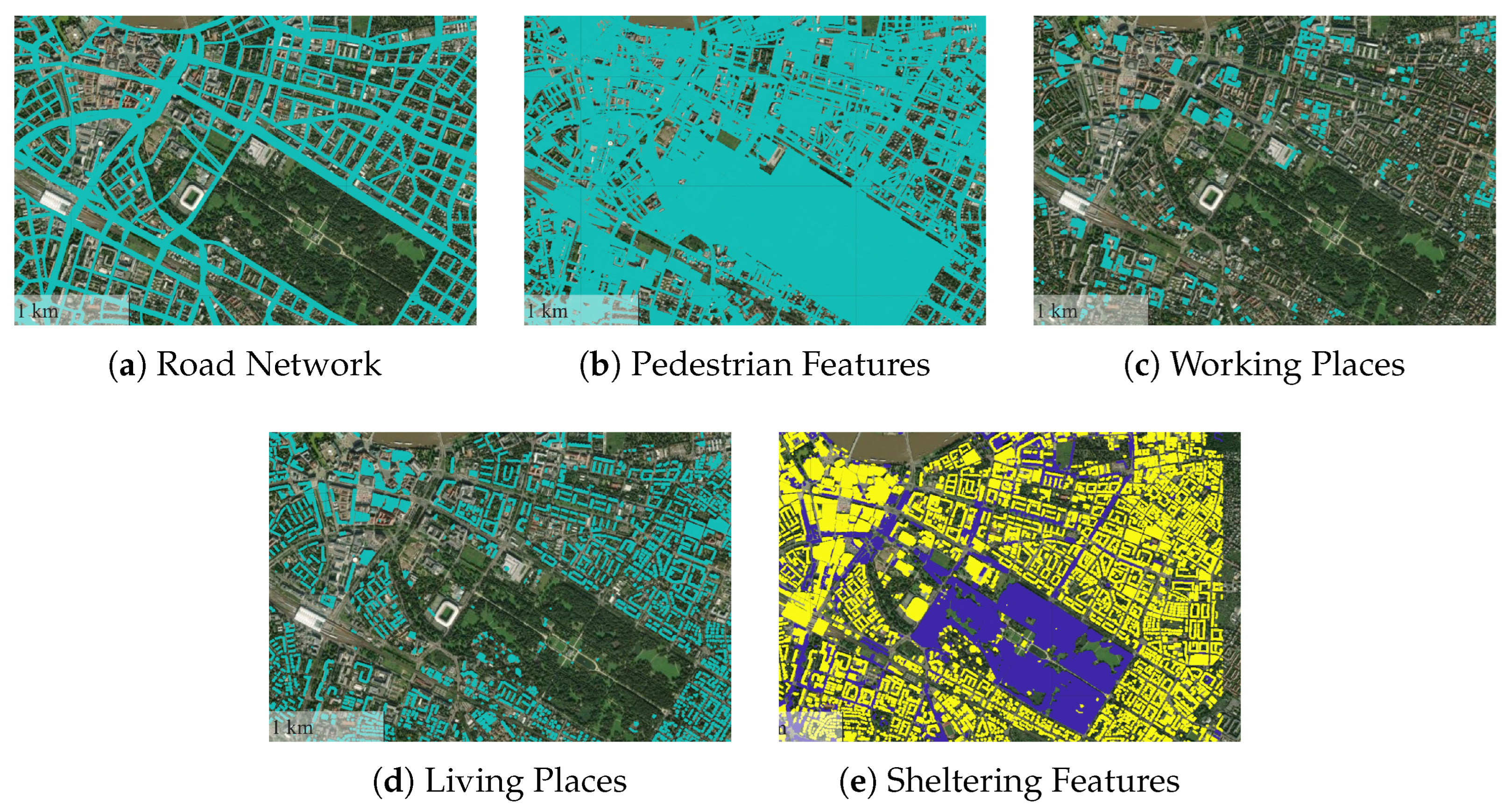
The core geoinfrastructure layers correspond to those in Section 6.2 and are illustrated in Figure 8:

• Road network for traffic-related fatality risk estimation (Section 4.4), including maximum permitted speed (interpolated where missing), road width, and number of lanes, all derived from OSM attributes.
• Pedestrian areas, working places, and living places to model the spatial distribution of persons. The pedestrian layer integrates area, line, and point features from OSM relevant to pedestrian presence. Area features (e.g., designated pedestrian zones) are rasterized directly. Linear features such as sidewalks, walking paths, and traffic-calmed streets are buffered prior to rasterization to approximate typical widths, as these are not consistently available in OSM. Generalized buffer radii are applied by infrastructure type (e.g., $4.5$ $\mathrm{m}$ for sidewalks and pedestrian zones, $2.4$ $\mathrm{m}$ for bicycle lanes). Point features such as public transport stops are similarly inflated to capture the surrounding zone of pedestrian activity. Buffer parameters can be adapted to local contexts or refined datasets if available.
• Sheltering features (buildings and vegetation) for risk reduction (Section 2.3). Building and forest polygons are rasterized directly, while point features representing individual trees are buffered using a generalized radius of $4.5$ $\mathrm{m}$.

All features were extracted from OSM via the Overpass API using the key–value combinations listed in Table A1.

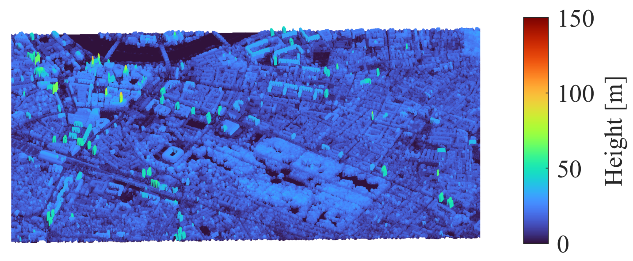
For impact energy estimation (Section 4.2), heights of the surface of the natural and artificial objects (e.g., vegetation, buildings, vehicles) were derived from the Digital Surface Model grid spacing 1 m (DOM1) and the Digital Terrain Model grid spacing 1 m (DGM1) provided by the Saxony State Office for Geoinformation and Surveying [59]. Subtracting the DGM1 from the DOM1 yields the Local Surface Elevation (LSE), representing the elevation of structures and vegetation above ground (Figure 9).

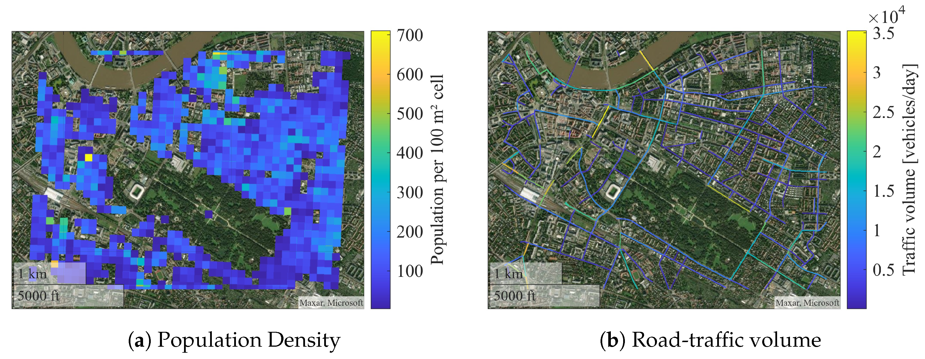
Population-density data were taken from the 2022 census [60] at 100 $\mathrm{m}$ grid resolution. Road-traffic data (vehicles/day) were obtained from the City of Dresden via Web Feature Service [61]. Figure 10 shows both datasets for the study area.

Since the exact real-time locations of persons and vehicles are unknown, their spatiotemporal distribution was estimated from empirical mobility data. Hourly presence shares for “home”, “work”, and “public/other” locations were taken from the German national travel survey (MiD 2017) [62] and mapped onto the corresponding geofeatures (Figure 8).

For residential areas, the census-based population per 100 $\mathrm{m}$ cell was proportionally allocated to the “living places” polygons within that cell, preserving the underlying census distribution. For non-residential features (e.g., working places, pedestrian areas), spatial smoothing kernels were applied to distribute the estimated number of persons according to the density of matching geofeatures. This assumes a higher local clustering of persons in areas where relevant geofeatures are spatially concentrated.

The total population within the map extent remains constant in each time step. Movements into or out of the area are not modeled; incorporating such flows would require additional datasets such as commuter statistics, which could in principle be integrated from origin–destination data where available [63].

7. Results

7.1. Synthetic Data Results

Our case study evaluates optimal pathfinding for the three UAV classes defined in Table 2 on procedurally generated city tiles, as described in Section 6.2. A statistical summary for $N=1034$ simulated runs is given in Figure 11. The left panel shows the distribution of relative risk reduction. UAV C1 and UAV C2 achieve mean reductions of $0.41$ and $0.43$, respectively, with median values of $0.41$ and $0.45$. UAV C3 yields the highest reduction on average (≈0.47, median ≈ 0.49), albeit with greater variability. The right panel depicts the Detour Factor (DF). Across all UAV classes, the mean DF ranges between $1.80$ and $1.84$, corresponding to detours of roughly 80% compared to the direct route. These comparatively high values result primarily from the orthogonal layout of streets and buildings: instead of diagonal shortcuts, trajectories are forced into horizontal and vertical segments to circumvent obstacles. Consequently, even in favorable cases, a detour of about 41% is inherently induced by the right-triangle relationship between grid-constrained paths and their diagonals, with additional length accumulating in complex urban layouts. From an operational perspective, the tolerability of such detours depends on the specific mission context and applicable requirements. Overall, 76.2% of trajectories satisfied the TLS constraint, with UAV C1 and UAV C2 reaching almost full compliance ($100\%$ and $95.5\%$), whereas UAV C3 achieved compliance in $35.7\%$ of cases, underlining the difficulty of meeting stringent safety thresholds in uniformly high-risk environments without excessive detours.

Table 5. Summary of TLS compliance for synthetic city tile simulations ($N=1034$).

UAV Class	Total Runs	Pass TLS Count	Pass TLS Rate
UAV 1 (C1)	341	341	1.000
UAV 2 (C2)	334	319	0.955
UAV 3 (C3)	359	128	0.357

summarizes, in condensed form, the total runs per UAV class, the number of successful runs meeting the TLS constraint, and the resulting pass rate.

The comparatively low pass rate for UAV C3 is primarily due to its larger mass and consequently higher induced ground risk, which significantly restricts available low-risk corridors in dense urban environments. In several simulations, the pathfinding algorithm accepted large detours to meet the $\mathrm{TLS}$, at times nearing the endurance limit.

This behavior can be explained by characteristics of the synthetic environments:

• Homogeneous high-risk clusters: Procedural generation occasionally produced large contiguous areas of elevated risk without intermediate safe cells, forcing extended detours.
• Extreme parameter combinations: Randomized city tiles sometimes combined high road-traffic density, high population density, and low building coverage—conditions unlikely to co-occur in real-world cities.
• Uniform street geometry: Orthogonal grid layouts reduce the availability of short alternative routes compared to the irregular street patterns of real cities.
• Strict grid movement: Even with 8-connectivity, blocked diagonals force stepwise zig-zag detours, amplifying path length.
• Low permeability of risk areas: Streets and sidewalks were modeled as sharply bounded high-risk features, eliminating partial traversal options that may exist in reality.

In contrast, real urban environments typically exhibit greater spatial heterogeneity, as road-traffic density, population exposure, and building coverage vary more gradually across the cityscape. This leads to a more diversified ground-risk distribution, creating localized low-risk corridors that the pathfinding algorithm can exploit. Such differentiation is largely absent in the synthetic environments, where homogeneous blocks of uniformly high risk frequently force excessive detours. These differences motivate the subsequent section, where the methodology is applied to a real-world GIS dataset.

7.2. Real GIS Data Results

To demonstrate the applicability of the proposed methodology and algorithms under realistic conditions, the approach was applied to real geospatial data for the selected urban study area from Section 6.3. Figure 12 shows the resulting spatial distribution of impact severity for UAV 1 (class C1, Section 6.1). Here, severity denotes the conditional probability of a fatal outcome given that a person or a stationary vehicle occupant is present in the respective grid cell at the moment of impact.

Panel (a) in Figure 12 shows the resulting terminal kinetic energy at ground level, calculated according to Section 4.2. High values appear in open areas where UAVs can fall unobstructed, while zones with tall buildings or dense tree coverage exhibit significantly lower terminal energies due to early impact with obstacles.

Panel (b) translates this energy field into the pedestrian fatality severity using the energy–fatality relationship from Equation (10). Sheltered zones within buildings or under dense vegetation appear in dark blue, indicating near-zero conditional fatality probability, while open street sections and plazas exhibit high values in red.

Panel (c) shows the impact severity for car occupants derived analogously via Equation (33), considering UAV impact energy and the maximum permitted vehicle speed per road segment (Section 4.4). High-severity areas follow the major road-traffic corridors, with broader and faster streets exhibiting the highest conditional fatality probability.

Figure 13 presents the rasterized spatial presence probabilities per cell for the selected analysis time of 16 $\mathrm{h}$. For pedestrian presence (Figure 13a), the activity shares home (39.54%), work (35.50%), commuting (15.79%), shopping (3.04%), leisure (4.10%), and other (2.03%) were interpolated from the MiD 2017 diurnal profile [60] and allocated to the corresponding geofeatures according to the procedure described in Section 6.3. High densities occur in compact residential and commercial areas, particularly in the city center and along major pedestrian corridors, whereas green spaces and sparsely built outskirts show low values.

Vehicle occupancy per cell (Figure 13b) was determined analogously based on road-traffic volume data obtained from the Web Feature Service [61] from Section 6.3. For streets without measured values, a two-dimensional interpolation was applied. Traffic volumes were scaled according to a generalized diurnal curve with two peaks at 6.5 $\mathrm{h}$ and 17 $\mathrm{h}$. From the resulting hourly flow rates, permissible speeds, and the spacing relations defined in Equations (26)–(28), probabilities were derived for a cell being occupied by a vehicle, lying within the stop distance, or being part of the leading hazard zone, cf. Figure 4.

By combining the impact severity distributions from Figure 12 with the spatial presence probabilities from Figure 13, we obtain the actual expected ground risk in the event of a UAV crash, as formulated in Section 4.3 and Section 4.4. The resulting pedestrian ground risk (Figure 14a) is computed according to Equation (10). Similarly, the traffic ground risk (Figure 14b) follows Equation (33). The two components are combined into the total ground risk (Figure 14c) following Equation (34). These ground risks represent a conditional probability given that a UAV has a failure over the respective cell; the multiplication by the UAV failure probability and the dwell time is performed in subsequent steps of the risk assessment framework (cf. Section 5).

In Figure 14a, elevated pedestrian risk is visible in densely built urban blocks and along major pedestrian corridors, while sheltered zones such as building interiors and heavily vegetated areas exhibit low values, as captured by the shielding factor in Equation (7). The traffic-related risk map in Figure 14b highlights main roads and intersections with high road-traffic volumes, where the likelihood of a vehicle being present at the moment of impact is greatest, as formulated in Equations (26)–(28). The combined total risk in Figure 14c reflects the additive nature of these two components, showing the highest values where high pedestrian and vehicle densities spatially coincide, consistent with Equation (34). In the examined urban scenario, road-traffic contributes the largest share to the overall risk, which should therefore be explicitly considered in route planning.

Following the inflation of the contingency volume described in Section 4.5 and the generation of directional ground risk maps (Section 4.6), the pathfinding algorithm from Section 5 was applied. For demonstration purposes, a sample trajectory was defined from the Faculty building to the riverbank, representing a challenging urban route crossing the dense city center. Figure 15 illustrates the resulting outputs. In panel (a), the optimized UAV trajectory (dashed line) for a TLS of ${10}^{-8}$ per flight is shown overlaid on the total ground risk map. Panel (b) presents the spatial distribution of aggregated induced ground risk along this optimized path, accounting for UAV failure probability, dwell time over each cell, and ballistic offset due to wind. Note that the colorbar limits differ from panel (a), as the multiplication with failure probability, dwell time, and spatial dispersion yields substantially smaller values. Panel (c) shows the corresponding aggregated risk for the direct-line connection between start and destination, again with adjusted colorbar scaling consistent with panel (b). Summing the induced risk contributions along the path yields the total mission-induced risk, which directly reflects the safety performance of the route.

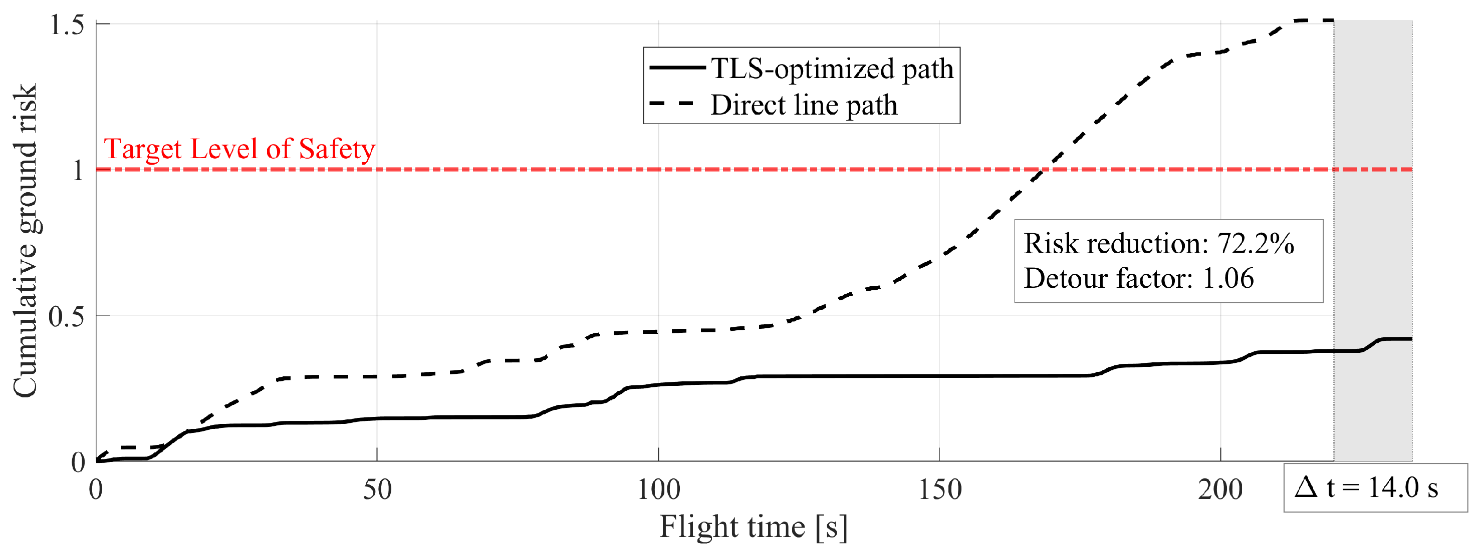
Figure 16 compares the cumulative induced ground risk over time for the optimized trajectory and the direct-line reference path. The optimized route results in only a marginally higher detour factor of $1.06$ and an additional flight time of $\Delta t=14.0 \mathrm{s}$, yet achieves a substantial reduction in total induced ground risk from $1.51\times {10}^{-8}$ to $4.71\times {10}^{-9}$, corresponding to a relative decrease of $72.2\%$. This reduction is primarily achieved by avoiding high-density street segments in the city center, crossing major roads at the shortest possible distance, and exploiting sheltering effects from buildings and vegetation along the route. Importantly, the optimized path remains well below the predefined TLS throughout the flight, whereas the direct path exceeds this threshold significantly during its final segment.

8. Conclusions and Outlook

This study demonstrates a scenario-specific approach to UAV path planning that explicitly incorporates the TLS into the routing decision. Unlike static risk assessments such as SORA [5], the proposed method evaluates route-specific risk for a given UAV, destination, and time-dependent ground conditions. The integration of ballistic descent modeling, wind drift, and sheltering effects enables a more realistic estimation of directional ground risk. Within the A* search, a dynamically adaptive cost function balances distance and risk, yielding paths that approach the TLS while maintaining operational efficiency. In the real-data case study, the heterogeneous spatial distribution of risk allowed for a significant relative reduction in induced ground risk by $72.2\%$ compared to the direct path, while the detour factor increased only to $1.06$–equivalent to an additional flight time of approximately 14 $\mathrm{s}$. These improvements were primarily achieved by avoiding dense, high-speed street sections, minimizing dwell time over road-traffic flows through perpendicular crossings of streets, and exploiting sheltering features.

The method exhibits good transferability from synthetic simulations to one representative real-world urban environment; however, its generalizability to other city typologies (e.g., high-rise districts or irregular street networks) remains to be evaluated, and several aspects require further development. The current implementation provides routing decisions based on a heuristic, which may not guarantee global optimality. Furthermore, this approach remains computationally demanding with average runtimes of about 331 $\min$ per simulation for risk maps with a high number of nodes (here ${10}^6$). Precomputed paths for fixed operational areas and times can reduce this burden. Further acceleration may be achieved through machine learning approaches, such as agent-based reinforcement learning or LSTM-based next-step prediction within a closed-loop planner. Future work could extend the risk model to additional ground entities, including rail and waterborne transport, and investigate the effect of more complex failure modes (e.g., partial rotor loss, parachute deployment) on descent dynamics. The contribution of ground vehicles to risk in this study is likely overestimated, as a deliberately conservative approach was applied when assessing both direct impacts and secondary accident effects. This requires further investigation through human factor studies and more detailed modeling of impact severity. For larger UAV such as air taxis, additional considerations will be necessary, including enhanced sheltering effects, cascading consequences, and group or societal risk. Finally, the current spatiotemporal population model does not capture inflow and outflow of commuters, nor infrequent mass events such as concerts or football matches. The integration of mobile network or road-traffic sensor data could substantially improve realism and will be addressed in future work.

The present study focuses exclusively on ground risk; air risk from potential conflicts with other airborne traffic is not considered yet. The proposed method is intended as part of the strategic flight planning process, conducted before the flight execution. The complementary tactical flight planning phase—addressing in-flight reactions to other airspace users, dynamic airspace changes, or sudden variations in ground conditions—will be investigated in subsequent stages of the project.

Finally, we note that applying a fixed TLS per flight inherently favors shorter trajectories, as the integrated risk scales with flight time under a constant failure rate. An alternative definition per flight hour could provide a more balanced metric for longer missions and can be readily implemented in our framework. Likewise, segment-specific failure probabilities (e.g., for take-off and landing versus cruise) could be integrated in future work, while these phases were abstracted in the present study.

References

1. European Commision. Commission Implementing Regulation (EU) 2019/947 of 24 May 2019 on the Rules and Procedures for the Operation of Unmanned Aircraft (Text with EEA Relevance). Official Journal of the European Union, L 152, 11 June 2019, pp. 45–71, 2019. Available online: https://eur-lex.europa.eu/eli/reg_impl/2019/947/oj/eng (accessed on 18 September 2025).
2. JARUS. JARUS Guidelines on Specific Operations Risk Assessment (SORA); Technical Report; Joint Authorities for Rulemaking on Unmanned Systems (JARUS): Edition 2.0, 2019. Available online: http://jarus-rpas.org/wp-content/uploads/2023/07/jar_doc_06_jarus_sora_v2.0.pdf (accessed on 18 September 2025).
3. International Civil Aviation Organization. Safety Management Manual, 4th ed.; Number 9859 in ICAO Doc; International Civil Aviation Organization: Montréal, QC, Canada, 2018. [Google Scholar]
4. Braßel, H.; Zeh, T.; Fricke, H.; Eltner, A. Optimal UAV Hangar Locations for Emergency Services Considering Restricted Areas. Drones 2023, 7, 203. [Google Scholar] [CrossRef]
5. European Union Aviation Safety Agency. Acceptable Means of Compliance (AMC) and Guidance Material (GM) to Commission Implementing Regulation (EU) 2019/947; Annex to ED Decision 2023/012/R, ed. 1, amend. 3; European Union Aviation Safety Agency: Cologne, Germany, 2023. [Google Scholar]
6. JARUS. JARUS Guidelines on Specific Operations Risk Assessment (SORA); Technical Report; Joint Authorities for Rulemaking on Unmanned Systems (JARUS): Edition 2.5, 2024. Available online: http://jarus-rpas.org/wp-content/uploads/2024/06/SORA-v2.5-Main-Body-Release-JAR_doc_25.pdf (accessed on 18 September 2025).
7. International Civil Aviation Organization. Advanced Surface Movement Guidance and Control Systems: (A-SMGCS) Manual, 1st ed.; ICAO: Montreal, QC, Canada, 2004. [Google Scholar]
8. Lin, X.; Fulton, N.; Westcott, M. Target Level of Safety Measures in Air Transportation—Review, Validation and Recommendations. In Proceedings of the IASTED International Conference Modelling, Simulation, and Identification (MSI2009), Beijing, China, 12–14 October 2009. [Google Scholar]
9. Dalamagkidis, K.; Valavanis, K.P.; Piegl, L.A. (Eds.) On Integrating Unmanned Aircraft Systems into the National Airspace System; Springer: Dordrecht, The Netherlands, 2012; Volume 54. [Google Scholar] [CrossRef]
10. Arterburn, D.; Ewing, M.; Prabhu, R.; Zhu, F.; Francis, D. FAA UAS Center of Excellence Task A4: UAS Ground Collision Severity Evaluation; Technical Report; Federal Aviation Administration: Washington, DC, USA, 2017.
11. Range Safety Group. Common Risk Criteria for National Test Ranges: Inert Debris; Technical Report ADA388624; Range Commanders Council: White Sands Missle Range, NM, USA, 2000. [Google Scholar]
12. Dalamagkidis, K.; Valavanis, K.P.; Piegl, L.A. On Unmanned Aircraft Systems Issues, Challenges and Operational Restrictions Preventing Integration into the National Airspace System. Prog. Aerosp. Sci. 2008, 44, 503–519. [Google Scholar] [CrossRef]
13. Bir, C.; Viano, D.C. Design and Injury Assessment Criteria for Blunt Ballistic Impacts. J. Trauma Acute Care Surg. 2004, 57, 1218–1224. [Google Scholar] [CrossRef]
14. Svatý, Z.; Vrtal, P.; Mičunek, T.; Kohout, T.; Nouzovský, L.; Frydrýn, M.; Blodek, T.; Kocián, K. Impact analysis assessment of UAS collision with a human body. PLoS ONE 2025, 20, e0320073. [Google Scholar] [CrossRef]
15. Shelley, A.V. A model of human harm from a falling unmanned aircraft: Implications for UAS regulation. Int. J. Aviat. Aeronaut. Aerosp. 2016, 3, 1. [Google Scholar] [CrossRef]
16. Clothier, R.; Walker, R.; Fulton, N.; Campbell, D. A casualty risk analysis for unmanned aerial system (UAS) operations over inhabited areas. In Proceedings of the AIAC12: 2nd Australasian Unmanned Air Vehicles Conference, Bristol UAV Conference, Melbourne, Australia, 19–22 March 2007; pp. 1–16. [Google Scholar]
17. Aalmoes, R.; Cheung, Y.; Sunil, E.; Hoekstra, J.; Bussink, F. A conceptual third party risk model for personal and unmanned aerial vehicles. In Proceedings of the 2015 International Conference on Unmanned Aircraft Systems (ICUAS), Denver, CO, USA, 9–12 June 2015; pp. 1301–1309. [Google Scholar]
18. Clothier, R.A.; Williams, B.P.; Hayhurst, K.J. Modelling the risks remotely piloted aircraft pose to people on the ground. Saf. Sci. 2018, 101, 33–47. [Google Scholar] [CrossRef]
19. Barr, L.C.; Newman, R.; Ancel, E.; Belcastro, C.M.; Foster, J.V.; Evans, J.; Klyde, D.H. Preliminary risk assessment for small unmanned aircraft systems. In Proceedings of the 17th AIAA Aviation Technology, Integration, and Operations Conference, Denver, CO, USA, 5–9 June 2017; p. 3272. [Google Scholar]
20. Osborne, M.; Lantair, J.; Shafiq, Z.; Zhao, X.; Robu, V.; Flynn, D.; Perry, J. UAS Operators Safety and Reliability Survey: Emerging Technologies towards the Certification of Autonomous UAS. In Proceedings of the 2019 4th International Conference on System Reliability and Safety (ICSRS), Rome, Italy, 20–22 November 2019; pp. 203–212. [Google Scholar] [CrossRef]
21. Pilko, A.; Sóbester, A.; Scanlan, J.P.; Ferraro, M. Spatiotemporal Ground Risk Mapping for Uncrewed Aircraft Systems Operations. J. Aerosp. Inf. Syst. 2023, 20, 126–139. [Google Scholar] [CrossRef]
22. La Cour-Harbo, A. Quantifying Risk of Ground Impact Fatalities for Small Unmanned Aircraft. J. Intell. Robot. Syst. 2019, 93, 367–384. [Google Scholar] [CrossRef]
23. Kim, S.H. Third-Party Risk Analysis of Small Unmanned Aircraft Systems Operations. J. Aerosp. Inf. Syst. 2020, 17, 24. [Google Scholar] [CrossRef]
24. Primatesta, S.; Rizzo, A.; La Cour-Harbo, A. Ground Risk Map for Unmanned Aircraft in Urban Environments. J. Intell. Robot. Syst. 2020, 97, 489–509. [Google Scholar] [CrossRef]
25. La Cour-Harbo, A. Ground impact probability distribution for small unmanned aircraft in ballistic descent. In Proceedings of the 2020 International Conference on Unmanned Aircraft Systems (ICUAS), Athens, Greece, 1–4 September 2020; pp. 1442–1451. [Google Scholar] [CrossRef]
26. Hammer, T.; Quitter, J.; Mayntz, J.; Bauschat, J.M.; Dahmann, P.; Götten, F.; Hille, S.; Stumpf, E. Free fall drag estimation of small-scale multirotor unmanned aircraft systems using computational fluid dynamics and wind tunnel experiments. CEAS Aeronaut. J. 2024, 15, 269–282. [Google Scholar] [CrossRef]
27. Che Man, M.H.; Haoliang, H.; Low, K.H. Crash Area Estimation for Ground Risk of Small Unmanned Aerial Vehicles Due to Propulsion System Failures. In Proceedings of the AIAA SCITECH 2022 Forum, San Diego, CA, USA, 3–7 January 2022. [Google Scholar] [CrossRef]
28. Bertrand, S.; Raballand, N.; Viguier, F. Evaluating Ground Risk for Road Networks Induced by UAV Operations. In Proceedings of the 2018 International Conference on Unmanned Aircraft Systems, Dallas, TX, USA, 12–15 June 2018; pp. 168–176. [Google Scholar] [CrossRef]
29. Huo, J.; Fu, X.; Liu, Z.; Zhang, Q. Short-term estimation and prediction of pedestrian density in urban hot spots based on mobile phone data. IEEE Trans. Intell. Transp. Syst. 2021, 23, 10827–10838. [Google Scholar] [CrossRef]
30. Jiang, R.; Cai, Z.; Wang, Z.; Yang, C.; Fan, Z.; Chen, Q.; Tsubouchi, K.; Song, X.; Shibasaki, R. DeepCrowd: A deep model for large-scale citywide crowd density and flow prediction. IEEE Trans. Knowl. Data Eng. 2021, 35, 276–290. [Google Scholar] [CrossRef]
31. Kim, Y.; Bae, J. Risk-Based UAV Corridor Capacity Analysis above a Populated Area. Drones 2022, 6, 221. [Google Scholar] [CrossRef]
32. Haklay, M.; Weber, P. Openstreetmap: User-generated street maps. IEEE Pervasive Comput. 2008, 7, 12–18. [Google Scholar] [CrossRef]
33. Zhou, S.; Liu, Y.; Zhang, X.; Dong, H.; Zhang, W.; Wu, H.; Li, H. Risk Assessment and Distribution Estimation for UAV Operations with Accurate Ground Feature Extraction Based on a Multi-Layer Method in Urban Areas. Drones 2024, 8, 399. [Google Scholar] [CrossRef]
34. Zhang, X.; Hao, H.; Ma, G. Laboratory test and numerical simulation of laminated glass window vulnerability to debris impact. Int. J. Impact Eng. 2013, 55, 49–62. [Google Scholar] [CrossRef]
35. Hardwick, M.J.; Hall, J.; Tatom, J.W.; Baker, R.G. Approved Methods and Algorithms for DoD Risk-Based Explosives Siting; Technical Report TR 14; U.S. Department of Defense Explosives Safety Board: Alexandria, VA, USA, 2009. [Google Scholar]
36. Che Man, M.H.; Haoliang, H.; Sivakumar, A.K.; Low, K.H. Preliminary Damage Severity Evaluation of Ground Vehicles and Covered Walkways under Collision with a Small Unmanned Aerial Vehicle (sUAV). In Proceedings of the AIAA AVIATION 2022 Forum, Chicago, IL, USA, 27 June–1 July 2022; American Institute of Aeronautics and Astronautics: Reston, VA, USA, 2022. [Google Scholar] [CrossRef]
37. Pang, B.; Hu, X.; Dai, W.; Low, K.H. UAV path optimization with an integrated cost assessment model considering third-party risks in metropolitan environments. Reliab. Eng. Syst. Saf. 2022, 222, 108399. [Google Scholar] [CrossRef]
38. Liu, B.; Xu, T.; Xu, X.; Wang, Y.; Sun, Y.; Li, Y. Energy absorption mechanism of polyvinyl butyral laminated windshield subjected to head impact: Experiment and numerical simulations. Int. J. Impact Eng. 2016, 90, 26–36. [Google Scholar] [CrossRef]
39. Xu, J.; Li, Y.B. Study of damage in windshield glazing subject to impact by a pedestrian’s head. Proc. Inst. Mech. Eng. Part D J. Automob. Eng. 2009, 223, 77–84. [Google Scholar] [CrossRef]
40. Aslan, M.F.; Durdu, A.; Sabanci, K. Goal distance-based UAV path planning approach, path optimization and learning-based path estimation: GDRRT*, PSO-GDRRT* and BiLSTM-PSO-GDRRT*. Appl. Soft Comput. 2023, 137, 110156. [Google Scholar] [CrossRef]
41. Sun, X.; Zhang, B.; Chai, R.; Tsourdos, A.; Chai, S. UAV trajectory optimization using chance-constrained second-order cone programming. Aerosp. Sci. Technol. 2022, 121, 107283. [Google Scholar] [CrossRef]
42. Rahman, M.M.H.; Al-Naeem, M.; Banerjee, A.; Sufian, A. EETO-GA: Energy Efficient Trajectory Optimization of UAV-IoT Collaborative System Using Genetic Algorithm. Appl. Sci. 2023, 13, 2535. [Google Scholar] [CrossRef]
43. Debnath, D.; Hawary, A.F.; Ramdan, M.I.; Alvarez, F.V.; Gonzalez, F. QuickNav: An Effective Collision Avoidance and Path-Planning Algorithm for UAS. Drones 2023, 7, 678. [Google Scholar] [CrossRef]
44. Hart, P.E.; Nilsson, N.J.; Raphael, B. A formal basis for the heuristic determination of minimum cost paths. IEEE Trans. Syst. Sci. Cybern. 1968, 4, 100–107. [Google Scholar] [CrossRef]
45. Lin, J.; Ye, F.; Yu, Q.; Xing, J.; Quan, Z.; Sheng, C. Research on Multi-UAVs Route Planning Based on the Integration of Improved Elastic Band and A-Star Algorithm. In Proceedings of the 2022 IEEE International Conference on Unmanned Systems (ICUS), Guangzhou, China, 28–30 October 2022. [Google Scholar] [CrossRef]
46. Du, Y. Multi-UAV search and rescue with enhanced A* algorithm path planning in 3D environment. Int. J. Aerosp. Eng. 2023, 2023, 8614117. [Google Scholar] [CrossRef]
47. Xu, L.; Xi, M.; Gao, R.; Ye, Z.; He, Z. Dynamic path planning of UAV with least inflection point based on adaptive neighborhood A* algorithm and multi-strategy fusion. Sci. Rep. 2025, 15, 8563. [Google Scholar] [CrossRef]
48. Zhang, X.; Liu, Y.; Gao, Z.; Ren, J.; Zhou, S.; Yang, B. A Ground-Risk-Map-Based Path-Planning Algorithm for UAVs in an Urban Environment with Beetle Swarm Optimization. Appl. Sci. 2023, 13, 11305. [Google Scholar] [CrossRef]
49. Tang, H.; Zhu, Q.; Qin, B.; Song, R.; Li, Z. UAV path planning based on third-party risk modeling. Sci. Rep. 2023, 13, 22259. [Google Scholar] [CrossRef]
50. Levasseur, B.; Bertrand, S.; Raballand, N.; Viguier, F.; Goussu, G. Accurate ground impact footprints and probabilistic maps for risk analysis of UAV missions. In Proceedings of the 2019 IEEE Aerospace Conference, Big Sky, MT, USA, 2–9 March 2019; pp. 1–10. [Google Scholar]
51. Lin, C.E.; Shao, P.C. Failure Analysis for an Unmanned Aerial Vehicle Using Safe Path Planning. J. Aerosp. Inf. Syst. 2020, 17, 358–369. [Google Scholar] [CrossRef]
52. Primatesta, S.; Scanavino, M.; Guglieri, G.; Rizzo, A. A Risk-based Path Planning Strategy to Compute Optimum Risk Path for Unmanned Aircraft Systems over Populated Areas. In Proceedings of the 2020 International Conference on Unmanned Aircraft Systems (ICUAS), Athens, Greece, 1–4 September 2020; pp. 641–650. [Google Scholar] [CrossRef]
53. Pilko, A.; Oakey, A.; Ferraro, M.; Scanlan, J. The Price of a Safe Flight: Risk Cost Based Path Planning. In Proceedings of the 2024 IEEE International Conference on Robotics and Automation (ICRA), Yokohama, Japan, 13–17 May 2024; pp. 3884–3890. [Google Scholar] [CrossRef]
54. Gao, Z.; Clarke, J.P.; Mardanov, J.; Marais, K. Developing 3D risk-informed no-fly zones for urban UAS operations. Aerosp. Sci. Technol. 2025, 163, 110297. [Google Scholar] [CrossRef]
55. International Civil Aviation Organization. Procedures for Air Navigation Services—Aircraft Operations, Volume I: Flight Procedures, 6th ed.; International Civil Aviation Organization (ICAO): Montréal, QC, Canada, 2018; ICAO Doc 8168; Volume I. [Google Scholar]
56. Runge, C. Ueber die numerische Auflösung von Differentialgleichungen. Math. Ann. 1895, 46, 167–178. [Google Scholar] [CrossRef]
57. Bresenham, J.E. Algorithm for computer control of a digital plotter. IBM Syst. J. 1965, 4, 25–30. [Google Scholar] [CrossRef]
58. European Commission. Commission Delegated Regulation (EU) 2019/945 of 12 March 2019 on Unmanned Aircraft Systems and on Third-Country Operators of Unmanned Aircraft Systems. Official Journal of the European Union, L 152, 11 June 2019, pp. 1–40, 2019. Available online: http://data.europa.eu/eli/reg_del/2019/945/oj (accessed on 18 September 2025).
59. GeoSN—Saxony State Office for Geoinformation and Surveying. Digital Surface Model (DOM1) and Digital Terrain Model (DGM1), 2024. Available under the Data License Germany—Attribution—Version 2.0 (dl-de/by-2-0). Source: GeoSN, dl-de/by-2-0. Available online: https://www.geodaten.sachsen.de/digitale-hoehenmodelle-3994.html (accessed on 16 July 2025).
60. Statistische Ämter des Bundes und der Länder. Zensus 2022—Bevölkerungszahlen in Gitterzellen, 2nd ed.; Federal Statistical Office of Germany: Wiesbaden, Germany, 2024. [Google Scholar]
61. City of Dresden–Office for Geodata and Cadastre. Traffic Volume Data (Vehicles per Day) from the Thematic City Map. 2024. Available online: https://stadtplan.dresden.de (accessed on 10 July 2025).
62. Nobis, C.; Kuhnimhof, T. Mobilität in Deutschland—MiD Ergebnisbericht. A Study by Infas, DLR, IVT and Infas 360 on Behalf of the Federal Ministry for Transport and Digital Infrastructure (FE-Nr. 70.904/15). Chapter 7, Figure 7: Weekly Patterns of Population Locations. Bonn, Germany, 2018. Available online: https://www.mobilitaet-in-deutschland.de (accessed on 5 June 2025).
63. Statistische Ämter der Länder. Qualitätsbericht, Pendlerrechnung der Länder, Stand: 16.10.2024; Technical Report; Information und Technik Nordrhein-Westfalen (IT.NRW); Statistisches Landesamt, im Auftrag der Statistischen Ämter der Länder: Düsseldorf, Germany, 2024. [Google Scholar]
64. Federal Agency for Cartography and Geodesy (BKG). basemap.de Web Raster (WMS Service). © GeoBasis-DE/BKG. 2024. Available online: https://www.bkg.bund.de (accessed on 21 July 2025).
Figure 1. Example of the geographical zones restricting UAV operation in the downtown area of Dresden, Germany.
Drones 09 00666 g001
Figure 2. Bow-tie diagram for an uncontrolled descent of a UAV. On the left side, the fault tree indicates a partial list of safety events and potential preventive barriers. On the right side, potential outcomes are shown considering persons outside as pedestrians and in vehicles.
Drones 09 00666 g002
Figure 3. Log-normal-distributed probability for pedestrian fatalities depending on the body part and kinetic energy [11].
Drones 09 00666 g003
Figure 4. Definition of hazard zones in front and on top of a passenger car.
Drones 09 00666 g004
Figure 6. Impact probability distributions for UAV failures in eight flight directions under wind influence (30° at 5 m/s−1). Large arrows indicate the direction of UAV motion; small arrows show the wind vector field.
Drones 09 00666 g006
Figure 7. Layer samples of the random city generation.
Drones 09 00666 g007
Figure 8. Geospatial features used for population likelihood modeling: (a) Road Network, (b) Pedestrian infrastructure, (c) Working place indicators, (d) Residential areas, and (e) Sheltering characteristics. In (e), buildings are shown in yellow, while vegetation such as trees, groups of trees, and forest areas are shown in blue.
Drones 09 00666 g008
Figure 9. Derived Local Surface Elevation (LSE) from DOM1–DGM1.
Drones 09 00666 g009
Figure 10. Comparison of (a) population density [60] and (b) road-traffic volume [61].
Drones 09 00666 g010
Figure 11. Statistical distribution for N = 1034 simulated runs of (left) relative risk reduction and (right) detour factor across all simulation runs for UAV classes C1–C3. Red lines indicate median values; whiskers extend to 1.5 × the interquartile range.
Drones 09 00666 g011
Figure 12. Spatial distribution of impact severity for UAV 1 (class C1): (a) terminal impact energy, (b) derived pedestrian fatality severity, and (c) derived fatality severity for occupants of stationary vehicles.
Drones 09 00666 g012
Figure 13. Rasterized spatial presence probability per cell at 16 h : (a) pedestrians and (b) ground vehicles, derived from population and road-traffic data.
Drones 09 00666 g013
Figure 14. Spatial distribution of expected ground risk in the case of a UAV crash, derived from impact likelihood and severity: (a) pedestrians, (b) vehicles, and (c) total risk.
Drones 09 00666 g014
Figure 15. TLS-constrained UAV routing for a target safety level of 10 8 per flight: (a) optimized trajectory over ground risk map, (b) aggregated induced ground risk along optimized path, and (c) along direct-line path. Exposure maps account for UAV failure probability, dwell time, and ballistic offset due to wind.
Drones 09 00666 g015
Figure 16. Cumulative induced ground risk over flight time for the optimized UAV trajectory (solid) and the direct-line reference path (dashed). The red line marks the TLS; the textbox indicates risk reduction and detour factor.
Drones 09 00666 g016