Article

Intelligent Trajectory Prediction Algorithm for Hypersonic Vehicle Based on Sparse Associative Structure Model

by
Furong Liu
,
Lina Lu
*,
Zhiheng Zhang
,
Yu Xie
and
Jing Chen
College of Intelligence Science and Technology, National University of Defense Technology, Changsha 410073, China
*
Author to whom correspondence should be addressed.
Drones 2024, 8(9), 505; https://doi.org/10.3390/drones8090505
Submission received: 12 August 2024 / Revised: 15 September 2024 / Accepted: 17 September 2024 / Published: 19 September 2024
(This article belongs to the Collection Drones for Security and Defense Applications)

Abstract

:
The Hypersonic Glide Vehicle (HGV) has become a focal point in military competitions among nations. Predicting the real-time trajectory of an HGV is of significant importance for aerospace defense interception and assessing enemy combat intentions. Existing prediction methods are limited by the need for large data samples and poor general applicability. To address these challenges, this paper presents a novel trajectory forecasting approach based on the Sparse Association Structure Model (SASM). The SASM can uncover the relationship among known data, transfer associative relationships to unknown data, and improve the generalization of the model. Firstly, a trajectory database is established for different maneuvering modes based on the six-degree-of-freedom motion equations and models of attack and bank angles of the HGV. Subsequently, three trajectory parameters are selected as prediction variables according to the maneuvering characteristics of the HGV. A parameters prediction model based on the SASM is then constructed to predict trajectory parameters. The SASM model demonstrates high accuracy and generalization in forecasting the trajectories of three different HGV types. Experimental results show a 50.35% reduction in prediction error and a 48.7% decrease in average processing time compared to the LSTM model, highlighting the effectiveness of the proposed method for real-time trajectory forecasting.

1. Introduction

The hypersonic gliding vehicle (HGV) is now a key focus in global military research due to its deep penetration, precision strikes, and high maneuverability. As hypersonic technology competition grows, real-time HGV trajectory prediction is essential for aerospace defense and combat intent analysis [1,2].
Within the domain of trajectory prediction, present methodologies are primarily categorized based on the nature of the targets being predicted. The first category pertains to low-altitude, low-speed targets, including conventional aviation aircraft and unmanned aerial vehicles (UAVs) [3,4]. These entities exhibit moderate velocities, predictable flight paths, and are supported by an abundance of data conducive to analytical studies. The extant scholarly research has predominantly utilized techniques such as deep learning algorithms [4,5], machine learning models [6], and database matching [7] to discern and exploit the regularities within their flight paths. Conversely, the second category addresses high-altitude, high-velocity targets, which are exemplified by ballistic missiles. Despite their rapid pace, these targets adhere to more consistent motion dynamics [8,9]. Leveraging this predictability, researchers have applied a suite of analytical tools, including analytical solutions [9,10], numerical integration techniques [11,12], and regression analysis methods [13], to precisely determine their trajectories.
However, HGV targets operate at significantly higher speeds than conventional aircraft, lacking predefined flight routes and mission-specific characteristics, along with limited historical trajectory data. Consequently, the majority of the existing algorithms for predicting trajectories are predicted on the offensive standpoint [14,15,16], with a dearth of studies addressing the defensive perspective. The extant methodologies for trajectory prediction can be broadly classified into three distinct categories: based on standard control models, based on inference from combat intentions and grounded in parameter identification techniques.
The first method hinges on the assumption that HGVs execute maneuvers within the confines of established control models, thereby delineating their motion trajectories. Li et al. [17] have delved into predicting HGV trajectories under such typical control laws, achieving commendable prediction accuracy. Nonetheless, this approach is decided on specific modes, limiting the generalization capabilities of the prediction model. A method that depends on intention inference is centered on discerning the adversary’s strategic objectives, aiming to forecast the trajectory by simulating the target’s strike path. Li et al. [18] introduced a multimodel and multi-intention fusion approach based on Bayesian inference. This dual-layer fusion strategy amalgamates diverse maneuvering patterns and intentions, enhancing the precision and resilience of the trajectory forecasts. Although this method offers significant strategic insights, integrating attack intentions with dynamic battlefield conditions and quantifying the importance of various qualitative elements remain as challenges.
The last method based on parameter identification emphasizes the identification and representation of control parameter information for the HGV. According to learning the variation law of the lift-to-drag ratio, Wang et al. [19] have employed curve fitting techniques to facilitate trajectory forecasting. While their approach adeptly integrates the lift-to-drag ratio with the target’s state for predictive purposes, its utility is confined to the longitudinal plane and does not extend to three-dimensional trajectories. Zhai et al. [20] pioneered the definition of a novel suite of aerodynamic parameters, fitting them via the least squares method, thereby achieving 3D trajectory prediction. However, this methodology has limitations in conditions of nonlinear aerodynamic scenarios, such as abrupt alterations in the aircraft’s aerodynamic properties. Further advancing the field, Zhang et al. [21] introduced an ensemble empirical mode and attention long short-term memory (LSTM) network, harnessing the ability of neural networks to model nonlinear aerodynamic accelerations. This innovative approach, while effective, necessitates extensive datasets for training to ensure robust performance.
It is evident that current research methodologies have several limitations:
  • Traditional linear fitting methods, such as the least squares method, often struggle to accurately represent parameters with nonlinear characteristics. Meanwhile, deep learning techniques, though predictive, often necessitate a vast amount of trajectory data, which is not feasible in practical scenarios;
  • Most methods are built upon the premise that control quantities or parameters adhere to specific patterns, thereby limiting their versatility and adaptability across diverse contexts.
Given the inherent nature of HGV trajectory prediction as a time-series task, this study frames it as a transfer learning problem from historical to future trajectories. We propose addressing existing limitations by introducing methods from time-series domain adaptation.
The primary contributions of this paper are as follows:
(1)
Based on the motion model of an HGV, we devise a rapid trajectory generation method tailored for various maneuvering patterns, thereby establishing a comprehensive trajectory dateset of the HGV.
(2)
This paper introduces a trajectory parameter prediction method grounded in the Sparse Associative Structure Model (SASM) [22]. We are the first to apply the SASM from the field of time domain adaptation to HGV trajectory prediction. Compared to traditional methods, the proposed method can harness the deep learning capability of the SASM, adeptly uncovering the intricate interplay between established state variables and the predictive variables that shape a trajectory. By distilling and transferring these associative relationships, the accuracy of our method is greatly improved compared to some mainstream algorithms. This innovation enhances the adaptability and predictive prowess of our model, offering a more efficient and effective solution for trajectory prediction.
The rest of the paper is organized as follows. A method to generate HGV trajectory quickly in various maneuvering patterns is designed in Section 2. Section 3 utilizes the dynamic equations of the HGV to dissect its maneuverability characteristics and strategically selects parameters that are crucial for trajectory prediction. In Section 4, an SASM trajectory parameter prediction algorithm is devised, accompanied by a detailed explanation of its implementation ideas and measures. Section 5 presents the simulation experiments conducted to evaluate the performance of the proposed algorithm, while Section 6 offers a comprehensive conclusion of the paper.

2. Generation of HGV Trajectory Dataset

In this section, leveraging the motion model, attack angle model, and bank angle model, we introduce a method aimed at generating a vast array of HGV trajectories in diverse maneuvering patterns. This approach enables the creation of a comprehensive dataset for further analysis and utilization.

2.1. Motion Equation of HGV

Assuming the earth as a uniform sphere and neglecting its rotation, the six-degree-of-freedom motion equations [23] of a hypersonic glide vehicle in the velocity time coordinate (VTC) system can be expressed as in Equation  (1).
r ˙ = V sin θ λ ˙ = V cos θ sin σ r cos ϕ ϕ ˙ = V cos θ cos ψ r V ˙ = a D g sin θ θ ˙ = 1 V a L cos ν + V 2 r g cos θ ψ ˙ = 1 V a L sin ν cos θ + V 2 r cos θ sin σ tan ϕ
where λ , ϕ , r, V, θ , and σ are the state variables of the aircraft representing longitude, latitude, geocentric distance, velocity, flight path angle, and heading angle, respectively. α and ν are the control variables representing the angle of attack and the bank angle, respectively. The above parameters are explained in Table A1 of the Appendix A. And location relationships between angles are shown in the Figure 1. a L and a D denote lift and drag acceleration, respectively, as shown in Equation (2).
a L = L m = ρ V 2 S C L ( α ) 2 m a D = D m = ρ V 2 S C D ( α ) 2 m
where S and m denote the characteristic area and mass of the vehicle. C L is the aerodynamic lift coefficient, while C D is the drag coefficient. The above parameters are influenced by the attack angle α . ρ is the atmospheric density.

2.2. Attack Angle Model and Bank Angle Model

Given the high initial velocity of the HGV, they often utilize a large angle of attack during the initial phase to reduce the thermal flux density and meet the constraints. To achieve the maximum range, the vehicle typically adopts a glide with the highest lift-to-drag ratio. Consequently, a velocity-based attack angle model is employed for the generation of trajectories in longitudinal jumping gliding [24]:
α = α max , if V V 1 , α K α max V 2 V 1 ( V V 1 ) + α max , if V [ V 1 , V 2 ) , α K , if V < V 2 .
where K = L / D is the lift-to-drag ratio, and α max is the biggest attack angle corresponding to the maximum lift-to-drag ratio. α max is the maximum attack angle. V 2 and V 1 represent the upper and lower limits of the velocity range over which the angle of attack varies, and these can be adjusted to meet the specific requirements of the flight trajectory.
The bank angle is explicitly included in the motion Equation (1), and its variation directly affects the trajectory inclination and azimuth of the aircraft, determining the aircraft’s lateral maneuvering mode. Disregarding the brief period required for the sideslip angle to change, we employ an alternating square wave to simulate the lateral maneuvering model of the HGV.
We present a bank angle model, which is a piecewise function of time that is represented as follows:
ν = 1 n 1 f ν max , i f t T moving n , 0 < n N , ν 0 , i f t T other
where ν 0 is the bank angle in the state of nonmaneuvers, while ν max denotes the maximum bank angle. f is the initial direction of the lateral maneuver, with values being either 1 or −1. n represents the number of times the aircraft has currently maneuvered laterally. T moving n is the time range of the nth lateral maneuver.

2.3. Trajectory Generation Process

In the trajectory generation process for a hypersonic glide vehicle, the corresponding control equations are first selected based on different maneuvering modes. Then, the initial state of the HGV and the initial values of the control quantities are given. Based on the control equations, as well as the attack angle and bank angle, the control quantities at the corresponding times are calculated. Finally, the trajectory is obtained through integration. The process of generating the maneuver trajectory for HGVs is illustrated in Figure 2.

3. Trajectory Parameters Selection

In this section, from a defensive perspective, we conduct an in-depth analysis of the maneuverability inherent to HGVs by leveraging the equation of motion. This analysis serves as a pivotal foundation for the judicious selection of parameters crucial for the trajectory prediction model.

3.1. Analysis of Maneuver Characteristics

The primary trajectory of an HGV can be segmented into a longitudinal and a lateral trajectory, resulting from the interplay between longitudinal and lateral maneuvers.

3.1.1. Analysis of Longitudinal Maneuver

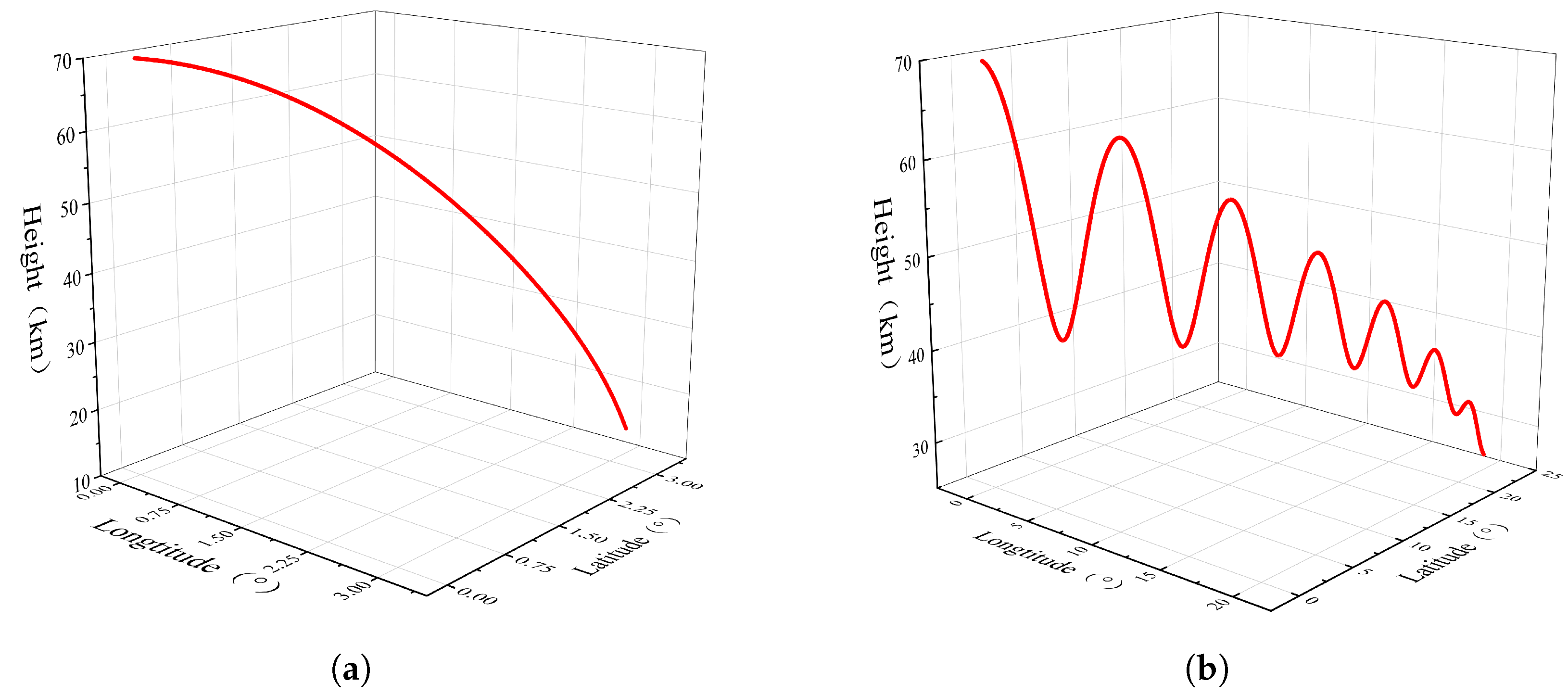
Longitudinal maneuvers are predominantly influenced by gravitational forces and aerodynamic lift, which include two distinct states: a jumping gliding state and a balanced gliding state, as depicted in Figure 3.
In the state of balanced glide, the forces acting on the HGV in the longitudinal direction are perfectly counterbalanced, resulting in a zero rate of change for the flight path angle. The equilibrium gliding condition can be expressed as follows:
a L cos v + V 2 r g cos θ = 0
Should the equilibrium conditions for balanced gliding not be met, the HGV may transition into a state of jumping gliding. The HGV can modify its jump amplitude and jump frequency by adjusting the attack angle. To enhance the penetration capability of the HGV, the jumping gliding maneuver is commonly employed. Consequently, this paper primarily delves into the investigation of the jumping gliding state.

3.1.2. Analysis of Lateral Maneuvers

The bank angle ν plays a crucial role in the flight of a hypersonic glide vehicle, enabling the decomposition of the lift force into components that aid in climbing and turning. By strategically manipulating the bank angle, the vehicle can execute diverse lateral maneuver patterns, including the C-shape and S-shape maneuvers, thus enhancing its overall maneuverability. While lateral maneuvers do not directly reduce the kinetic energy consumption of the HGV or increase its range, they do have the potential to increase the probability of being intercepted [25].
Specifically, when the rank angle is set to zero, the turning force component vanishes, resulting in the absence of lateral maneuvering by the vehicle. The C-shaped maneuver typically involves a single left turn or right turn, which is characterized by a relatively stable flight path. During this maneuver, the bank angle is generally set to a constant value to maintain the lateral direction of the HGV. In contrast, the S-shaped maneuver involves multiple turns in the lateral direction, which enhances the vehicle’s maneuverability. During an S-shaped maneuver, the bank angle needs to be reversed several times to achieve the desired trajectory with multiple turns.
The aerodynamic turning a T and climbing acceleration a C play pivotal roles in the lateral maneuvering of an aircraft. Their expressions are shown in Equation (6). When a T > 0, the aircraft banks to the left; conversely, it banks to the right. When a C > 0, the aircraft climbs up; otherwise, it dives down.
a T = a L sin ν a C = a L cos ν

3.2. Selection of Trajectory Parameters

In the selection of trajectory prediction parameters, it is essential to consider two critical aspects: (1) the extent to which the parameters incorporate control information for the aircraft and (2) the degree to which the parameters display a stable and predictable pattern of variation suitable for mathematical formulation.
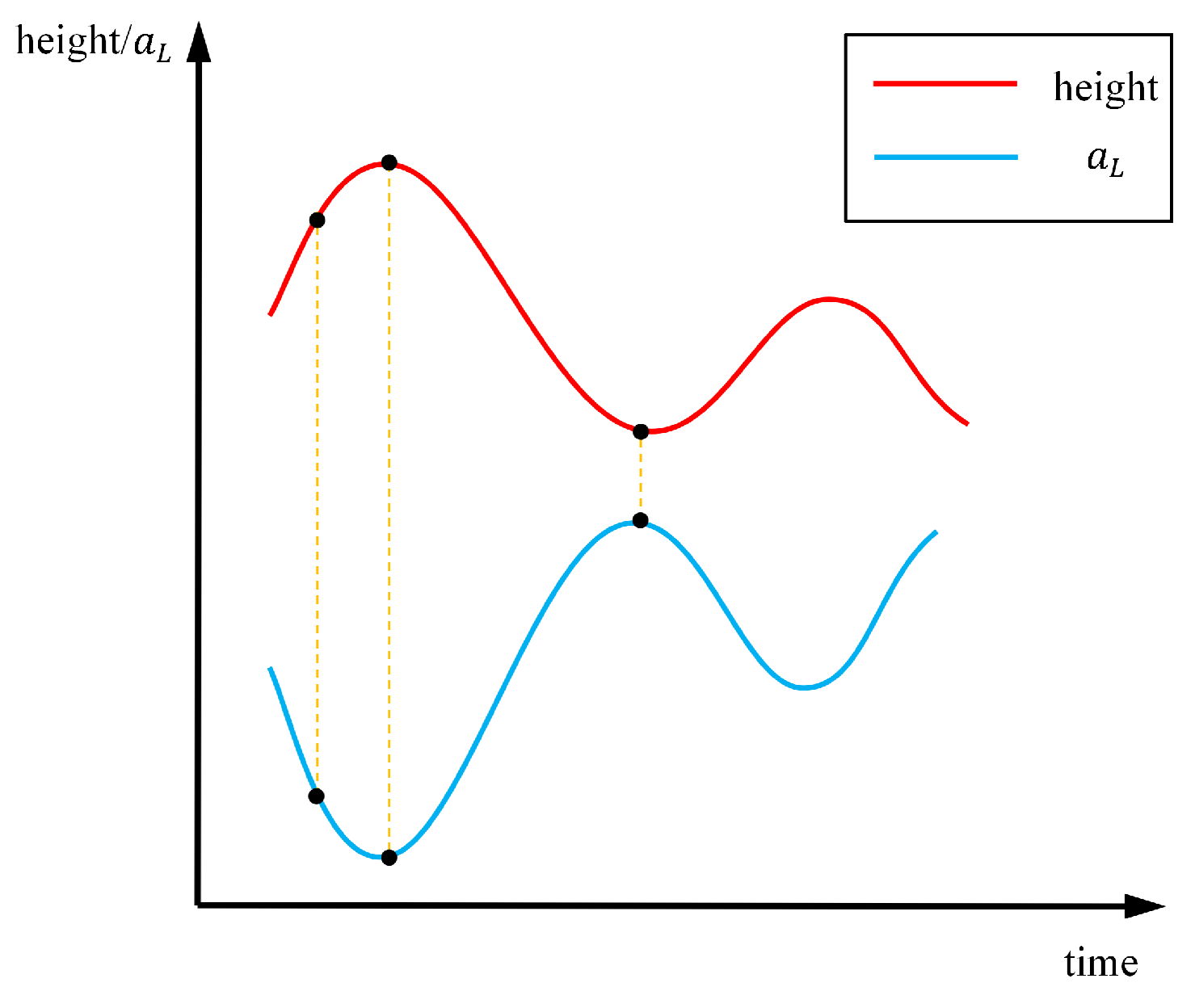
Based on Equation (2), the aerodynamic lift and drag accelerations include both control variables and additional unknowns, such as the vehicle’s mass and surface area. Consequently, we can utilize the aerodynamic acceleration and status information of the HGV to reconstruct its trajectory. In general, the aerodynamic acceleration maintains a consistent pattern of variation. During the jumping gliding state, the HGV is predominantly influenced by gravity, aerodynamic lift, and aerodynamic drag. As the HGV ascends, the air density diminishes with increasing altitude, which in turn leads to a progressive reduction in lift. Once the aircraft reaches a specific height, it decelerates to a standstill under the combined effects of gravity and aerodynamic resistance, subsequently commencing its descent. Conversely, as the HGV descends and the altitude decreases, the air density increases, augmenting the aerodynamic lift. At a critical lower altitude, the net force acting on the HGV becomes directed upwards, causing the descent velocity to gradually diminish to zero. Subsequently, the HGV ascends once more, thereby completing a cycle of oscillatory motion characteristic of jumping gliding. Therefore, the aerodynamic lift and drag acceleration exhibit a similar sinusoidal or cosine periodic variation pattern, with the amplitude of oscillation demonstrating a tendency towards attenuation—as depicted in Figure 4.
As delineated in Section 3.1.2, the aerodynamic turning and climbing accelerations are identified as the primary determinants of the lateral maneuverability of an HGV. Analysis of Equation (6) elucidates that the variation in the bank angle directly influences the turning acceleration and climb acceleration of an aircraft, which control an HGV’s lateral maneuverability. Consequently, we selected the lift acceleration, drag acceleration, and bank angle as predictive parameters for the trajectory modeling of an HGV.

4. Prediction Method

In this section, we firstly introduce the principles of the Sparse Associative Structure Model (SASM). Then, we propose the trajectory parameters prediction method based on the SASM, and we articulate the comprehensive framework for HGV trajectory prediction.

4.1. SASM Algorithm

Given that trajectory sequences inherently possess the nature of time series, it is feasible to incorporate adaptive methodologies from time domain into the prediction of aircraft trajectory parameters. Traditional time series processing methods, such as RNN and LSTM, may fail to capture the interconnections between variables, which can limit their ability to generalize from the training data to unseen data. To address this, we have employed a deep learning approach grounded in causal inference—the Sparse Associative Structure Model (SASM). This model eliminates spurious correlations and enhances model generalization and accuracy.
The core philosophy of the SASM lies in leveraging the principle of causal sparsity to relax causal relationships into sparse associative structures. Subsequently, it harnesses the sequential representation and association capturing prowess of deep learning, accomplishing the reconstruction of sparse association structures as a means to approximate causal discovery. The model primarily comprises two components: adaptive sequence representation and sparse association structure discovery, as illustrated in Figure 5.

4.1.1. Adaptive Sequence Representation

Due to the fact that time series inputs are constantly changing, coupled with the inability to capture the beginning of each sequence and the sphere of influence of any variables [22], this leads to offset noise. Therefore, the SASM proposes an adaptive sequence representation method for variable time series data. Suppose that the input multivariate time series data are the time series data for the ith variable. Firstly, we identify the set of candidate time periods, which are sub-sequences within the original time series and can be represented as follows:
x i ˜ = x t : t i , x t 1 : t i , , x t τ + 1 : t i , x t N + 1 : t i
Subsequently, each variable is endowed with a dedicated LSTM layer, facilitating a parallelized training regimen that concurrently assimilates information across all temporal points. Specifically, for the ith feature time period, which comprises τ time steps, the representation of the candidate time period can be obtained as follows:
h τ i = f x t τ + 1 : t i ; θ i
where f is implemented by the LSTM layer, and θ i is the parameter of ith linear layer. What is more, any single-variable time series shares the same linear layer. The final set of time period representations can be obtained as shown below in Equation (9):
h i = h 1 i , h 2 i , , h τ i , h N i

4.1.2. Sparse Associative Structure Discovery

The candidate time period cannot be directly employed as the associative structure; hence, it is imperative to select the most appropriate time period representation and subsequently identify its associative structure:
(1)
Time Periods Representation Selection via Intravariables Attention Mechanism
To reduce the offset between time periods, the self-attention mechanism via intravariables was implemented in each time period. The weight of each time period of x i is as follows in Equations (10) and (11):
u τ i = 1 N k = 1 N h τ i W Q h k i W K T d h
α i = α 1 i , α 2 i , , α τ i , , α N i = sparsemax u 1 i , u 2 i , , u τ i , u N i
where W Q and W K are the trainable projection parameters for different Fully Connected (FC) layers, including a linear layer and an activation function. d h is the scaling factor.
Then, the SASM applies sparsemax [26] to calculate weights of selected time periods. The sparsemax is defined as sparsemax ( z ) = argmin p K 1 p z 2 , implementing the mapping from the Euclidean projection of vector z to K 1 mapping. Finally, the weighted time period representation of variable x i is as follows in Equation (12):
Z i = τ = 1 N α τ i · ( h τ i W V )
where α τ i is the weight of the candidate time period with a length of τ . And W V is the trainable parameter of the FC layer.
(2)
Sparse Associative Structure Reconstruction via Intervariables Attention Mechanism
Considering the difficulty to reconstruct the associative structure among variables, the SASM employs the degree of correlation of variables e i j to construct the sparse associative structure as follows:
e i j = Z i · Z j Z i · Z j
Then, we normalized these degrees of association with sparsemax and obtained β i as follows:
β i = β i 1 , β i 2 , β i j , , β i M = sparsemax e i 1 , e i 2 , , e i j , e i M
β i j is the associative weight between the i-th and j-th variables, while β i denotes the associative weight between the i-th variable and all other variables. The bigger the associative weight is, the more important the variable is. Therefore, the associative weight of the variable was used to control the effect of the adaptive representation of the variable on the final representation.
The associative structure representation of the ith variable as follows:
U i = g ( β i )
where g is linear layer. The representation of ith variable is
H i = σ ( U i ) Z i
where σ is sigmoid function, which can map the input value to [0,1]. ⊙ denotes the Hadamard product. Finally, representations of different variables are linked together to obtain a final feature structure H = [ H 1 , H 2 , , H m ] .
At last, the feature structure is input into predictor G y to obtain predict result y p r e as follows:
y p r e = G y ( H )
We used the MSE (Mean Square Error) as the object function to be optimized, so we have the following:
L l o s s = 1 n k = 1 N ( y p r e y t r u e ) 2
We used L2 regularization in the design of the loss function, which can avoid over fitting. The modified loss function is as follows. Using the MSE (Mean Square Error) as the object function to be optimized, we have the following:
L l o s s = 1 n k = 1 N ( y p r e y t r u e ) 2 + λ k = 1 N ω i 2
The pseudo-code of the trajectory parameters prediction based on the SASM is shown in Table 1.

4.2. Framwork of Trajectory Prediction

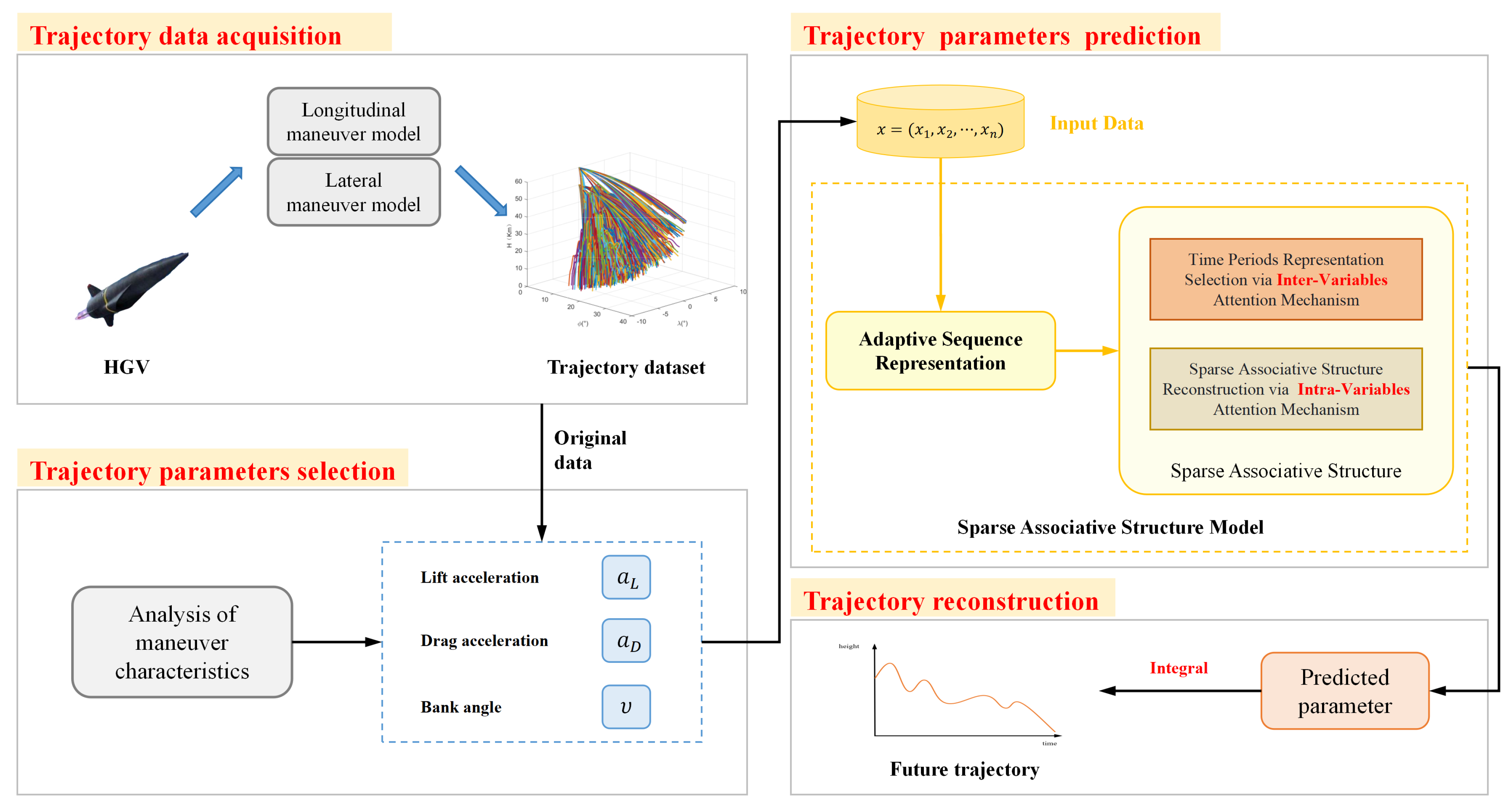
Figure 6 shows the framework of the HGV trajectory prediction model proposed in this paper, consisting of a trajectory data preprocessing module, a trajectory parameters selection module, a parameter prediction module, and a trajectory reconstruction module.
Initially, we constructed an extensive dataset of flight trajectories across various maneuvering modes, utilizing the methodology outlined in Section 2. Following this, an in-depth analysis of the maneuver characteristics led us to select three pivotal trajectory parameters, as Section 3.2 shows. We then input the original trajectory data into a prediction model that employs the SASM algorithm, as Section 4.1 devised. This model leverages an adaptive representation to encode the data sequences. By incorporating an attention mechanism, the model adeptly uncovers the sparse associative structures within the data, both among intravariable and intervariable relationships. These identified structures are subsequently integrated into the predictive network, which is tasked with forecasting the parameters. Ultimately, the forecasted parameters, in conjunction with the current states and motion Equations (1) of the HGV, are deployed to facilitate the reconstruction of the trajectory.

5. Simulation

In this section, we carry out simulation experiments to verify the effectiveness of the algorithm.

5.1. Sample Settings and Parameter Settings

(1)
Simulation Condition
The simulation analysis in this paper is conducted in the Python environment, and we utilize the Pytorch framework to construct the network. The hardware is configured with an Interi7 processor and a gegforce 2060 graphics card.
(2)
Trajectory Dataset Setting
During the training phase, we generate 15,000 HGV trajectories based on the trajectory generation method mentioned in Section 2.3. The initial state parameters setting and control parameters setting of the HGV are shown in Table 2 and Table 3, respectively. The explanations of the state parameters and control parameters are shown in Section 2.1 and Section 2.2. Random flight trajectories of the HGV can be obtained by randomly selecting and combining the values of the initial state parameters and the related parameters of control variables. Therefore, each trajectory in the dataset is distinct. The trajectory dataset of the HGV is shown in Figure 7.
(3)
Training setting
During model training, we used the adaptive moment estimation (Adam) optimizer and L2 loss function. The parameters of the Adam optimizer and the SASM are shown in Table 4.
During the training phase, 80% of the data were used for model training, 10% for validation data, and 10% for testing data.
Meanwhile, in order to objectively evaluate the performance of the proposed model in this paper, two indicators were adopted here to measure the prediction error, namely, the Mean Square Error (MSE) and the Mean Absolute Error (MAE), with the corresponding formulas as follows:
e MSE = 1 N i = 1 N ( a ^ a ) 2
e MAE = 1 N i = 1 N a ^ a
where a ^ and a are the parameters predicted by the SASM and the true value, respectively.
We also calculated the average error of spatial distance (AESD) of the trajectory prediction error with the following formula:
AESD = 1 N i N k L p 1 L p X p k i X l k i 2 + Y p k i Y t k i 2 + Z p k i Z t k i 2
where L p is the length of predicted time series, and [ X p k i , Y p k i , Z p k i ] indicates the location of ith test data and true data in the three dimensions of longitude, latitude, and height predicted at k time, respectively.
What is more, we compared the model’s transfer ability from known data to unknown data in order to validate the model’s generalization ability. We used different sources of data for the training model and the final test model, namely, the sources of data came from different types of HGVs. The inherent parameters (mass, cross section, etc.) of different kinds of vehicles are different, leading to their different flight paths, even under the same initial conditions. Specifically, we conducted verification experiments on three sets of trajectories generated for three types of HGVs. The number of test sets for each of the three types was 250.

5.2. Presentation and Comparison of Experimental Results

To comprehensively evaluate the performance of our proposed SASM model, we engaged in a comparative analysis that contrasted the predictive results of our SASM model with those produced by a singular LSTM model, a GRU model, and a sophisticated CNN-LSTM model [27]. This comparative analysis delved into three crucial dimensions: the architecture and parameters of the models, the prediction errors of the parameters, and the comparison of trajectory prediction curves.

5.2.1. Architecture and Parameters of Models

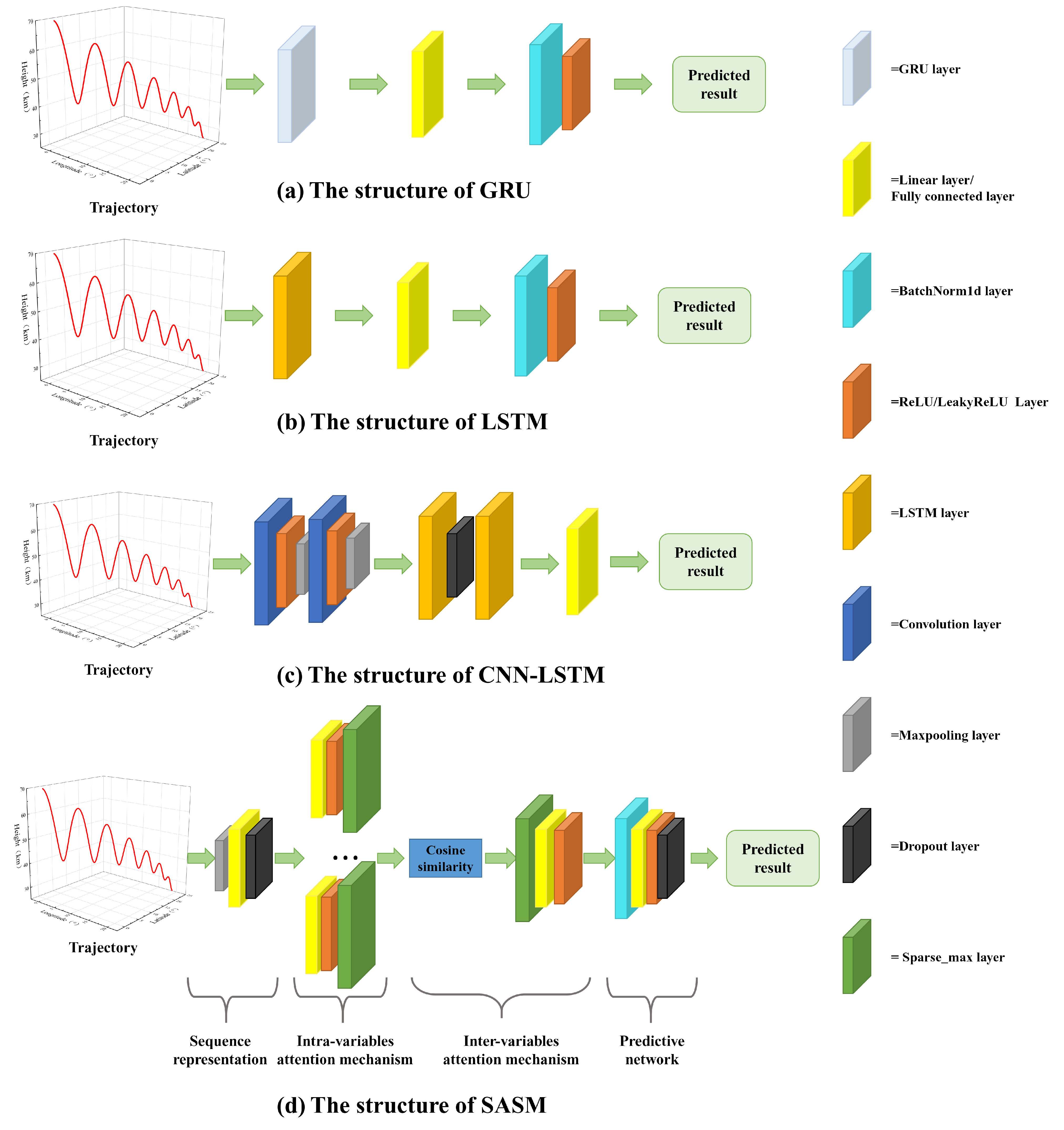
The different architectures of the above three models are depicted in Figure 8. The number of input features was 6 for each model.
The LSTM model includes a LSTM hidden layer, a linear layer, a 1D batch normalization layer, a ReLU activation layer, and a fully connected layer. The size of the hidden layer of the LSTM was set to 50. The number of kernels was set to 1 in the fully connected layer.
Compared to the LSTM, the GRU model simplifies the structure of the LSTM. There are only two gates in the GRU, namely, a reset gate and an update gate. The structure and parameters settings are consistent with the LSTM, except that the first layer is replaced with a GRU layer.
The CNN-LSTM model comprises two sections: a convolution part and an LSTM part. The convolution portion consists of two identical structures, with each featuring a convolution layer, a ReLU activation layer, and a max pooling layer. The LSTM section, on the other hand, includes two LSTM layers and a dropout layer. The two convolution layers contain 32 individual 1 × 3 convolution kernels each. The dropout rate of two dropout layers is 0.2. Its two LSTM layers both have 50 hidden nodes. The size of kernel is 1 in the final fully connected layer.
The SASM model, as devised in this paper, is structured into four components. Initially, the trajectory data are fed into the sequence representation module, which comprises an adaptive max pooling layer, an LSTM hidden layer, and a dropout layer. The adaptive length of the adaptive max pooling layer is 900. The LSTM has 10 hidden nodes, and the dropout rate is 0.2. Following separate processing through intravariable and intervariable attention mechanisms, the associative structural representation was obtained. The input and output feature dimensions of the attention network were both 10. Finally, this representation was input into the predictive network, from which future parameters were predicted. The predictive network was constructed with a 1D batch normalization layer, a linear layer, a ReLU activation layer, and a dropout layer. The size of the linear layer was set to 50.

5.2.2. Prediction Errors of Parameters

We examined three different types of HGVs (described as I, II, and III in Table 5) as the test data, where the prediction errors of parameters are illustrated in Table 5.
Based on Table 5, it is clear that the two evaluation metrics (MSE and MAE) of the SASM outperformed the LSTM, GRU and CNN-LSTM in predicting the parameters for each category of the HGV. Specifically, in the prediction of aerodynamic lift acceleration, the SASM method demonstrated a notable improvement, with the maximum MSE reduction rate reaching 22.56% and the maximum MAE reduction rate reaching 19.39%, both when contrasted with the LSTM method. The performance enhancement was further accentuated in the prediction of drag acceleration, where the reduction rates for the MSE and MAE were at their zenith, peaking at 35.31% and 31.28%, respectively, across the three types of test data. Most notably, the SASM model exhibited a significant leap in the precision of bank angle prediction. The maximum reduction rates for the MSE and MAE are strikingly high, at 93.86% and 73.29%, respectively. The SASM’s MSE values are a mere one-third of those produced by the CNN-LSTM and a tenth of those from the LSTM, underscoring the model’s exceptional predictive accuracy in this parameter.
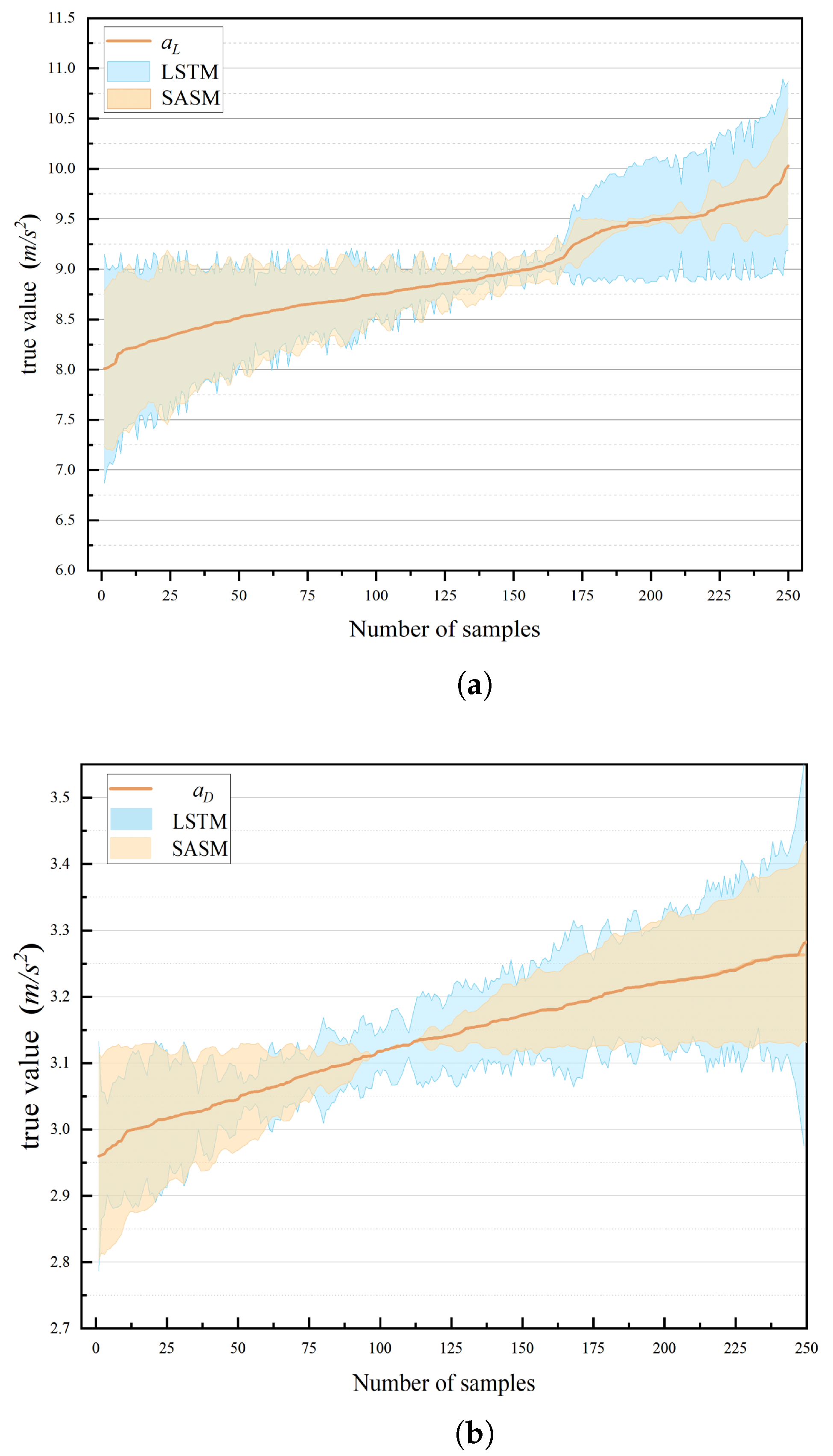
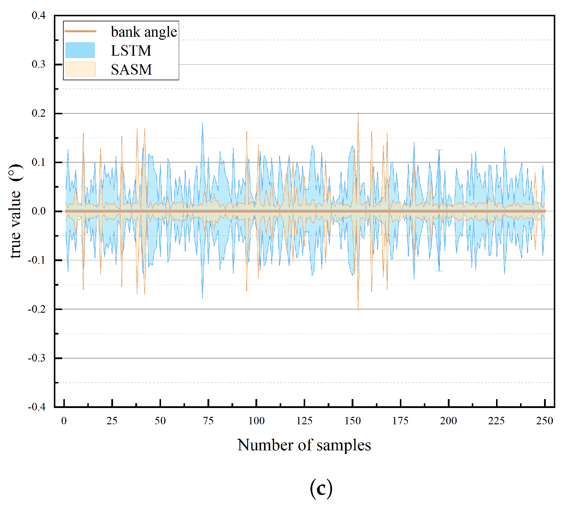
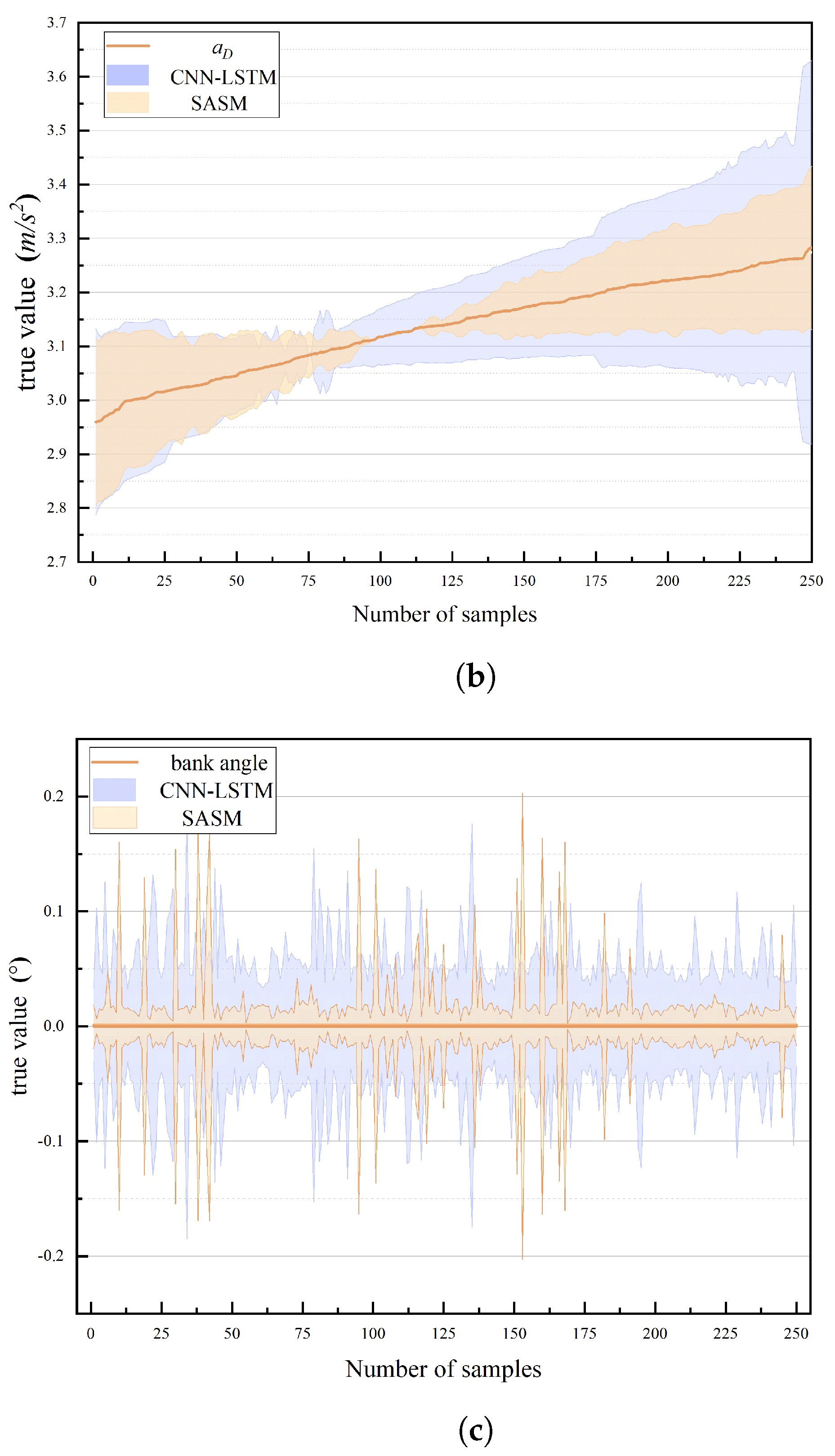
Furthermore, taking test data I as an example, we conducted a comparative analysis of the predictive performance between our proposed model and the LSTM model across various numerical ranges of parameters, as depicted in Figure 9. Figure 9a–c illustrate the error curve when predicting the aerodynamic lift acceleration a L , drag acceleration a D , and bank angle ν for the SASM and LSTM models, respectively. Initially, as shown in Figure 9a, the error bands of the two models are quite similar. However, as a L increased, the predictive error for both models decreased, reaching a nadir for the LSTM when a L equaled 9.25 m / s 2 . At this point, the LSTM’s error margin expanded noticeably, whereas the error for the SASM (represented by the orange area) is considerably smaller than that of the LSTM (the blue area). Furthermore, when a L reached 9.5 m / s 2 , the error for the SASM escalated at a more gradual pace compared to the LSTM. Figure 9b exhibits a pattern akin to that in Figure 9a, with the SASM model demonstrating superior predictive performance for the drag acceleration a D within the range of [3.1, 3.2] m / s 2 . Figure 9c demonstrates a notably smaller error band for the SASM model, compared to LSTM. While it is true that the LSTM model exhibited superior performance at certain, albeit rare, data points, the overall trend highlights the SASM model’s advantage in terms of consistency and precision in predictions.
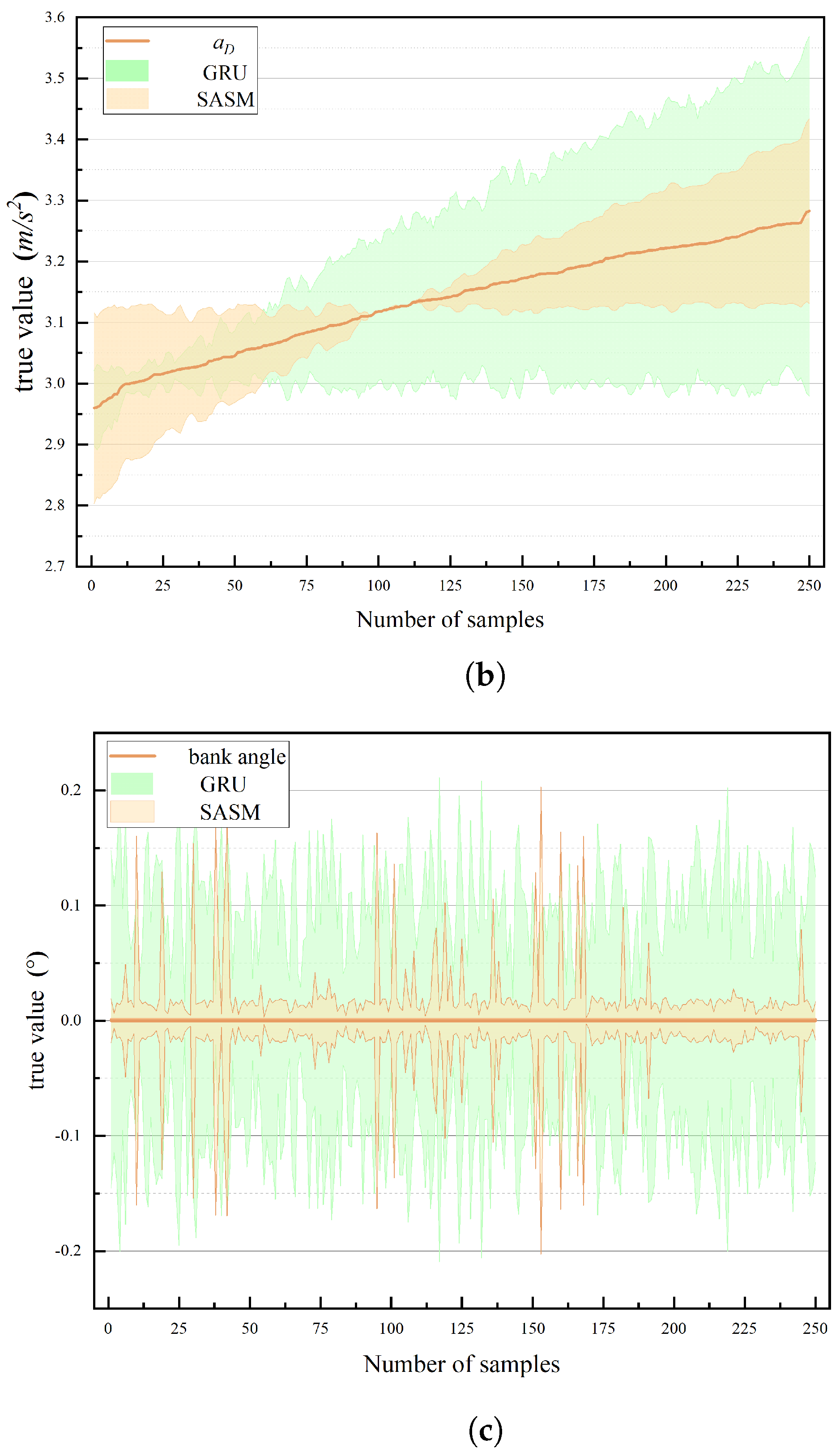
Additionally, Figure 10 presents a comparative analysis of the error between the SASM and CNN-LSTM models. In Figure 10a, prior to reaching 9.25 m / s 2 , the prediction errors for the aerodynamic lift acceleration a L were decreasing for both the SASM and GRU model. And their error bands are quite similar. Subsequently, the error bands expanded, with the GRU model exhibiting a more rapid and pronounced increase compared to the SASM model. Similarly, the trends observed in Figure 10b,c, mirror those seen in Figure 10a.
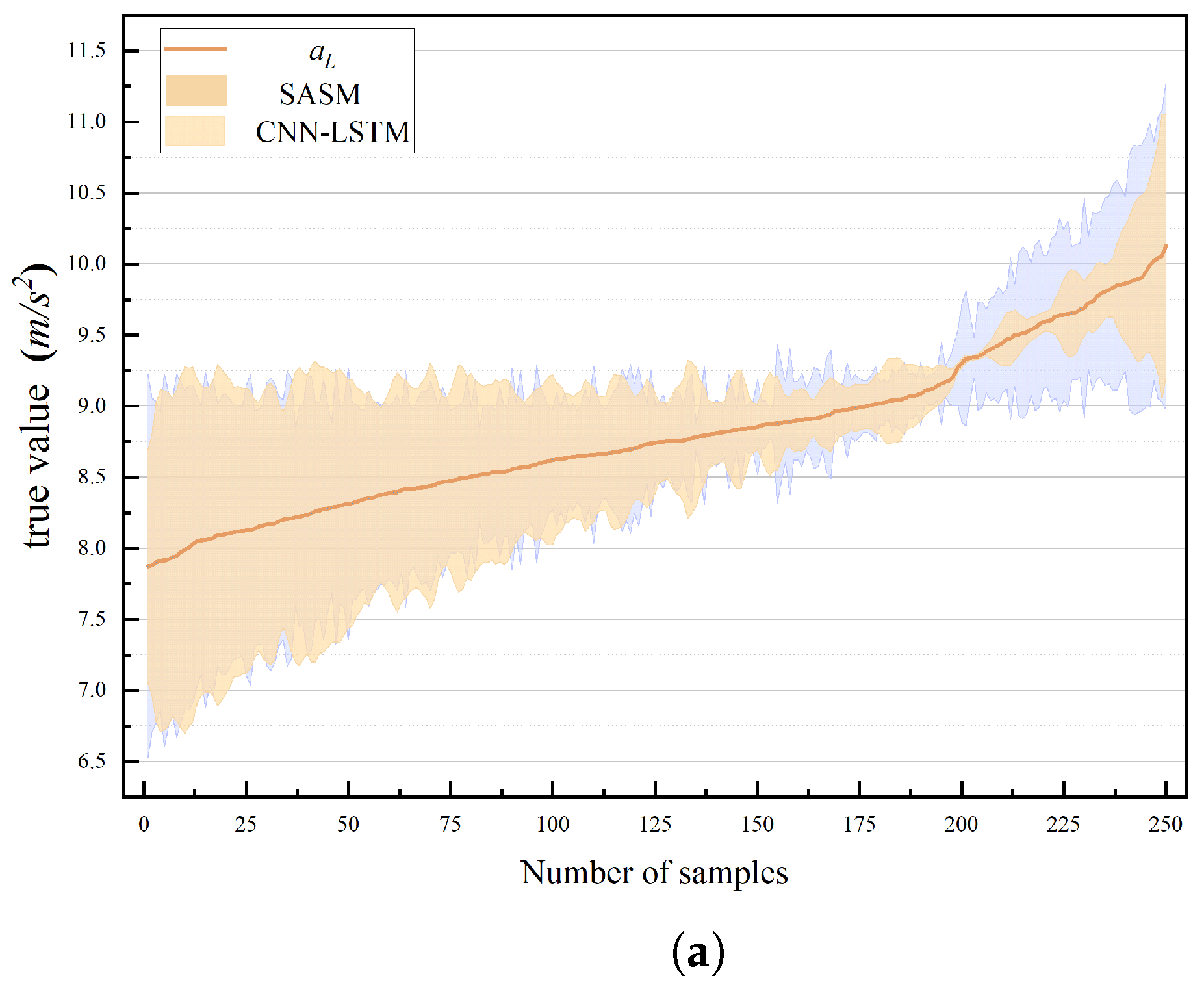
a L and a D error curves of CNN-LSTM model in Figure 11a are similar to the curves of GRU model, except that entire errors of GRU are smaller than CNN-LSTM. For error curve of ν , GRU model does not perform as well as CNN-LSTM model, as shown in Figure 11. In summary, the ranking of models based on prediction error is SASM < CNN-LSTM < GRU < LSTM, while the ranking based on prediction accuracy is the inverse: SASM > GRU > CNN-LSTM > LSTM.

5.3. Comparison of Trajectory Prediction Curves

The reconstructed trajectory of the HGV was generated utilizing the parameters forecasted by the SASM method and subsequently compared against the predictions of the LSTM, GRU, and CNN-LSTM method. The 100-step future trajectories of the HGV for each model are illustrated in Figure 12. Figure 12a presents a three-dimensional visualization of both the predicted and actual trajectories. Figure 12b depicts the two-dimensional plot of the predicted and actual trajectories in terms of latitude and height.
As can be seen from Figure 12a, the 3D predicted trajectories of all four models generally maintained the trend of the actual trajectory. Notably, the SASM method demonstrated the smallest error and superior predictive performance compared to other models. The projected values of the three methodologies onto the latitude and longitude coordinate axes demonstrated minimal deviation from the actual values, with the primary disparity manifesting in the height prediction, as Figure 12b shows. It is evident that the prediction based on the SASM was closest to the true trajectory and had the smallest error. The GRU followed closely, with the CNN-LSTM slightly behind the GRU, while the LSTM exhibited a more pronounced deviation from the actual trajectory compared to the other two models. Overall, the models’ predictive accuracy values are ranked as follows: SASM > GRU> CNN-LSTM > LSTM.
The AESD and average processing time of three models are detailed in Table 6. Notably, the SASM method exhibited the lowest AESD among the three, with a value of 0.049518. This represents a substantial 90.21% reduction in the AESD compared to the LSTM method. Furthermore, the average processing time of the SASM was also the shortest, clocking in at 7.790 (assuming the unit is appropriate for the context), which is approximately 49.7% faster than the LSTM method. These results underscore the efficiency and accuracy advantages of the SASM method over the LSTM method for the given application.

6. Results

This paper introduces a groundbreaking trajectory forecasting approach that integrates the Sparse Associative Structure Model (SASM) with deep learning and dynamic equations, addressing the longstanding challenges of accuracy and generalization in traditional methods. We applied the research of time domain adaptation to the field of theHGV, which has provided a new way to solve the field of the HGV.
Firstly, we constructed a comprehensive trajectory database that encompasses diverse maneuvering modes, laying a robust foundation for our predictive model. Subsequently, we identified three crucial trajectory parameters as prediction targets and devised a prediction model based on the SASM. Ultimately, this trained model was leveraged to anticipate the trajectory parameters of the HGV, enabling the reconstruction of their future trajectories for real-time prediction. In the simulation experiment, we compared the generalization performance of the models by comparing their prediction accuracy on different data sets. In particular, the test data sets and training data sets were derived from different types of aircraft. The simulation results show that the prediction accuracy of the SASM was superior to the LSTM, GRU, and CNN-LSTM models. Notably, the SASM reduced the trajectory prediction error by an impressive 50.35% and shortened the average processing time by 48.7% compared to the LSTM model. This proposed methodology has demonstrated remarkable proficiency in forecasting trajectories for three distinct types of HGVs, boasting both high prediction accuracy and excellent generalization capabilities.
However, the method proposed in this paper also has the following limitations: (1) The model is currently capable of short-term trajectory prediction for HGVs, with long-term predictions remaining a challenge. (2) Complex maneuver trajectories pose difficulties for accurate prediction. As such, future research endeavors should focus on advancing these aspects of trajectory prediction to further enhance their applicability and accuracy.

Author Contributions

Conceptualization, F.L. and L.L.; data curation, F.L. and Z.Z.; methodology, F.L. and L.L.; software, F.L. and Z.Z.; validation, F.L. and Z.Z.; formal analysis, L.L.; writing—original draft preparation, F.L.; writing—review and editing, L.L. and Y.X.; visualization, F.L. and Z.Z.; supervision, J.C. and Y.X.; funding acquisition, Y.X. All authors have read and agreed to the published version of the manuscript.

Funding

This work was supported in part by the National Natural Science Foundation of China (Grant Number 62173336 and 92271108).

Institutional Review Board Statement

Not applicable.

Informed Consent Statement

Not applicable.

Data Availability Statement

The data presented in this study are available upon request from the corresponding author.

DURC Statement

The current research is limited to the aircraft trajectory prediction, which is beneficial to the development of deep learning technology in aircraft trajectory prediction and does not pose a threat to public health or national security. The authors acknowledge the dual-use potential of the research involving a hypersonic gliding vehicle and confirm that all necessary precautions have been taken to prevent potential misuse. As an ethical responsibility, the authors strictly adhere to relevant national and international laws regarding DURC projects. The authors advocate for responsible deployment, ethical considerations, regulatory compliance, and transparent reporting to mitigate misuse risks and foster beneficial outcomes.

Conflicts of Interest

The authors declare that they have no known competing financial interests or personal relationships that could have appeared to influence the work reported in this paper.

Correction Statement

This article has been republished with a minor correction to the DURC Statement. This change does not affect the scientific content of the article.

Appendix A. Explanation of Parameters

In the Appendix, we explain the terminologies about the angle in Equation (1) in Section 2.1, as shown in Table A1.
Table A1. Explanation of parameters.
SymbolParameterExplanation
θ Flight path angleAngle between the aircraft’s flight path vector and the local horizontal plane
σ Heading angleAngle between the aircraft’s longitudinal axis and true north axis in the horizontal plane
α Angle of attackAngle between the aircraft’s axis and the relative wind direction
ν Bank angleAngle between the aircraft’s wings and the horizontal plane
λ LongitudeDihedral angle between meridian plane and prime meridian plane
ϕ LatitudeLine between the aircraft and the Earth’s center and the line–plane angle of the Earth’s equator

References

  1. Zhao, L.; Yong, E.; Wang, B. Some achievements on interception of near space Hypersonic vehicles. J. Astronaut. 2020, 10, 1239–1250. [Google Scholar]
  2. Liu, S.; Yan, B.; Huang, W.; Zhang, X.; Yan, J. Current status and prospects of terminal guidance laws for intercepting hypersonic vehicles in near space: A review. J. Zhejiang-Univ.-Sci. 2023, 5, 387–403. [Google Scholar] [CrossRef]
  3. Cui, Y.; Xiong, W.; He, Y. Adaptive forecast model for uncertain trajectory tracking. Acta Aeronaut. Astronaut. Sin. 2019, 40, 322557. [Google Scholar]
  4. Zeng, W.; Quan, Z.; Zhao, Z.; Xie, C.; Lu, X. A Deep Learning Approach for Aircraft Trajectory Prediction in Terminal Airspace. J. Astronaut. 2020, 8, 151250–151266. [Google Scholar] [CrossRef]
  5. Liu, X.; Zhong, W.; Wang, X.; Duan, H.; Fan, Z.; Jin, H.; Huang, Y.; Lin, Z. Deep Reinforcement Learning-Based 3D Trajectory Planning for Cellular Connected UAV. Drones 2024, 8, 199. [Google Scholar] [CrossRef]
  6. Zhang, Y.; Wen, J.; Yang, G.; He, Z.; Luo, X. Air-to-Air Path Loss Prediction Based on Machine Learning Methods in Urban Environments. Wirel. Commun. Mob. Comput. 2018, 2018, 1–9. [Google Scholar] [CrossRef]
  7. Wu, K.; Pan, W. 4-D trajectory prediction model based on data mining. Comput. Appl. 2007, 27, 2637–2639. [Google Scholar]
  8. Zhang, H.; Xie, Y.; Chen, K.; Tang, G. Investigation on Trajectory Prediction of Maneuverable Target. Mod. Def. Technol. 2011, 6, 26–31. [Google Scholar]
  9. Wang, X.; Qin, W.; Bai, Y.; Cui, N. Trajectory estimation for ballistic missile in boost stage using robust filtering. IET Radar Sonar Navig. 2017, 3, 513–519. [Google Scholar] [CrossRef]
  10. Ji, R.; Liang, Y.; Xu, L.; Wei, Z. Trajectory prediction of ballistic missiles using Gaussian process error model. Chin. J. Aeronaut. 2022, 1, 458–469. [Google Scholar] [CrossRef]
  11. Zhou, J. Trajectory prediction method based on three-step numerical integration. Foreign Electron. Meas. Technol. 2017, 36, 13–16. [Google Scholar]
  12. Wu, H.; Cha, Q.; Liang, S.; Zhang, S. Research on Ballistic Trajectory Extrapolation Method Based on Genetic Algorithm. Command. Control. Simul. 2021, 5, 102–106. [Google Scholar]
  13. Moon, C.; Song, K.; Kim, S.; Choi, H. State Prediction of High-speed Ballistic Vehicles with Gaussian Process. Int. J. Control. Autom. Syst. 2018, 16, 1282–1292. [Google Scholar] [CrossRef]
  14. Fan, P.; Guo, Y.; Fan, Y.; Yan, J. Footprint Calculation of HGV with Equilibrium Gliding Trajectory. Comput. Meas. Control. 2019, 27, 136–140. [Google Scholar]
  15. Wang, K.; Xu, Z.; Tang, S.; Wan, J. A Trajectory Prediction Method for Near Space Short-range Glide Vehicle Based on Flight Mission. J. Astronaut. 2021, 42, 50–60. [Google Scholar] [CrossRef]
  16. Wang, Q.; Ran, M.; Zhao, Y. Reentry guidance for hypersonic vehicle based on predictor-corrector method. J. Beijing Univ. Aeronaut. Astronaut. 2013, 12, 1563–1567. [Google Scholar]
  17. Li, G.; Zhang, H.; Tang, G. Typical Trajectory Characteristics of Hypersonic Glide Vehicle. J. Astronaut. 2015, 4, 397–403. [Google Scholar]
  18. Li, J.; Guo, J.; Tang, S. Trajectory Prediction Based on Multi-model and Multi-intent Fusion for Hypersonic Gliding Targets. J. Astronaut. 2024, 2, 167–180. [Google Scholar]
  19. Wang, L.; Xing, Q.; Mao, Y. Trajectory prediction of reentry hypersonic glide vehicle based on changing rule of lift-drag ratio. Syst. Eng. Electron. 2015, 10, 2335–2340. [Google Scholar]
  20. Zhai, D.; Lei, H.; Li, J.; Liu, T. Trajectory prediction of hypersonic vehicle based on adaptive IMM. Acta Aeronaut. Astronaut. Sin. 2016, 11, 3466–3475. [Google Scholar]
  21. Zhang, J.; Xiong, J.; Lan, X.; Xi, Q.; Xia, L.; Zhang, K. An Intelligent Prediction Method of Hypersonic Glide Vehicle Trajectory. J. Astronaut. 2022, 4, 413–422. [Google Scholar]
  22. Cai, R.; Chen, J.; Li, Z.; Chen, W.; Zhang, K.; Ye, J.; Li, Z.; Yang, X.; Zhang, Z. Time Series Domain Adaptation via Sparse Associative Structure Alignment. In Proceedings of the AAAI Conference on Artificial Intelligence(AAAI), Online, 2–9 February 2021. [Google Scholar]
  23. Zhang, J.; Xiong, J.; Li, L.; Xi, Q.; Chen, X.; Li, F. Motion State Recognition and Trajectory Prediction of Hypersonic Glide Vehicle Based on Deep Learning. IEEE Access 2022, 10, 21095–21108. [Google Scholar] [CrossRef]
  24. Yong, E.; Tang, G.; Chen, L. Rapid Trajectory Optimization for Hypersonic Reentry Vehicle Via Gauss Pseudospectral Method. J. Astronaut. 2008, 6, 1766–1772. [Google Scholar]
  25. Li, X.; Jilkov, V.P. Survey of Maneuvering Target Tracking. Part II: Motion Models of Ballistic and Space Targets. IEEE Trans. Aerosp. Electron. Syst. 2010, 46, 96–119. [Google Scholar] [CrossRef]
  26. Martins, A.; Astudillo, R. From Softmax to Sparsemax: A Sparse Model of Attention and Multi-Label Classification. In Proceedings of the 33rd International Conference on International Conference on Machine Learning, New York, NY, USA, 19–24 June 2016. [Google Scholar]
  27. Ma, L.; Shan, T. A hybrid cnn-lstm model for aircraft 4d trajectory prediction. IEEE Access 2020, 8, 134668–134680. [Google Scholar] [CrossRef]
Figure 1. Process of trajectory generation.
Drones 08 00505 g001
Figure 2. Process of trajectory generation.
Drones 08 00505 g002
Figure 3. Trajectories of longitudinal maneuvers. (a) Balanced gliding state. (b) Jumping gliding state.
Drones 08 00505 g003
Figure 4. The change law of aerodynamic lift acceleration. The red line denotes height, while the blue is lift acceleration.
Drones 08 00505 g004
Figure 5. The structure of SASM.
Drones 08 00505 g005
Figure 6. Framework of trajectory prediction model.
Drones 08 00505 g006
Figure 7. Trajectory dataset of HGV.
Drones 08 00505 g007
Figure 8. Architecture of different models.
Drones 08 00505 g008
Figure 9. Error curve comparison between SASM and LSTM. (a) Perdition of lift acceleration. (b) Perdition of drag acceleration. (c) Perdition of bank angle.
Drones 08 00505 g009aDrones 08 00505 g009b
Figure 10. Error Curve Comparison between SASM and GRU. (a) Perdition of lift acceleration; (b) Perdition of drag acceleration; (c) Perdition of bank angle.
Drones 08 00505 g010aDrones 08 00505 g010b
Figure 11. Error curve comparison between SASM and CNN-LSTM. (a) Perdition of lift acceleration. (b) Perdition of drag acceleration. (c) Perdition of bank angle.
Drones 08 00505 g011aDrones 08 00505 g011b
Figure 12. Trajectoryprediction curves of different models. (a) 3D trajectory prediction curves. (b) 2D trajectory prediction curves.
Drones 08 00505 g012
Table 1. Pseudo-code of trajectory parameters prediction based on SASM.
Trajectory Parameters Prediction Algorithm Based on SASM
Input: λ , ϕ , r, V, θ , σ of HGV, labels of trajectory parameter.
Output: Predicted trajectory parameters.
   1: Identification of candidate time period x i ˜ .
   2: Representation of the candidate time periods based on Equation (8).
   3: Calculate weight α i of each time period via intra-variables attention mechanism by Equations (10) and (11).
   4: Get the weighted time period representation Z i based on Equation (12).
   5: Calculate the associative weight β i between time periods via inter-variables attention mechanism according to Equation (14).
   6: Get the associative structure representation U i based on Equation (15).
   7: Get the final representation H i based on Equation (16).
   8: Get the predictive result y p r e based on Equation (17).
Table 2. Initial state parameters setting of HGV.
ParameterRange of ValueUnit of Value
H 0 50, 60kilometer (km)
V 0 [7, 15] *Mach (Ma)
λ 0 , ϕ 0 0degree (∘)
θ 0 −0.5, 0, 0.5degree (∘)
ψ 0 45degree (∘)
represents a number that randomly takes the range.
Table 3. Control parameters setting of HGV.
ParameterRange of ValueUnit of Value
V 1 [1250, 1500] *meter/second (m/s)
V 2 [3000, 4000] *meter/second (m/s)
α max [15, 25] *degree (°)
α K [10, 15] *degree (°)
ν 0 0degree (°)
ν max [25, 55] *degree (°)
N0, 1, 2/
f−1, 1/
T M o v i n g n [ 80 ± 40 , 250 ± 80 ] , [ 400 ± 50 , 620 ± 100 ] *second (s)
represents a number that randomly takes the range.
Table 4. Training parameters settings of optimizer.
TypeParameterRange of Value
Adam optimizerlearning rate0.001
weight decay 1 × 10 5
adjustment rate of learning rate0.3
batch size1024
Parameters in SASM algorithmhidden dimension10
dense dimension50
probability of drop layer0.01
number of candidate period4
Table 5. Comparision of prediction error of different models.
Type of DataParameterModelMSEMAE
I a L LSTM0.6118920.697823
CNN-LSTM0.5356540.62998
GRU0.5007310.590700
SASM0.473891 (22.56%)0.562499 (19.39%)
a D LSTM0.1433130.290542
CNN-LSTM0.1858610.297423
GRU0.1393450.295436
SASM0.122914 (35.31%)0.273727 (31.28%)
ν LSTM0.0229070.124759
CNN-LSTM0.0058890.070541
GRU0.0174290.123651
SASM0.005441 (76.25%)0.042601 (65.85%)
II a L LSTM0.5423480.603019
CNN-LSTM0.4957630.589409
GRU0.4769610.558551
SASM0.460275 (15.13%)0.543206 (9.92%)
a D LSTM0.1986620.380969
CNN-LSTM0.1487520.332633
GRU0.1426730.320038
SASM0.125630 (36.76%)0.299648 (21.35%)
ν LSTM0.0145870.099969
CNN-LSTM0.0035710.058099
GRU0.0139330.113739
SASM0.000896 (93.86%)0.026697 (73.29%)
III a L LSTM1.0672040.806777
CNN-LSTM0.9244360.770901
GRU0.8858220.747409
SASM0.865717 (18.88%)0.736459 (8.72%)
a D LSTM0.2211090.346958
CNN-LSTM0.1776270.297109
GRU0.1806930.302941
SASM0.160217 (27.54%)0.279107(19.56%)
ν LSTM0.0149560.102023
CNN-LSTM0.0035280.058556
GRU0.0026210.034570
SASM0.000971(93.51%)0.028235 (72.32%)
(%) indicates the reduction compared with LSTM method for the proposed approach.
Table 6. Comparision of model in AESD and average processing time.
ModelAESD/kmTime/s
LSTM0.50183715.487
CNN-LSTM0.34149711.105
GRU0.28563711.926071
SASM0.249158 (50.35%)7.790 (49.70%)
Disclaimer/Publisher’s Note: The statements, opinions and data contained in all publications are solely those of the individual author(s) and contributor(s) and not of MDPI and/or the editor(s). MDPI and/or the editor(s) disclaim responsibility for any injury to people or property resulting from any ideas, methods, instructions or products referred to in the content.