Hyperspectral Sensor Management for UAS: Performance Analysis of Context-Based System Architectures for Camouflage and UXO Anomaly Detection Workflows

Abstract

Tactical aerial reconnaissance missions using small unmanned aerial systems (UASs) have become a common scenario in the military. In particular, the detection of visually obscured objects such as camouflage materials and unexploded ordnance (UXO) is of great interest. Hyperspectral sensors, which provide detailed spectral information beyond the visible spectrum, are highly suitable for this type of reconnaissance mission. However, the additional spectral information places higher demands on system architectures to achieve efficient and robust data processing and object detection. To overcome these challenges, the concept of data reduction by band selection is introduced. In this paper, a specialized and robust concept of context-based hyperspectral sensor management with an implemented methodology of band selection for small and challenging UXO and camouflaged material detection is presented and evaluated with two hyperspectral datasets. For this purpose, several anomaly detectors such as LRX, NCC, HDBSCAN, and bandpass filters are introduced as part of the detection workflows and tested together with the sensor management in different system architectures. The results demonstrate how sensor management can significantly improve the detection performance for UXO compared to using all sensor bands or statistically selected bands. Furthermore, the implemented detection workflows and architectures yield strong performance results and improve the anomaly detection accuracy significantly compared to common approaches of processing hyperspectral images with a single, specialized anomaly detector.

1. Introduction

The operation of spectral sensors on UASs has become increasingly important and representative in current research. In particular, hyperspectral sensor technology has made significant progress in the last recent years, resulting in smaller and more cost-effective sensors [1]. These technological advances allow effective operation on a UAS, enabling flexible and rapid deployment of hyperspectral sensors over long distances and large areas [2,3,4,5,6]. In addition, hyperspectral sensors provide rich spectral information beyond the visual spectrum and therefore high spectral differentiability, providing great advantages in detecting visually obscured or small objects in challenging environments, such as camouflage materials and UXO [7,8,9,10]. This flexibility and rapid deployment, combined with long-range capability and rich spectral information, make hyperspectral sensors on tactical drones highly suitable for the UXO and camouflage tactical reconnaissance missions considered here. However, a sensor operation on a UAS is limited by the maximum payload weight, onboard computing, and link capacities for in-mission data exchange [11,12]. This, combined with the high spectral information density and the resulting high data rate, makes hyperspectral sensors challenging to deploy. The varying information content of spectral sensor bands, depending on the target and environment, also poses significant challenges for targeted data processing or data compression to overcome these limitations [12,13,14,15]. Therefore, the Band Selection (BS) methodology was introduced to achieve data reduction and also a higher detection performance through the systematic task-oriented selection of spectral sensor bands before further processing like object detection.

There are several approaches for object detection on spectral images [8,16,17]. According to [18,19], a distinction can be made between anomaly detection, which relies on anomalous spectral pixels in the image, and signature-based target detection, which relies on previously known spectral signatures of the targets and/or the environment. Methods such as matched filtering or spectral unmixing combined with endmember extraction are based on the latter approach. Instead of searching for targets based on their anomalies relative to the data, the approach attempts to distinguish the known spectral signature of the target from that of the target’s environment and make a decision about the likelihood of positive target detection based on the totality of the extracted signatures. However, this is where the biggest challenge lies [20,21,22,23,24,25,26,27,28,29,30,31,32]: On the one hand, signatures must be known very precisely to achieve a sufficient level of detectability even under non-ideal conditions. This need extends not only to target signatures but also to other critical information. For procedures such as endmember extraction, the exact number of additional material signatures must also be known, which is often not the case for the use case discussed in this paper. In addition, the material signatures in the hyperspectral images (HSIs) are not available in pure form. Due to the spatial resolution of HSIs, image pixels often capture multiple materials within a single pixel. As a result, individual pixel values can represent a mixture of multiple spectral signatures, requiring the separation of these mixed signatures. While methods such as spectral unmixing exist to address these challenges, they often struggle with small targets and require significant computing resources, making object detection difficult. Other factors, such as viewing angle or lighting conditions, pose additional challenges in accurately processing target spectral signatures to achieve reliable target detection. Therefore, object detection based on known spectral signatures is less suitable for reconnaissance missions that involve complex and partially unknown environments, lack of target signatures, changing environmental conditions, and the detection of small objects such as UXO. Such missions require robust detection methods capable of operating under changing, difficult, and unknown conditions.

The anomaly detection approach, on the other hand, focuses on identifying anomalous pixels in a dataset, such as a unique small mine in a field. To identify these anomalous pixels, each hyperspectral image pixel is compared to its neighboring image pixels to assess its uniqueness [33,34]. The advantages of anomaly detection can be derived from this approach. By searching for the anomaly in the dataset instead of a specific signature, no prior specific knowledge of the target signature or its environment is required. Thus, the detectability of targets is not limited to known targets and further prior knowledge [35,36]. In particular, it can effectively handle challenging unknown targets with variable textures and appearances, such as camouflage materials and UXO, due to their distinctiveness compared to the surrounding environment. This detection approach is therefore very suitable for the use case of challenging airborne tactical reconnaissance missions for UXO and camouflage detection. Hence, this paper focuses on a specialized BS for object detection through anomaly detection. For this purpose, the nature of such algorithms requires that the bands selected by the BS provide the greatest differentiation between the target and its environment [37]. The selection of the spectral bands and their differentiability of the target and the environment, here often denoted as sensor performance, depends on the targets and the environment themselves. Both target and environment are driven by the prior defined reconnaissance mission task and the actual image scene captured by the sensor, denoted as sensor context. This also applies for the detection performance of anomaly detectors [6]. Again, the mission task and sensor context will cause the anomaly detection performance to vary, as will the detector itself and its parameter settings too. At the same time, the detector performance also depends on the selected spectral image bands with their specific and sensor context-dependent information, which are the input of the detector. These relationships between mission task, sensor context, sensor performance, band selection, and anomaly detectors has hardly been studied yet and are often neglected in the development of architectural system designs for hyperspectral image processing.

Therefore, this paper analyzes this conditionality to derive improved processing architectures and anomaly detection performances. To achieve this, a range of studies are conducted within this paper. On the one hand, the benefits of the described context knowledge for BS are analyzed. For this purpose, the approach of Sensor Management with an integrated dynamic and context-based BS, specialized for anomaly detection of UXO and camouflage materials, is presented, evaluated, and compared to a statistical BS without the use of contextual mission knowledge, as well as to the processing of the full hyperspectral band set. The introduced Sensor Management is characterized by a targeted and automated prediction of sensor performance, taking into account the specific mission task and the mission environment, resulting in a robust and effective reduction of information and computing power while improving anomaly detection without the need of specific spectral target knowledge. This can also be considered innovative, as the authors are not aware of any hyperspectral sensor management system to date. In the field of spectral sensor management, there is one similar management system presented by [38,39]. This system focuses on multispectral sensor management for camouflage detection. This means that neither the challenging UXO detection nor the characteristics of the significantly higher information content of hyperspectral data are taken into account by this sensor management system and are therefore not comparable. On the other hand, the achievements for a targeted use of mission task-oriented and sensor context-based anomaly detectors and their parameter settings under consideration of the provided and extracted context knowledge are evaluated. Then, the BS and the anomaly detection are considered together and analyzed for their interferences. The aim is to determine the influence of combining various architectures and their interconnections of the Sensor Management’s BS and anomaly detectors on the overall anomaly detection performance. Through the systematic analysis of the relationships in this paper, the recommendations and the introduced system architectures with their use of contextual knowledge can achieve improved anomaly detection performance. For this purpose, unsupervised and training-free anomaly detectors are used. One of the best known anomaly detection algorithms is the Reed–Xialoi detector (RXD), which is further developed in its various variants [40,41,42]. One of the main advantages of RXD is that it requires little or no knowledge of the targets being searched for [42,43]. Thus, the RXD belongs to the group of unsupervised, statistic-based anomaly detectors. Only the approximate target size should be known in order to determine the areas to compare for an anomaly, which is often the case even in reconnaissance tasks. This makes the RXD a benchmark in hyperspectral image processing, which is often characterized by little available training data [42,44]. Although the availability of hyperspectral images for the use of training data has improved significantly, there are still crucial challenges [45]. On the one hand, most of the available HSI data are satellite-based or generated by high-altitude aircraft, as can be seen in [44], which lists some of the best-known HSI databases. Due to the presence of spectral targets in the HSI and the low spatial resolution, these data are not suitable for tactical reconnaissance applications. In particular, for targets with very limited information, such as camouflage materials or UXO, the generation of a training dataset is very challenging, especially with respect to the addition of new, previously unknown targets [46]. On the other hand, labeling the HSI to generate training data is challenging, and it is difficult to achieve generalization of the models trained with it [45]. The use of supervised and semi-supervised anomaly detectors, such as CNN- or Autoencoder-based detectors, with the need of training with HSI is therefore not suitable for the application of reconnaissance tasks that require robust detection and classification even for unknown targets in unknown environments. Instead, this work focuses on unsupervised and training-free anomaly detectors, such as the RXD, and investigates how to improve detection performance while maintaining the advantage of generalizability by selecting different targeted unsupervised anomaly detectors based on the sensor context without target knowledge. In addition to RXD, other detection methods such as a clustering-based method using Hierarchical Density-Based Spatial Clustering of Applications with Noise (HDBSCAN), a bandpass filter, and an anomaly method using Normalized Cross Correlation (NormXCorr) are used. These detectors, which are based on a wide variety of approaches, are then used to study the behavior of the detectors with respect to different selected spectral bands as inputs. By varying the selection of the bands depending on the target group and the sensor context, it can be determined which selection criteria should be used for the selection of the detectors and the bands in order to have an optimal detection result. The contribution of this work can be summarized as follows:

• Introduction of a hyperspectral Sensor Management scheme that provides fast and targeted band selection for aerial reconnaissance missions for camouflage and UXO detection based on [37]. As a result of this carefully designed management scheme, significantly higher anomaly detection performance can be achieved, even in varying mission areas with spectrally unknown targets, with a significantly reduced processing time. Only through the specific scheme design for the use case of tactical reconnaissance missions for camouflage and UXO detection a short and on-board processing capability can be ensured while achieving high anomaly detection performance in challenging environments and with unknown targets.
• Introduction of a hyperspectral detection processing workflow for UXO and camouflage materials. The explicitly designed workflow based on use cases provides computational resources that minimize hyperspectral data processing while enabling high anomaly detection performance. This is made possible by the targeted implementation of different anomaly detector approaches, targeted downsampling, and processing of contour information. All this can be achieved by the specific workflows while keeping computational costs low to provide the capability for fast on-board computing, one of the key points in tactical aerial reconnaissance tasks.
• Investigation of the correlation between hyperspectral sensor management and hyperspectral detection workflows with architectural design recommendations to achieve maximum, robust, high anomaly detection performance with low computational requirements for variable reconnaissance missions, taking into account the mission context and lack of target knowledge.

2. Materials and Methods

In this section, the HSI datasets used to evaluate the results will be briefly introduced, followed by the Sensor Management scheme. Within the Sensor Management, the initial spectral data are reduced by BS to the meaningful bands with the expected highest target information. These spectrally reduced data are the input for the anomaly detectors, which are described and explained afterwards. Finally, the parameter configurations of the detectors for the two target groups of interest, the camouflage materials and the UXO, are defined by two workflows in Section 2.5.

2.1. HSI Datasets

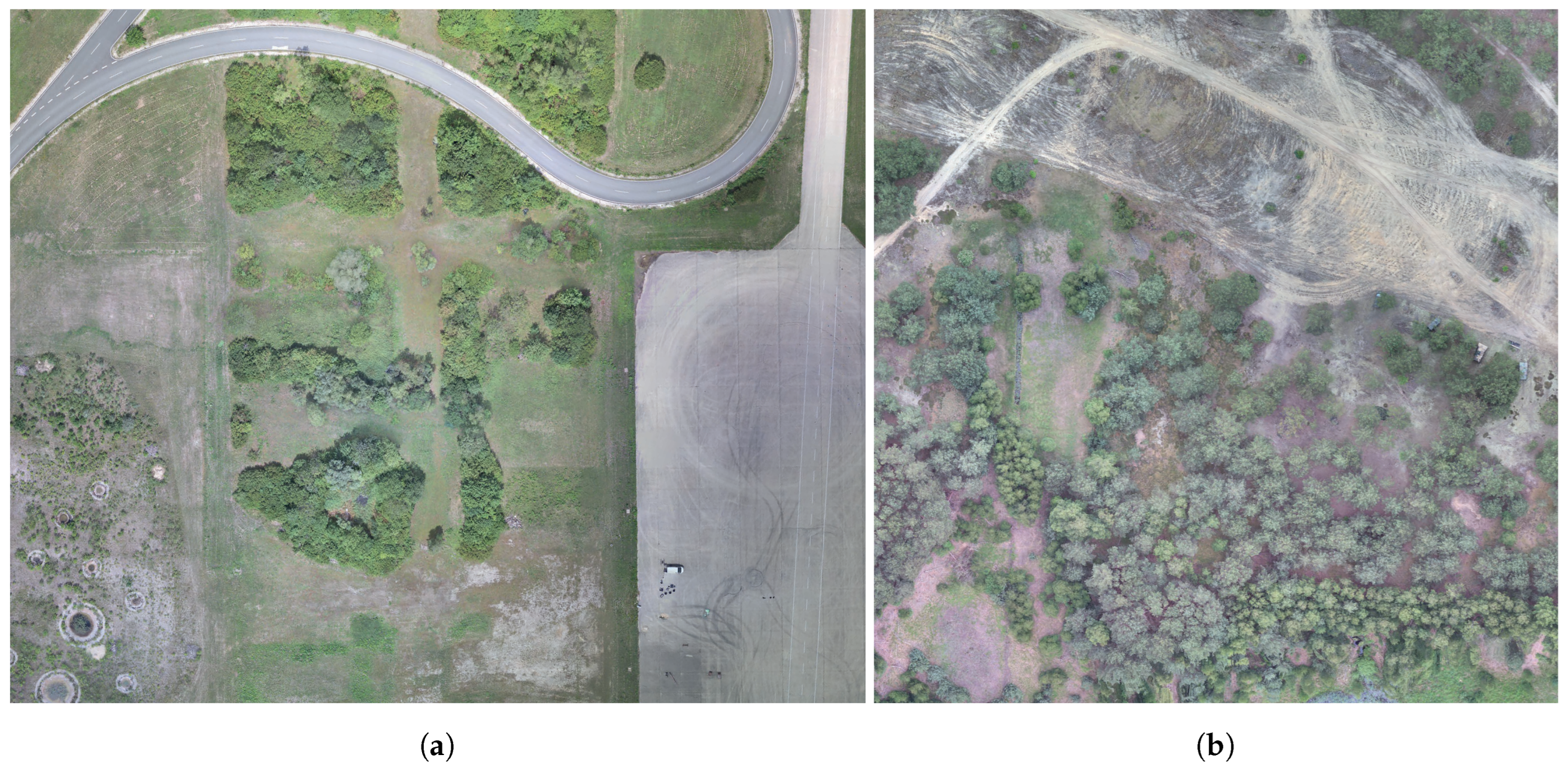
The HSI data consist of two different HSI datasets. These two datasets correspond to the datasets of [37], a previous publication of the authors, where further details and target configurations are described. Both datasets have the same ground sampling distance (GSD) of 0.065 m and cover a spectral range from 900 nm to 1700 nm with a spectral resolution of 8 nm and 224 spectral bands. All data were acquired with the hyperspectral camera Specim AFX17 at an altitude of 60 m, Nadir mounted in a M$\overline{o}$vi Pro gimbal on Freefly’s Alta X during varying seasons and times of day. As mentioned previously, two target groups, camouflage materials and UXO, are of particular interest and are represented in the datasets. Figure 1 shows some targets and their experimental setup on the ground that are included in both datasets. In total, dataset 1 contains 886 uncorrected atmospheric Nadir samples of 550 × 550 pixels and 356 depictions of 7 different UXO dummies and 790 depictions of 8 different camouflage materials. This includes 399 depictions of military-based camouflage materials such as the examples in Figure 1b–d and 391 depictions of improvised camouflage materials such as the tarp in the example in Figure 1a. The target representations differ in the location and illumination of the targets as well as in the seasons of winter, spring, summer, and fall when the HSI were taken. The whole dataset 1 was taken on testsite 1 in Figure 2a, which is characterized by a typical Central European landscape with meadow, deciduous forest, gravel, sand, and roads.

In contrast, dataset 2 contains samples of landscape with coniferous forest, swamp, moss, and sand, see Figure 2b. Overall dataset 2 includes 153 atmospheric uncorrected Nadir samples with 550 × 550 pixels and 102 depictions of the same 7 different UXO of dataset 1 and 239 depictions of camouflage materials, while 22 depictions are of the 4 improvised camouflage materials that are identical to dataset 1. The remaining 217 depictions of camouflage materials are military nets. A total of 13 different military nets were used, 4 of which are identical to dataset 1. Thus, dataset 2 differs from dataset 1 in the additional 9 military camouflage materials and the landscape.

An impression of the two datasets is given in Figure 3 by four randomly selected samples, two of each dataset, and their corresponding ground truths. As a result of the two testsites and the different seasons and times of day of the collected samples in the datasets, the provided data are able to represent and simulate a realistic reconnaissance mission with the effects of different mission conditions such as weather, humidity, illumination, changing mission area, targets, and target locations. The effects of altitude changes are not considered by the datasets as a change in mission context. This is due to the fact that the detection workflows have an initial downsampling that partially compensates for such effects, and therefore the effects of target location, illumination, seasons, and humidity provided by the dataset are considered more important.

2.2. Sensor Management

The Sensor Management part can be divided into the sensor performance prediction part and the actual band selection part. In the performance prediction part, a model predicts for each sensor band the expected target deviation with respect to the sensor’s environment, called the expected sensor performance. Thus, the bands with the highest anomaly of the targets of interest compared to the sensor’s environmental context can be determined and selected by the subsequent band selection. The whole method of hyperspectral sensor performance prediction is adopted from [37] and forms together with the band selection the Sensor Management, which guarantees a dimensionality reduction and performance increase by the dynamic, sensor-context-based band selection, specialized for tactical aerial reconnaissance missions for camouflage and UXO detection. As a result of the Sensor Management specific design, a robust, computationally efficient band selection can be provided for higher anomaly detection performance without the need for mission- and target-specific training data.

2.2.1. Sensor Performance Prediction

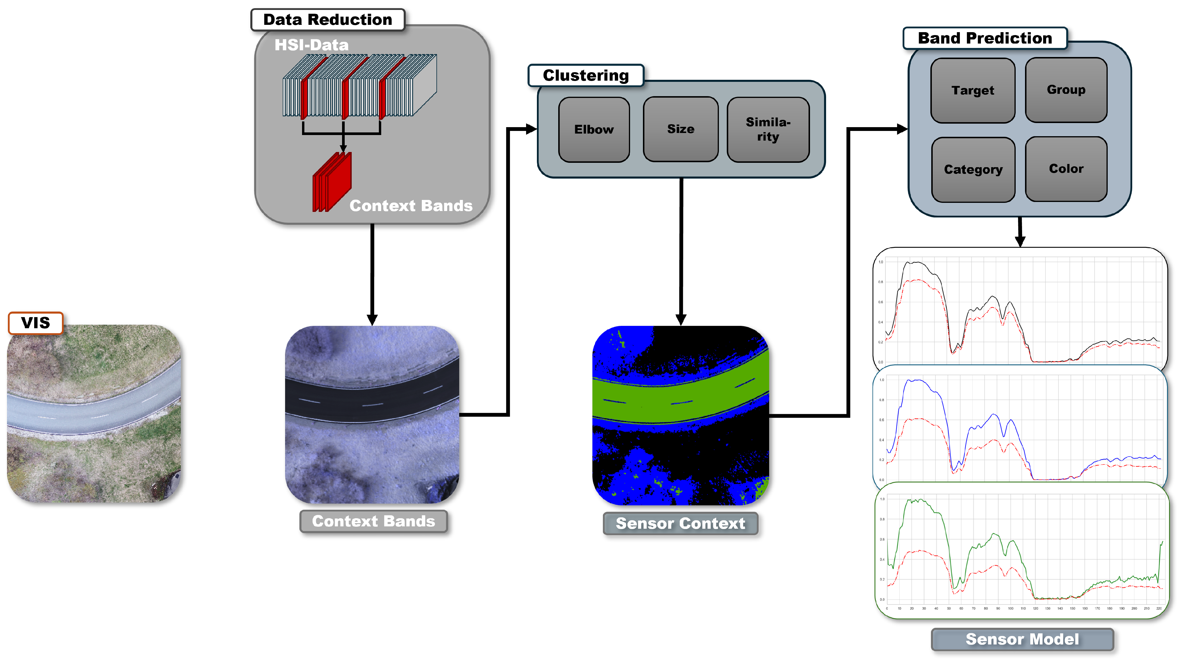
The methodology of sensor performance prediction consists of two main steps: (1) an iterative clustering that extracts the environmental sensor context and (2) the machine learning model that performs the actual performance prediction based on the inputs from (1). The approach uses the main environmental areas of an image and extracts for each of them the spectral vector and predicts with respect to them a deviation vector for the targets and their unknown location. These deviation vectors provide the information where the target anomaly is expected to be highest.

The complete process is illustrated in Figure 4, where the Sensor Context visualizes the extraction of the spectral signature of the environments in the image and the Sensor Model visualizes the prediction of the deviation vectors. In the example of Figure 4, the main environments are areas with meadow, trees, and a road. These areas are colored as black, blue, and green clusters and spectral signatures in the plots. The predicted deviation is shown as red vectors in the Sensor Model’s plots.

The detailed steps of the Sensor Performance Prediction works as following: In the first step, three bands are selected from the HSI dataset with N spectral bands, named context bands. These context bands are the input for the subsequent clustering process that extracts the sensor context. Choosing the three context bands as the clustering input reduces the spectral dimensionality and the K-means clustering runtime while maintaining the spectral differentiability to adequately distinguish the mean environmental regions. Afterwards, the actual clustering is performed by the K-means clustering algorithm, which provides a simple, efficient, and fast convergent method that can be applied to large datasets [47,48]. The K-means algorithm has four main processing steps: First, the initial number of clusters, k, must be defined. The algorithm then shuffles the input dataset containing w_n data points and randomly selects k data points as the initial centroids, referred to as c_k. In the third step, each data point w_i is assigned to its nearest cluster represented by the centroids. For this, the squared Euclidean distance between each data point, w_i, and each centroid, c_k, is calculated. The data points are then assigned to the centroids with the minimum distance. Then, the centroids are recomputed by taking the average of all assigned data points, w_ik, belonging to each cluster, k. The minimization of the squared distance and the recalculation of the centroids are repeated until no change in the assignment of the data points is observed or a maximum number of iterations is reached [49]. As mentioned previously, the K-means algorithm needs for the first processing step a specified number of clusters k. To define this initial cluster number, the elbow method for predicting it is used [50,51,52]. For this purpose, the K-means algorithm is processed with varying initial numbers of clusters. For each of them, the sum of the squared Euclidean distances, defined as Within-Cluster Sum of Squares (WCSS), is calculated with

$$\sum _{a=1}^k\sum _{i=1}^{m_a}\left|\right|w_{i,a}-c_a{\left|\right|}_2^2,$$

(1)

where m is the maximum number of data points w_i,k assigned to a cluster number k. The WCSS decreases as the number of initial clusters increases, and the optimal number of clusters can be determined by the elbow point, which marks a significant reduction in WCSS. As a result of the multiple K-means clustering performed to analyze the elbow point, each clustering process must be performed in a short processing time. Therefore, the HSI data are spectrally and spatially reduced by using the three context bands, which are spatially downsampled to a ground sampling distance (GSD) of 3.25 m only for the elbow analysis. In addition to the calculation of the elbow point, two other conditions are implemented for the assumption of the optimal cluster number. To extract the main areas of the sensor environment, the cluster size and spectral similarity of the centroids are checked to avoid undesired clusters. For instance, large objects and highly similar areas, such as trucks or age-related variations in road surfaces, should not form individual clusters. On the one hand, these objects occupy a relatively small area and are more integrated into the environment than separate entities, and on the other hand, the similarity is close enough to not result in changes in the band selection. Therefore, the cluster number determined by the elbow point is checked again, first for size and, if positive, also for similarity. The similarity is determined by the Euclidean distance and the Normalized Cross Correlation (NormXCorr) [53]:

$$\sum _{i=0}^a\left({\displaystyle \frac{(c_{i,l}-{\overline{c}}_l)\ast (c_{i,m}-{\overline{c}}_m)}{{\sigma }_{c_l}{\sigma }_{c_m}}}\right)·{\displaystyle \frac{1}{a-1}},$$

(2)

where, a represents the number of context bands, $\overline{c}$ denotes the mean of the centroid c, and σ_c represents the standard deviation of c. The variables l and m are the indices of the two centroids for which the NormXCorr is calculated. Note that after each failed check, the number of clusters is reduced by one, regardless of how many clusters failed, and the K-means algorithm is rerun with the reduced cluster number. If all checks are passed, the iteration is terminated and the result of the final K-means clustering is processed. Due to the initially reduced spectral depth, the determined centroids do not provide the spectral depth of N and have to be extended to the full spectral resolution of the HSI. For each centroid, the fifteen pixels with the highest similarity by Euclidean distance are determined and their full spectral signature in the initial HSI extracted and averaged. These averaged signatures then represent the environmental context in all N spectral bands. Now that the environmental context is defined, the centroids are processed using a machine learning model. Based on the target name, target group, target category, and visual target color, a random forest regressor predicts the expected target deviation of all extracted environmental areas, represented by the centroids, in the image for a set of known targets. The set of known targets used for model training is chosen to represent the expected targets in a real reconnaissance scenario and can be adapted for predicting unknown targets. The robustness of the model for predicting deviations for known and unknown targets in known and unknown environments has been tested and verified in [37] and achieved high accuracy results. Therefore, the method does not require mission- and target-specific training data and is ideally suited for the tactical air reconnaissance use case where target and mission area information is lacking. The dataset, targets, and training configurations of the model used here are the same as in the original paper and can be found there.

2.3. Band Selection

Once the target deviation of the bands has been predicted for each target, the important step of selecting the sensor bands for further processing follows. The band selection, together with the sensor context extraction and sensor performance prediction described in the previous section, forms the complete hyperspectral sensor management. In this step, the input bands are reduced to a spectral band set containing the most relevant target information for each target group in the actual sensor context. For this, the previous deviation vectors, which contain the expected target differentiability for all N spectral input bands, are analyzed and reduced to a vector of length five by considering only the five bands with the highest deviation within each vector. This provides a selection of the five best bands for each target known to the model and each environment extracted by the model. In the next step, this selection is divided into two subgroups, one containing predictions for targets of the target group UXO and the other containing predictions for targets of the target group camouflage materials. For these two subgroups, each reduced deviation vector within is further condensed to three bands per vector. The selection of these three bands is in such a way that the number of unique bands within the subgroup is minimal. Thus, as few bands as possible contain the target information for all targets and environments in the subgroup. In other words, from the five bands for each predicted deviation vector, the three bands that contain high information content for many targets in the different environments are selected. If for a target environment prediction and its three available selection slots no bands can be selected that are duplicated in any of the other vectors of the subgroup, the bands with the highest target deviation that have not yet been selected are automatically selected in descending order for these free slots. Thus, after completion of the selection procedure, a maximum of $3·n_t$ and a minimum of three bands can be selected for each subgroup with n_t targets. However, by considering three bands for each target–environment combination, it is ensured that even when reducing to the bands with high general information density but low target information for the target–environment combination under consideration, the selected bands still have a high target deviation for the specific combination, as at least the third best band of the combination is selected. At the same time, the amount of data is reduced as much as possible to allow fast processing for subsequent on-board processing. As a result of the band selection, two band sets, one for each target group, containing the unique bands from two reduction steps are created and later processed by the anomaly detectors.

2.4. Detectors

This section introduces the anomaly detectors and their methodology. The four detector groups used here are based on different approaches to achieve high performance results for a wide range of conditions and thus a high anomaly detection performance for a variety of mission and sensor contexts. The approaches of the detectors include the classical approach of anomaly detectors such as the Reed–Xiaoli (RXD) detector, but also clustering-based, correlation-based algorithms as well as signal filters from the field of signal engineering.

2.4.1. Reed–Xiaoli Detector

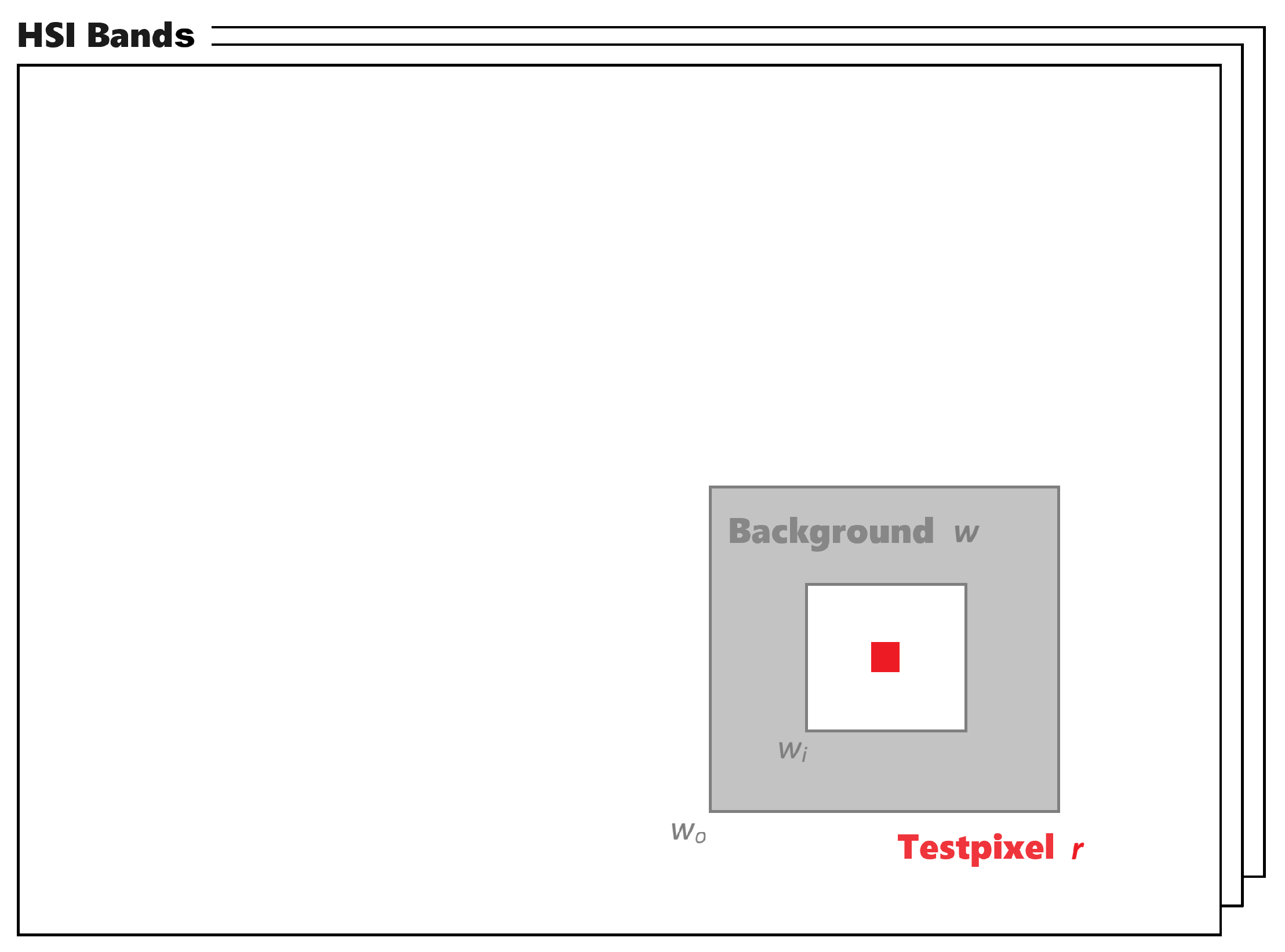
The RXD is one of the most popular and widely used anomaly detection algorithms. Due to its methodology, the RXD can be used unsupervised, without the need for training and detailed spectral target information [54,55,56]. These advantages make the detector very interesting for our presented use case, and therefore, it is selected as one of the implemented detectors. The RXD can be implemented as a global and a local variant. The global variant compares the anomaly of a single image pixel, called the test pixel r, with all other image pixels. The local RXD (LRX) used in this paper compares the test pixel with a predefined range of image pixels w through an inner and outer window, w_i and w_o, around it, see Figure 5.

Thus, the local RXD implementation identifies pixels that are significant with respect to their immediate surroundings and allows the extraction of small anomalies that are not significant compared to the whole image. The LRX works as follows [41]: For every pixel of interest r in the image, the squared Mahalanobis distance d_M² is calculated:

$$d_M{\left(r\right)}^2={(r-{\mu }_w)}^T{\sum }_w^{-1}(r-{\mu }_w),$$

(3)

where ${\mu }_w$ is the mean vector of the predefined local background area w and ${\sum }_w$ is the local covariance matrix. The local background area defined by the two windows is assumed in such a way that the size of the inner window is considered to be the size of the searched target in order to exclude it from the calculation of the background characteristics by ${\mu }_w$ and ${\sum }_w$. Thus, the Mahalanobis distance defines the distance of the spectral test pixel vector r from the mean spectral vector of the background ${\mu }_w$, taking into account the standard deviation of the background. Considering the standard deviation allows the Mahalanobis distance to evaluate the general deviation of the background and thus how anomalous and unique the test pixel is compared to this deviation and thus represents a true outlier. Once the Mahalanobis distance has been determined, a threshold can be set to determine whether a pixel is anomalous or normal. This can be performed by a fixed distance value or a percentage value t, depending on the general distances in the image. Finally, individual anomalous pixels are removed by morphological transformation. The process of erosion and dilation is defined by the kernel size ks, here with a size of (1,1).

2.4.2. Contour-Based HDBSCAN

A detection algorithm is a contour-based modification of HDBSCAN. It is called C-HDBSCAN. The underlying HDBSCAN is a hierarchical density based clustering algorithm [57,58]. Based on this, the HDBSCAN identifies clusters as areas of high and low density and separates them. In detail, clustering works as follows: In a first step, all distances d between a pair of data points are calculated. In our case, the Bray–Curtis distance was used for that. Subsequently, mutual reachability distances d_r are computed, which represent the local density of the data. For these, the minimum distance of the data points to a defined number of their neighbors is calculated, called the core distance d_c, which describes the density around it. Together with the Bray–Curtis distance, the mutual reachability distance can be calculated for points A and B by taking the maximum:

$$d_r(A,B)=max\{d_c\left(A\right), d_c\left(B\right), d(A,B)\}$$

(4)

By the end of this step, each data point is connected to all other data points through their mutual reachability distances, collectively forming mutual reachability distance graphs. In the next step, the graphs are used to create a minimum spanning tree (MST) by connecting all points to a graph with a total minimum d_r. This MST is processed through a hierarchical clustering, where each level of it represents a more detailed clustering. In the next step, the HDBSCAN analyzes these clusters for their density and thus how stable and significant they are. The clusters with the highest significance are selected as the final clusters, while the data points without cluster assignment or clusters with less than a predefined number of pixels, called c_min, are labeled as noise or anomalies. This can be used to create a binary cluster mask where the pixels assigned to noise are declared as ones and the rest as zeros. Due to its methodology, one of the main strengths of HDBSCAN is its ability to automatically determine the number of clusters. In addition, the algorithm is robust to varying data and densities and requires fewer parameters to be set. In addition, HDBSCAN is very good at identifying data points that do not belong to any cluster. This fact, combined with its robustness to varying data, makes HDBSCAN interesting for anomaly detection, and it is therefore used as one of the detectors in this paper. The HDBSCAN used here is implemented according to [59].

As mentioned above, the result of HDBSCAN is extended to the image contours, resulting in the contour-based HDBSCAN with an improved detection result. The contour information is extracted by Felzenszwalb and Huttenlocher image segmentation, which is a graph-based segmentation algorithm [60]. In the first step of segmentation, the image is transformed into a graph. The number of nodes in the graph is equal to the number of pixels in the image, while the connections, i.e., the edges between the nodes, represent the similarity of the pixels to each other. The similarity is determined by the color value of the pixels and their spatial distance. Based on this similarity, the segmentation algorithm identifies the segments of the image by starting to treat each pixel as a single segment and ending the segmentation process by assigning all segments below a defined similarity threshold as a single segment. The parameters scale_c and σ_c define the observation level and the Gaussian kernel preprocessing to control the level of detail for segmentation.

The Felzenszwalb segmentation algorithm is one of the most widely used algorithms and is characterized by its efficient segmentation. The implementation of the algorithm used in this paper is based on [61]. The result of the image segmentation is then transformed into a binary mask by thresholding the sizes of the segments, called a_max, with respect to the targets of interest. As a result, the two binary masks m_H and m_F generated by the HDBSCAN and the Felzenszwalb segmentation are combined in the final processing step by a logical AND operation ${\mathit{m}}_{\mathit{H}}\wedge {\mathit{m}}_{\mathit{F}}$ to produce the resulting binary detection map. For each contour with an associated anomalous cluster, the contour pixels are represented as ones in the final binary detection map.

2.4.3. Normalized Cross-Correlation Classification

Another detector is the Normalized Cross-Correlation Classification (NCC) based on [62]. As the name implies, NCC is a classifier that uses given spectral target signatures to classify their occurrence in the HSI. In the context of this paper, the NCC is redesigned as an anomaly detector due to the unknown target signatures and combined with additionally extracted image contours in the contour-based NCC (C-NCC). The method of the NCC can be explained as follows: The NCC receives as input the spectral signatures of the targets of interest as well as the spectral image. In the first step, both the spectral image and the target signatures are normalized to reduce the effects of external factors such as lightning. Then, each pixel is compared to the target signatures provided by calculating the NormXCorr. With this distance, the correlation to the targets of interest can be expressed for each pixel. Each pixel is assigned to the target with the highest NormXCorr, creating a classification map [62]. Pixels with a similarly low correlation can be declared as noise or anomalous by considering a threshold t. This is a percentage threshold that considers only a certain percentage of the pixels with the highest correlation. The general idea of NCC is therefore to assign the spectral image pixels to known spectral target signatures by determining the NormXCorr. This idea can be adapted as an anomaly detection algorithm. Based on the method of environmental context extraction introduced in Section 2.2.1, the sensor context and thus the environment is known. The targets of interest, camouflage materials and UXO, are different from this known environment. Therefore, the extracted spectral signatures of the environment from the process of BS are used as reference targets for the NCC. The camouflage materials and UXO must be pixels with a low correlation to the spectral signature of the environment and can be determined as an anomaly by applying the threshold described above, which determines a correlation that is too low to be part of the environment. Unlike the other detectors presented in this section, NCC includes the spectral signatures of the environment, i.e., the sensor context. Thus, NCC provides an additional way to detect anomalies in a broader context. Finally, the result of the NCC is transformed into a binary mask m_N by the predefined percentage threshold t and combined with the mask m_F of the extracted image contours as ${\mathit{m}}_{\mathit{N}}\wedge {\mathit{m}}_{\mathit{F}}$. The contours for the C-NCC are also extracted using the Felzenszwalb and Huttenlocher image segmentation and are provided by the same implementation used for the C-HDBSCAN.

2.4.4. Bandpass Filter

The final detector is the bandpass filter. Bandpass filters can be used for many applications but are often used in signal processing [63,64]. In the context of this paper, the bandpass filter is implemented as an anomaly detector. Image pixels that are significantly different from the background or the dominant environment are isolated by the bandpass filter through their spectral signature. Thus, spectral signatures outside a defined passable spectral range, defined by an upper and a lower cutoff, are attenuated or removed [65]. In the first step of the bandpass filter, the HSI with its multiple image bands is converted into a single 8-bit image band by taking the spectral average of each pixel. Then, the center of the image is determined based on the rows and columns of the pixels and the radius r of the image, calculated by

$$r=\sqrt{{{\displaystyle \frac{h}{2}}}^2+{{\displaystyle \frac{b}{2}}}^2},$$

(5)

where h is the number of image pixels in a column and b is the number of image pixels in a row. Based on the determined center and radius of the image, the initial percentage cutoff values l_l and l_h are transformed into a value range of the image space by multiplication with the image radius r. Then, based on the image rows and columns, the two 2-dimensional arrays x and y are created, which are the coordinate system for the subsequent Fourier transform:

$$x_i={\displaystyle \frac{-b}{2}}+i·{\displaystyle \frac{b}{b-1}},i=0,1,\dots ,b-1,$$

(6)

$$y_j={\displaystyle \frac{-h}{2}}+j·{\displaystyle \frac{h}{h-1}},j=0,1,\dots ,h-1,$$

(7)

$$x_{ij}=x_i,\forall j\in \{0,1,\dots ,\mathrm{h}-1\},$$

(8)

$$y_{ij}=y_j,\forall i\in \{0,1,\dots ,\mathrm{b}-1\}$$

(9)

Then the Euclidean distance d_r between the two arrays x and y is calculated. Based on the d_r and the previously calculated cutoff values of the image space, the actual bandpass filter f is created as a binary mask, where all distances within the cutoff ranges are set to zero and shifted to the center of the filter by

$$f_{\mathit{\text{shifted}}}(i,j)=f\left[\left(i+{\displaystyle \frac{h}{2}}\right)modh,\left(j+{\displaystyle \frac{b}{2}}\right)modb\right],$$

(10)

where f_shifted is the shifted filter. Now that the bandpass filter is determined, the actual Fourier transform of the image is performed by a 2-dimensional discrete Fourier transform. The product of the transformed image and the bandpass filter results in the filtered and transformed image, which is then transformed back into the original image space by an inverse 2-dimensional discrete Fourier transform. As a final step, the absolute values of the retransformed image are taken and converted into a binary mask by a percentage threshold t.

2.5. Processing Workflows

Now that the detectors have been introduced, the detailed processing steps for the different target groups, UXO and camouflage materials, can be described in detail. The general processing workflow of both target groups can be described as in Figure 6 and consists of two main parts, the preprocessing and the actual anomaly detectors. The basic preprocessing steps, such as spatial image reduction and Gaussian filtering, are performed to improve performance in terms of processing time and detection results.

2.5.1. Workflow for UXO

The anomaly detection workflow of the target group UXO, which is visualized in the upper part of Figure 6, consists of only two processing steps. In the first step, which is part of the preprocessing, the spatial resolution of the image is reduced to 70% of its inertial resolution. This results in a GSD of 0.093 m for the introduced dataset and is caused by the subsequent reduction in the processing time for the LRX detector that follows. The LRX detector, as a single detector within the group of anomaly detectors, performs the final anomaly detection results. Compared to the detection workflow for camouflage materials, the UXO detection workflow contains only one type of anomaly detector with different parameter settings. Due to the significantly different target characteristics caused by the size of the targets, only the LRX detector can provide a sufficient detection result and processing time. As will be shown later in the Section 3, the processing time for the target group UXO is significantly higher than that for the camouflaged materials. The range of suitable detectors was therefore narrowed down to the LRX, which demonstrated significantly the best detection performance with a short processing time in a preliminary study.

2.5.2. Workflow for Camouflage Materials

In contrast, the band set selection for detecting camouflage materials is depicted in an alternative workflow, which is shown in the lower part of Figure 6. The visual appearance of the materials varies greatly, necessitating more extensive preprocessing steps. In contrast to the target group UXO, the difficulty in detecting camouflage materials does not lie in the object size but in the variable spectral reflectance values within an object and often causes the typical visual camouflage print. Therefore, in addition to the downsampling step, which in this case is performed by reducing the internal images to 20% with a GSD of 0.325 m due to the larger target sizes, a Gaussian filter was implemented in the preprocessing. The Gaussian filter reduces the noise in the HSI and smooths the image [66,67]. In particular, larger natural anomalies such as reflections from tree canopies can be reduced. Even for images with poor lighting conditions that cause noise, often encountered in real reconnaissance missions like those in the dataset used here (Figure 3), the Gaussian filter can enhance the image quality, particularly with respect to the targets of interest and their characteristic contours. At the same time, the amount of computational resources is low. However, image objects of relatively large size are more likely to benefit from these advantages. Small objects, such as the second target group UXO, are often recognized as noise and filtered out. Thus, the Gaussian filter preprocessing is not applied to the UXO workflow.

The process of Gaussian filtering can be described in two main steps [65,68]. The first step is to define the Gaussian kernels. These kernels are a matrix representing a Gaussian distribution defined by the mean and the standard deviation. Next, the Gaussian kernels are applied to each image pixel, taking into account the neighboring pixels, by moving the kernel matrix along the image. The number of neighboring pixels is equal to the number of elements in the matrix, and each of them is assigned to one of the elements of the matrix. In a second step, a convolution of the considered image pixel is processed by multiplying the matrix with values of the image pixels and summing the products. The resulting sum is then divided by the sum of the matrix elements. The result of the convolution, the weighted average, replaces the original pixel value and results in the flattening and noise reduction effects of the filter. This process is repeated for all pixels, replacing all pixels with the weighted average. The implementation of the Gaussian filter used here is part of the Python package scipy.ndimage.gaussian_filter version 1.11.2 used with Python 3.10.14. The Gaussian distribution defined by the parameter $\sigma$ is set to 0.5. The resulting filtered image is the input for the following anomaly detectors, which were introduced in Section 2.4, and run with different parameter settings. However, it should be emphasized that only the LRX, C-HDBSCAN, and C-NCC use the preprocessing steps. The implemented bandpass filter processes the raw sensor bands. The reason for this is that firstly, due to the comparatively very fast processing, no reduction in spatial resolution is necessary, and secondly, an implementation of preprocessing would not lead to an increase in performance. The exact parameters of the algorithms presented here are presented in the following.

2.5.3. Detector Parameters and Settings

The detectors introduced in the workflow are used with varying parameter settings to assess their performance under different sensor contexts and to evaluate how changes in parameter settings influence the detectors’ performance.

Table 1. Parameters and settings of the detectors.

Detector	Parameter	Setting
UXO
	ID	1	2	3	4	5	6	7
LRX	t	0.9690	0.9790	0.9890	0.9990	0.9995	0.9997	0.9999
	wi	15	15	15	15	15	15	15
	wo	31	31	31	31	31	31	31
Camouflage Materials
	ID	1	2	3	4
LRX	t	0.9840	0.9890	0.9940	0.9990
	wi	51	51	51	51
	wo	101	101	101	101
	ID	5	6	7	8	9	10
C-HDBSCAN	cmin	15	15	15	15	15	15
	amax	70	70	70	70	70	70
	scalec	3,000,000	3,000,000	3,000,000	4,000,000	4,000,000	4,000,000
	σc	0.3	0.4	0.5	0.4	0.5	0.6
	ID	11	12	13	14	15	16	17	18
C-NCC	t	0.40	0.60	0.40	0.60	0.40	0.60	0.40	0.60
	amax	75	75	75	75	75	75	75	75
	scalec	3,000,000	3,000,000	3,000,000	3,000,000	4,000,000	4,000,000	4,000,000	4,000,000
	σc	0.3	0.3	0.4	0.4	0.5	0.5	0.6	0.6
	ID	19	20	21	22	23
Bandpass	t	0.995	0.995	0.995	0.995	0.995
	ll	0.02	0.02	0.02	0.02	0.04
	lh	0.06	0.07	0.08	0.09	0.09

shows the parameter settings sorted by the detector groups. Each detector and its setting is defined by a detector ID that is used as reference. The detector LRX is specified by the previously introduced percentage threshold parameters t and the inner and outer windows w_i and w_o. The window sizes are defined with respect to the sizes of the targets being searched. In a real reconnaissance scenario, the exact target size is usually unknown. Thus, a single window size that is suitable for many varying targets sizes is used and set as parameter. This is caused by the fact that varying the window sizes would require processing multiple LRX detectors for a single sample. Therefore, a single window size is selected for each target group that is suitable for all targets within the group. This size is defined as a constant parameter across all detector settings in each workflow, allowing the processing of a single LRX detector per sample. However, the threshold t varies for the different detector settings. This is due to the correlation of the sample characteristics, which leads to more or fewer false positives in the detection results, as well as the evaluation of the anomalous pixels, and therefore affects the optimal t. Unlike the LRX detector, the C-HDBSCAN parameter settings do not include a threshold. The C-HDBSCAN has a fixed minimum cluster size c_min and a fixed maximum contour size a_max. Both parameters depend on the size of the targets of interest and are optimized for variable sizes of expected targets in the reconnaissance mission and are therefore constant for the different settings. However, the parameters scale_c and σ_c vary for the different settings. These two parameters are also part of the varying parameters for C-NCC. Again, they control the important contour extraction. A constant a_max is used for all C-NCC settings. The value is slightly higher compared to the C-HDBSCAN. This is due to the characteristics of the C-NCC, which leads to higher detection performance with a slightly higher a_max. In addition, C-NCC is defined by a percentage threshold t. Pretests have shown that its variation leads to only small changes in the detection performance and is therefore almost constant for most settings, varying between 0.40 and 0.60. The last detector, the bandpass filter, is defined by a fixed percentage threshold t of 0.995. The detection performance is mainly controlled by the low and high cutoffs l_l and l_h. As a result of the Fourier transformation that filters the spectral signature in the defined cutoff range, the effect of image characteristics on the optimal threshold is reduced, and therefore so is the effect on detection performance.

3. Results

The Results Section is divided into three parts to analyze the correlation and performance of the BS, the anomaly detectors, and the mission and sensor context. First, the anomaly detectors and the different parameter settings are analyzed on their anomaly detection performance. On the one hand, the impact of the sensor context on the detection performance of the detectors and their combination is investigated. On the other hand, the general performance of the detectors is evaluated to demonstrate the suitability of their use for further testing. Subsequently, the performance of the Sensor Management and its BS is analyzed by considering context knowledge. For this purpose, the implemented BS is compared with a statistical band selection methodology and the use of the full set of bands by analyzing the detection results of the implemented detectors. The results provide insights into the impact of contextual knowledge on BS, determining whether no consideration, a general approach, or a dynamic selection provided by the Sensor Management can lead to improved anomaly detection performance. Finally, different combinations of architectures to connect the Sensor Management and the detectors are evaluated and recommendations for a managed system architectures of anomaly detectors are derived. All tests are CPU-based and run on Windows 11 with an Intel i7-1260P 12th Gen and 34 GB memory.

3.1. Performance Anomaly Detectors

As described in the Introduction, the performance of an anomaly detector changes with the targets themselves and their location, position, and image scene. Therefore, multiple anomaly detectors are used in this paper to improve the anomaly detection performance by selecting the best detector setting for each mission context. For this, the detection performance of each image and each of the detector settings in Table 1 is calculated by the weighted f₁-score, called f_$\beta$:

$$f_{\beta }={\displaystyle \frac{(1+{\beta }^2)\ast p\ast r}{{\beta }^2\ast p+r}},$$

(11)

where p is the precision and r the recall of the detection result. The weighting factor, $\beta$, is set to 1.1, which leads to a slightly higher prioritization of the recall and thus to a higher sensitivity. This is due to the planned architecture and the use case of camouflage and UXO detection. The detection process should be followed by a sensor context-based classification, which reduces false positives by taking the context into account. Therefore, a higher recall is preferred over a lower sensitivity, which results in a higher probability of undetected targets. In the context of the use case, an undetected UXO is also more destructive than a few more false positives. In addition to the f_$\beta$, the overall percentage of detected targets h_t in the samples is determined by dividing the total number of targets detected with at least one of each labeled target pixel by the number of labeled targets, whereas h_t determines the total detected target rate independent of the sample for the entire dataset, and $\overline{h}$_t determines the average target detection rate per sample. Furthermore, the calculated f_$\beta$ and the $\overline{h}$_t are added to a weighted sum, called f_h. For this purpose, weighting factors of 0.6 and 0.4 are used for h_t and f_$\beta$. The additional performance metric f_h is caused by the missing information of detected targets in the f_$\beta$. The f_$\beta$ score increases with the accuracy of the detected targets but does not distinguish the assignment of the detected target pixels. Thus, detecting one target in the sample with high accuracy can result in a f_$\beta$ score equal to detecting all targets in the sample with low accuracy. However, the latter is preferable in a tactical reconnaissance scenario, where the automated processing workflow assists by highlighting areas of interest, thereby reducing the sensor and missions operator’s workload and improving the total detection rate. Therefore, it is more important to detect as many targets in the scenario as possible than to detect a few targets and their contours with high accuracy, especially when the subsequent classification of the targets is based on spectral information rather than contours. This aspect is taken into account by the new metric f_h with the higher weight of h_t. These metrics are computed for each detector on dataset 1. For this purpose, each of them receives as input a selected set of bands depending on the assigned workflow and its target group. This band set recognizes the best minimum unique bands with respect to all extracted environments of one target group.

Table 2. Average detector performance per detector setting for dataset 1.

Detector	ID	$\overline{\mathit{p}}$	$\overline{\mathit{r}}$	$\overline{\mathit{f}}$$\mathit{\beta }$	$\overline{\mathit{h}}$t [%]	$\overline{\mathit{f}}$h
UXO
LRX	1	0.0015	0.6678	0.0033	80.95	0.4870
	2	0.0021	0.6435	0.0046	77.76	0.4684
	3	0.0038	0.6079	0.0083	74.97	0.4531
	4	0.0315	0.4366	0.0610	57.89	0.3717
	5	0.0518	0.3516	0.0898	51.09	0.3425
	6	0.0718	0.2906	0.1106	46.67	0.3242
	7	0.1143	0.1572	0.1166	32.93	0.2442
Best Setting	1	0.0015	0.6678	0.0033	80.95	0.4870
Camouflage Materials
LRX	1	0.0553	0.3514	0.0982	72.71	0.4755
	2	0.0723	0.3206	0.1189	67.73	0.4539
	3	0.1081	0.2685	0.1495	60.85	0.4249
	4	0.2085	0.1037	0.1202	40.51	0.2911
C-HDBScan	5	0.0142	0.3539	0.0266	54.59	0.3382
	6	0.0156	0.3629	0.0284	55.63	0.3451
	7	0.0135	0.3425	0.0259	56.11	0.3470
	8	0.0160	0.3338	0.0291	51.64	0.3215
	9	0.0145	0.3225	0.0285	50.68	0.3155
	10	0.0143	0.3054	0.0278	47.87	0.2983
C-NCC	11	0.0553	0.1744	0.0686	27.05	0.1898
	12	0.0642	0.1115	0.0688	16.28	0.1252
	13	0.0598	0.1666	0.0700	26.21	0.1852
	14	0.0700	0.1051	0.0693	16.09	0.1243
	15	0.0516	0.1396	0.0638	21.18	0.1526
	16	0.0591	0.0903	0.0605	12.44	0.0988
	17	0.0452	0.1164	0.0557	18.74	0.1347
	18	0.0467	0.0765	0.0496	11.35	0.0880
Bandpass	19	0.0760	0.1673	0.0993	42.56	0.2951
	20	0.0757	0.1686	0.0989	45.49	0.3125
	21	0.0751	0.1698	0.0982	47.35	0.3234
	22	0.0733	0.1690	0.0962	50.72	0.3428
	23	0.0505	0.1173	0.0639	46.33	0.3035
Best Setting	1	0.0553	0.3514	0.0982	72.71	0.4755

shows the average detector performance for the detector in Table 1 tested on dataset 1. For the target group of UXO, the highest score of $\overline{f}$_$\beta$ is achieved for the LRX detector with parameter setting ID = 7. However, for ID = 7 only an average of 32.93% targets per sample are detected for the dataset. This is the lowest value for all UXO detector settings. Therefore the highest $\overline{f}$_h is achieved for ID = 1 with 80.95% of average detected targets per sample, which is also the overall maximum. Furthermore, the results show relatively low precision values for all detector ID’s of the target group UXO, which means that many positive predictions are wrong, but this is also typical for the detection task of detecting small UXO in complex scenarios, see [43]. The detector settings for UXO contain relatively high thresholds t for the detection map, which means that many low significant anomalies are already left out. However, the targets are small, and the results show that even a few incorrectly predicted pixels relative to the few target pixels result in a low precision score. The recall score is in a higher value range. Again, the obtained scores show the expected performance values for the dataset and the recognition task. The evaluation of the detector settings by the determined $\overline{f}$_h would lead to a first rank of the detector with ID = 1, while the target pixels in the samples are correctly identified with a relatively high score of 0.6678 but so are many false-positive target predictions. This picture is similar for the camouflage detector settings.

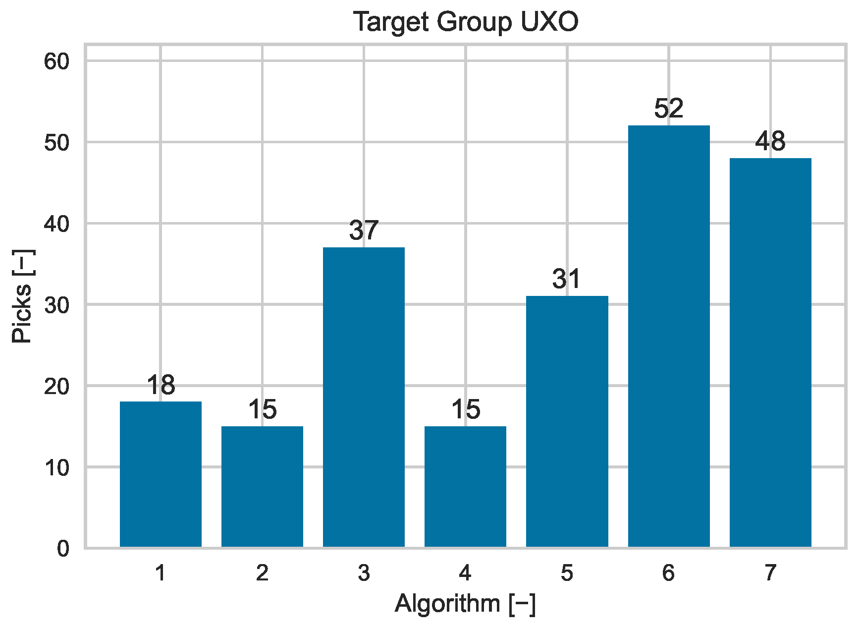
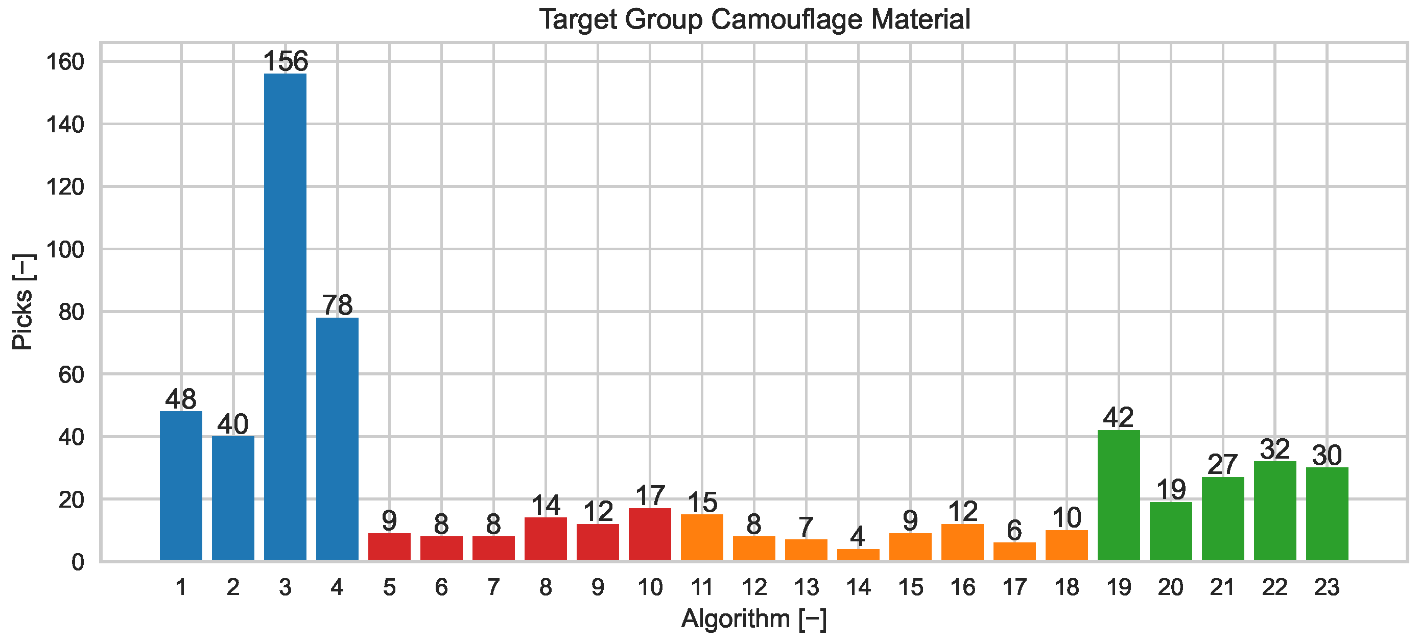
The precision scores of the detectors are also low. Since the target sizes are much larger and therefore large image areas must be falsely classified as positive, the low precision scores must be interpreted more critically. At the same time, the recall scores are higher and show a moderate performance. Overall, the $\overline{f}$_$\beta$- and $\overline{f}$_h-scores are comparable to the UXO results. However, a lower overall $\overline{h}$_t of 72.71 is achieved, suggesting that the performance is to be evaluated more critically. Regarding $\overline{f}$_h, the detector setting with ID = 1 has the highest total detection performance for dataset 1. The best performance results of the detector groups are determined for the LRX, followed by the C-HDBSCAN and the bandpass filter. Overall, there are small differences in performance, but none of the four detector groups can outperform the others, and the detector performances are generally low. Therefore, in addition to the general detector performances, the performance behavior of each detector is of particular interest. As already introduced, the detector performance changes with context, and thus, each detector has a sweet point with its highest detection performances. Therefore, the next step will be an analysis of how the consideration of this factor can lead to an improvement in the detection results. First, each image is analyzed by the $\overline{f}$_h-score for the detector with the best assigned detection performance. Figure 7 and Figure 8 visualize the instances where each detector achieved the highest performance across dataset 1. Only samples where at least one detector identified at least one of the targets were considered for this analysis. Otherwise, none of the detectors has a higher performance and can be evaluated as best.

For the UXO workflow, it can be seen in Figure 7 that the counts of selections are well distributed for all implemented detector settings. This means that all detector settings work best for specific contexts and can help improve overall detection results. The settings with ID = 6 and ID = 7 have the most selections and are slightly decreased. For the camouflage materials workflow, all detector settings are selected and can contribute to improve overall detection results. As visualized in Figure 8, the different detector settings are colored by detector group, where the counts of the LRX detector settings are colored in blue, the C-HDBSCAN in red, the C-NCC in orange, and the bandpass filter in green. Here, the distribution is more spread out, but there are more detector groups and settings available for a similar number of targets. The best-performing detector group is the LRX, followed by the bandpass filter. The C-HDBSCAN and the C-NCC have a lower number of selections, but for the few selections as best detector setting, they bring good performance results, see

Table 3. Average performance scores for the best selected detector settings on dataset 1.

Detector	ID	$\overline{\mathit{p}}$	$\overline{\mathit{r}}$	$\overline{\mathit{f}}$$\mathit{\beta }$	$\overline{\mathit{h}}$t [%]	$\overline{\mathit{f}}$h
UXO
LRX	1	0.0002	0.0718	0.0004	27.38	0.1644
	2	0.0009	0.3092	0.0019	64.81	0.3896
	3	0.0024	0.5794	0.0052	99.15	0.5970
	4	0.0250	0.4799	0.0499	100.00	0.6200
	5	0.0947	0.5245	0.1467	97.50	0.6437
	6	0.1889	0.6193	0.2818	97.00	0.6947
	7	0.2531	0.5421	0.3288	98.98	0.7254
Best Setting	total	0.0996	0.4407	0.1407	80.95	0.5420
Camouflage Materials
LRX	1	0.0075	0.0443	0.0136	27.27	0.1691
	2	0.0919	0.3065	0.1438	100.00	0.6575
	3	0.2495	0.5228	0.3316	100.00	0.7326
	4	0.6172	0.4572	0.4549	99.42	0.7785
C-HDBSCAN	5	0.0807	0.8167	0.1287	100.00	0.6515
	6	0.2193	0.7595	0.2681	100.00	0.7072
	7	0.0515	0.7166	0.0974	100.00	0.6390
	8	0.0952	0.8900	0.1635	93.75	0.6279
	9	0.0839	0.6361	0.1354	95.00	0.6242
	10	0.0654	0.6013	0.1153	96.88	0.6274
C-NCC	11	0.3972	0.6497	0.4476	98.33	0.7690
	12	0.4214	0.6862	0.4676	100.00	0.7871
	13	0.3391	0.5284	0.3710	85.71	0.6627
	14	0.4571	0.5671	0.3548	97.37	0.7261
	15	0.3443	0.6620	0.3940	95.24	0.7290
	16	0.5181	0.6970	0.5232	96.88	0.7905
	17	0.3099	0.7549	0.3914	94.74	0.7250
	18	0.4320	0.6800	0.4742	96.15	0.7666
Bandpass	19	0.1269	0.3171	0.1811	95.24	0.6439
	20	0.3799	0.6091	0.4751	97.22	0.7734
	21	0.2868	0.6113	0.3731	100.00	0.7492
	22	0.1976	0.8656	0.3397	100.00	0.7359
	23	0.1840	0.4392	0.1944	100.00	0.6778
Best Setting	total	0.2703	0.4912	0.2943	88.08	0.6462

. In addition to analyzing the distribution of detectors as the best performers, the overall detection improvement achieved by combining them is also examined. Here, for each sample, the best-performing detector, defined by the highest $\overline{f}$_h, is determined and selected for each sample of dataset 1. Thus, the detector varies dynamically with the actual context for each sample, leading to the results in Table 3. This table shows the average performance metrics for each detector in the cases where it was determined to be the best performer, as well as the overall average detection performance metrics independent of the detector. For that purpose, dataset 1 was used.

Regarding the camouflage material detectors, the following can be observed: The performance results within the C-NCC detector group are similar to the bandpass detector group. There are some slight differences, such as the generally higher precision score of C-NCC and the lower $\overline{h}$_t, but overall, none of the detectors within these two groups outperform the others. Looking at the counts of the best performers in Figure 8, it can be concluded that the C-NCC detectors have similar detection performance but are less robust to changes in mission context and have a smaller range of contexts with high detection performance compared to the bandpass detectors. However, the remaining two detector groups show slight differences. The C-HDBSCAN detectors have a relatively low precision and a slightly higher recall compared to the other groups. As a result, the $\overline{f}$_$\beta$ and $\overline{f}$_h scores are slightly lower, but again, the detector group and its detector are comparable to the others. Furthermore, C-HDBSCAN, like C-NCC, is a detector for very specific contexts, which can be seen in the distribution of Figure 8. The detectors of the LRX show a more spread-out performance, which is caused by the varying parameter t. The lower the significance of the target anomaly, the more false-positive classifications are taken into account, while at the same time the number of missing positively classified target pixels increases. This typical behavior can also be observed in the results for the LRX detectors of the UXO workflow. However, the $\overline{f}$_h is often below the others, while the LRX detector group has the highest number of best performers. Thus, the LRX detectors have a broad context where higher performance can be achieved and robust detection is possible.

Overall, the dynamic selections of detectors for each sample and its context show good performance scores for both target groups. The single detectors generally have a very high rate of detected targets per sample. This rate is much higher compared to the results in Table 2. Especially for the camouflage material, there are great improvements in the detection accuracy. All scores, the precision, the recall, $\overline{f}$_$\beta$ and $\overline{f}$_h, are higher than before. This causes a high $\overline{f}$_$\beta$ and $\overline{f}$_h, which show great results and robust detection performance for the challenging mission contexts of the camouflage materials in dataset 1. The overall detection result for dynamic contextual selection is significantly improved for all metrics. Due to the targeted selection, the rate of detected targets per sample is improved to 88.08%, while precision, recall, and $\overline{f}$_$\beta$ are also improved compared to the best single detector with the ID = 1 in Table 2. The dynamic selection of the detector thus leads to large improvements in detection performance.

The target group UXO shows good improvements in the detection results too. For the individual detectors, the UXO target group does not exhibit as significant an increase in precision and recall scores as the camouflage materials. However, overall, the $\overline{f}$_h score has improved. With context knowledge and the dynamic selection, an overall result of 0.1407 for $\overline{f}$_$\beta$ and 0.5420 for $\overline{f}$_h was achieved with no loss of detected targets, which is a significant improvement over the results of the best single detector ID = 1 in Table 2. Although the recall has been reduced, the loss has been compensated by a higher recall, resulting in the higher $\overline{f}$_$\beta$. Overall, the dynamic selection of detectors for detecting UXO can increase the challenging detection precision under preservation of the detected targets. Due to the high h_t-scores, many targets in the dataset were detected, which is even more important here. Without target detection, no detection can be achieved, even with postprocessing optimization. Thus, the result of still-low precision scores must be considered and emphasized for further system architecture, postprocessing steps, and high accuracy in the final target classification. This importance is much higher compared to camouflage materials, where these efforts can be reduced in this development of system design. Concluding the results, the evaluation shows a great impact of the context on the detector performance. A context-based and targeted selection of the detectors by the introduced metric f_$\beta$ can improve the detection results significantly and should be part of future system architectures.

3.2. Performance Sensor Management

Next, the performance improvements achieved by considering context knowledge for BS are investigated. For this analysis, the introduced Sensor Management is evaluated and analyzed based on the previous detectors and their context selection. The selected sensor bands identified by the Sensor Management are compared with the anomaly detection performance of the full band set and a statistically determined band set.

First, the anomaly detection performance of the BS in the Sensor Management is analyzed and compared to the processing of all 224 HSI sensor bands simulating a missing BS. Due to the hundreds of bands that must be processed in this test, it consumes a large amount of processing resources and processing time, denoted as t_p. Therefore, the test is performed only for the previously identified best detector of each target group. For UXO and camouflage material, it is the detector with ID = 1 both times. The tests were carried out on dataset 1, and the results are visualized in

Table 4. Comparison of RX anomaly detector performance with all spectral bands (HSI bands) and by the BS model-selected bands (BS bands).

Target Group	Score	HSI Bands	BS Bands	Relative [%]
UXO	$\overline{p}$	0.0001	0.0015	50.00
	$\overline{r}$	0.0425	0.6678	1471.29
	$\overline{f}$$\beta$	0.0002	0.0033	1550.00
	ht [%]	8.76	80.51	819.06
	$\overline{f}$h	0.0458	0.4870	963.32
	$\overline{t}$p [s]	242.90	1.45	−99.40
Camouflage material	$\overline{p}$	0.0048	0.0553	1052.08
	$\overline{r}$	0.0401	0.3514	776.31
	$\overline{f}$$\beta$	0.0087	0.0982	1028.74
	ht [%]	22.49	72.88	224.06
	$\overline{f}$h	0.1324	0.4755	259.14
	$\overline{t}$p [s]	19.88	0.11	−99.45

. When analyzing these performance metrics, the significantly higher detection performance of Sensor Management stands out. The determined relative performance differences show high deviations for all metrics in favor of the BS. Especially for the challenging target group UXO, the relative deviations are the highest. Processing all sensor bands will result in lower average precision, recall, $\overline{f}$_$\beta$, and, most importantly, significantly fewer detected targets and therefore lower $\overline{f}$_h. Considering the higher processing requirements, the use of all sensor bands via Sensor Management is not recommended.

The next test therefore examines whether the Sensor Management, and its context-based BS also offers an advantage over statistical BS. For this purpose, the statistically best bands are determined for dataset 1 and dataset 2, and thus for both of the previously introduced testsites. Therefore, for each target in each sample of the dataset, the target deviation is calculated by taking the absolute value of the subtraction of the target’s immediate environment and the average target vector. The target’s immediate environment is represented by the associated environment cluster centroid c_k, which is also the reference vector for the target deviation. This determined deviation is then reduced for each target and each sample to the three best bands with the highest target deviation. Then, from these sets of best bands, the unique bands for the targets within the two target groups are determined. This analysis is performed for both datasets and results in the following

Table 5. Determined statistically best band for testsites 1 and 2 and the two target groups.

Target Group	Testsite	Targets	Bands
UXO	1	9 to 15	27–30
	2	9 to 15	17–19, 28–32
Camouflage Material	1	1 to 8	15–18, 27–31
	2	1 to 8	17–19, 23, 27, 28, 20, 83

.

Based on these statistically best bands and the dynamic, context-based bands selected by the Sensor Management, the anomaly detection performance is evaluated for two reconnaissance scenarios. In the first scenario, the targets and the mission environment are known from previous reconnaissance flights. Therefore, the Sensor Management is trained for the mission environment and the targets with a dataset containing the targets and the mission environment. The statistically best bands are also determined for this dataset and are also known for the reconnaissance mission. This scenario is simulated with dataset 1 for testsite 1. For each of the dataset samples, the Sensor Management predicts a band set to be processed by the best-performing detection algorithm for that sample. The same procedure is performed for the statistically best bands of the two target groups for the first testsite. The evaluated performance metrics are visualized in

Table 6. Comparison of detection performance with statistically selected bands and dynamically selected bands by the Sensor Management for testsite 1 and dataset 1.

Target Group	Score	Stat. Bands	BS Bands	Relative [%]
UXO	$\overline{p}$	0.068	0.100	47.06
	$\overline{r}$	0.400	0.441	10.25
	$\overline{f}$$\beta$	0.098	0.141	43.88
	ht [%]	75.71	80.51	6.34
	$\overline{f}$h	0.495	0.542	9.49
Camouflage material	$\overline{p}$	0.327	0.270	−17.43
	$\overline{r}$	0.478	0.491	2.72
	$\overline{f}$$\beta$	0.331	0.294	−11.18
	ht [%]	88.32	88.06	−0.29
	$\overline{f}$h	0.664	0.646	−2.71

, where the column “Stat. Bands” represents the detection results of the statistically selected bands and the “BS Bands” column represents the results of the dynamically selected bands by the Sensor Management.

The results show significantly better anomaly detection results for the Sensor Management and the target group UXO. As visualized by the relative improvements in the last column, the performance increase in detected targets h_t must be emphasized. Because of the Sensor Management, many more targets can be found, which is a critical metric in reconnaissance missions. Furthermore, the other performance metrics can also be improved, and the Sensor Management can outperform the statistical approach. However, this performance improvement is not achievable for the camouflage material. Here, the statistical approach leads to higher detection performance. The precision of the detections with the statistical bands is higher, while the recall is lower. This can be a result of the Sensor Management’s methodology, where the model is trained only to predict the bands with a respective high deviation from the environment. The characteristics of the background, such as uniformity, are not taken into account. Therefore, it is possible that the Sensor Management’s bands have a lower uniformity and therefore more background anomalies, which can lead to a lower precision score but a higher recall due to the higher target information. The high precision score of the statistical approach leads to a higher $\overline{f}$_$\beta$ and also to a higher $\overline{f}$_h. The number of targets detected differs for only one target. Due to the small difference, it is difficult to interpret this as a performance improvement due to the statistical approach alone. Such small deviations can be caused by many influences such as hardware, rounding errors, etc., and are difficult to reproduce by recalculation. The results rather indicate that the statistical bands are more beneficial for background uniformity and the Sensor Management is more beneficial for target contour accuracy, but the target information is nearly equal for both approaches and not high enough for fundamental differences in the number of detected targets. In contrast to the small UXO, a few falsely negative classified pixels of the large camouflage materials do not lead to a complete lack of target detection in the form of a significantly changed h_t as quickly. Overall, the statistical approach has slightly better detection performance but does not outperform Sensor Management.

The next scenario simulates a reconnaissance mission in an unknown area with partially unknown targets. Often, many of the targets of interest have been seen before in another reconnaissance mission and are already known in some way but not in the actual specific mission context. Thus, in the second scenario, some targets are known, while the mission area is completely unknown. For this purpose, the Sensor Management is trained on the first dataset and the statistical bands are evaluated for the first dataset. Then, both approaches are tested on dataset 2 with its unknown testsite and the additional and unknown targets that were not part of dataset 1. The results of this analysis can be found in

Table 7. Comparison of the average detection performance with statistically selected bands and dynamically selected bands by the Sensor Management configured on dataset 1 and tested on dataset 2.

Target Group	Score	Stat. Bands	BS Bands	Relative [%]
UXO	$\overline{p}$	0.008	0.021	162.50
	$\overline{r}$	0.232	0.329	41.81
	$\overline{f}$$\beta$	0.015	0.035	133.33
	ht [%]	77.00	89.00	15.58
	$\overline{f}$h	0.469	0.545	16.20
Camouflage material	$\overline{p}$	0.271	0.283	4.43
	$\overline{r}$	0.413	0.438	6.05
	$\overline{f}$$\beta$	0.261	0.287	9.96
	ht [%]	95.82	95.82	0.00
	$\overline{f}$h	0.688	0.699	1.60

. Again, the Sensor Management outperforms the statistical approach for the UXO. The performance values of all metrics are significantly higher for the Sensor Management, and the relative performance improvements are increased compared to the first reconnaissance scenario. In this more challenging scenario, the statistical approach is less applicable and the rate of detected targets is relatively improved by 77.00% to a high absolute value of 89.00%. The Sensor Management’s model can transfer the knowledge much better to the scenario and is able to select the sensor bands that lead to a significantly higher anomaly detection performance. Furthermore, the Sensor Management has higher detection performance for the camouflage materials as well. In this case, the statistically selected bands perform worse for all performance metrics except for h_t. Again, the same performance was found for both approaches. Overall, the relative performance differences for this target group have increased compared to the first scenario. The performance improvements are not significant and only slight, but the same tendency of higher robustness and adaptability of the Sensor Management for use cases with lower correlation with previous training or configuration scenarios can be observed. However, none of the approaches can outperform the other for camouflage materials, but the performance improvements of Sensor Management are significant enough to recommend its use. Again, the results can be interpreted as the target sizes allow for an equal detection hit rate, and the different approaches can only change the performance metrics in terms of precision and recall.

For the evaluation of the sensor management performance, it can be concluded that the methodology of context-based band selection brings significant detection performance improvements with respect to the full band set. With respect to a statistical approach, the significant improvements can also be observed for the target group of UXO. The more the actual scenario differs from the initial training and configuration scenario, the more the benefits of Sensor Management become apparent. However, a performance improvement through Sensor Management can only be achieved for unknown mission scenarios with the camouflage materials. The model shows slightly higher performance values for this use case and seems to be more robust. The amount of training the model and analyzing the statistical best bands is the same for the methods used here in this paper. Due to the higher robustness for unknown mission scenarios and therefore a higher variability for changing mission scenarios, the Sensor Management can be recommended for all use cases.

3.3. Performance of Architectural Design

Now that the performance of the Sensor Management has been evaluated, the interaction between the Sensor Management and the detector architecture is examined. In the previous test, the model predicted a set of bands for each target group based on all known targets and all environments in the sample, and the anomaly detector was analyzed for the entire image scene. Due to the Sensor Management’s methodology, the different environments within a sample can be distinguished and predicted by the model. Therefore, it should be investigated if a more detailed decomposition of the BS into several band sets, one for each environment, can improve the anomaly detection performance. Thus, two different architectures are implemented. The first architecture corresponds to the previous tests, with one band set per audience for all environments in the scene. The second architecture provides as many band sets per target group as there are environments in the image scene. The methodology of band selection is similar, but this time the selection is made separately for each environment area, resulting in multiple band sets. In addition, this test is designed to examine the impact of architecture. Therefore, the sensor model’s prediction is considered only for the targets that are actually in the sample, so the performance results are not affected by the prediction for targets that are not in the sample, and only the effect of the environment breakdown can be observed. Multiple band sets are also used to process multiple anomaly detectors. For each extracted environment, the best-performing anomaly detector is processed with the assigned band set, resulting in multiple detection maps for a single sample. Those areas of the resulting detection maps that are not assigned to the corresponding environment are masked. Subsequently, the performance metrics of the masked detection maps are determined with respect to the likewise masked label mask and for each environment and each sample. This second architecture allows the use of a specific anomaly detector in addition to the specific band sets for each environment. In this way, the effect of a more detailed architecture based on the sensor context can be investigated. In addition to the two architectures focusing on this influence, the influence of a further separation of the camouflage materials into improvised and military materials is also tested and combined for both architectures. The workflow and detectors introduced in Section 2.5 are the same, but the band selection process and the processing by the anomaly detectors are split into a different target group. The results of the test on dataset 1 are presented in

Table 8. Detection performance results for varying processing architectures.

Target Group	Score	All Env.	Per Env.	Relative [%]
UXO	$\overline{p}$	0.101	0.077	−23.76
	$\overline{r}$	0.454	0.220	−51.54
	$\overline{f}$$\beta$	0.142	0.100	−29.58
	ht [%]	84.46	48.31	−42.80
	$\overline{f}$h	0.563	0.342	−39.25
	$\overline{t}$p [s]	1.20	0.58	−51.67
Camouflage material	$\overline{p}$	0.236	0.087	−63.14
	$\overline{r}$	0.451	0.191	−57.65
	$\overline{f}$$\beta$	0.257	0.111	−56.81
	ht [%]	87.03	52.66	−39.49
	$\overline{f}$h	0.624	0.365	−41.51
	$\overline{t}$p [s]	0.12	0.04	−66.67
Improvised camouflage	$\overline{p}$	0.242	0.100	−58.68
	$\overline{r}$	0.583	0.294	−49.57
	$\overline{f}$$\beta$	0.302	0.147	−51.32
	ht [%]	96.09	64.96	−32.40
	$\overline{f}$h	0.697	0.428	−38.59
	$\overline{t}$p [s]	0.11	0.05	−54.55
Military camouflage	$\overline{p}$	0.231	0.056	−75.76
	$\overline{r}$	0.350	0.076	−78.29
	$\overline{f}$$\beta$	0.216	0.062	−71.30
	ht [%]	80.51	48.62	−39.61
	$\overline{f}$h	0.569	0.317	−44.29
	$\overline{t}$p [s]	0.13	0.04	−69.23

, where the first column shows the prediction results for targets in the samples without the additional split, and the second column shows the results with the additional split in their environments.

The results show that an architecture based on a more detailed subdivision based on environment areas does not lead to performance improvements. The number of detected targets is significantly lower, as are the precision and recall values. Only the processing time is lower due to the smaller band sets. In general, the more detailed architecture allows multiple anomaly detection tasks and thus a better possibility of computational parallelization. However, the performance values are too low to recommend this architecture. This is not the case for the additional separation of improvised and military camouflage materials into two target groups. There are good performance improvements for the first architecture. Besides the processing time, all metrics are increased and more targets can be detected with higher precision and recall. With the further separation into two groups of camouflage materials, the rate of detected targets can be improved from 87.03% to a total rate of 88.20% for all camouflaged targets. Even with an almost constant processing time, the less detailed target groups with their fewer detection tasks do not necessarily lead to an advantage in terms of computational costs. Again, the additional target group and its additional detection task allows for a possible computational parallelization and does not have to cause negative effects. Overall, an architecture that considers the available environments per image and performs a BS and detector selection based on this is the most advantageous. An additional subdivision into further target groups with their own processing workflows can also have a positive effect. On the other hand, too much detail of the sensor contexts in the form of detailed dependent process chains overweights the sensor context and is not recommended.

4. Discussion

Analysis of the results has shown that the implemented detection workflows with the multiple detectors and their settings produce good detection results through dynamic context-based selection based on the highest f_h, see Table 3. The dynamic detector selection based on this metric results in a large detection improvement compared to the static detectors in Table 2. However, the calculation rule of f_h results in determined values for the detectors that are sometimes difficult to interpret. For example, the determined $\overline{f}$_h for the algorithm with ID = 7 for the target group UXO in Table 3 has a value of 0.7254 at 98.98% $\overline{h}$_t and an $\overline{f}$_$\beta$ of 0.3288. At the same time, the camouflage detector with ID = 17 has a very similar $\overline{f}$_h of 0.7250, but the corresponding $\overline{h}$_t is 94.74% with an $\overline{f}$_$\beta$ of 0.3914. Thus, the results show that the metric is suitable for selecting the best detector setting, but it is not an appropriate metric for interpreting the actual anomaly detection performance. Furthermore, the metric of f_h leads to a strong focus on the rate of detected targets at the expense of losses for the f_$\beta$ score. Other aspects of possible preferred detection characteristics, such as the number of misclassified areas instead of the raw pixel count, are not taken into account. For an operational system use, it might be more beneficial to have a few regions of interest that need to be checked by a human operator than to have a few pixels in more regions of interest. From this point of view, the metric f_h could be part of further research. Besides the way of selecting the detector, the final detection performance itself could be discussed. As already highlighted, the rate of detected targets and the achieved recall scores for both target groups are good, especially with respect to the dataset with the characteristics of real data and the challenging detection task by itself. However, the precision score of the UXO target group is improved by the detector variations but is still very low. On the one hand, this is typical for the type of detectors used in this paper, and on the other hand, the target sizes must be highlighted. Due to the spatial resolution of the sensor, the target information of the group UXO is often provided by only 10 to 15 pixels. Therefore, low precision results are quickly determined by only a few false classifications. This makes targeted postprocessing all the more important. At this stage, only the areas or pixels of interest are identified. There is still no classification of the type of target, which is crucial for reconnaissance tasks. In addition, important information and very specific knowledge, such as the spectral signature, the biggest advantage of HSI, has not yet been considered and implemented in the workflow. With this unused information, it is very likely that false-positive classifications will be significantly reduced. The contours of the targets themselves are already detected with good accuracy, and this is even more crucial with respect to the possibility of postprocessing and unused information. Undetected targets at this stage of processing will remain undetected. Therefore, the detection results can be considered very good from this point of view. Besides the partly low precision score, another aspect was mentioned in the previous section. The method of band selection uses the predicted bands with the highest deviation from the target. Other characteristics of the bands, such as the previously mentioned uniformity of the bands, are not taken into account. The results in this paper can be interpreted as indications for further research. However, they can hardly be considered as more than indications. Therefore, further research should investigate whether additional band characteristics can positively influence the anomaly detection performance. Another aspect that should be discussed is the performance evaluation of the last test in Section 3.3. The performance results of the architecture with more detailed attention to the extracted environment have a significantly lower performance. This performance is determined with the metrics by masking environment areas that are not of interest. Based on these metrics, the best detectors for each image and its regions are selected and included in the overall evaluation. This may not be the best approach and could lead to the strong performance deviation of the tested architectures. The implemented masking leads to a selection of detectors that show good results only for the actual area of interest. For the other areas, especially those without a target, the performance of the selected detector is not taken into account and a detector with a low detection rate is simply selected. This detector can be a detector that has a low detection rate because in principle no detection takes place. For example, the LRX could be implemented with a very low t. This detector would not be able to detect the targets for many samples, but the detector will most likely be chosen as the best detector for image regions without targets due to the low threshold and the resulting low pixel classifications. Therefore, it might be advantageous to adjust the performance estimation. However, the performance estimation is adequate. The idea of the more detailed architecture is to select the detectors that are only suitable for the surrounding areas. Therefore, it is legitimate to neglect the detector classification of the other areas. For the areas without a target, it is not possible to prevent the described behavior, but that is not of interest. The test was performed to investigate the performance improvement of the more detailed architecture. However, since there is no improvement despite this logic gap, which is very advantageous for performance, it can be assumed that this will not be the case even if the metric is changed given the large differences in performance, and the architecture with a higher level of detail is still not recommended for application. Therefore, the final score remains unchanged.

5. Conclusions

In this paper, the Sensor Management with a dynamic BS as well as different anomaly detectors and their workflows for the detection of UXO and camouflage materials is introduced. The Sensor Management and the detector workflows were evaluated with respect to their performance. The results showed that the dynamic BS of the Sensor Management outperformed the anomaly detection performance using all available HSI sensor bands. For the target group of UXO, the Sensor Management was able to generate significant anomaly detection performance improvements and also outperformed a statistical band selection in all tested scenarios. This performance advantage was less for the camouflage materials. Here, the statistical approach gives slight advantages for reconnaissance scenarios with previously known targets and mission environment. However, more complex scenarios with partially unknown targets and an unknown mission environment can be better handled by the Sensor Management. Overall, the use of an implemented Sensor Management results in clear advantages in anomaly detection performance and should be part of an operational system architecture for the reconnaissance tasks investigated here. The same applies to the anomaly detectors and their workflows. The results showed an improvement in anomaly detection performance by the approach of implementing multiple detector settings with a targeted selection for each image. This dynamic detector selection has good performance results for both target groups and allows a high detection rate of targets, even for the small UXO. However, the architectural design of an operating system for UXO detection should focus on an effective postprocessing to identify falsely positive classified areas by their actual unused spectral information. In addition, a further separation of the target group of camouflage materials into military and improvised camouflage materials as well as the target group of UXO is recommended for a system architecture. A higher level of detail with respect to the extracted sensor context and its environment is not advantageous and must not be considered. Nevertheless, it can be concluded that the integration of contextual knowledge can bring significant performance benefits to both the BS and the anomaly detectors and could be recommended.

References

1. Lu, B.; Dao, P.; Liu, J.; He, Y.; Shang, J. Recent Advances of Hyperspectral Imaging Technology and Applications in Agriculture. Remote Sens. 2020, 12, 2659. [Google Scholar] [CrossRef]
2. Zhu, W.; Sun, Z.; Yang, T.; Li, J.; Peng, J.; Zhu, K.; Li, S.; Gong, H.; Lyu, Y.; Li, B.; et al. Estimating Leaf Chlorophyll Content of Crops via Optimal Unmanned Aerial Vehicle Hyperspectral Data at Multi-Scales. Comput. Electron. Agric. 2020, 178, 105786. [Google Scholar] [CrossRef]
3. Liu, L.; Dong, Y.; Huang, W.; Du, X.; Ma, H. Monitoring Wheat Fusarium Head Blight Using Unmanned Aerial Vehicle Hyperspectral Imagery. Remote Sens. 2020, 12, 3811. [Google Scholar] [CrossRef]
4. Cai, J.; Meng, L.; Liu, H.; Chen, J.; Xing, Q. Estimating Chemical Oxygen Demand in Estuarine Urban Rivers Using Unmanned Aerial Vehicle Hyperspectral Images. Ecol. Indic. 2022, 139, 108936. [Google Scholar] [CrossRef]
5. Marques, M.M. STANAG 4586—Standard Interfaces of UAV Control System (UCS) for NATO UAV Interoperability; North Atlantic Treaty Organization: Brussels, Belgium, 2012. [Google Scholar]
6. Hupel, T.; Stütz, P. Adopting Hyperspectral Anomaly Detection for Near Real-Time Camouflage Detection in Multispectral Imagery. Remote Sens. 2022, 14, 3755. [Google Scholar] [CrossRef]
7. Thenkabail, P.S.; Lyon, J.G. Hyperspectral Remote Sensing of Vegetation; CRC Press: Boca Raton, FL, USA, 2012. [Google Scholar]
8. Nasrabadi, N.M. Hyperspectral Target Detection: An Overview of Current and Future Challenges. IEEE Signal Process. Mag. 2014, 31, 34–44. [Google Scholar] [CrossRef]
9. Manolakis, D.; Shaw, G. Detection Algorithms for Hyperspectral Imaging Applications. IEEE Signal Process. Mag. 2002, 19, 29–43. [Google Scholar] [CrossRef]
10. Camps-Valls, G.; Tuia, D.; Bruzzone, L.; Benediktsson, J.A. Advances in Hyperspectral Image Classification: Earth Monitoring with Statistical Learning Methods. IEEE Signal Process. Mag. 2014, 31, 45–54. [Google Scholar] [CrossRef]
11. Pastor, E.; Lopez, J.; Royo, P. UAV Payload and Mission Control Hardware/Software Architecture. IEEE Aerosp. Electron. Syst. Mag. 2007, 22, 3–8. [Google Scholar] [CrossRef]
12. Bajcsy, P.; Groves, P. Methodology for Hyperspectral Band Selection. Photogramm. Eng. Remote Sens. 2004, 70, 793–802. [Google Scholar] [CrossRef]
13. Adão, T.; Hruška, J.; Pádua, L.; Bessa, J.; Peres, E.; Morais, R.; Sousa, J. Hyperspectral Imaging: A Review on UAV-Based Sensors, Data Processing and Applications for Agriculture and Forestry. Remote Sens. 2017, 9, 1110. [Google Scholar] [CrossRef]
14. Wang, Q.; Zhang, F.; Li, X. Optimal Clustering Framework for Hyperspectral Band Selection. IEEE Trans. Geosci. Remote Sens. 2018, 1–13. [Google Scholar] [CrossRef]
15. Sun, W.; Du, Q. Hyperspectral Band Selection: A Review. IEEE Geosci. Remote Sens. Mag. 2019, 7, 118–139. [Google Scholar] [CrossRef]
16. Sneha; Kaul, A. Hyperspectral Imaging and Target Detection Algorithms: A Review. Multimed. Tools Appl. 2022, 81, 44141–44206. [Google Scholar] [CrossRef]
17. Chang, C.I. Hyperspectral Data Processing: Algorithm Design and Analysis; John Wiley & Sons: Hoboken, NJ, USA, 2013. [Google Scholar]
18. Bioucas-Dias, J.M.; Plaza, A.; Camps-Valls, G.; Scheunders, P.; Nasrabadi, N.; Chanussot, J. Hyperspectral Remote Sensing Data Analysis and Future Challenges. IEEE Geosci. Remote Sens. Mag. 2013, 1, 6–36. [Google Scholar] [CrossRef]
19. Chang, C.I. Target-to-Anomaly Conversion for Hyperspectral Anomaly Detection. IEEE Trans. Geosci. Remote Sens. 2022, 60, 1–28. [Google Scholar] [CrossRef]
20. Chen, J. (Ed.) Processing and Analysis of Hyperspectral Data; IntechOpen: London, UK, 2020. [Google Scholar] [CrossRef]
21. Chetia, G.S.; Devi, B.P. Endmember Extraction with Unknown Number of Sources for Hyperspectral Unmixing. In Computer Vision and Image Processing; Gupta, D., Bhurchandi, K., Murala, S., Raman, B., Kumar, S., Eds.; Communications in Computer and Information Science; Springer International: Berlin/Heidelberg, Germany, 2023; Volume 1776, pp. 567–578. [Google Scholar] [CrossRef]
22. Plaza, A.; Chang, C.I. Impact of Initialization on Design of Endmember Extraction Algorithms. IEEE Trans. Geosci. Remote Sens. 2006, 44, 3397–3407. [Google Scholar] [CrossRef]
23. Plaza, A.; Valencia, D.; Plaza, J.; Chang, C.I. Parallel Implementation of Endmember Extraction Algorithms From Hyperspectral Data. IEEE Geosci. Remote Sens. Lett. 2006, 3, 334–338. [Google Scholar] [CrossRef]
24. Quintano, C.; Fernández-Manso, A.; Shimabukuro, Y.E.; Pereira, G. Spectral Unmixing. Int. J. Remote Sens. 2012, 33, 5307–5340. [Google Scholar] [CrossRef]
25. Song, X.; Wu, L. A Novel Hyperspectral Endmember Extraction Algorithm Based on Online Robust Dictionary Learning. Remote Sens. 2019, 11, 1792. [Google Scholar] [CrossRef]
26. Ren, H.; Du, Q.; Wang, J.; Chang, C.I.; Jensen, J.O.; Jensen, J.L. Automatic Target Recognition for Hyperspectral Imagery Using High-Order Statistics. IEEE Trans. Aerosp. Electron. Syst. 2006, 42, 1372–1385. [Google Scholar] [CrossRef]
27. Sun, K.; Geng, X.; Wang, P.; Zhao, Y. A Fast Endmember Extraction Algorithm Based on Gram Determinant. IEEE Geosci. Remote Sens. Lett. 2014, 11, 1124–1128. [Google Scholar] [CrossRef]
28. Tao, X.; Paoletti, M.E.; Haut, J.M.; Ren, P.; Plaza, J.; Plaza, A. Endmember Estimation with Maximum Distance Analysis. Remote Sens. 2021, 13, 713. [Google Scholar] [CrossRef]
29. Kale, K.V.; Solankar, M.M.; Nalawade, D.B. Hyperspectral Endmember Extraction Techniques. In Processing and Analysis of Hyperspectral Data; Chen, J., Ed.; IntechOpen: London, UK, 2020. [Google Scholar] [CrossRef]
30. Vafaei Sadr, A.; Bassett, B.A.; Kunz, M. A Flexible Framework for Anomaly Detection via Dimensionality Reduction. Neural Comput. Appl. 2023, 35, 1157–1167. [Google Scholar] [CrossRef]
31. Wang, X.; Zhong, Y.; Xu, Y.; Zhang, L.; Xu, Y. Saliency-Based Endmember Detection for Hyperspectral Imagery. IEEE Trans. Geosci. Remote Sens. 2018, 56, 3667–3680. [Google Scholar] [CrossRef]
32. Zhang, L.; Du, B. Recent Advances in Hyperspectral Image Processing. Geo-Spat. Inf. Sci. 2012, 15, 143–156. [Google Scholar] [CrossRef]
33. Mahadevan, V.; Li, W.; Bhalodia, V.; Vasconcelos, N. Anomaly Detection in Crowded Scenes. In Proceedings of the 2010 IEEE Computer Society Conference on Computer Vision and Pattern Recognition, San Francisco, CA, USA, 13–18 June 2010. [Google Scholar] [CrossRef]
34. Ahmed, M.; Naser Mahmood, A.; Hu, J. A Survey of Network Anomaly Detection Techniques. J. Netw. Comput. Appl. 2016, 60, 19–31. [Google Scholar] [CrossRef]
35. Chandola, V.; Banerjee, A.; Kumar, V. Anomaly Detection. ACM Comput. Surv. 2009, 41, 1–58. [Google Scholar] [CrossRef]
36. Zhang, Y.; Hua, W.; Huang, F.; Wang, Q.; Suo, W. Research Status of Hyperspectral Anomaly Target Detection. J. Phys. Conf. Ser. 2019, 1325, 012178. [Google Scholar] [CrossRef]
37. Eckel, L.; Stütz, P. Hyperspectral Sensor Management for UAS: Sensor Context Based Band Selection for Anomaly Detection. In Proceedings of the 2024 IEEE Aerospace Conference, Big Sky, MO, USA, 2–9 March 2024; pp. 1–14. [Google Scholar] [CrossRef]
38. Hupel, T.; Stütz, P. Measuring and Predicting Sensor Performance for Camouflage Detection in Multispectral Imagery. Sensors 2023, 23, 8025. [Google Scholar] [CrossRef]
39. Hupel, T.; Stütz, P. Sensor-Managed Anomaly Detection for Camouflage Detection in Airborne Multispectral Imagery. In Proceedings of the 2024 IEEE Aerospace Conference, Big Sky, MO, USA, 2–9 March 2024; pp. 1–11. [Google Scholar] [CrossRef]
40. Imani, M. RX Anomaly Detector With Rectified Background. IEEE Geosci. Remote Sens. Lett. 2017, 14, 1313–1317. [Google Scholar] [CrossRef]
41. Reed, I.S.; Yu, X. Adaptive Multiple-Band CFAR Detection of an Optical Pattern with Unknown Spectral Distribution. IEEE Trans. Acoust. Speech, Signal Process. 1990, 38, 1760–1770. [Google Scholar] [CrossRef]
42. Su, H.; Wu, Z.; Zhang, H.; Du, Q. Hyperspectral Anomaly Detection: A Survey. IEEE Geosci. Remote Sens. Mag. 2022, 10, 64–90. [Google Scholar] [CrossRef]
43. Nassif, A.B.; Talib, M.A.; Nasir, Q.; Dakalbab, F.M. Machine Learning for Anomaly Detection: A Systematic Review. IEEE Access 2021, 9, 78658–78700. [Google Scholar] [CrossRef]
44. Paoletti, M.E.; Haut, J.M.; Plaza, J.; Plaza, A. Deep Learning Classifiers for Hyperspectral Imaging: A Review. ISPRS J. Photogramm. Remote Sens. 2019, 158, 279–317. [Google Scholar] [CrossRef]
45. Pan, E.; Ma, Y.; Fan, F.; Mei, X.; Huang, J. Hyperspectral Image Classification across Different Datasets: A Generalization to Unseen Categories. Remote Sens. 2021, 13, 1672. [Google Scholar] [CrossRef]
46. Fiore, U.; Palmieri, F.; Castiglione, A.; De Santis, A. Network Anomaly Detection with the Restricted Boltzmann Machine. Neurocomputing 2013, 122, 13–23. [Google Scholar] [CrossRef]
47. MacQueen, J. Some Methods for Classification and Analysis of Multivariate Observations. In Proceedings of the Fifth Berkeley Symposium on Mathematical Statistics and Probability, Berkeley, CA, USA, 21 June–18 July 1965; The Regents of the University of California: Oakland, CA, USA, 1967; Volume 1, pp. 281–297. [Google Scholar]
48. Na, S.; Xumin, L.; Yong, G. Research on K-Means Clustering Algorithm: An Improved k-Means Clustering Algorithm. In Proceedings of the 2010 Third International Symposium on Intelligent Information Technology and Security Informatics, Jian, China, 2–4 April 2010; pp. 63–67. [Google Scholar] [CrossRef]
49. Lloyd, S. Least Squares Quantization in PCM. IEEE Trans. Inf. Theory 1982, 28, 129–137. [Google Scholar] [CrossRef]
50. Brusco, M.J. A Repetitive Branch-and-Bound Procedure for Minimum Within-Cluster Sums of Squares Partitioning. Psychometrika 2006, 71, 347–363. [Google Scholar] [CrossRef]
51. Brusco, M.J.; Steinley, D. A Comparison of Heuristic Procedures for Minimum Within-Cluster Sums of Squares Partitioning. Psychometrika 2007, 72, 583–600. [Google Scholar] [CrossRef]
52. Satopaa, V.; Albrecht, J.; Irwin, D.; Raghavan, B. Finding a “Kneedle” in a Haystack: Detecting Knee Points in System Behavior. In Proceedings of the 31st International Conference on Distributed Computing Systems Workshops (ICDCSW), Minneapolis, MN, USA, 20–24 June 2011; IEEE/Institute of Electrical and Electronics Engineers Incorporated: New York City, NY, USA, 2011; pp. 166–171. [Google Scholar] [CrossRef]
53. Zhao, F.; Huang, Q.; Gao, W. Image Matching by Normalized Cross-Correlation. In Proceedings of the 2006 IEEE International Conference on Acoustics Speech and Signal Processing Proceedings, Toulouse, France, 14–19 May 2006; Volume 2, p. 2. [Google Scholar] [CrossRef]
54. Chang, C.-I.; Chiang, S.-S. Anomaly Detection and Classification for Hyperspectral Imagery. IEEE Trans. Geosci. Remote Sens. 2002, 40, 1314–1325. [Google Scholar] [CrossRef]
55. Kucuk, S.; Yuksel, S.E. Comparison of RX-based Anomaly Detectors on Synthetic and Real Hyperspectral Data. In Proceedings of the 2015 7th Workshop on Hyperspectral Image and Signal Processing: Evolution in Remote Sensing (WHISPERS), Tokyo, Japan, 2–5 June 2015; pp. 1–4. [Google Scholar] [CrossRef]
56. Ma, N.; Peng, Y.; Wang, S.; Leong, P.H.W. An Unsupervised Deep Hyperspectral Anomaly Detector. Sensors 2018, 18, 693. [Google Scholar] [CrossRef] [PubMed]
57. McInnes, L.; Healy, J. Accelerated Hierarchical Density Based Clustering. In Proceedings of the 2017 IEEE International Conference on Data Mining Workshops (ICDMW), New Orleans, LA, USA, 18–21 November 2017; pp. 33–42. [Google Scholar] [CrossRef]
58. Campello, R.J.G.B.; Moulavi, D.; Sander, J. Density-Based Clustering Based on Hierarchical Density Estimates. In Proceedings of the Advances in Knowledge Discovery and Data Mining, Gold Coast, Australia, 14–17 April 2013; Pei, J., Tseng, V.S., Cao, L., Motoda, H., Xu, G., Eds.; Lecture Notes in Computer Science. Springer: Berlin/Heidelberg, Germany, 2013; pp. 160–172. [Google Scholar] [CrossRef]
59. McInnes, L. The Hdbscan Clustering Library—Hdbscan 0.8.1 Documentation. 2024. Available online: https://hdbscan.readthedocs.io/en/latest/index.html (accessed on 21 March 2024).
60. Felzenszwalb, P.F.; Huttenlocher, D.P. Efficient Graph-Based Image Segmentation. Int. J. Comput. Vis. 2004, 59, 167–181. [Google Scholar] [CrossRef]
61. van der Walt, S.; Schönberger, J.L.; Nunez-Iglesias, J.; Boulogne, F.; Warner, J.D.; Yager, N.; Gouillart, E.; Yu, T. Scikit-Image: Image Processing in Python. PeerJ 2014, 2, e453. [Google Scholar] [CrossRef] [PubMed]
62. Therien, C. PySptools Documentation—Pysptools 0.15.0 Documentation. 2013. Available online: https://pysptools.sourceforge.io/index.html (accessed on 22 March 2024).
63. Kheir, M. UWB Technology: Circuits and Systems; BoD—Books on Demand GmbH: Norderstedt, Germany, 2020. [Google Scholar]
64. Carrick Utsi, E. Data Processing. In Ground Penetrating Radar; Carrick Utsi, E., Ed.; Butterworth-Heinemann: Oxford, UK, 2017; Chapter 8; pp. 83–92. [Google Scholar] [CrossRef]
65. Russ, J.C. The Image Processing Handbook, 6th ed.; CRC Press: Boca Raton, FL, USA, 2011. [Google Scholar]
66. Cabello, F.; León, J.; Iano, Y.; Arthur, R. Implementation of a Fixed-Point 2D Gaussian Filter for Image Processing Based on FPGA. In Proceedings of the 2015 Signal Processing: Algorithms, Architectures, Arrangements, and Applications (SPA), Poznan, Poland, 23–25 September 2015; pp. 28–33. [Google Scholar] [CrossRef]
67. Anaya, J.; Barbu, A. RENOIR—A Dataset for Real Low-Light Image Noise Reduction. J. Vis. Commun. Image Represent. 2018, 51, 144–154. [Google Scholar] [CrossRef]
68. Virtanen, P.; Gommers, R.; Oliphant, T.E.; Haberland, M.; Reddy, T.; Cournapeau, D.; Burovski, E.; Peterson, P.; Weckesser, W.; Bright, J.; et al. SciPy 1.0: Fundamental Algorithms for Scientific Computing in Python. Nat. Methods 2020, 17, 261–272. [Google Scholar] [CrossRef]
Figure 1. Targets of a common reconnaissance scenario with camouflage materials and various types of UXO: (a) Improvised green tarp. (b) Military camouflage net, 2nd generation with far-infrared (FIR) and radar characteristics. (c) Military desert net. (d) Military urban net. (e) Mine type 72. (f) Directional mine. (g) Grenade. (h) Dud grenade.
Drones 08 00529 g001
Figure 2. Airborne VIS-image of the two testsites: (a) Testsite 1 with meadow, deciduous forest, gravel, sand, and roads. (b) Testsite 2 with coniferous forest and areas of swamp, moss, and sand.
Drones 08 00529 g002
Figure 3. Randomly selected samples of the datasets 1 and 2 with their corresponding ground truths: (a) Sample of dataset 1 with an improvised camouflage material. (b) Sample of dataset 1 with a mine, directional mine, and rocket of the target group UXO. (c) Sample of dataset 2 with a military camouflage materials. (d) Sample of dataset 2 with two military camouflage materials and a mine.
Drones 08 00529 g003
Figure 4. Workflow of the Sensor Performance Prediction with its data reduction by selecting context bands, followed by the subsequent clustering-based extraction of the Sensor Context for the final band prediction as part of the Sensor Model.
Drones 08 00529 g004
Figure 5. Definition of the background and test pixel for an LRX.
Drones 08 00529 g005
Figure 6. Workflow of the preprocessing and anomaly detection process.
Drones 08 00529 g006
Figure 7. Counts of algorithm selections as the best-performing one for the workflow of UXO on dataset 1.
Drones 08 00529 g007
Figure 8. Counts of algorithm selections as the best-performing one for the workflow of camouflage materials on dataset 1 coloured by detector group, where the counts of LRX detector settings are coloured in blue, the C-HDBSCAN in red, the C-NCC in orange and the bandpass filter in green.
Drones 08 00529 g008