Article

Autonomous Vehicles Traversability Mapping Fusing Semantic–Geometric in Off-Road Navigation

1
The College of Mechatronics and Control Engineering, Shenzhen University, Shenzhen 518060, China
2
The Shenzhen City Joint Laboratory of Autonomous Unmanned Systems and Intelligent Manipulation, Shenzhen 518060, China
3
Guangdong Laboratory of Artificial Intelligence and Digital Economy (SZ), Shenzhen 518107, China
*
Author to whom correspondence should be addressed.
Drones 2024, 8(9), 496; https://doi.org/10.3390/drones8090496
Submission received: 27 July 2024 / Revised: 7 September 2024 / Accepted: 14 September 2024 / Published: 18 September 2024

Abstract

:
This paper proposes an evaluating and mapping methodology of terrain traversability for off-road navigation of autonomous vehicles in unstructured environments. Terrain features are extracted from RGB images and 3D point clouds to create a traversal cost map. The cost map is then employed to plan safe trajectories. Bayesian generalized kernel inference is employed to assess unknown grid attributes due to the sparse raw point cloud data. A Kalman filter also creates density local elevation maps in real time by fusing multiframe information. Consequently, the terrain semantic mapping procedure considers the uncertainty of semantic segmentation and the impact of sensor noise. A Bayesian filter is used to update the surface semantic information in a probabilistic manner. Ultimately, the elevation map is utilized to extract geometric characteristics, which are then integrated with the probabilistic semantic map. This combined map is then used in conjunction with the extended motion primitive planner to plan the most effective trajectory. The experimental results demonstrate that the autonomous vehicles obtain a success rate enhancement ranging from 4.4% to 13.6% and a decrease in trajectory roughness ranging from 5.1% to 35.8% when compared with the most developed outdoor navigation algorithms. Additionally, the autonomous vehicles maintain a terrain surface selection accuracy of over 85% during the navigation process.

1. Introduction

Autonomous vehicles are extensively employed for outdoor applications such as agriculture, mining, delivery, and exploration. These autonomous vehicles need to possess the capacity to traverse over various challenging terrains, including grass, dirt, potholes, and stones. As illustrated in Figure 1, the varied and uneven landscapes pose significant challenges for autonomous vehicles in detecting safe and traversable areas, thus impacting autonomous navigation capabilities.
Geometry-based methods, which involve creating 3D occupancy maps [1] or 2.5D elevation maps [2], are standard for assessing terrain traversability. These methods identify geometric features like slope and roughness, as discussed in [3,4]. On the other hand, appearance-based algorithms commonly employ image processing [5] or semantic segmentation techniques [6,7] to classify terrain. Conventional approaches involve manually extracting features from images for classifier training, such as SVM [8]. Advanced terrain classification now utilizes semantic segmentation networks [9,10], which automatically extract features, reducing the need for specialized knowledge and effectively identifying various terrain types. Both appearance-based and geometric feature-based techniques have constraints in offering a thorough understanding of the environment for autonomous off-road navigation [11]. Appearance-based approaches confront difficulties in detecting ground surface fallouts because the features fail to fully capture elevation changes [12], which causes a substantial risk to the stability and mobility of autonomous vehicles. However, because of their incapacity to take into account the physical characteristics of the environment, geometric feature-based techniques fail to effectively identify hidden threats like muddy places and deceptive impediments like thick grass [13]. These challenges may impact the autonomous vehicles’s movement efficiency and could lead to the autonomous vehicles becoming immobilized.
This paper presents a methodology that combines semantic and geometrical features to address the constraints of terrain techniques focused solely on geometry or appearance. Bayesian generalized kernel (BGK) inference is used for sparse LiDAR data, and Kalman filtering is used to improve the stability of detection from continuous frames. Accounting for segmentation uncertainty, semantic information is updated probabilistically. The semantic cost map, which takes into account both the semantic types and physical constraints of the autonomous vehicles, provides an accurate and reliable evaluation of traversability. This method efficiently integrates geometric and semantic information to develop an accurate indication of the traversability of the terrain.
Some of the aspects to which our research has contributed are as follows:
(1) The proposed approach provides a real-time assessment of the navigability of challenging off-road terrains. It utilizes a combination of geometric and semantic characteristics to mitigate the impact of movement uncertainty. The method improves temporal reliability by consolidating observations across frames to reduce noise. Spatially, it utilizes an elevation model to improve the reliability of radar data, resulting in a more accurate evaluation of the terrain.
(2) An algorithm is suggested for autonomous off-road navigation that guarantees dynamic feasibility and produces trajectories without collisions. The cost of traversing various terrain surfaces and collision risk are both taken into account by the proposed methodology.
(3) This research presents a comprehensive off-road navigation evaluation metric and uses two thoroughly designed experimental scenarios to compare the proposed method to the current literature. Rate of success, trajectory smoothness, trajectory length, selection of trajectories, and average velocity are some of the metrics being evaluated. The proposed method is obviously superior, as shown by the comparison.

2. Related Work

2.1. Traversability Assessment

Traditional image processing for terrain classification extracts features like color and texture, often limited to specific scenes and lacking adaptability. Deep learning’s emergence has popularized semantic segmentation for terrain analysis, enabling more versatile classification [9,10]. Parker et al. [14] enhance this by using Bayesian inference to assess terrain friction post segmentation. However, the challenge of semantic segmentation inaccuracies arising from insufficient training data can cause the path planner to devise unsafe or impractical trajectories, thereby heightening the potential for collisions.
Ronneberge et al. [15] present a U-Net network that efficiently utilizes limited annotated samples through data augmentation strategies to effectively improve the performance of semantic segmentation. Alshawi et al. [16] enhance this work by introducing deeply separable convolutions and multiscale filters to improve the training speed of this model and reduce the risk of overfitting. However, due to factors such as sensor noise and poor lighting, the labeled results can be affected. Some approaches correlate interaction data (torque [17], vibrations [18]) with visual features for self-supervised learning of surface traits like bumpiness and traction. However, dependence on traversed-area data creates uncertainty in assessing navigability, potentially undermining navigation reliability due to the impracticality of collecting data from inaccessible regions.
Some current state-of-the-art terrain classification methods are built on deep semantic segmentation networks, such as Segformer [6] and PSPNet [7]. Segformer achieves efficient and robust semantic segmentation by introducing a hierarchical transformer encoder and a lightweight full MLP (Multi-Layer Perceptron) decoder. PSPNet, on the other hand, significantly improves the performance of semantic segmentation in complex scenarios by using a pyramid pooling module and a deep supervised optimization strategy. However, these terrain segmentation methods may also return inconsistent labels under changes in viewpoints or illumination.
Geometry-based Traversability Assessment uses LiDAR, or depth cameras, to capture 3D point clouds and depth data to discern terrain features and obstacles. Studies such as those in [3,4,19] have laid the foundation of geometry-based methods. Krusi et al. [20] determine roughness via plane fitting on point clouds. However, the accuracy of planning using this method is influenced by the density of the point cloud of the environment. Ahtiainen et al. [3] extend a Gaussian model with features like roughness and slope and apply an SVM to evaluate traversability. Differently, Dixit et al. [21] present a method for terrain risk mapping by extracting CVaR from point clouds, providing a data-driven approach to traversability. Chavez-Garcia et al. [22] simulate autonomous vehicles to deduce traversability, and Wellhausen et al. [23] extend this to legged robots, evaluating energy expenditure and traversal risk with simulation data. However, it is limited in identifying the physical properties of the terrain, including friction, support, terrain type, and so forth.
Recent advances in deep learning have been applied to semantic segmentation of 3D point cloud data. Bozkurt et al. [24] extended the PointNet++ [25] algorithm for UAV systems by incorporating color information and employing a hierarchical approach to progressively learn local features, which significantly improved the accuracy of semantic segmentation. Regarding the data augmentation strategies from [15,16], the paper proposes a methodology that fuses semantic and geometrical elements to overcome the limitations of these terrain traversability assessment methods, which solely consider geometry or appearance.

2.2. Off-Road Autonomous Navigation

Early outdoor navigation relied on binary classification for obstacle delineation and used potential fields for collision avoidance. Modern methods focus on geometry-based and appearance-based analysis to evaluate the cost of traversing a surface, enabling safe and efficient trajectory planning. Our approach builds on related work such as [11,26] by integrating geometric and visual features for improved unstructured terrain characterization. However, these methods often depend on single-frame segmentation, which can be inconsistent due to different viewpoints and lighting. In addition, sparse point cloud data can hinder the creation of a coherent map.
Several approaches have been developed for assessing the navigability of uneven terrain with the progress of deep learning. Imitative learning, as shown in [27], uses sensor inputs and environmental data for evaluation. Demonstrative learning, as shown in [28], learns navigation strategies from observations. In addition, Deep Reinforcement Learning (DRL), discussed in [29], pursues end-to-end navigation by linking critical events to autonomous vehicle actions. However, learning-based methods still face challenges in consistently achieving optimal navigation metrics such as minimum cost, shortest paths, and dynamic feasibility.

3. Method and Implementation

Our autonomous navigation method, as illustrated in Figure 2, uses traversability map data to estimate terrain navigability and plan safe and efficient paths. It begins with semantic segmentation for terrain classification, integrating this with point clouds for semantic mapping that extracts insights and generates local elevation maps through BGK inference. This method is employed to generate geometric traversability maps and enables a path planning module to generate global paths. The paths will serve as the inputs for the path-following module implemented by the model predictive controller (MPC). The controller is utilized to generate control commands for the autonomous vehicle to accurately track its path in real-time.

3.1. Traversability Semantic Mapping

Semantic Segmentation: Semantic segmentation is a procedure that categorizes terrain by assigning a probability of category label to each distinct pixel in an image. Each of the images is represented as I R W × H × 3 , where W and H denote the width and height of the image, respectively. Each pixel on image I is evaluated by the semantic segmentation network to determine the confidence that it belongs to category i, where i { 1 , 2 , , K } . The confidence is then normalized to the category label probability using a regularization function. Eventually, the network generates a K-dimensional categorical distribution that denotes the label probability of pixel-wise terrain category S R W × H × K of K terrain types. The semantic label of the pixel is determined by selecting the category that has the highest label probability value.
Recursive Semantic Mapping: Terrain semantic traversability is assessed by fusing images with LiDAR data to generate semantic point clouds, essential for mapping. The extrinsic calibration process establishes the transformation matrix linking the camera and LiDAR, enabling the projection of semantic data onto the point cloud and creating the enriched semantic point cloud.
The Bayesian filter updates the occupancy probabilities and labels for 3D grids. It considers sensor observations from the start to time t as o 1 : t , allowing the calculation of each grid’s occupancy probability p ( x o 1 : t ) .
p x o 1 : t = 1 + 1 p x o t p x o t 1 p x o 1 : t 1 p x o 1 : t 1 p ( x ) 1 p ( x ) 1 ,
where p x o t is the observed value at the current moment, p x o 1 : t 1 is the predicted value, and p ( x ) is the prior probability, which is usually set to a constant of 0.5.
Semantic segmentation errors can lead to different category observations for each grid over time. To resolve this, multiple observations must be fused to ascertain each grid’s label. Given the current observation o t and the label sequence l 1 : t , the label probability p ( l 1 : t | o 1 : t ) is updated using the previous posterior p ( l 1 : t 1 | o 1 : t 1 ) and the current measurement p ( l t | o t ) :
p l 1 : t o 1 : t = max p l 1 : t 1 o 1 : t 1 , p l t o t ε , l 1 : t 1 l 1 : t p l 1 : t 1 o 1 : t 1 + p l t o t 2 , otherwise ,
where the penalty factor ε ( 0 , 1 ) ensures label consistency. If the current measurement conflicts with the previous posterior, the more probable label is kept, with its probability reduced by ε as a penalty for the discrepancy, allowing semantic updates even with high probability labels.
For the category label, it is updated based on the prior probability and the currently observed label probability:
l 1 : t = l 1 : t 1 , p l 1 : t 1 o 1 : t 1 p l t o t l t , otherwise .
Semantic Cost Projection: A semantic cost map is created by projecting the 3D semantic map using voxel semantic labels and heights. The projection is skipped for voxels with height h greater than the autonomous vehicle height h r . For eligible voxels, the highest one v i , j n , indexed by its x y coordinates ( i , j ) , is selected for projection, as depicted in Figure 3.

3.2. Traversability Geometric Assessment

Single-frame Point Cloud Processing: The reliability and accuracy of the resulting elevation maps can be affected by the sparseness of the initial point cloud map.
The integrity and precision of the elevation map are affected by the sparsity of the original point cloud. The point cloud data is first aligned to the ground using IMU pitch and roll angles for rotation compensation. The data are then downsampled into a grid map, with each cell representing elevation z, traversal cost c, and occupancy o c c . The elevation for cell x i is modeled as a normal distribution E ( μ i , σ i 2 ) from the observed heights of the n i points within the cell.
μ i = 1 n i j = 1 n i z i , j , σ i 2 = 1 n i j = 1 n i z i , j 2 μ i 2 ,
where μ i and σ i 2 represent the mean and variance of all observed heights, respectively.
BGK Inference-based Elevation Prediction: To enhance the completeness of terrain modeling, BGK inference, as described in reference [30], predicts elevation in unobserved regions. The inputs to BGK inference are the observed free terrain cells, denoted by the vector B = x i , E i i = 1 : N B , where E i represents the elevation distribution of cell x i and N B is the number of cells in B . The purpose of the BGK inference is to assess the elevation distribution E * of the unknown cell x * based on the input set B , which can be expressed as follows:
p E * x * , B p E * θ * p θ * x * , B d θ * ,
where p θ * x * , B is the posterior probability of the latent parameter associated with x * , which can be inferred as
p θ * x * , B i = 1 N B p E i θ i p θ B , θ * x B , x * d θ B ,
where x B = x 1 : N B . θ B and θ * are the latent parameters associated with the input set B and the target set x * , respectively. θ B and θ * are assumed to be conditionally independent. According to the smooth extended likelihood model proposed in [31], the posterior probability p θ * x * , B can be further represented as
p θ * x * , B i = 1 N B p E i θ * k x i , x * p θ * x * ,
where k · , · is a kernel function.
The variance information σ i 2 of each grid cell x * is introduced as a weight in BGK inference. A larger variance means greater measurement uncertainty. Therefore, grid cells with a higher variance are expected to have a lower contribution to the elevation prediction process. It is assumed that the likelihood distribution p E i θ * satisfies E μ i , σ i 2 , and the prior distribution p θ * x * satisfies E μ 0 , σ 0 2 . Hence, Equation (7) can be further transformed to
p μ * x * , B i = 1 N C exp μ i μ 2 2 σ i 2 k x i , x * exp μ μ 0 2 2 σ 0 2 .
The mean and variance of the posterior distribution p μ * x * , B can be computed as
μ * = μ 0 Σ 0 + i = 1 N o μ i Σ i k x i , x * 1 Σ 0 + i = 1 N o 1 Σ i k x i , x * , σ * 2 = 1 1 Σ 0 + i = 1 N o 1 Σ i k x i , x * ,
where Σ 0 = σ 0 2 and Σ i = σ i 2 . For unobserved grid cells, the mean μ 0 is set to 0, and the variance σ 0 2 is set to infinity. To limit the search neighborhood, the sparse kernel proposed in [30] is selected:
k x i , x * = 2 + cos 2 π L i ϕ 3 1 L i ϕ + sin 2 π L i ϕ 2 π , L i ϕ 0 , L i > ϕ ,
where L i = x i x * 2 , and ϕ is the support range of the kernel.
In each estimation round, observed cells within radius r constitute the training data O. The height z at location x is estimated using Equation (9), with all cells in range contributing to the calculation. The estimation is weighted by the distance d i from each observed cell to the unknown cell, where closer cells have more influence due to the sparse kernel.
Elevation Map Computing: In order to enhance the accuracy and reliability of the estimated elevation outcomes, a Kalman filter is utilized to integrate elevation data from a multitude of frames. Initially, a local grid map of dimensions L × L is established, where each grid cell records the posterior mean z t 1 and variance v t 1 of the ground height from the preceding filtering stage. With the current height measurement z ¯ t for each cell, the updated posterior height z t is calculated as follows:
z t = z ^ t + k t z ¯ t c t z ^ t , v t = 1 k t c t v ^ t , k t = v ^ t c t c t 2 v ^ t + q t , z ^ t = a z t 1 , v ^ t = a 2 v t 1 + ε t ,
where z ^ t is the predicted height at the current moment. k t is the filtering gain. a is the parameter of the prediction model, and c t is the observation coefficient. ε t and q t denote the variance of process noise and measurement noise, respectively. q t is determined by the distance between the cell and the autonomous vehicle and the number of times the cell is observed.
Geometric Traversal Cost Calculation: Once a dense elevation map is created, each grid’s geometric traversal score is calculated by assessing the terrain’s slope and step height. Local plane fitting is followed by PCA to derive the slope s, as in [32]. The largest height divergence between a grid and its K closest neighbors is identified as the step height h. The thresholds ( s c r i , h c r i , s s a f e , h s a f e ) measure safe and dangerous conditions based on the autonomous vehicle’s ability to avoid obstacles and minimize calculations on flat surfaces. The traversability score T g e o regarding each cell can be determined by using the formula as follows:
T g e o = 0 , s > s c r i or h > h c r i 1 , s < s s a f e and h < h s a f e max 1 α 1 s s c r i + α 2 h h c r i , 0 , otherwise ,
where the weights α 1 and α 2 sum up to 1, and T g e o [ 0 , 1 ] . Larger values indicate a smoother surface. The traversability score will be set to zero in the event that any attribute exceeds the threshold, indicating that the cell is not traversable.

3.3. Traversability Mapping

The proposed strategy fusing geometry–semantic assigns a continuous traversability score T f u s e in the range [ 0 , 1 ] to evaluate terrain navigability by combining geometric and semantic data. Regions with lower travel costs, favoring flat and smooth terrain, are scored higher to ensure off-road autonomous navigation safety. The overall traversability score for each grid can be computed by combining the semantic traversability coefficient k s t and the geometric traversability T g e o as
T f u s e = 0 , k s t = 0 k s t T g e o , 0 < k s t 1 and T g e o > 0 T g e o , otherwise .

3.4. Motion Planning

Following the acquisition of the local traversal cost map, the subsequent task is trajectory planning for navigating the autonomous vehicle to the target. Our navigation method integrates three components: global planning, trajectory library creation, and real-time motion optimization. Initially, informed RRT* (Rapidly Exploring Random Trees) [33] is an efficient sampling-based path planning algorithm that leverages heuristic information to guide its search towards the goal, and generates a global path using the traversal cost map, identifying a local target. Next, the autonomous vehicle’s control space is sampled to simulate and discretize trajectories, compiling a motion primitive library. Finally, the optimal trajectory is selected through an objective function from the library in real time.
Trajectory Library Generation: The set including all possible velocities of the autonomous vehicle is constructed as the search space V s = ( v , ω ) | v 0 , v m a x , ω ω m a x , ω m a x , v m a x and ω m a x represent the maximum linear velocity and angular velocity that the autonomous vehicle can reach, respectively. Considering the acceleration limit of the autonomous vehicle within the sampling interval Δ t , a velocity set is constructed as V d = { ( v , ω ) | v v c a v Δ t , v c + a v Δ t } , ω ω c a ω Δ t , ω c + a ω Δ t } . The v c , ω c represents the current linear velocity and angular velocity. The a v and a ω denote the maximum linear acceleration and angular acceleration, respectively. The control space is constructed as C = V s V d . Assuming that the forward speed of the autonomous vehicle is v c during the time from 0 to T, then each trajectory ξ i can be calculated as
x t = x t 1 + v c cos θ t 1 Δ t , y t = y t 1 + v c sin θ t 1 Δ t , θ t = θ t 1 + ω t Δ t ,
where θ t represents the orientation angle at time t, and t [ 1 , M ] , M = T / Δ t .
The initial method’s trajectory actions—left turn, right turn, and straight ahead—are inadequate for navigating rough terrains and obstacles. To enhance trajectory diversity, paths are expanded using Equation (14), with each path’s end state serving as a new expanded path’s start. This process creates a three-tier trajectory library of motion primitives, which enables the autonomous vehicle to select various collision-free routes from any initial state to the sensor boundary F.
Local Trajectory Optimization: To ensure the optimization of the navigation trajectory length and traversal cost, the optimal trajectory in the current state of the autonomous vehicle needs to be evaluated from the trajectory library. The evaluation function O ξ i for the optimal trajectory is designed to consider the distance constraint and the traversal cost constraint for each trajectory while introducing a local trajectory safety cost indicator.
O ξ i = α d f d ξ i + α c f c ξ i + α s f s ξ i ,
where α d , α c , α s are weight coefficients. The f d ξ i is measured by the Euclidean distance between the endpoint of the primitive path ξ i and the target point. The f c ξ i represents the total traversal cost of the path ξ i , which evaluates the difficulty of traversing along the path. The f s ξ i denotes the safety cost, a cost function term that expects the local path to retain a certain distance from the impassable region to maximize the probability of reaching the target position. The f c ξ i and f s ξ i can be calculated as follows:
f c ξ i = 1 N ξ i x k ξ i c x k ,
f s ξ i = 1 N ξ i x k ξ i x j R o c c x j ,
where x k is the discrete sampling point of the path ξ i , and N ξ i is the total number of sampled path points. The R is a square window centered on x k , which can be set according to the map resolution and the size of the autonomous vehicle. The c x k and o c c x j represent the traversal cost and occupancy value, respectively.
After eliminating the collision trajectory in the motion trajectory library and selecting the current optimal local trajectory, the MPC-based tracking controller is used to perform trajectory tracking and generate autonomous vehicle motion control instructions to realize the navigation task.

3.5. Path Following

In this paper, a model-based predictive control approach is applied to develop a tracking controller to track the trajectories from the trajectory planning module. The use of predictive control approaches in mobile robotics usually relies on a linearized (or also nonlinear) kinematic model or dynamic model to predict future system states.
The kinematic model of the four-wheeled differential-wheeled vehicle Equation (14) can be simplified and indicated as x k + 1 = f ( x k , u k ) , x k + 1 = ( x k , y k , θ k ) , u k = ( v c , ω c ) , and k is the discrete sampling time. The application of model predictive control (MPC) entails the resolution of an optimization problem at successive control intervals. This optimization paradigm aims to ascertain an optimal sequence of control inputs that mitigates the divergence between the projected trajectory and the predefined reference path, thereby ensuring precise vehicular navigation. The optimization problem is formulated as
min { x k , u k } k = 0 N 1 x k x k d Λ 2 + u k Φ 2 s . t . x k + 1 = f ( x k , u k ) x 0 = x s t a r t x k X , u k U
where x k d denotes the desired state in the kth control step, which is obtained by extracting the optimal trajectory generated by the motion planning module in discrete time. x Λ : = 1 2 x T Λ x , x Φ : = 1 2 x T Φ x . The two positive definite matrices Λ and Φ are, respectively, positive definite matrices that serve as weighting parameters in the optimization procedure. The vehicle initial state is denoted as x s t a r t , and the state set and the input set are respectively denoted as X , U . By solving the optimization problem, the optimal control action to be implemented by the wheeled vehicle during the current control horizon can be determined, which enables accurate trajectory tracking of the vehicle.

4. Experimental Setup

The proposed framework is implemented on a Scout-2.0 UGV [34] as an experimental platform. The platform is equipped with a Robosense RS-16 LiDAR (made by RoboSense Technology Co., Ltd., Shenzhen, China) and an Intel Realsense D435 camera (Intel Corporation, Santa Clara, CA, USA). The output frequency of images and point clouds is 10 Hz. FAST-LIO2 [35] is implemented using point clouds and IMU measures for pose estimation. The code runs on an onboard computer with an Intel Core i7 CPU and 6GB RTX 2060 GPU made by NVIDIA (Santa Clara, CA, USA).

4.1. Terrain Traversability Evaluation

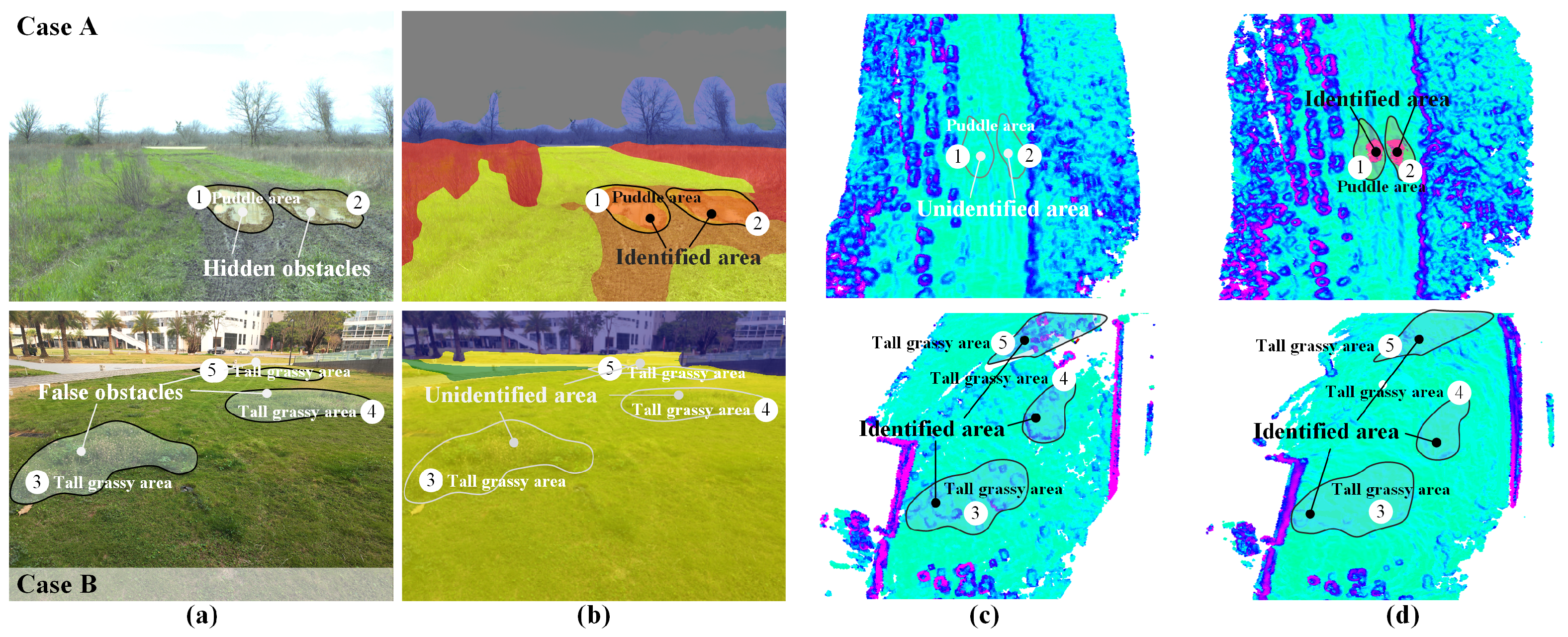
This section validates the proposed framework’s effectiveness with traversability mapping experiments in unstructured scenarios. The experiments employed the semantic segmentation network, GA-Nav, which incorporates the Group-wise Attention Mechanism (GAM) [36] for semantic segmentation. The traversability evaluation results of the proposed method in this paper are compared in Figure 4 for two an example scenarios. The results demonstrate the benefits of semantic and geometric fusion. In these cases, geometric computation fails to accurately identify certain types of areas (e.g., puddles), whereas the semantic segmentation method appears to identify tall vegetation as an impassable obstacle. Nevertheless, the combined visual and semantic approach proposed in this paper can precisely identify and evaluate both cases.
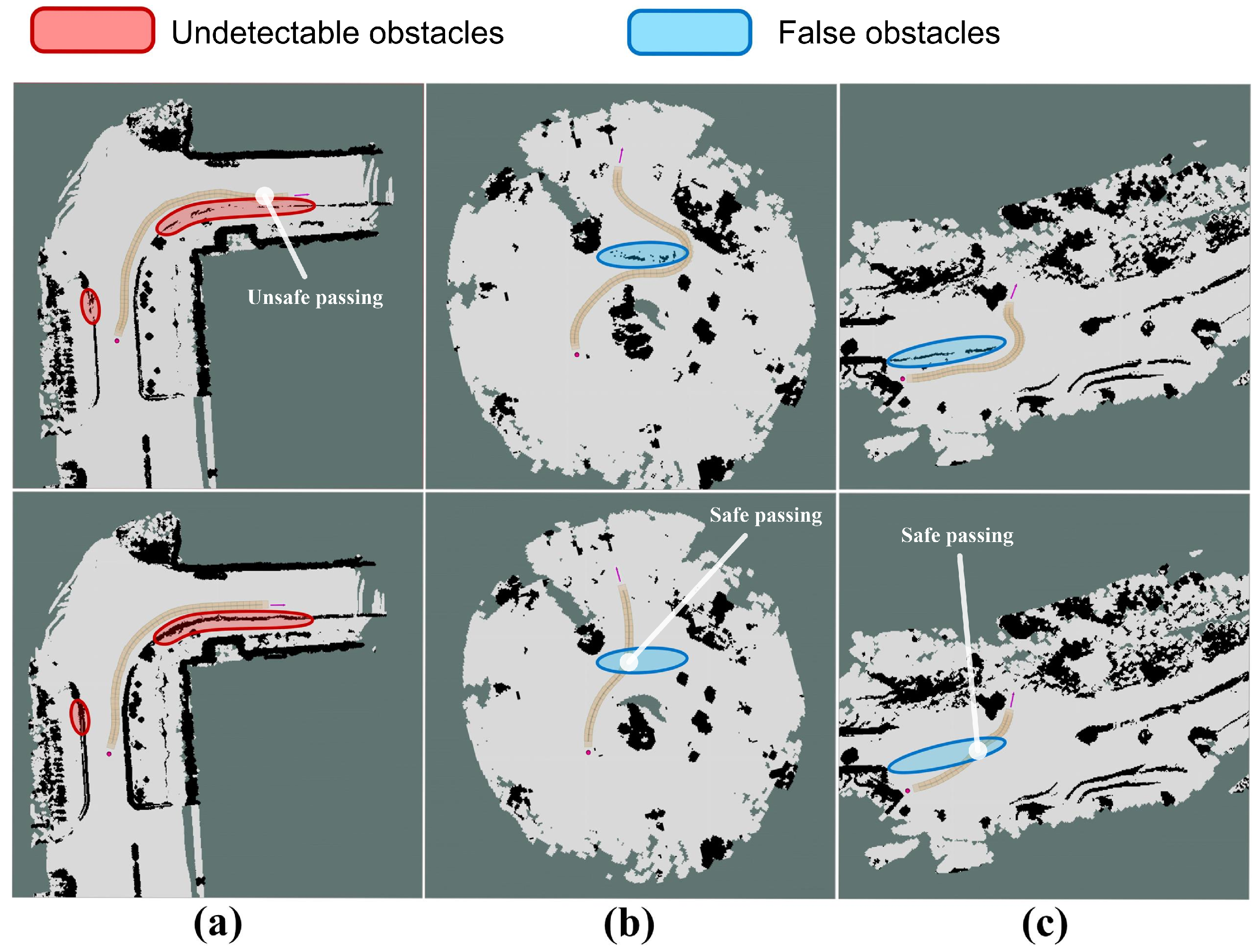
An occupancy grid map is created using the generated traversability map, to which an occupancy threshold of 0.65 is applied. Afterwards that, trajectory planning is carried out by randomly choosing the starting and ending places based on the occupancy map. These results of the autonomous navigation experiments in three scenarios are depicted in Figure 5. Despite being impassable, the radar blind red area in Scenario 1, which is a 15 cm raised shoulder, is erroneously categorized as passable by geometry-based approaches [30]. The geometric technique mistakenly classifies the blue high grass area in Scenarios 2 and 3, which is passable but obstructs radar detection, as impassable. By comparison, the proposed method precisely detects the red area as impassable in Scenario 1 and the blue areas as passable in Scenarios 2 and 3, as depicted in Figure 5.

4.2. Outdoor Navigation

The performance of the proposed navigation framework is assessed on different terrains around the university campus, including off-road terrains, sidewalks, and asphalt roads. The navigation performance of the proposed approach is compared with planners based on DWA (Dynamic Window Approach) [37], which uses velocity and direction adjustments based on motion capabilities and environment; BGK (Bayesian generalized kernel) [30], focusing on behavior kinematics and geometric planning for navigation; PUTN (Plane-fitting based Uneven Terrain Navigation) [38], constructing a probabilistic roadmap for pathfinding; and RSPMP (Real-time Semantic Perception and Motion Planning) [39], enhancing RRT with predefined motion sequences for efficient exploration. The following metrics are used to assess performance against these planners.
  • Success Rate: The proportion of trials in which the autonomous vehicle successfully traveled to its target without failing or colliding with obstacles.
  • Trajectory Roughness: The total of all vertical motion gradients encountered by the autonomous vehicle through its trajectory.
  • Normalized Trajectory Length: The ratio of the length of the navigation trajectory to the linear distance between the autonomous vehicle and the target point for all successful experiments.
  • Trajectories Selection: The ratio of the distance traveled by the autonomous vehicle on the most efficiently traversable surface to the total planned trajectory length.
  • Mean Velocity: The autonomous vehicle’s mean velocity while traversing various surfaces along the planned path.

4.3. Comparision and Analysis

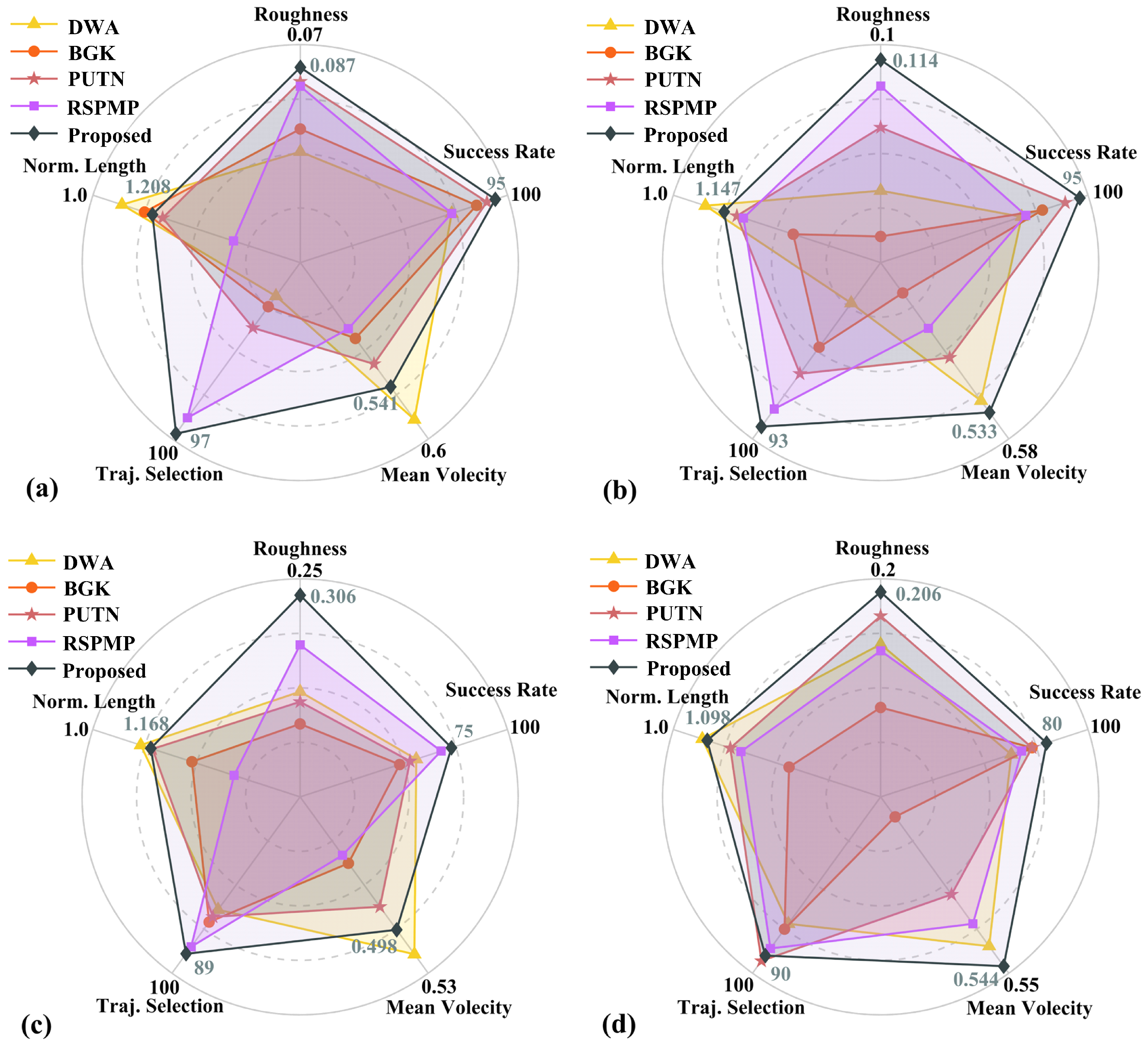
The performance of the navigation framework with the proposed approach is evaluated both qualitatively (Figure 6) and quantitatively (Table 1 and Figure 7) in four various off-road scenarios. It can be observed that in all scenarios, the proposed approach achieves the highest rate of success. Further, the autonomous vehicle obtains a decrease in trajectory roughness ranging from 5.1% to 35.8%. Additionally, the autonomous vehicle maintains a terrain surface selection accuracy of over 85% during the navigation process. Geometry-based methods such as DWA and BGK are susceptible to being affected by grass height (Scenario 2) or getting stuck in mud (Scenario 3), making it difficult to reach the goal. PUTN, which is based on plane fitting, is less affected by protruding weeds. Nevertheless, it still cannot distinguish the muddy surfaces and is prone to slipping (Scenario 3). In addition, other algorithms tend to follow shorter paths without considering path width, which increases the probability of collision (Scenario 4). The proposed method maximizes the probability of reaching the goal by prioritizing broader and lower-cost paths.
In terms of trajectory length, the proposed method plans a longer trajectory to avoid high-cost areas. However, due to the influence of the f d ξ i term in the local path evaluation function, the normalized length of the trajectory is still close to 1. In some scenarios, DWA and BGK generate shorter paths by directly moving toward the goal without considering surface changes when there are no obstacles.
The proposed method also outperforms other methods in all test scenarios on the metrics of trajectory roughness and trajectory selection, as it plans trajectories as much as possible on smooth and low-cost surfaces. RSPMP is closer to the proposed method for these two metrics, but it plans a steeper path at the endpoint of Scenario 2 due to not considering the surface slope information. BGK and PUTN only use elevation information to compute the cost map, without accounting for the semantic information, thus selecting rougher surfaces for trajectory planning.
With regard to the average velocity, it is evident that the proposed method consistently maintains an even speed for navigation in numerous scenarios. This is achieved by navigating on cost-efficient surfaces and avoiding any obstacles caused by wheel slipping or blocking. Conversely, BGK and PUTN are influenced by vegetation height easily, causing disorientation in their paths. They are also affected by muddy and slippery terrain, causing the autonomous vehicle to skid and reduce overall speed.
The experimental results show that the method proposed in this study has achieved significant improvements in key performance indicators. The success rate of the navigation algorithm was significantly improved from 4.4% to 13.6%, demonstrating its adaptability and effectiveness in complex outdoor environments. Meanwhile, the reduction in trajectory roughness ranged from 5.1% to 35.8%, which optimized the smoothness of navigation. In addition, the autonomous vehicle maintains a terrain surface selection accuracy of more than 85%, ensuring accurate decision making and reliable navigation.
Applying this paper’s methodology to a wide range of scenarios, computational and storage costs are not negligible. Therefore, future research needs to focus on designing more efficient data structures for unified terrain representation to enable terrain perception tasks over larger and more complex environments.
As shown in the attached Video S1 in Supplementary Materials, the proposed method achieves safe and reliable autonomous navigation in off-road terrain environments.

5. Conclusions

In this paper, a real-time terrain traversability method is proposed to generate accurate traversability maps for off-road navigation. It utilizes semantic features and Bayesian generalized kernel inference for dense elevation mapping. An efficient real-time terrain evaluation method is proposed that fuses semantic and geometric data, resulting in accurate traversability maps. The robustness and utility of the algorithm are demonstrated through UGV-based mapping and navigation in real-world scenarios. The focus of future research will be on the integration of deep learning and Bayesian approaches into semantic segmentation networks. This integration aims to more reliably estimate the uncertainty of semantic predictions and to incorporate semantic uncertainty into the mapping process, thereby increasing the reliability and accuracy of the map.

Supplementary Materials

The following supporting information can be downloaded at https://drive.google.com/file/d/1DL0KuJAfhP3YJU-ZrrpS5gR8SiMjQz_b/view?usp=sharing, Video S1: Experiment of Autonomous Vehicles Traversability Mapping Fusing Semantic-Geometric in Off-Road Navigation.

Author Contributions

All authors contributed to the study conception and design. Conceptualization and Supervision, B.Z., S.C. and C.X.; Methodology and Validation, W.C. and S.C.; Investigation and Software, C.X. and J.Q.; Writing—original draft, C.X. and W.C.; Writing—review & editing, B.Z., S.C. and W.C. All authors have read and agreed to the published version of the manuscript.

Funding

This research was funded by the National Natural Science Foundation of China (NSFC) (No. 62173234), the Shenzhen Science and Technology Program (No. 20220818095816035).

Data Availability Statement

All data generated or analysed during the study of this manuscript are included in the article.

Conflicts of Interest

With respect to the content of this paper, all the authors have no conflicts of interest to declare.

References

  1. Hornung, A.; Wurm, K.M.; Bennewitz, M.; Stachniss, C.; Burgard, W. OctoMap: An Efficient Probabilistic 3D Mapping Framework Based on Octrees. Auton. Robot. 2013, 34, 189–206. [Google Scholar] [CrossRef]
  2. Fankhauser, P.; Bloesch, M.; Gehring, C.; Hutter, M.; Siegwart, R. Robot-centric Elevation Mapping with Uncertainty Estimates. In Mobile Service Robotics; World Scientific: Poznań, Poland, 2014; pp. 433–440. [Google Scholar] [CrossRef]
  3. Ahtiainen, J.; Stoyanov, T.; Saarinen, J. Normal Distributions Transform Traversability Maps: LIDAR-Only Approach for Traversability Mapping in Outdoor Environments. J. Field Robot. 2017, 34, 600–621. [Google Scholar] [CrossRef]
  4. Zhang, B.; Li, G.; Zheng, Q.; Bai, X.; Ding, Y.; Khan, A. Path Planning for Wheeled Mobile Robot in Partially Known Uneven Terrain. Sensors 2022, 22, 5217. [Google Scholar] [CrossRef] [PubMed]
  5. Angelova, A.; Matthies, L.; Helmick, D.; Perona, P. Fast Terrain Classification Using Variable-Length Representation for Autonomous Navigation. In Proceedings of the 2007 IEEE Conference on Computer Vision and Pattern Recognition, Minneapolis, MN, USA, 17–22 June 2007; pp. 1–8. [Google Scholar] [CrossRef]
  6. Xie, E.; Wang, W.; Yu, Z.; Anandkumar, A.; Alvarez, J.M.; Luo, P. SegFormer: Simple and Efficient Design for Semantic Segmentation with Transformers. Adv. Neural Inf. Process. Syst. 2021, 34, 12077–12090. [Google Scholar] [CrossRef]
  7. Zhao, H.; Shi, J.; Qi, X.; Wang, X.; Jia, J. Pyramid Scene Parsing Network. In Proceedings of the 2017 IEEE Conference on Computer Vision and Pattern Recognition (CVPR), Los Alamitos, CA, USA, 21–26 July 2017; pp. 6230–6239. [Google Scholar] [CrossRef]
  8. Filitchkin, P.; Byl, K. Feature-based Terrain Classification for LittleDog. In Proceedings of the 2012 IEEE/RSJ International Conference on Intelligent Robots and Systems (IROS), Vilamoura-Algarve, Portugal, 7–12 October 2012; pp. 1387–1392. [Google Scholar] [CrossRef]
  9. Saucedo, M.A.; Patel, A.; Kanellakis, C.; Nikolakopoulos, G. Memory Enabled Segmentation of Terrain for Traversability Based Reactive Navigation. In Proceedings of the 2023 IEEE International Conference on Robotics and Biomimetics (ROBIO), Koh Samui, Thailand, 4–9 December 2023; pp. 1–6. [Google Scholar] [CrossRef]
  10. Gao, B.; Zhao, X.; Zhao, H. An Active and Contrastive Learning Framework for Fine-Grained Off-Road Semantic Segmentation. IEEE Trans. Intell. Transp. Syst. 2023, 24, 564–579. [Google Scholar] [CrossRef]
  11. Schilling, F.; Chen, X.; Folkesson, J.; Jensfelt, P. Geometric and Visual Terrain Classification for Autonomous Mobile Navigation. In Proceedings of the 2017 IEEE/RSJ International Conference on Intelligent Robots and Systems (IROS), Vancouver, BC, Canada, 24–28 September 2017; pp. 2678–2684. [Google Scholar] [CrossRef]
  12. Weerakoon, K.M.K.; Sathyamoorthy, A.J.; Patel, U.; Manocha, D. TERP: Reliable Planning in Uneven Outdoor Environments Using Deep Reinforcement Learning. In Proceedings of the 2022 International Conference on Robotics and Automation (ICRA), Philadelphia, PA, USA, 23–27 May 2022; pp. 9447–9453. [Google Scholar] [CrossRef]
  13. Ewen, P.; Li, A.; Chen, Y.; Hong, S.; Vasudevan, R. These Maps are Made for Walking: Real-Time Terrain Property Estimation for Mobile Robots. IEEE Robot. Autom. Lett. 2022, 7, 7083–7090. [Google Scholar] [CrossRef]
  14. Ewen, P.; Chen, H.; Chen, Y.; Li, A.; Bagali, A.; Gunjal, G.; Vasudevan, R. You’ve Got to Feel It to Believe It: Multi-Modal Bayesian Inference for Semantic and Property Prediction. arXiv 2024, arXiv:2402.05872. [Google Scholar]
  15. Ronneberger, O.; Fischer, P.; Brox, T. U-Net: Convolutional Networks for Biomedical Image Segmentation. In Medical Image Computing and Computer-Assisted Intervention—MICCAI 2015, Proceedings of the 18th International Conference, Munich, Germany, 5–9 October 2015; Springer: Cham, Switzerland, November 2015; pp. 234–241. [Google Scholar] [CrossRef]
  16. Alshawi, R.; Hoque, T.; Flanagin, M.C. A Depth-Wise Separable U-Net Architecture with Multiscale Filters to Detect Sinkholes. Remote Sens. 2023, 15, 1384. [Google Scholar] [CrossRef]
  17. Wellhausen, L.; Dosovitskiy, A.; Ranftl, R.; Walas, K.; Cadena, C.; Hutter, M. Where Should I Walk? Predicting Terrain Properties from Images via Self-supervised Learning. IEEE Robot. Autom. Lett. 2019, 4, 1509–1516. [Google Scholar] [CrossRef]
  18. Sathyamoorthy, A.J.; Weerakoon, K.M.K.; Guan, T.; Liang, J.; Manocha, D. TerraPN: Unstructured Terrain Navigation using Online Self-Supervised Learning. In Proceedings of the 2022 IEEE/RSJ International Conference on Intelligent Robots and Systems (IROS), Kyoto, Japan, 23–27 October 2022; pp. 7197–7204. [Google Scholar] [CrossRef]
  19. Wermelinger, M.; Fankhauser, P.; Diethelm, R.; Krüsi, P.; Siegwart, R.Y.; Hutter, M. Navigation Planning for Legged Robots in Challenging Terrain. In Proceedings of the 2016 IEEE/RSJ International Conference on Intelligent Robots and Systems (IROS), Daejeon, Republic of Korea, 9–14 October 2016; pp. 1184–1189. [Google Scholar] [CrossRef]
  20. Krusi, P.; Furgale, P.; Bosse, M.; Siegwart, R. Driving on Point Clouds: Motion Planning, Trajectory Optimization, and Terrain Assessment in Generic Nonplanar Environments. J. Field Robot. 2017, 34, 940–984. [Google Scholar] [CrossRef]
  21. Dixit, A.; Fan, D.D.; Otsu, K.; Dey, S.; Agha-Mohammadi, A.A.; Burdick, J.W. STEP: Stochastic Traversability Evaluation and Planning for Risk-Aware off-road Navigation; Results from the DARPA Subterranean Challenge. arXiv 2023, arXiv:2303.01614. [Google Scholar] [CrossRef]
  22. Chavez-Garcia, R.O.; Guzzi, J.; Gambardella, L.M.; Giusti, A. Learning Ground Traversability from Simulations. IEEE Robot. Autom. Lett. 2018, 3, 1695–1702. [Google Scholar] [CrossRef]
  23. Wellhausen, L.; Hutter, M. ArtPlanner: Robust Legged Robot Navigation in the Field. Field Robot. 2023, 3, 413–434. [Google Scholar] [CrossRef]
  24. Bozkurt, S.; Atik, M.E.; Duran, Z. Improving Aerial Targeting Precision: A Study on Point Cloud Semantic Segmentation with Advanced Deep Learning Algorithms. Drones 2024, 8, 376. [Google Scholar] [CrossRef]
  25. Qi, C.R.; Yi, L.; Su, H.; Guibas, L.J. PointNet++: Deep Hierarchical Feature Learning on point sets in a Metric Space. In Proceedings of the 31st International Conference on Neural Information Processing Systems, Long Beach, CA, USA, 4–9 December 2017; pp. 5105–5114. [Google Scholar] [CrossRef]
  26. Guan, T.; He, Z.; Song, R.; Manocha, D.; Zhang, L. TNS: Terrain Traversability Mapping and Navigation System for Autonomous Excavators. In Proceedings of the Robotics: Science and Systems XVIII, New York, NY, USA, 27 June–1 July 2022. [Google Scholar] [CrossRef]
  27. Siva, S.; Wigness, M.B.; Rogers, J.G. Robot Adaptation to Unstructured Terrains by Joint Representation and Apprenticeship Learning. In Proceedings of the Robotics: Science and Systems XV, Freiburg im Breisgau, Germany, 22–26 June 2019. [Google Scholar] [CrossRef]
  28. Kahn, G.; Abbeel, P.; Levine, S. LaND: Learning to Navigate from Disengagements. IEEE Robot. Autom. Lett. 2021, 6, 1872–1879. [Google Scholar] [CrossRef]
  29. Gregory, K.; Pieter, A.; Sergey, L. Badgr: An autonomous Self-supervised Learning-Based Navigation System. IEEE Robot. Autom. Lett. 2021, 6, 1312–1319. [Google Scholar] [CrossRef]
  30. Shan, T.; Wang, J.; Englot, B.; Doherty, K.A.J. Bayesian Generalized Kernel Inference for Terrain Traversability Mapping. In Proceedings of the Conference on Robot Learning, PMLR, Zürich, Switzerland, 29–31 October 2018; pp. 829–838. [Google Scholar]
  31. Vega-Brown, W.; Doniec, M.; Roy, N. Nonparametric Bayesian Inference on Multivariate Exponential Families. Adv. Neural Inf. Process. Syst. 2014, 27, 2546–2554. [Google Scholar] [CrossRef]
  32. Bellone, M.; Messina, A.; Reina, G. A New Approach for Terrain Analysis in Mobile Robot Applications. In Proceedings of the 2013 IEEE International Conference on Mechatronics (ICM), Vicenza, Italy, 27 February–1 March 2013; pp. 225–230. [Google Scholar] [CrossRef]
  33. Gammell, J.D.; Srinivasa, S.S.; Barfoot, T.D. Informed RRT*: Optimal Sampling-based Path Planning Focused via Direct Sampling of an Admissible Ellipsoidal Heuristic. In Proceedings of the 2014 IEEE/RSJ International Conference on Intelligent Robots and Systems (IROS), Chicago, IL, USA, 14–18 September 2014; pp. 2997–3004. [Google Scholar] [CrossRef]
  34. Scout-2.0. Available online: https://iqr-robot.com/product/agilex-scout-2-0/ (accessed on 17 August 2024).
  35. Wei, X.; Yixi, C.; Dongjiao, H.; Jiarong, L.; Fu, Z. Fast-lio2: Fast Direct Lidar-inertial Odometry. IEEE Trans. Robot. 2022, 38, 2053–2073. [Google Scholar] [CrossRef]
  36. Guan, T.; Kothandaraman, D.; Chandra, R.; Sathyamoorthy, A.J.; Weerakoon, K.; Manocha, D. GA-Nav: Efficient Terrain Segmentation for Robot Navigation in Unstructured Outdoor Environments. IEEE Robot. Autom. Lett. 2022, 7, 8138–8145. [Google Scholar] [CrossRef]
  37. Fox, D.; Burgard, W.; Thrun, S. The Dynamic Window Approach to Collision Avoidance. IEEE Robot. Autom. Mag. 1997, 4, 23–33. [Google Scholar] [CrossRef]
  38. Jian, Z.; Lu, Z.R.; Zhou, X.; Lan, B.; Xiao, A.; Wang, X.; Liang, B. PUTN: A Plane-fitting Based Uneven Terrain Navigation Framework. In Proceedings of the 2022 IEEE/RSJ International Conference on Intelligent Robots and Systems (IROS), Shanghai, China, 23–27 October 2022; pp. 7160–7166. [Google Scholar] [CrossRef]
  39. Chen, D.; Zhuang, M.; Zhong, X.; Wu, W.; Liu, Q. RSPMP: Real-time Semantic Perception and Motion Planning for Autonomous Navigation of Unmanned Ground vehicle in off-road environments. Appl. Intell. 2023, 53, 4979–4995. [Google Scholar] [CrossRef]
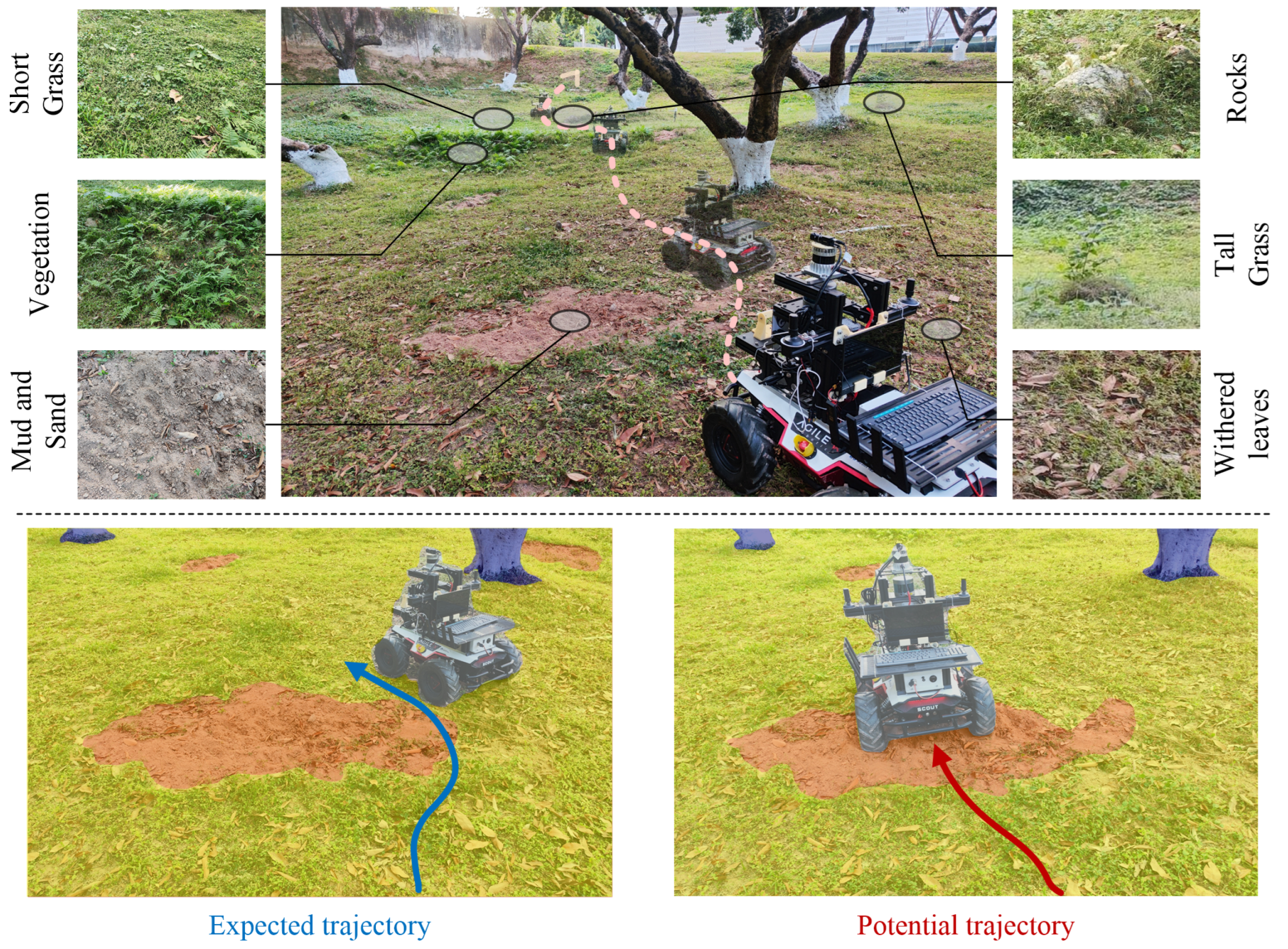
Figure 1. Navigation of an autonomous vehicle in unstructured wild environments with different terrains and obstacles.
Drones 08 00496 g001
Figure 2. Autonomous navigation framework overview. The algorithm evaluates terrain traversability using RGB images and 3D point clouds. The traversability map guarantees safe and smooth path planning.
Drones 08 00496 g002
Figure 3. Semantic cost projection. Some examples of projection: green represents easily traversable areas such as asphalt and concrete, yellow represents rough surfaces such as grass and sand, orange represents rocks, and blue represents obstacles.
Drones 08 00496 g003
Figure 4. Comparison of obstacle identification results of the three methods in two real-world scenarios. In the scenario, Case A (first row) has two hidden obstacle areas (two puddle areas 1, 2); Case B (second row) has three false obstacles (three individual tall grassy areas 3, 4, and 5). (a) RGB image inputs (corresponding to the two images in the first column) for both cases; (b) semantic segmentation for both cases; (c) geometric gridmaps for both cases; (d) fused passivity maps for both cases.
Drones 08 00496 g004
Figure 5. Results of evaluating the terrain for geometry only (top) and geometric-semantic fusion (bottom). (a) Scenario 1, (b) Scenario 2, and (c) Scenario 3. The areas that the geometric method gets wrong are shown in blue, and the areas where the geometry is neglected are displayed in red.
Drones 08 00496 g005
Figure 6. Autonomous vehicle trajectories when navigating in four various unstructured scenarios using proposed method (black), RSPMP (blue), PUTN (red), BGK (orange), and DWA (yellow). (a) Scenario 1; (b) Scenario 2; (c) Scenario 3; (d) Scenario 4. It can be observed that proposed method allows the autonomous vehicle to navigate on smooth, low-cost surfaces and maintains a short trajectory.
Drones 08 00496 g006
Figure 7. Quantitative comparison of navigation performance between various methods. (a) Scenario 1; (b) Scenario 2; (c) Scenario 3; (d) Scenario 4.
Drones 08 00496 g007
Table 1. Navigation performance of the proposed method compared with other methods in four various scenarios.
MetricsMethodScenario 1Scenario 2Scenario 3Scenario 4
Success Rate (%)DWA75705565
BGK85805075
PUTN90905575
RSPMP75707070
Proposed95957580
Traj. RoughnessDWA0.1830.2340.6380.230
BGK0.1590.2760.7490.259
PUTN0.1390.1760.6730.217
RSPMP0.1140.1380.4770.233
Proposed0.0870.1140.3060.206
Norm. Traj. LengthDWA1.1271.0931.1391.084
BGK1.1871.3471.2871.335
PUTN1.2351.1841.1731.165
RSPMP1.4231.2031.4091.196
Proposed1.2081.1471.1681.098
Traj. Selection (%)DWA19236472
BGK25487175
PUTN37636893
RSPMP88838586
Proposed97938990
Mean VelocityDWA0.5780.5410.5160.527
BGK0.4860.4310.4490.417
PUTN0.5150.4970.4810.483
RSPMP0.4750.4670.4430.508
Proposed0.5410.5530.4980.544
Disclaimer/Publisher’s Note: The statements, opinions and data contained in all publications are solely those of the individual author(s) and contributor(s) and not of MDPI and/or the editor(s). MDPI and/or the editor(s) disclaim responsibility for any injury to people or property resulting from any ideas, methods, instructions or products referred to in the content.