Olive Tree Segmentation from UAV Imagery

Abstract

This paper addresses the challenge of olive tree segmentation using drone imagery, which is crucial for precision agriculture applications. We tackle the data scarcity issue by augmenting existing detection datasets. Additionally, lightweight model variations of state-of-the-art models like YOLOv8n, RepViT-SAM, and EdgeSAM are combined into two proposed pipelines to meet computational constraints while maintaining segmentation accuracy. Our multifaceted approach successfully achieves an equilibrium among model size, inference time, and accuracy, thereby facilitating efficient olive tree segmentation in precision agriculture scenarios with constrained datasets. Following comprehensive evaluations, YOLOv8n appears to surpass the other models in terms of inference time and accuracy, albeit necessitating a more intricate fine-tuning procedure. Conversely, SAM-based pipelines provide a significantly more streamlined fine-tuning process, compatible with existing detection datasets for olive trees. However, this convenience incurs the disadvantages of a more elaborate inference architecture that relies on dual models, consequently yielding lower performance metrics and prolonged inference durations.

1. Introduction

In the era of intense environmental pollution and draining of resources worldwide, the availability of sufficient and high-quality food supplies is greatly threatened, while over-cultivation combined with the excessive use of chemicals, as either fertilizers or pesticides, even endanger food safety. As a noble alternative, organic farming promotes sustainable and environmentally friendly agricultural practices. Organic farming methods prioritize the use of natural processes and avoid synthetic chemicals, pesticides, and fertilizers. This helps reduce the environmental impact associated with conventional farming, including soil and water pollution. Moreover, organic farming avoids the use of synthetic pesticides and herbicides, which can have negative effects on human health. Choosing organic products can help reduce the risk of exposure to potentially harmful chemicals in food. In addition, organic farming benefits water conservation.

Olive cultivation plays a crucial role in numerous economies worldwide, requiring efficient management practices for optimal yield and sustainability. Olive oil production has been greatly affected by climate change in recent years, which was experienced intensely in major European olive-producing countries, like Spain, Italy and Greece. High temperatures and droughts negatively affect the quantity and quality of yields worldwide for various crop types [1]. In particular, for olive trees, the effects of a high-temperature environment are genotype dependent and, in general, high temperatures during fruit development affect the following three important traits: fruit weight, oil concentration and oil quality in a cultivar-dependent manner [2]. The combination of the prolonged drought and absence of rain result in the soil being dried out and the olive trees deprived of any water source and the growers of a substantial crop.

On the other hand, olive fruit fly development is favored by the lack of heat waves and rain. The olive fruit fly (scientific name: “Bactrocera oleae” or “Dacus oleae (Gmelin)”) is a major concern for olive tree cultivation, causing serious damage to the olive fruit, significantly affecting both the quantity and quality of yields [3]. Kaolin clay or spinosad-based bait are often used for olive fruit fly control as an organic treatment and have been used to protect plants from various insect and pests, achieving protection against total and harmful fly infestation [4].

Traditionally, olive tree care involves manual methods, which are time-consuming, labor-intensive, and prone to human error [5]. Precision spraying allows for the targeted application of pesticides and fertilizers, minimizing the waste and environmental impact [6]. Unmanned Aerial Vehicles (UAVs) are already widely used in precision agriculture, offering rapid and detailed data collection capabilities [7,8] and field monitoring using captured images. Leveraging UAV capabilities and machine learning-based innovations, autonomous precision spraying may lead to a good balance between organic olive yield quantity, quality, and costs through collaborative intelligent systems.

Precision spraying involves the extraction and analysis of drone imagery in real time, which poses multiple challenges, including variable lighting conditions, overwhelming data volumes, and background clutter [5,9]. Analysis of drone imagery via olive tree segmentation has attracted research interest [10] as an automated, efficient process for identifying and delineating individual olive trees within a captured image. The advantages of olive tree segmentation include rapid data analysis, timely decision making for agricultural management, and enhanced monitoring and maintenance of olive groves. Hence, the segmentation procedure facilitates tree health monitoring by enabling early identification of unhealthy or diseased trees, leading to prompt intervention and improved crop yield [11,12]. Furthermore, accurate tree counts and segmentations pave the way for the development of automated yield estimation systems [13,14].

In fact, segmentation of olive trees addressing real-time constraints addresses highly automated precision agriculture use cases delivered in the IoT, edge, and cloud continuum through meta-operating systems (metaOS). MetaOS provide hardware abstraction, device control, service orchestration, and management across diverse IoT, edge, and cloud resources, effectively enabling AI and other service delivery through edge and cloud computing and 6G communications, also integrating IoT systems. Notable research and innovation actions suggest flexible and coherent orchestration of services across nodes [15,16,17], whether they belong to cloud, edge, or the IoT side, as well as integration of edge devices such as UAVs [18,19] in the continuum. Such kind of meta-OS suggest flexible allocation of services in the dynamically changing resource environment, exploiting resources available in the continuum.

Within the metaOS vision, AI service delivery on edge devices is still challenging in real-world cases and is generally applied in isolated scenarios constrained by limited resources. One of the most significant hurdles in achieving real-time on-device olive tree segmentation lies in the computational limitations of these aerial platforms. Unlike powerful workstations used for training deep learning models, drones possess limited processing power, memory, and battery life. This necessitates a shift toward inference, the process of running a trained model on new data, being performed efficiently in the resource-constrained environment of the drone. Traditional, complex deep learning models, while highly accurate, often consist of architectures with millions of parameters. Executing these models on drones is challenging due to the limited processing power that hinders real-time performance. Additionally, drones have restricted onboard memory, which limits the size of the models that can be stored. The impracticality of processing large amounts of data during flight necessitates the development of models that require minimal memory. Furthermore, real-time processing demands substantial continuous power consumption. Complex models can deplete drone batteries quickly, reducing the flight duration and limiting the area covered during the segmentation task. For all of the above-mentioned reasons, the present work studies lightweight AI models for olive tree segmentation using drone images, which will support on-device segmentation on far edge devices (UAVs) in the context of service delivery in the continuum.

A major challenge that arises when dealing with the task of training olive tree segmentation models using drone imagery is the lack of available public data that are necessary to train or fine-tune the deep learning models that perform segmentation. Even for state-of-the-art (SOTA) models, each segmentation task requires some form of retraining so that the model can capture the desired information. This process requires a large amount of labeled training data, which, in this case, means drone images of olive trees with segmentation masks for each olive tree. To the best of our knowledge, public segmentation and detection datasets are very limited.

These challenges underscore the necessity for innovative approaches that tackle the intricacies of olive tree segmentation, overcoming the data scarcity problem while respecting the strict computational limitations in drone applications. To overcome these challenges, we propose two distinct methodologies for training segmentation models that bypass the scarcity of training data, providing time- and cost-effective alternatives to manual annotation by leveraging existing, limited detection datasets. We also focus our research on lightweight versions of state-of-the-art (SOTA) segmentation models, such as YOLOv8 [20] and SAM [21], which would be appropriate for test and deployment in resource-constrained environments, such as drones, for real-time segmentation in future work. To the best of our knowledge, a comparative analysis of alternative methods for olive tree segmentation on limited publicly available data has not been conducted before. Aiming to address the aforementioned challenges, the paper presents the following contributions:

• Tackles the data scarcity problem associated with olive tree segmentation using drone images by introducing a methodology for creating a custom annotated segmentation dataset specifically tailored for olive tree segmentation;
• Details the steps of the methodology to reproduce the custom annotated segmentation dataset based on the publicly available detection dataset;
• Overcomes the need for manual annotation, which requires a lot of human labor;
• Introduces two olive tree segmentation pipelines that utilize lightweight versions of SOTA models and focus on both accuracy and inference time, making them suitable for potential on-device deployment.

2. Related Work

This section delves into the existing literature related to (1) image segmentation methods, particularly focusing on tree segmentation and specific works on olive tree segmentation, and (2) lightweight AI models for segmentation.

2.1. State-of-the-Art Segmentation Methods

Image segmentation plays a crucial role in various computer vision applications, including object detection, image understanding, and scene analysis. Deep learning models have revolutionized the field, achieving remarkable advancements in segmentation accuracy and performance. We explore relevant research within this domain, focusing on tree segmentation and specific olive tree segmentation efforts.

Deep learning architectures completely transformed the field of image segmentation, achieving impressive results in accurately delineating objects within images. Introduced by Long [22], fully convolutional networks (FCNs) revolutionized image segmentation by demonstrating that fully convolutional architectures, unlike traditional approaches with classification layers, can effectively perform pixel-wise labeling. This breakthrough paved the way for significant advancements in the field. Variants like U-Net [23] further improved segmentation performance by incorporating skip connections. These connections directly combine low-level feature maps from the encoder with high-level semantic information from the decoder, allowing the network to capture both fine-grained details and the global context. Moreover, DeepLabv3 [24] introduced another innovation, namely, atrous convolutions. These convolutions enable the network to capture features at different scales without increasing the number of parameters, leading to improved segmentation accuracy, especially for tasks requiring precise object boundary delineation. One prominent approach involves semantic networks, which aim to classify each pixel in an image into a specific semantic category. This allows for the identification and precise delineation of objects within the scene.

Popular examples include DeepLabV3+ [25], which builds upon DeepLabv3 by leveraging spatial pyramid pooling (SPP). SPP aggregates features from different scales within the image, allowing the network to capture multiscale information and improve segmentation accuracy for objects of varying sizes. Another prominent example is PSPNet [26], which incorporates a pyramid pooling module to achieve similar multiscale feature extraction capabilities, leading to more robust segmentation performance. Another powerful approach utilizes encoder–decoder architectures. These architectures typically consist of the following two main components: an encoder that extracts image features and a decoder that up-samples and refines the extracted features to produce the final segmentation output. SegNet [27] is a notable example of this architecture. It utilizes encoders pretrained on image classification tasks and builds upon them with decoders that perform up-sampling and feature concatenation. U-Net++ [28] further refines the U-Net architecture by introducing more complex skip connections and decoder blocks. These enhancements allow U-Net++ to capture richer feature information at different levels, leading to improved segmentation performance compared to the original U-Net.

Additionally, Mask R-CNN [29] leverages an encoder–decoder structure to achieve outstanding performance in object segmentation tasks. The key innovation of Mask R-CNN lies in its ability to perform pixel-wise instance segmentation alongside object detection. This is achieved through the addition of an extra mask prediction branch. State-of-the-art advancements have further expanded the capabilities of image segmentation. Recent object detection frameworks, like You Only Look Once (YOLO) v8 [20], can not only identify objects within an image but also provide pixel-wise segmentation masks through techniques like bounding box to segmentation mask conversion. This enables the efficient identification and delineation of objects. YOLOv8 comes in various pretrained model sizes, each offering a trade-off between accuracy and speed. The nano version is the smallest and fastest YOLOv8 model, designed specifically for deployment on mobile devices and resource-constrained environments. While offering the quickest inference speed, it may have a slightly lower accuracy compared to larger models. It comes with only 3.2 M parameters, compared to the 68.2 M of the x version, the larger model of the YOLOv8 series, and reported a difference in processing times of 6 times. Additionally, Meta’s Segment Anything Model (SAM) [21] presents a unique approach using prompt-based learning. By allowing users to specify the desired segmentation task through textual prompts, SAM offers remarkable flexibility for various segmentation scenarios, including object and part segmentation.

2.2. Tree Segmentation

Research on tree segmentation has gained significant traction due to its numerous applications in forestry, agriculture, and environmental monitoring. Several studies have explored various deep learning approaches for this task. The authors of [30] propose an improved approach for individual tree segmentation in aerial imagery based on the Mask R-CNN, a popular deep learning architecture for object detection and instance segmentation. Their work highlights the potential of deep learning models to achieve accurate segmentation of individual tree crowns, which is crucial for tasks like tree counting and biomass estimation. Furthermore, the authors of [31] suggest a two-stage deep learning framework for tree crown segmentation in high-resolution satellite images. Their approach demonstrates the effectiveness of incorporating both spatial features extracted from the image itself and contextual information from surrounding pixels. By combining these elements, the model can achieve more accurate segmentation, especially in areas with dense vegetation or overlapping tree crowns. Moreover, in [32] a two-stage convolutional neural network (TS-CNN) approach is proposed, specifically designed for the large-scale detection of oil palm trees in high-resolution satellite images. The TS-CNN consists of the following two separate CNNs: one for land cover classification (identifying different types of ground cover, like forest or water) and another for object classification (detecting oil palm trees within the classified land cover). This two-stage approach allows the network to focus on relevant regions within the image and achieve efficient and accurate oil palm tree detection. In addition, the authors of [33] present a deep learning model specifically tailored for segmenting individual trees in urban environments using street-level imagery. Urban environments pose unique challenges for tree segmentation due to complex backgrounds, cluttered scenes, and overlapping foliage. These challenges are addressed in [33] by developing a model that can effectively distinguish individual trees from their surroundings, making it valuable for applications like urban forest management and street tree health monitoring.

2.3. Olive Tree Segmentation

While research on tree segmentation is extensive, studies that specifically focus on olive trees are still emerging. The use of Mask R-CNN is investigated in [10] for olive tree crown and shadow segmentation in UAV images. The study demonstrates the potential of deep learning models for the effective segmentation of olive trees, even when relying on limited datasets. Moreover, the authors of [34] explore the application of deep learning for olive tree detection and counting in satellite imagery. While not directly focused on segmentation, their work highlights the potential of deep learning methods for analyzing olive trees in remote sensing applications.

2.4. Lightweight AI Models for Segmentation

To overcome the limitations of traditional deep learning models on drones, researchers have focused on developing lightweight versions of state-of-the-art models, prioritizing the principles of reduced model complexity, efficient operations, and knowledge distillation. Through streamlined architectures with fewer layers and parameters, leading to smaller model footprints and lower computational demands, they achieve reduced model complexity. Techniques like pruning and quantization can further reduce the model size and enhance efficiency [35]. Additionally, efficient operations like depth-wise separable convolutions become crucial, achieving comparable accuracy with traditional convolutions while requiring fewer computations [36,37]. Finally, knowledge distillation techniques can transfer knowledge from a pretrained, complex model to a smaller model, allowing the lightweight model to retain high accuracy despite its reduced size [38,39]. By implementing these approaches, researchers are developing lightweight versions of popular deep learning models, like U-Net [23], SAM [21], and YOLOv8, specifically tailored for real-time segmentation tasks on drones.

Beyond the development of lightweight versions of SOTA models, deploying deep learning models on resource-constrained platforms like drones necessitates exploring real-time segmentation techniques optimized for edge devices. Recent research has made significant strides in this domain.

Traditional deep learning models often consist of complex architectures with millions of parameters, hindering their deployment on devices with limited processing power. Researchers have focused on developing lightweight models specifically designed for real-time applications. MobileNet [36] achieves impressive accuracy with minimal computational overhead by utilizing depth-wise separable convolutions. Traditional convolutions involve processing all channels of an input feature map at once. Depth-wise separable convolutions break this process down into the following two steps: a depth-wise convolution that applies filters to each channel independently, followed by a pointwise convolution that combines the filtered channels. This approach significantly reduces the number of computations required while maintaining similar accuracy compared to traditional convolutions. EfficientNet [40] utilizes a compound scaling technique to achieve a good balance between accuracy and efficiency. Compound scaling scales all aspects of the network architecture (depth, width, and resolution) proportionally, maintaining the balance among these factors that contributes to the model’s performance. This approach allows EfficientNet models to achieve high accuracy on par with complex models while maintaining a smaller footprint and faster inference times, making them suitable for real-time applications on edge devices.

Another technique, knowledge distillation, introduced in [38], involves transferring knowledge from a pretrained, possibly complex model to a smaller, lightweight model. The pretrained model, often trained on a massive dataset, has already learned rich feature representations from the data. To the best of our knowledge, it is the first work that presents two pipelines for olive tree segmentation on available data. This makes knowledge distillation a powerful tool for deploying accurate deep learning models on resource-constrained devices. Offloading some processing tasks to edge devices like ground stations or cloud platforms can alleviate the computational burden on the drone itself [41]. By strategically distributing the workload between the drone and edge devices, real-time performance can be maintained while enabling the application of more powerful models for segmentation tasks. This approach can be particularly beneficial for complex tasks that require high accuracy or involve processing large amounts of data.

3. Olive Tree Segmentation Methodology

This research delves into the challenges of olive tree segmentation using drone images by utilizing lightweight AI models. A significant hurdle in this endeavor is the limited availability of publicly accessible, high-quality olive tree segmentation datasets. To address this data scarcity, we adopted a multipronged approach.

Firstly, three existing public datasets related to olive trees detection and segmentation, although small, were leveraged. To artificially expand the dataset and combat potential overfitting during model training, a set of basic data augmentation techniques were implemented. These techniques involve rotations, flips, and scaling of existing images. These variations enrich the dataset and improve model generalizability. Subsequently, these augmented datasets were merged into a single, more extensive resource for training purposes.

Next, different lightweight segmentation approaches were explored to identify the most suitable model for olive tree segmentation using drone images. This involved employing two distinct segmentation foundation models, namely, YOLOv8 and SAM. These models were chosen based on the following two key criteria: their performance in achieving high segmentation accuracy on similar tasks, and their efficiency in terms of being optimized and adapted to the limited computational resources of drones.

Following these explorations, a custom annotated segmentation dataset specifically tailored for these applications was created. This dataset is crucial for fine-tuning the models and ensuring their optimal performance on drone images. The creation of this custom dataset is informed by the insights and results obtained from the combined models used in the previous ensemble learning step. Finally, to optimize the models for drone images of olive trees, YOLOv8-seg model, a variant of YOLOv8 series optimized for segmentation, is fine-tuned on the newly created, custom-annotated olive tree segmentation dataset. This fine-tuning process essentially adjusts the internal parameters of the models to better handle the specific task and data characteristics associated with olive tree segmentation using drone imagery.

A crucial aspect of this research involves a comprehensive evaluation focusing on the inference time of each proposed methodology. This evaluation allowed for the identification of the model combination and approach that delivers the most accurate segmentation results while maintaining computational efficiency. This balance between accuracy and computational efficiency is paramount for successful real-world applications of olive tree segmentation in precision agriculture. By implementing this multifaceted approach, the data scarcity challenge was overcome, different segmentation strategies were explored, and, ultimately, the optimal methodology for olive tree segmentation using drone images in practical agricultural settings was identified.

The primary challenge in the task is to perform instance segmentation on olive trees on drone images, necessitating a careful balance between model size, inference time, and accuracy. Although state-of-the-art models like the SAM and YOLOv8x, the larger model of the YOLOv8 series, excel in performance, their deployment on edge devices, such as drones, is hindered by computational resource limitations. To address this, lightweight model variations are considered to deliver commendable results with significantly reduced inference times at the expense of reduced accuracy. Indicatively, MobileSAM [42] introduces the use of TinyViT [43] to replace the heavy image encoder, reducing parameters from 615 M to 9.66 M and cutting inference time by nearly 40 times on a single GPU. Despite this improvement, deployment on resource-constrained edge devices encounters challenges due to the memory and computational overheads associated with self-attention mechanisms.

Considering the resource constraints, two distinct approaches are explored, employing RepViT-SAM [44] and YOLOv8n, the smaller model of the YOLOv8 series. The reason that the YOLOv8 series, and not some later YOLO version, is chosen is that it is the latest stable series that offers a nano version. Both approaches propose a pipeline that combines these models in different orders, with each approach tailored to specific considerations, namely, data availability and optimization of inference time for possible deployment on edge devices, such as drones. The main contribution of this work lies in overcoming data scarcity challenges in olive tree segmentation from drone images by adopting a multipronged approach that includes dataset augmentation, exploration of segmentation models, creation of a custom annotated dataset, and fine-tuning for olive tree drone imagery, ultimately identifying the optimal methodology balancing accuracy and computational efficiency for practical agricultural settings.

3.1. RepViT-SAM/EdgeSAM for Segmentation Methodology

RepViT-SAM [44] takes a step further than SAM by replacing the image encoder with RepViT [45], achieving a superior performance to MobileSAM, with nearly ten times the inference speed. RepViT utilizes several techniques to achieve efficiency, including multiscale convolutional layers and bottleneck design with residual connections. These techniques help to reduce the number of computations required while preserving feature quality. On the other hand, EdgeSAM [46] leverages a new technique called “prompt-in-the-loop distillation”. This approach incorporates both the prompt encoder and mask decoder used in generating segmentation masks during the distillation process. This ensures the distilled model effectively captures the intricate relationship between user prompts and the resulting segmentation masks. Compared to the original SAM, EdgeSAM achieves a 40-fold speed increase, making it suitable for potential real-time applications on resource-constrained devices, while maintaining competitive segmentation accuracy compared to MobileSAM.

RepViT-SAM and EdgeSAM are designed to work in a zero-shot learning setting, meaning they can handle unseen classes during segmentation. While this is advantageous for versatility, it presents a hurdle in this specific scenario of on-device segmentation on olive trees running on a drone. Both SAM variants require bounding boxes as input to predict segmentation masks. However, they cannot inherently identify the class of objects within those bounding boxes. In the case of olive tree segmentation, RepViT-SAM/EdgeSAM would not be able to distinguish olive trees from other objects in the image on its own. To address this limitation, the proposed approach, depicted in Figure 1, suggests a pipeline that combines YOLOv8n-det, a variant of the YOLOv8 series optimized for object detection, with RepViT-SAM/EdgeSAM for segmentation. However, this introduces additional complexity since it relies upon these two models for inference. Also, YOLOv8n-det, in its pretrained form, is not equipped to recognize “olive trees” or even the broader category of “trees”. To make the pipeline function effectively, the YOLOv8n-det model would require fine-tuning. Since olive tree detection datasets are publicly available, this step is straightforward. This process involves retraining the model with a detection dataset specifically for olive trees. The fine-tuned YOLOv8n-det would then be able to provide bounding boxes specifically for olive trees, which RepViT-SAM/EdgeSAM could subsequently use for segmentation. Overall, while SAM variants offer zero-shot segmentation capabilities, their class-agnostic nature necessitates a more complex pipeline for olive tree segmentation. The pipeline’s reliance on a fine-tuned YOLOv8n-det model adds an extra step to the process.

3.2. YOLOv8n-Seg for Segmentation Methodology

YOLOv8 builds upon its predecessors with innovations like anchor-free detection and the focus mechanism for improved accuracy. Unlike previous YOLO versions that relied on predefined anchor boxes, YOLOv8 takes a different approach. It directly predicts the bounding box center coordinates and objectness confidence score (a measure of the probability that an object exists in a proposed region of interest), eliminating the need for anchor boxes and simplifying the detection process. YOLOv8 introduces a novel focus layer that enhances the model’s ability to focus on salient regions of the input image during training. This improves object detection accuracy, especially for smaller objects within the image. Finally, it incorporates a path aggregation network (PAN) structure that facilitates better feature fusion across different scales within the network. This allows the model to effectively combine high-resolution features for precise localization with low-resolution features that capture broader contextual information.

The proposed approach simplifies the segmentation process, as can be seen in Figure 2, by relying solely on a single model, the YOLOv8 segmentation model (YOLOv8-seg). YOLOv8-seg handles both object detection and segmentation tasks simultaneously, unlike the first approach that combines YOLOv8n-det for detection and RepViT-SAM for segmentation. Thus, it provides a much simpler inference procedure. Similarly to the first approach, it needs fine-tuning, since the pretrained YOLOv8-seg model cannot inherently recognize olive trees, as its training dataset did not contain this type of imagery. To enable olive tree segmentation on this pipeline, fine-tuning is required using a segmentation dataset containing images of olive trees. As there is a lack of a public olive tree segmentation dataset, the creation of a custom dataset leveraging the available resources is proposed. Since RepViT-SAM can perform segmentation, although it is class-agnostic, it is employed to generate segmentation masks for the images in an open-source olive tree detection dataset. The corresponding bounding boxes from the dataset are used to guide the segmentation process. Preprocessing is performed to transform the masks into the appropriate format. The YOLO-compatible masks are then used for YOLOv8-seg fine-tuning.

3.3. Methods Comparison Methodology

To systematically assess and compare the performance of the two proposed methods for olive tree segmentation using drone images, namely, the YOLOv8-Seg approach and the SAM-based approach, a robust comparison framework is essential. This section outlines the methodology for conducting this comparison, which focuses on several key dimensions, as follows: computational efficiency, accuracy, and practical deployment feasibility. To ensure consistency in evaluation, the same datasets across all methods are used, the models are evaluated on identical hardware configurations to standardize the comparison, and a consistent software environment, PyTorch, for all model implementations and evaluations is used. The comparison is based on the performance metrics, which are further described in Section 4.2, the inference time, and the complexity of each approach. Complexity is defined as the reliance of each approach on multiple models in the two different stages of the process, named fine-tuning and inference.

The process of comparing the two proposed methodologies using different dataset setups remained the same for both approaches, as shown in Figure 3. This consistency ensures that the experiments are uniform, allowing for comparable results. The user first preprocesses the datasets by downloading the images for each dataset, splitting each one into training, validation, and test sets following the 70-15-15 rule and merging them if needed. Details on the datasets are presented in Section 4.1. Then, the user can choose to fine-tune either the YOLOv8-based method or the SAM-based methods on the training data and use the fine-tuned model for inference on the test data, the fine-tuning and inference processes are further discussed in Section 4.4 and Section 4.5 Finally, the models are evaluated based on the evaluation metrics, the inference time, and the complexity of each approach, and based on the comparison the final decision is made; the methods comparison and discussion can be found in Section 4.6.

4. Experiments

This section presents the experimental evaluation of the proposed olive tree segmentation methodologies. The performance comparison was conducted using various metrics on a benchmark dataset. Details regarding the dataset characteristics, model hyperparameter tuning, and the chosen evaluation criteria are also provided.

4.1. Datasets

The primary challenge encountered in the olive tree segmentation task stems from the scarcity of publicly available datasets. Despite some works focusing on olive tree segmentation, there is a notable absence of dedicated public datasets. Even for the broader task of tree segmentation, the existing datasets are limited and exhibit three key characteristics that render them unsuitable for our specific objectives, multiple tree classes, street-level view, and diverse environments. Existing datasets often include multiple tree species classes, none of which correspond to the olive tree, so they are unusable for fine-tuning machine learning models for segmenting olive trees. Our goal is not to only differentiate among different tree species but rather to distinguish the olive tree from its background [47,48]. Many available datasets capture trees from a street-level perspective, resulting in a shape representation vastly different from that observed at the drone level. Given our emphasis on drone image analysis, we specifically require top-down views of the olive tree crowns (i.e., canopies) [48]. In diverse environments, several datasets showcase trees in forested or urban environments, which significantly differ from the open field setting of an olive tree plantation. Such environmental disparities can profoundly impact segmentation performance [49].

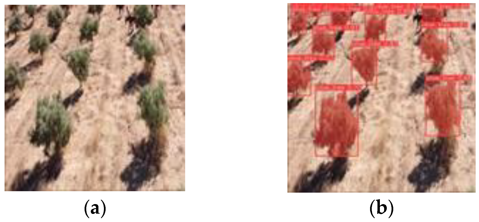
In addressing these challenges, the project utilized three publicly available datasets obtained from Roboflow [50,51,52], all related to olive tree analysis. All datasets feature images with a resolution of 640 × 640 pixels and are singularly focused on a unified class—“olive trees”. As shown in

Table 1. Datasets.

Dataset	Train Split	Valid Split	Test Split	Total	b/Image	Instances
DATASET1	622	137	127	886	78.9	52,837
DATASET2	155	50	38	243	82.3	14,202
DATASET3	67	19	9	95	8.2	681

, the first dataset, “DATASET1” [50], an indicative portion of which is depicted in Figure 4, is the largest among the three and comprises 622 training images, 137 validation images, and 127 test images. On average, each image contains 78.9 boxes (b/image), totaling 52,837 instances of olive trees. The second dataset “DATASET2” [51], sampled in Figure 5, consists of 155 training images, 50 validation images, and 38 test images. The average number of boxes per image is 82.3, contributing to a total of 14,202 instances of olive trees. The third dataset. “DATASET3” [52], indicated in Figure 6, focused on segmentation, is comparatively smaller. It includes 67 training images, 19 validation images, and 9 test images, with an average of 8.2 masks per image. In total, this dataset comprises 681 instances of olive trees. This dataset selection strategy ensures relevance to the objectives, providing diverse and sufficiently challenging data for the development and evaluation of the olive tree segmentation model.

Ground sampling distance (GSD) is a crucial concept in photogrammetry, where it determines the clarity and detail of aerial images. It refers to the distance between the centers of two consecutive pixels as measured on the ground. This metric helps determine an image’s spatial resolution; a smaller GSD means higher resolution, allowing for more detailed images, whereas a larger GSD results in lower resolution and less detail visible in the image. The GSD is calculated based on the following equation (x):

$$GSD={\displaystyle \frac{H\times SW}{F\times ImW}}$$

where $H$ is the flight height, $SW$ is the width of the camera sensor, $F$ is the focal length of the camera, and $ImW$ is the width of the captured image in pixels.

From the openly available datasets we examined in this paper, only DATASET3 was accompanied by the appropriate metadata containing valuable information for determining the flight height and calculating the GSD. Moreover, the images in DATASET1 and -2 do not adhere to central projection, and the wide capturing angles increase the perspective distortion. Therefore, calculating the GSD accurately is infeasible.

Images in the DATASET3 were captured using a DJI FC6310R drone camera, and each image includes raw metadata, such as latitude, longitude, GPS altitude, focal length, and width of camera sensor. The specific drone captured images with an image width of 5472 and image height of 3648. It is noted that this dataset comprises images from two different areas, both located in Morocco. Moreover, it is observed that a subset of the images retain the initial resolution at which the drone camera captured the images, while another set is cropped, likely due to some preprocessing performed by the creators of the dataset. However, for both subsets, the original image resolution is used to calculate the GSD values, and they are listed in

Table 2. GSD values for full-resolution and cropped images in DATASET3.

	Sw	FR	H	ImW	ImH	GSD
Full-resolution images	24	8.8	77	5472	3648	3.64
Crop images	24	8.8	111	5472	3648	5.53

.

4.2. Evaluation Metrics

The performance of the segmentation model was evaluated using several standard metrics, as follows: precision, recall, mean average precision at an intersection over union (IoU) threshold of 50 (mAP50), and mean average precision across IoU thresholds ranging from 50% to 95% (mAP50-95). Precision measures the proportion of correctly identified pixels classified as belonging to the object of interest. Recall indicates the proportion of all actual object pixels that were correctly identified by the model. mAP50 and mAP50-95 provide a more comprehensive evaluation by considering the trade-off between precision and recall at different IoU thresholds. IoU measures the overlap between the predicted and ground truth segmentation masks, with higher values indicating better agreement. A higher mAP value signifies the model’s ability to accurately segment objects across a range of overlap criteria.

4.3. System Specifications

Both training/fine-tuning and inference were conducted on a GPU NVIDIA RTX A4500 64GB. The framework of choice was Pytorch, and it was used for all deployments.

4.4. Experiments on RepViT-SAM/EdgeSAM for Segmentation

The suggested pipeline combines YOLOv8n-det, as the olive tree detector, with RepViT-SAM for olive tree segmentation. However, since the pretrained YOLOv8n-det model does not recognize the class “olive trees” or even “trees”, it needs fine-tuning. The YOLOv8n-det model was fine-tuned on the merged DATASET1 and DATASET2 (Merged), comprising 777 training images for 100 epochs, with early stopping patience set to 10 epochs and default hyper-parameters. Training concluded after 42 epochs, achieving a mean average precision at 50 IoU (mAP50) of 0.93285, as depicted in Figure 7. Inference involved using the fine-tuned YOLOv8n-det on the test split of DATASET1 to detect bounding boxes, which were then passed to RepViT-SAM/EdgeSAM for final segmentation (Figure 8). The total inference time for both models on the GPU was 4.3 ms for YOLOv8n-det and 64.31 ms for RepViT-SAM or 57.2 ms for EdgeSAM, resulting in a total inference time exceeding 60 ms. While this approach simplifies fine-tuning using available data, it relies on two resource-intensive models, impacting inference time and resource requirements.

4.5. Experiments on YOLOv8-Seg for Segmentation

Similarly to the first approach, YOLOv8n-seg requires fine-tuning since the pretrained model does not recognize the class “olive trees” or “trees”. To overcome the absence of a dedicated segmentation dataset, a custom segmentation dataset was created using DATASET1 and RepViT-SAM. An extensive evaluation was conducted by an expert who visually evaluated the results accepting only the correct masks.

In this procedure, RepViT-SAM was applied to all images in the detection dataset, utilizing corresponding bounding boxes for segmentation. The resulting segmentation masks, initially in binary form, underwent a transformation into polygons compatible with YOLO. A custom script was employed to execute these transformations and store the outcomes as .txt files for each image. To enhance the performance and increase generalization capabilities, we integrated the DATASET3 into the custom annotated segmentation dataset.

Before merging the two datasets, a straightforward data augmentation technique was employed, involving horizontal flips and random rotations, as depicted in Figure 9. This augmentation was specifically applied to the third dataset, generating augmented images for each original image. The considerable imbalance between the two datasets influenced the decision to apply data augmentation solely to one dataset. To achieve a more balanced outcome while maintaining enough images, we up-sampled the smaller dataset to approximately 150 images and retain only 150 images from the larger dataset. The final merged dataset (Merged_seg) comprised 323 training images, with an average number of masks per image set at 39.7. This strategy aimed to address the inherent dataset imbalance and enhance the model’s ability to generalize across diverse scenarios, contributing to the overall robustness of the segmentation model.

YOLOv8n-seg was fine-tuned on this merged custom dataset, involving 323 training images with an average number of 39.7 masks per image for 100 epochs, with early stoppage at 10 epochs and default hyper-parameters. The training stopped after 64 epochs achieving 0.761 mAP50, as illustrated in Figure 10. The fine-tuned YOLOv8n-seg model was used directly for predicting segmentations on input images. The inference time for YOLOv8n-seg was 4.3 ms. Consequently, during drone-based inference only the YOLOv8n-seg model was utilized, ensuring faster inference times, and the results of drone-based inference using YOLOv8-seg are shown in Figure 11.

Finally, an optimal threshold value of 0.35 was established through experimentation to achieve the most effective results for this specific application. While the default confidence threshold within YOLOv8n was 0.25, a systematic evaluation was conducted using five distinct thresholds. A visual quantitative analysis was conducted to choose this threshold, since it offered a balance between duplicate masks and missed masks. This evaluation process revealed that a threshold of 0.35 yielded superior performance for the olive tree segmentation task.

4.6. Methods Comparison and Discussion

For each lightweight model of the two proposed pipelines for olive tree segmentation on drone images, an evaluation was conducted both on the merged dataset, consisting of DATASET1 and DATASET2, as well as on each individual dataset, to better understand how the datasets affect the models’ performance and to achieve more robust evaluation results. Overall YOLOv8-seg model achieved slightly better results (mAP50 = 0.825,

Table 3. YOLOv8-seg evaluation results. (Bold indicates the best values).

Method	Precision (M)	Recall (M)	mAP50 (M)	mAP50-95 (M)	Inf. Time
DATASET1	0.898	0.868	0.919	0.626	4.6
DATASET2	0.941	0.943	0.971	0.721	10.7
DATASET3	0.955	0.763	0.863	0.666	3.2
Merged	0.842	0.774	0.825	0.667	3.5

) compared to the two variants of the SAM-based pipeline (mAP = 0.822 for RepViT-SAM,

Table 4. RepViT-SAM evaluation results. (Bold indicates the best values).

Method	Precision (M)	Recall (M)	mAP50 (M)	mAP50-95 (M)	Inf. Time
DATASET1	0.925	0.847	0.817	0.646	41.3
DATASET2	0.919	0.886	0.833	0.718	43.4
DATASET3	0.927	0.874	0.845	0.682	25.1
Merged	0.923	0.862	0.822	0.679	41.9

; mAP = 0.796 for EdgeSAM,

Table 5. EdgeSAM evaluation results. (Bold indicates the best values).

Method	Precision (M)	Recall (M)	mAP50 (M)	mAP50-95 (M)	Inf. Time
DATASET1	0.917	0.808	0.794	0.586	35.5
DATASET2	0.867	0.921	0.811	0.663	43.5
DATASET3	0.875	0.886	0.821	0.642	25.3
Merged	0.891	0.962	0.796	0.63	42.6

). Since YOLOv8-seg relies only on one model, there is no risk of compound failure, as there is the SAM-based pipeline where two models are required and any possible failure in the automated labeling process may affect the final result. In terms of inference time, again YOLOv8-seg achieved a noticeably better time (3.5 ms, Table 3) compared to the other two models (39.92 ms for RepViT-SAM, Table 4; 40.61 ms for EdgeSAM, Table 5). The simplicity of the YOLOv8-seg pipeline, where only this model was used for inference, caused this difference in inference times compared to the SAM-based pipeline, where two models are needed for inference, while also having a more complex model for segmentation than YOLOv8-seg.

The results from the evaluation of the three models on each individual dataset, as shown in Table 3, Table 4 and Table 5, indicate that no significant bias of any dataset affected the results in such a way that is worth mentioning, since the evaluation metrics were very balanced for the different datasets on all models. As for the inference time, a slight increase was observed for DATASET2 compared to DATASET1, which is normal since the average number of bounding boxes per image was larger for DATASET2, as shown in Table 1. The inference time for DATASET3 was, as expected, lower than those of the other datasets, since it had a much smaller average number of bounding boxes per image. These observations imply that the number of instances per image plays a pivot role in the inference time of the segmentation process. So, assuming a smart agriculture task of interest desired to be executed directly on an edge device, such as a UAV, the inference time is a crucial factor for the delivery of such a service. Moreover, as the computing capabilities in this case are limited, inference time should be kept at most in the order of tens of milliseconds. In addition to the hardware equipment and based on the results in Table 3, Table 4 and Table 5, capturing images at lower heights, so at a lower UAV flight height, may lead to better inference times.

The flight height, which is the distance of the camera sensor above the canopy, can be considered, since the camera sensor resides at the bottom part of the UAV. Then, the appropriate height range for having a single instance per image depends on multiple parameters, which relate the olive grove design, age or size of the trees, and the camera sensor per se. Several techniques can be considered for the olive grove design and tree spacing. According to production techniques suggested by the International Olive Council [49], orchard designs for olive trees include squares, offset squares, rectangles, and quincunxes. For precision farming, the square and offset square designs would be the most prominent choices, since they both provide good access to sunlight, as well as good coverage by precision farming tools due to fewer shadows and obstructions. Other designs or super-intensive orchards would be less appropriate for precision farming, as in these cases the trees develop in a hedgerow and complicate detection processes. So, for square or offset-square designs, planting distances of 6 m × 6 m and 7 m × 7 m are a sound yardstick for many Mediterranean olive-growing conditions [49].

In addition, the age of the olive, variety, and general management practice impact on the area covered by the canopy and the tree height. Indicatively, the height of mature trees of the koroneiki variety, which is widely cultivated for olive oil production, can reach 6–8 m when it is traditionally cultivated. However, it is usually controlled through pruning to stay at lower heights, between 4 m and 6 m, in order to be better managed and facilitate mechanical harvesting.

Furthermore, the camera characteristics affect the ground resolution, achieved per flight height. We considered the GSD for investigating appropriate flight heights. Indicatively, Parrot Sequoia is a widely used camera connected to UAVs for precision agriculture tasks. Its RGB sensor has an image width of 4608 px, a focal length equal to 4.88 mm, and the sensor width equals 6.09 mm. So, for a UAV equipped with this sensor, the recommended flight would be between 6.5 m and 7.4 m, in order to achieve, at most, one complete tree instance per image and, thus, optimize the inference time.

The SAM-based approach simplifies the fine-tuning process by directly fine-tuning the YOLOv8-det on the available limited detection data. However, in this approach, the inference process relies on two resource-intensive models, YOLOv8-det for detection and RepViT-SAM/EdgeSAM for segmentation, impacting the inference time and resource requirements. In essence, the YOLOv8-seg approach offers a simpler inference pipeline but requires creating a custom segmentation dataset through a more complex process that leverages RepViT-SAM/EdgeSAM and limited open-source olive tree datasets, since in order to fine-tune the YOLOv8-seg model, a segmentation dataset is required. Consequently, during the inference process of the second approach, only the YOLOv8n-seg model was utilized, ensuring potentially faster inference times and fewer resource requirements.

The confusion matrices in

Table 6. Confusion matrices.

	YOLO				RepViT-SAM				EdgeSAM
	D/S1	D/S2	D/S3	Merged	D/S1	D/S2	D/S3	Merged	D/S1	D/S2	D/S3	Merged
TP	6825	2160	58	2659	6660	2030	66	2962	6353	2110	67	3305
FP	775	135	3	499	540	179	5	247	575	324	10	404
FN	1038	131	18	777	1203	261	10	474	1510	181	9	131

present the performance of the three models—YOLOv8-seg, RepViT-SAM, and EdgeSAM—across various datasets, highlighting the nuanced differences in their segmentation capabilities. YOLOv8-seg consistently demonstrates superior performance, reflected by higher true positive (TP) counts and lower false positive (FP) and false negative (FN) counts across all datasets. For example, on DATASET1, YOLOv8-seg achieved 6825 TPs, 775 FPs, and 1038 FNs, indicating a high detection rate with minimal errors. This trend suggests that YOLOv8-seg is particularly adept at accurately identifying olive trees, thereby reducing both false alarms and missed detections.

In contrast, the SAM-based models, RepViT-SAM and EdgeSAM, exhibited higher error rates. RepViT-SAM, while achieving 6660 TPs on DATASET1, also incurred 540 FPs and 1203 FNs. Similarly, EdgeSAM recorded 6353 TPs but with 575 FPs and a significant 1510 FNs. These results indicate that the SAM-based models, despite their potential for fine-tuning ease, struggle with higher incidences of both false positives and negatives. This discrepancy can be attributed to the more complex inference pipelines of the SAM-based models, which involve multiple stages of detection and segmentation, potentially compounding errors at each step.

The variability in performance across different datasets also highlights the importance of dataset characteristics in the model evaluation. The consistent results of YOLOv8-seg across datasets suggest robust generalization capabilities, whereas the higher variance in the SAM-based models’ performances points to a sensitivity to specific dataset features. This sensitivity may necessitate more extensive fine-tuning and optimization for different agricultural contexts. Overall, the comparative analysis underscores the practical advantages of YOLOv8-seg in terms of both accuracy and efficiency, despite its more demanding initial setup. The SAM-based models, while promising, require further refinement to achieve comparable robustness and reliability in diverse real-world scenarios.

Since the YOLOv8-seg model outperformed the other two models, it was chosen for k-fold cross-validation to examine the stability of the model and the uniformity of the dataset. The k-fold cross-validation analysis, conducted over five iterations, assessed the performance of our model using metrics including precision, recall, mAP50, and mAP50-95. This method ensured a comprehensive evaluation, examining how consistently the model performed across different subsets of the data. As shown in

Table 7. K-fold validation results with YOLOv8-seg.

Fold	Precision (M)	Recall (M)	mAP50 (M)	mAP50-95 (M)
1	0.883	0.834	0.878	0.606
2	0.905	0.775	0.806	0.587
3	0.909	0.863	0.892	0.628
4	0.898	0.916	0.961	0.725
5	0.923	0.902	0.934	0.688
Average	0.903	0.858	0.894	0.647
STD	0.014	0.056	0.059	0.058

, precision varied slightly across the folds, with an average of 0.903, suggesting a high level of accuracy in the model’s predictions, with fewer false positives. Recall was generally lower than precision, with an average of 0.858, indicating the model’s ability to find all relevant instances is slightly less consistent than its precision. The mAP50 scores were strong, with an average of 0.8942, which highlights the model’s effectiveness at detecting objects when considering a 50% IoU threshold. mAP50-95, which averages the mAP over the IoU thresholds from 50% to 95%, had an overall lower performance compared to mAP50, averaging 0.6468. This expected decline across higher IoU thresholds indicates the model’s challenges in achieving precise localization under stricter conditions.

The bar chart depicted in Figure 12 reflects these dynamics, illustrating the variability across folds and metrics. The precision remained relatively stable, whereas recall showed more fluctuation, suggesting that some folds may contain particularly challenging examples. The mAP metrics demonstrate that while the model performs robustly at a basic IoU threshold (50%), its performance became more variable as the criteria tightened (up to 95% IoU). Also, the calculated standard deviations, shown in Table 7, reveal insights into the model’s performance consistency across different data scenarios. While precision was notably stable, the variability in recall and mAP metrics highlights potential challenges in model generalization, especially under more stringent evaluation criteria. Overall, the model demonstrated a robust performance with high precision and good overall mAP scores, indicating reliable detection capabilities. However, the variability in recall and mAP50-95 suggests potential areas for improvement, especially in enhancing the model’s ability to consistently localize objects more precisely across all data subsets.

Overall, this work tackled the data scarcity problem for the task of olive tree segmentation using drone images by proposing two distinct methodologies that do not rely on segmentation datasets but can leverage limited existing detection datasets by combining lightweight segmentation models. In the SAM-based approach, the YOLOv8-det was fine-tuned on those publicly available detection datasets and then used for inference along with RepViT-SAM/EdgeSAM for the final segmentation. On the YOLO-based approach, YOLOv8-seg is fine-tuned on a custom segmentation dataset created using some simple augmentation techniques and RepViT-SAM/EdgeSAM custom segmentation of the existing detection datasets. The YOLO-based approach achieved better results both in the metrics scores and in inference times.

5. Conclusions

The paper successfully highlights the significant potential and challenges of using drone imagery for olive tree segmentation, an innovative approach aimed at enhancing precision agriculture practices in olive cultivation. The paper pioneers the development of a custom annotated olive tree segmentation dataset and the application of lightweight variants of deep learning models like YOLOv8 and SAM to address the challenges of data scarcity and computational limitations on drones. These proposed pipelines bypass the labor-intensive process of manual segmentation annotation by utilizing publicly available detection datasets but also consider the models’ appropriateness for real-time inference with drones. Specifically, the YOLOv8-seg pipeline achieves higher scores with better inference time but requires a complex fine-tuning process due to a lack of publicly available segmentation datasets for olive trees. On the other hand, the SAM-based pipelines offer a much simpler fine-tuning process that can work with existing detection datasets of olive trees but comes with the cost of a much more complex inference architecture relying on two models resulting in lower metrics and higher inference time. The findings from the K-fold validation underscore areas for potential model refinement and underscore the importance of considering a larger dataset with greater diversity in training and validation processes to enhance overall model robustness.

These results provide a significant contribution to enabling real-time olive tree segmentation directly via UAVs, which constitute edge devices in the meta-OS context. As future work, the authors of this paper aim to create a robust and diverse public dataset for olive tree segmentation to address identified inconsistencies, while also testing the proposed methodologies in resource-constrained environments such as drones. In order to achieve this, the authors aim to validate the outcomes of this work within the Smart Farming pilot of the NEMO project [53], which aims to pilot meta-OS capabilities for autonomous aerial spraying. The pilot activities will involve deployment of the methods investigated with a UAV over an organic olive grove in Greece in order to identify the olive trees, triggering aerial precision spraying.