Multi-Unmanned Aerial Vehicles Cooperative Trajectory Optimization in the Approaching Stage Based on the Attitude Correction Algorithm

Abstract

This study investigated the problem of multi-UAVs cooperative trajectory optimization for remote maritime targets in the approach phase. First, based on the precise location information of the cooperative target, a real-time algorithm for correcting UAV attitude angles is proposed to reduce the impact of UAV attitude angle errors and observation system errors on target positioning accuracy. Then, the attitude correction algorithm is integrated into the interacting multiple model-cubature information filter (IMM-CIF) algorithm to achieve the fusion of multi-UAVs observation information. Furthermore, an improved receding horizon optimization (RHO) method is employed to plan the cooperative observation trajectories for UAVs in real time at the target approaching stage. Finally, numerical simulations are conducted to examine the proposed attitude correction and trajectory optimization algorithm, verifying the effectiveness of the proposed method and enhancing the tracking accuracy of the remote target.

1. Introduction

With the continuous development of future combat and weapon performance, the range of target engagement is increasing, which requires the high accuracy and stability of target information. Therefore, the effective tracking of remote targets has become an urgent task. Compared with a single unmanned aerial vehicle (UAV), which has a limited field of view, poor fault tolerance, and limited detection capabilities, multi-UAVs cooperative observation can provide multi-angle and multi-level reconnaissance of targets, thereby obtaining more target information and improving detection accuracy [1,2]. In addition, cooperative observation by multi-UAVs has significant advantages in fault tolerance and flexibility, thus attracting more attention and becoming one of the main research directions in target tracking.

UAV detection accuracy mainly involves two factors: the attitude angle accuracy of the navigation [3] and the observation accuracy of the sensor [4,5]. Since existing navigation systems lack a mature system for directly measuring the attitude angle of UAVs, the observability of the attitude angle is poor, and as time goes on, the cumulative errors in attitude angles will increase. In addition, the existence of the UAV attitude angle error is coupled with the sensor system error, resulting in time-varying sensor system errors, which cannot be ignored for remote maritime targets. Hence, enhancing the precision of remote target tracking with multi-UAVs encompasses two primary challenges. The first lies in minimizing the impact of the UAV attitude angle error and sensor system error on target localization accuracy. The second involves optimizing the trajectory planning for UAVs to reduce the impact of sensors’ random errors on the estimated state of the target. Scholars have conducted extensive research on these two issues.

In the field of system error reduction in attitude angle and observation, there are generally two types of error estimation models. The first type is the full-state augmentation model, which estimates the sensor system error and attitude angle system error as a state vector. Cui et al. [6] proposed an improved exact algorithm (EX) and then extended the improved EX algorithm to effectively estimate attitude angle errors and sensor system errors, addressing the system error registration problem of a mobile radar. However, this algorithm is greatly influenced by measurement points and lacks stability. In [7], the maximum likelihood error registration algorithm based on a fixed platform is extended to a mobile platform, and the problem of attitude angle system error in the mobile platform is further considered, which realizes the effective estimation of sensor system errors, attitude angle system errors, and target states. However, this algorithm is an offline estimation method and cannot solve the problem of real-time sensor system error registration. The Cubature Kalman Filter (CKF) is used to realize the online estimation of the attitude system error and the sensor observation system error in the literature [8].

The second model is the decoupled full-dimensional model, which equivalently considers the attitude angle system error as the sensor system error. Xiong Wei et al. [9] established a state equation and measurement equation for the system error based on the equivalent measurement error caused by the attitude angle error of sensors, and they used the Unscented Kalman Filter (UKF) to estimate the system error of attitude angle and sensor measurement angle. In addition, the position information of the cooperative target was used to equivalently convert the attitude angle error of the motion platform into a part of the sensor observation system error, establishing a decoupling model of sensor system errors to achieve a real-time estimation of attitude angle system error and sensor system error in [10]. Wang et al. [11] employed a linearization approach to derive an equivalent measurement error resulting from the attitude angle system error, and they treated the system error of the azimuth and pitch angle as a single variable to construct the state and measurement equations. Subsequently, they utilized the Kalman Filter (KF) for estimating the system error. Based on the work of Wang et al., the square root UKF was used to estimate the system error variables, and the result showed that linearization is not the main reason for the poor estimation of the attitude angle system error, but the observability of the attitude angle is the main factor [12].

In the field of multi-UAVs cooperative trajectory optimization, the state estimation of targets can enhance the accuracy of cooperative observation and help UAVs to plan flight trajectory effectively. Additionally, cooperative control can optimize the observational configuration of the UAVs and obtain a higher quality of observation information. Cooperative control and target state estimation are two closely related processes. Therefore, trajectory optimization involves two main issues: target state estimation and multi-UAV cooperative control. In the context of state estimation for maneuvering target tracking, conventional techniques such as KF, Particle Filtering (PF), and CKF have difficulty in handling the coupling relationship between different pieces observation information. However, information filtering (IF) can obtain updated fusion estimates through simple addition operations, and its simple calculation and easy scalability make IF very suitable for multi-sensor fusion state estimation [13]. In addition, the Interacting Multiple Model (IMM) filtering algorithm has been proven to be one of the most cost-effective multi-model algorithms, and it is widely used in maneuvering target tracking. Therefore, the IF algorithm is embedded into the improved IMM to achieve the fusion estimation of multi-UAVs for maneuvering targets [14].

The effective trajectory optimization of multi-UAVs is a crucial part of cooperative detection. There are usually two methods for the trajectory optimization of multi-UAVs collaborative target tracking. The first method is the potential field method based on the optimal observation configuration. Frew et al. [15,16] used the Lyapunov guidance vector field (LGVF) to control multiple UAVs to maintain the distance tracking of stationary and moving targets. Reference [17] solved the three-dimensional cooperative trajectory optimization problem of multiple UAVs based on the LGVF method and proposed an improved perturbation fluid dynamics system method to achieve obstacle avoidance for UAVs. Reference [18] proposed an improved LGVF method to achieve the cooperative tracking of multiple UAVs to the target, and this guidance method can accelerate the convergence speed of the desired phase and improve the target state estimation compared to the LGVF. In addition, reference [19] proposed a strategy using vector fields to achieve the remote tracking of the target by UAV swarms. Zhao et al. [20] proposed a multi-sensor cooperative control strategy based on the artificial potential field method to achieve an autonomous optimized configuration of only range sensors in two-dimensional and three-dimensional spaces. Song et al. [21] proposed a differential geometric guidance method to achieve the standoff tracking of the moving target. Yao et al. [22] proposed a hybrid approach based on the LGVF and improved interference fluid dynamic system to address the tracking and obstacle avoidance problems of multiple UAVs towards targets. Kokolakis et al. [23] proposed a guidance law to achieve robust standoff target tracking. Reference [24] studied a heading rate control law based on the LGVF under unknown wind speed conditions, aiming to achieve cooperative standoff tracking using multiple UAVs while considering constraints on control inputs. Reference [25] proposed a fusion algorithm combining MPC with the standoff algorithm to address the real-time obstacle avoidance shortcomings of the standoff algorithm. Lin et al. [26] proposed an improved guidance law based on the coordinated turning equation to achieve target tracking and proved its asymptotic stability. Reference [27] proposed a target tracking guidance method constrained by the terminal line-of-sight (LOS) angle aimed at directing the defensive unmanned surface vehicle to follow a moving target in a specified direction. However, determining the optimal sensor configuration for multi-sensor optimal observation during the approach phase remains challenging and limits the applicability of potential field-based methods. Moreover, it is difficult to determine the optimal configuration for a multi-sensor system in the approaching-target phase, making it challenging to apply the potential field-based method to optimize the optimal observation trajectory in the approaching phase.

The second approach is a numerical method, which transforms the trajectory optimization problem into a parameter optimization problem and solves it using optimization algorithms. Reference [28] proposed a customized interior-point method for planning multi-UAV trajectories, and the simulation results demonstrated that the algorithm significantly reduces the solution time. Chai et al. [29] introduced a two-step gradient-based algorithm to address the spacecraft trajectory optimization problem, with simulations showing that the proposed method offers effective and computationally efficient solutions. Zhang et al. [30] employed a sequential convex optimization algorithm to solve nonlinear optimal control for UAV trajectory planning. Reference [31] presents a convex optimization algorithm to solve multi-UAV cooperative trajectory optimization problems, with numerical simulations verifying the effectiveness of the algorithm. Reference [32] presents a novel hybrid Particle Swarm Optimization algorithm to address the multi-UAVs path planning problem in the presence of numerous obstacles. However, the use of the interior point method often neglects performance constraints of sensor platforms and tends to fall into local optima. Additionally, convex optimization methods can yield more precise solutions, and their design is notably complex [33]. Reference [34] minimized the trace of the FIM using the RHO to obtain optimized trajectories for multi-UAVs. References [35,36] achieved optimal cooperative target tracking among multiple UAVs based on the RHO. Zhang et al. [37] employed the RHO algorithm to optimize trajectories for cooperative multi-UAVs detection using the trace of the FIM as an evaluation metric, but these methods failed to consider the impact of the UAV attitude angle error on the target trajectory optimization. Beck et al. [38] proposed a novel waypoint-model predictive control method for online task re-planning, characterized by low computational complexity and high flexibility. The idea of the RHO method is derived from the principles of predictive control, utilizing optimization across several steps within the rolling horizon to replace global optimization, which has certain advantages in dealing with uncertainty issues and is particularly suitable for the online optimization of multi-UAVs cooperative trajectory.

However, the existing target state estimation algorithms of multi-UAVs mostly focus on reducing the random errors of UAVs, without considering the impact of UAV attitude angle errors and system errors on target state estimation, and further considering their impact on multi-UAVs trajectory optimization. Consequently, in the process of multi-UAVs trajectory optimization, it is necessary to integrate the design of algorithms for reducing UAV attitude angle errors and observation errors to improve the accuracy of target state estimation. Additionally, the error reduction algorithm for UAV attitude angles and observation system errors is mostly based on the parameter estimation and registration of attitude angle system errors with the invariant model. However, the error between the attitude angles output by the navigation device and the true attitude angles exhibits a step-like signal jump, indicating that the system error of the attitude angles is time-varying. In the case of time-varying attitude angle system errors, the target state estimated by the existing error registration algorithm will become seriously worse. Therefore, this paper proposes an attitude correction method based on the cooperative platform, which improves the accuracy of the cooperative detection of the remote maritime target by optimizing the observation trajectory of multi-UAVs.

The contribution of this paper mainly lies in three aspects:

(1)

From the perspective of improving target accuracy, the precise positioning of the cooperative platform is utilized to correct the attitude angle of the UAV in real time, so as to reduce the impact of UAV attitude angle error and observation error on positioning, and thus obtain a more accurate target position.

(2)

A multi-UAVs cooperative trajectory optimization model under constraints is established based on the cooperative platform, which is combined with the target position after attitude correction to solve the information fusion problem for multi-UAVs cooperative detection.

(3)

An integrated trajectory optimization method is proposed to reduce the attitude angle error and observation error of multi-UAVs by combining the cooperation platform position and the improved RHO method.

The structure of this paper is as follows. Section 2 models the problem of multi-UAVs cooperative target tracking. In Section 3, the precise position of the cooperative platform is used to correct the attitude angle of the UAVs in real time. The method of optimizing the cooperative observation trajectory of multi-UAVs using the improved RHO algorithm is presented in Section 4. The algorithm based on the cooperative platform integration for reducing the attitude angle error and observation error of UAVs is presented in Section 5. In Section 6, simulations are carried out to verify the effectiveness of the proposed algorithm. Finally, a conclusion is given.

2. Problem Statement

The scenario of multi-UAVs cooperative tracking in the approaching-target phase is shown in Figure 1. In Figure 1, OXY stands for the reference coordinate system. As shown in Figure 1, each UAV approaches the target and measures the position, speed, and other pieces of information of the target from different observation directions using its onboard sensor. Combined with the attitude angles of the UAV measured by the inertial measurement unit, a relatively accurate target state information is obtained through filtering and estimation. However, due to the shortcomings of a single UAV, such as few carrying equipment, weak perception ability, and poor robustness, it is usually unable to meet the needs of continuous and accurate target tracking. Thus, multi-UAVs cooperative tracking is highly effective in avoiding tracking blind zones and improving the tracking accuracy.

Due to the uncertainty of measurements and target motion, the key challenge in multi-UAVs cooperative tracking is to address the following two issues. (1) Develop an attitude correction algorithm to mitigate the impact of UAV attitude angle errors and system errors on the precision of target localization. (2) Plan observation trajectories for multi-UAVs during the approach phase to the target, and implement a multi-sensor fusion filtering algorithm to achieve a higher accuracy in multi-UAVs cooperative tracking.

2.1. UAV Motion Model

In multi-UAV cooperative control, mathematical models of UAVs with autopilots are commonly used, which are practical for engineering applications. Assume that each UAV has a low-order flight controller that controls the UAV’s speed and heading rate through control commands, thus controlling the UAV’s flight state. The two-dimensional UAV flight model is modeled as follows.

$$\left(\begin{array}{c}\dot{x}\\ \dot{y}\\ \dot{\psi }\\ \dot{v}\\ \dot{\omega }\end{array}\right)=f(\mathit{x},\mathit{u})=\left(\begin{array}{c}v\cos \psi \\ v\sin \psi \\ \omega \\ -{\displaystyle \frac{1}{{\tau }_v}}v+{\displaystyle \frac{1}{{\tau }_v}}{u}_v\\ -{\displaystyle \frac{1}{{\tau }_{\omega }}}\omega +{\displaystyle \frac{1}{{\tau }_{\omega }}}{u}_{\omega }\end{array}\right)$$

(1)

$\mathit{x}={[x,y,\psi ,v,\omega ]}^T$ represents the state of the UAV, including the position, heading angle, speed, and heading angular velocity of the UAV. ${\tau }_v$ and ${\tau }_{\omega }$ are the speed time delay constant and angular velocity time delay constant related to the UAV and its flight state. $\mathit{u}={[u_v,u_{\omega }]}^T$ is the control input for the UAV, representing the speed control command of the autopilot and the heading angular velocity control command, subject to the following constraints:

$$\left|u_v-v_0\right|\le v_{\max }$$

(2)

$$\left|u_{\omega }\right|\le {\omega }_{\max }$$

(3)

where $v_0$ represents the cruising speed of the UAV; $v_{\max }$ and ${\omega }_{\max }$ represent the maximum range of speed variation and the maximum angular velocity of the UAV, respectively.

In order to facilitate the model predictive control of the UAV, it is necessary to convert the continuous-time UAV model in Equation (1) into the following discrete-time model through Euler integration:

$${\mathit{x}}_{k+1}=f_d({\mathit{x}}_k,{\mathit{u}}_k)={\mathit{x}}_k+T_{s}f({\mathit{x}}_k,{\mathit{u}}_k)$$

(4)

where ${\mathit{x}}_k={[x_k,y_k,{\psi }_k,v_k,{\omega }_k]}^T$, ${\mathit{u}}_k={[u_{vk},u_{\omega k}]}^T$, $T_s$ represents the sampling time.

2.2. Target Maneuvering Model

System state estimation actually consists of two parts: system modeling and state estimation algorithms. Accurate system modeling is the cornerstone of effective system state estimation. In the target motion process, the target’s position, velocity, and acceleration are treated as variables. ${\mathit{x}}_{t,k}={[x_k,{\dot{x}}_k,{\ddot{x}}_k,y_k,{\dot{y}}_k,{\ddot{y}}_k]}^T$; the state of the target includes the horizontal position, velocity, and acceleration, as well as the vertical position, velocity, and acceleration. Therefore, the system equations can be represented in the following form [39]:

$${\mathit{x}}_{t,k}=\mathit{F}{\mathit{x}}_{t,k-1}+\mathit{G}{\mathit{w}}_{k-1}$$

(5)

where ${\mathit{x}}_{t,k}$ denotes the target state at time $k$, $\mathit{F}$ denotes the state transition matrix, $\mathit{G}$ denotes the transfer matrix of noise, ${\mathit{w}}_{k-1}$ denotes the zero-mean Gaussian process noise at time $k-1$, and the process noise covariance matrix is $Q_k$.

(1) When the target is moving at a constant speed, the model motion parameters of Equation (5) are

$$\mathit{F}=\left[\begin{array}{cccccc}1& T_s& 0& 0& 0& 0\\ 0& 1& 0& 0& 0& 0\\ 0& 0& 0& 0& 0& 0\\ 0& 0& 1& T_s& 0& 0\\ 0& 0& 0& 1& 0& 0\\ 0& 0& 0& 0& 0& 0\end{array}\right], \mathit{G}=\left[\begin{array}{cc}0.5{T_s}^2& 0\\ T_s& 0\\ 0& 0\\ 0& 0.5{T_s}^2\\ 0& T_s\\ 0& 0\end{array}\right]$$

(2) For a uniform acceleration of the target, the model motion parameters of Equation (5) are as follows:

$$\mathit{F}=\left[\begin{array}{cccccc}1& T_s& 0.5{T_s}^2& 0& 0& 0\\ 0& 1& T_s& 0& 0& 0\\ 0& 0& 1& 0& 0& 0\\ 0& 0& 0& 1& T_s& 0.5{T_s}^2\\ 0& 0& 0& 0& 1& T_s\\ 0& 0& 0& 0& 0& 1\end{array}\right], \mathit{G}=\left[\begin{array}{cc}{T_s}^3/6& 0\\ {T_s}^2/2& 0\\ T_s& 0\\ 0& {T_s}^3/6\\ 0& {T_s}^2/2\\ 0& T_s\end{array}\right]$$

(3) When the target is turning, the model motion parameters of Equation (5) are as follows, where $\Omega$ represents the model turning angular rate:

$$\begin{gathered} \mathit{F}=\left[\begin{array}{cccccc}1& {\displaystyle \frac{\sin \Omega T_s}{\Omega }}& {\displaystyle \frac{1-\cos \Omega T_s}{{\Omega }^2}}& 0& 0& 0\\ 0& \cos \Omega T_s& {\displaystyle \frac{\sin \Omega T_s}{\Omega }}& 0& 0& 0\\ 0& -\Omega \sin \Omega T_s& \cos \Omega T_s& 0& 0& 0\\ 0& 0& 0& 1& {\displaystyle \frac{\sin \Omega T_s}{\Omega }}& {\displaystyle \frac{1-\cos \Omega T_s}{{\Omega }^2}}\\ 0& 0& 0& 0& \cos \Omega T_s& {\displaystyle \frac{\sin \Omega T_s}{\Omega }}\\ 0& 0& 0& 0& -\Omega \sin \Omega T_s& \cos \Omega T_s\end{array}\right] \\ \mathit{G}=\left[\begin{array}{cc}{T_s}^3/6& 0\\ {T_s}^2/2& 0\\ T_s& 0\\ 0& {T_s}^3/6\\ 0& {T_s}^2/2\\ 0& T_s\end{array}\right] \end{gathered}$$

2.3. UAV Observation Model

The sensor carried by the UAV can measure the angle and distance of the target. The measurement z of the sensor can be modeled according to the position of the UAV ${(x,y)}^T$ and the target position ${(x_t,y_t)}^T$ as

$$\mathit{z}(k)=\left(\begin{array}{c}{r}_k\\ {\theta }_k\end{array}\right)=h({\mathit{x}}_k,{\mathit{x}}_{t,k})+{\mathit{v}}_k=\left(\begin{array}{c}\sqrt{{(x_{t,k}-x_k)}^2+{(y_{t,k}-y_k)}^2}\\ {\tan }^{-1}{\displaystyle \frac{y_{t,k}-y_k}{x_{t,k}-x_k}}\end{array}\right)+{\mathit{v}}_k$$

(6)

where $r_k$ and ${\theta }_k$ denote the distance and azimuth, respectively. $v_k$ denotes the zero-mean Gaussian observed noise; the observed noise covariance matrix is $R_k$, $R_k=\left[\begin{array}{cc}{\sigma }_r^2& 0\\ 0& {\sigma }_{\theta }^2\end{array}\right]$; ${\sigma }_r$ and ${\sigma }_{\theta }$ represent the standard deviations of the distance error and azimuth error of the UAV observing the target, respectively.

3. Target Tracking Based on the Attitude Correction Algorithm

The Inertial Measurement Unit (IMU) is the basic attitude measurement sensor. Due to the drift in IMU outputs, the accuracy of the UAV attitude estimation will deteriorate over time if only IMU outputs are used. Therefore, it is necessary to calibrate the attitude angles of the UAV. The cooperative platform can provide an accurate position, which can be used to correct the attitude of the UAV. In the target localization algorithm based on attitude calibration, the UAV is equipped with two sensors: one sensor observes the target, and the other sensor observes the cooperative platform. Firstly, the attitude angles of the UAV with smaller errors are calculated based on the accurate position information from the cooperative platform. Then, these attitude angles are used for target localization, resulting in more accurate target positions. The scenario of target localization based on attitude calibration is shown in Figure 2.

3.1. Target Localization Principle Using the UAV

In order to detail the target positioning process, it is necessary to introduce several coordinate systems.

The geographic coordinate system: the origin is fixed at a certain position on the ground, the $xOy$ plane is tangential to the surface, the x-axis points to the east, the y-axis points to the north, and the z-axis points to the zenith. It is denoted by subscript g.

The UAV stable coordinate system: the origin is fixed at the center of mass of the UAV, and the coordinate axes are parallel to those of the geographic coordinate system. It is denoted by subscript b.

The UAV body coordinate system: the origin is fixed at the center of mass of the UAV, the x-axis points to the direction of the UAV, the y-axis is perpendicular to the x-axis within the UAV’s cross-section, and the z-axis is perpendicular to the $xOy$ plane pointing above the UAV. It is denoted by subscript u.

Let the UAV attitude angles be $\mathsf{\vartheta }=(\psi ,\theta ,\varphi )$ (yaw, pitch, roll), and let the transformation matrix from the body coordinate system coordinates to the body geographic coordinate system coordinates be ${\mathit{M}}_{us}$.

$${\mathit{M}}_{us}(\mathsf{\vartheta })={\mathit{M}}_{\psi }(\psi ){\mathit{M}}_{\theta }(\theta ){\mathit{M}}_{\varphi }(\varphi )$$

(7)

where

$${\mathit{M}}_{\psi }(\psi )=\left(\begin{array}{ccc}\cos \psi & \sin \psi & 0\\ -\sin \psi & \cos \psi & 0\\ 0& 0& 1\end{array}\right)$$

(8)

$${\mathit{M}}_{\theta }(\theta )=\left(\begin{array}{ccc}1& 0& 0\\ 0& \cos \theta & \sin \theta \\ 0& -\sin \theta & \cos \theta \end{array}\right)$$

(9)

$${\mathit{M}}_{\psi }(\psi )=\left(\begin{array}{ccc}\cos \psi & \sin \psi & 0\\ -\sin \psi & \cos \psi & 0\\ 0& 0& 1\end{array}\right)$$

(10)

The position of the target in the geographic coordinate system is represented as follows:

$${\mathit{X}}_{t,g}={\mathit{X}}_{f,g}^{*}+{\mathit{M}}_{us}(\mathsf{\vartheta }){\mathit{X}}_{tob,u}$$

(11)

${\mathit{X}}_{f,g}^{*}$ represents the UAV’s position in the geographic coordinate system, and ${\mathit{X}}_{tob,u}$ represents the target’s position in the UAV body coordinate system, which can be expressed as follows:

$${\mathit{X}}_{tob,u}=\left(\begin{array}{c}{r}_t\cos {\beta }_t\cos {\epsilon }_t\\ r_t\sin {\beta }_t\cos {\epsilon }_t\\ r_t\sin {\epsilon }_t\end{array}\right)$$

(12)

where $r_t$, ${\beta }_t$, and ${\epsilon }_t$ represent the distance, azimuth angle, and elevation angle of the target observed by the UAV.

Formula (11) shows that the attitude angle $\mathsf{\vartheta }$ of the UAV affects the positioning accuracy of the target; therefore, a correction algorithm for reducing the attitude angle error is proposed in the next section.

3.2. Attitude Correction Algorithm Based on the Cooperative Platform

${\mathit{X}}_{c,g}$ is the position of the cooperative platform in the geographic coordinate system, and the measurement of the UAV on the cooperative platform is $\left(r_c,{\theta }_c,{\phi }_c\right)$, where $r_c$, ${\theta }_c$, and ${\phi }_c$ are the distance, azimuth angle, and elevation angle of the cooperative platform observed by the UAV. Therefore, the observed values of the cooperative platform in the UAV’s Cartesian coordinate system can be obtained:

$${\mathit{X}}_{cob,u}=\left(\begin{array}{c}{r}_c\cos {\theta }_c\cos {\phi }_c\\ r_c\sin {\theta }_c\cos {\phi }_c\\ r_c\sin {\phi }_c\end{array}\right)$$

(13)

In an ideal case, we should have

$${\mathit{X}}_{c,g}={\mathit{X}}_{f,g}^{*}+{\mathit{M}}_{us}(\mathsf{\vartheta }){\mathit{X}}_{cob,u}$$

(14)

However, due to the errors of attitude angles, observation, and UAV position, Equation (14) is not valid. Thus, it is necessary to solve $\mathsf{\vartheta }$ for minimizing $I(\mathsf{\vartheta })$.

$$I(\mathsf{\vartheta })=\left|{\mathit{X}}_{f,g}^{*}+{\mathit{M}}_{us}(\mathsf{\vartheta }){\mathit{X}}_{cob,u}-{\mathit{X}}_{c,g}\right|$$

(15)

The purpose of attitude correction is to find the optimal attitude ${\mathsf{\vartheta }}_{\min }$ to minimize $\mathit{I}(\mathsf{\vartheta })$, e.g., $\min \mathit{I}(\mathsf{\vartheta })=\mathit{I}({\mathsf{\vartheta }}_{\min })$, and ${\mathsf{\vartheta }}_{\min }$ can be obtained by solving Equation (15) by the gradient descent method. Using the correction value ${\mathsf{\vartheta }}_{\min }$ as the UAV’s attitude theoretically has a higher accuracy than the measurement value ${\mathsf{\vartheta }}^{*}$. Therefore, the more accurate target position is determined as follows:

$${\mathit{X}}_{t,g}={\mathit{X}}_{f,g}^{*}+{\mathit{M}}_{us}({\mathsf{\vartheta }}_{\min }){\mathit{X}}_{tob,u}$$

(16)

After obtaining precise observation measurements ${\mathit{X}}_{t,g}$ of the maritime target at multiple moments, the motion state of maritime targets is estimated through tracking filtering algorithms.

3.3. Target State Estimation Based on IMM-CIF Algorithm

The iterative process of the IMM-CIF algorithm includes four steps: state interaction, model matching filtering, model probability update, and interactive output. Assuming there are N motion models in the IMM algorithm, the model transition matrix can be represented as follows:

$$\mathbf{\Pi }=\left[\begin{array}{cccc}{p}_{11}& p_{12}& \cdots & p_{1N}\\ p_{21}& p_{22}& \cdots & p_{2N}\\ ⋮& ⋮& \ddots & ⋮\\ p_{N1}& p_{N2}& \cdots & p_{NN}\end{array}\right]$$

(17)

The steps of the IMM-CIF algorithm are as follows:

(1) State interaction. Based on the state variables, model probabilities, and covariance matrices of each model at time $k-1$, we obtain the initial state variables and covariance matrices of model $j$:

$$\{\begin{array}{l}{\mathit{X}}_{k-1|k-1}^{0j}={\displaystyle \sum _{i=1}^N{\mathit{X}}_{k-1|k-1}^i{\mathsf{\mu }}_{k-1}^{i/j}}\\ {\mathit{P}}_{k-1|k-1}^{0j}={\displaystyle \sum _{i=1}^N{\mathsf{\mu }}_{k-1|k-1}^{i/j}\left\{{\mathit{P}}_{k-1|k-1}^j+\left[{\widehat{\mathit{X}}}_{k-1|k-1}^i-{\widehat{\mathit{X}}}_{k-1|k-1}^{0j}\right]{\left[{\widehat{\mathit{X}}}_{k-1|k-1}^i-{\widehat{\mathit{X}}}_{k-1|k-1}^{0j}\right]}^T\right\}}\end{array}$$

(18)

where

$$\{\begin{array}{l}{\mathsf{\mu }}_{k-1}^{i/j}={\displaystyle \frac{p_{ij}{\mathsf{\mu }}_{k-1}^i}{C_j}}\\ C_j={\displaystyle \sum _{i=1}^N{p}_{ij}{\mathsf{\mu }}_{k-1}^i}\end{array}$$

(19)

${\mathsf{\mu }}_{k-1}^{i/j}$ is the conditional probability of model $i$ at time $k-1$, and ${\mathsf{\mu }}_{k-1}^i$ is the probability of model $i$ at time $k-1$.

(2) Model matching filtering (CIF). The initial states and covariance matrices of various models obtained from the input interaction steps, as well as the sensor observations, are used as inputs to the filter. By using the CIF filtering algorithm, the filtered state matrix ${\widehat{\mathit{X}}}_{k|k}^j$ and covariance matrix ${\mathit{P}}_{k|k}^j$ are obtained, and at the same time, the observation prediction value ${\widehat{\mathit{z}}}_{k|k-1}^j$ and residual ${\mathit{v}}_k^j$ can be obtained through the CIF filtering algorithm.

The likelihood function ${\Lambda }_k^j$ is expressed as follows:

$${\Lambda }_k^j={\displaystyle \frac{1}{\sqrt{2\pi {\mathit{V}}_k^j}}}\exp \left[-{\displaystyle \frac{1}{2}}\left({\mathit{z}}_k-{\widehat{\mathit{z}}}_{k|k-1}^j\right){\left({\mathit{V}}_k^j\right)}^{-1}{\left({\mathit{z}}_k-{\widehat{\mathit{z}}}_{k|k-1}^j\right)}^T\right]$$

(20)

(3) Model probability update. Update the model probability based on the likelihood function obtained from the previous step.

$${\mathsf{\mu }}_k^j={\displaystyle \frac{{\Lambda }_k^j{C}_j}{{\displaystyle \sum _{j=1}^N{\Lambda }_k^j{C}_j}}}$$

(21)

(4) Interactive output. Calculate the fused output based on the filtering result of step (2) and the model probability of step (3):

$$\{\begin{array}{l}{\widehat{\mathit{X}}}_{k|k}={\displaystyle \sum _{j=1}^N{\widehat{\mathit{X}}}_{k|k}^j{\mathsf{\mu }}_k^j}\\ P_{k|k}={\displaystyle \sum _{j=1}^N{\mathsf{\mu }}_k^j\left\{P_{k|k}^j+\left[{\widehat{\mathit{X}}}_{k|k}^j-{\widehat{\mathit{X}}}_{k|k}\right]{\left[{\widehat{\mathit{X}}}_{k|k}^j-{\widehat{\mathit{X}}}_{k|k}\right]}^T\right\}}\end{array}$$

(22)

In conclusion, the UAV target tracking algorithm based on attitude correction mainly consists of four steps:

(1)

The UAV simultaneously observes the cooperative platform and the maritime target through the sensors it carries, obtaining the observation matrix ${\mathit{X}}_{tob,u}$ for the maritime target according to Formula (12), as well as the observation matrix ${\mathit{X}}_{cob,u}$ for the cooperative platform according to Formula (13).

(2)

According to Equations (12)–(15), calculate the attitude angles ${\mathsf{\vartheta }}_{\min }$ based on the observation matrix ${\mathit{X}}_{cob,u}$ of the cooperation platform by the UAV and the known position ${\mathit{X}}_{c,g}$ of the cooperation platform.

(3)

Construct the transformation matrix ${\mathit{M}}_{us}({\mathsf{\vartheta }}_{\min })$ from the UAV body coordinate system to the geographic coordinate system using the correction attitude angle ${\mathsf{\vartheta }}_{\min }$, so that the precise position ${\mathit{X}}_{t,g}$ of the maritime target is obtained according to Equation (16).

(4)

Using the precise position ${\mathit{X}}_{t,g}$ of the maritime target at time $k$, the motion state of the target is estimated with a tracking filter algorithm.

4. Multi-UAVs Cooperative Observation and Trajectory Optimization

4.1. Trajectory Optimization Based on Minimizing the Cooperative Tracking Variance

According to the state equation and observation equation shown in Formulas (5) and (6), the prediction process and update process in single-UAV information filtering are as follows [37]:

(1) Prediction process:

$$\{\begin{array}{l}{\mathit{Y}}_{i,k|k-1}={\left({\mathit{F}}_k{\mathit{Y}}_{i,k-1|k-1}^{-1}{\mathit{F}}_k^T+{\mathit{G}}_k{\mathit{Q}}_k{\mathit{G}}_k^T\right)}^{-1}\\ {\widehat{\mathit{y}}}_{i,k|k-1}={\mathit{Y}}_{i,k|k-1}{\mathit{F}}_k{\widehat{\mathit{x}}}_{i,k-1|k-1}\\ {\widehat{\mathit{x}}}_{i,k|k-1}={\mathit{Y}}_{i,k|k-1}^{-1}{\widehat{\mathit{y}}}_{i,k|k-1}\end{array}$$

(23)

(2) Update process:

$$\{\begin{array}{l}{\mathit{Y}}_{i,k|k}={\mathit{Y}}_{i,k|k-1}+{\mathit{I}}_{i,k}\\ {\widehat{\mathit{y}}}_{i,k|k}={\widehat{\mathit{y}}}_{i,k|k-1}+{\mathit{i}}_{i,k}\\ {\mathit{I}}_{i,k}={\mathit{H}}_{i,k}^T{\mathit{R}}_{i,k}^{-1}{\mathit{H}}_{i,k}\\ {\mathit{i}}_{i,k}={\mathit{H}}_{i,k}^T{\mathit{R}}_{i,k}^{-1}\left[{\mathit{z}}_{i,k}+{\mathit{H}}_{i,k}{\widehat{\mathit{x}}}_{i,k|k-1}-h_i\left({\mathit{X}}_k\right)\right]\end{array}$$

(24)

In the above formula, $\widehat{\mathit{y}}(k|k-1)$ and $\mathit{Y}(k|k-1)$ are the predicted information state and predicted information matrix, respectively. $\mathit{Y}(k-1|k-1)$ is the information state matrix at time $k-1$, ${\mathit{H}}_i(k)$ is the Jacobian matrix of the measurement equation for the i-th UAV, ${\mathit{z}}_i(k)$ is the measurement information, and $\widehat{\mathit{x}}(k|k-1)$ is the predicted target state.

Based on the observation results of the single UAV mentioned above, the global information state and the Fisher information matrix for the multi-UAV observations are as follows:

$$\{\begin{array}{l}{\widehat{\mathit{y}}}_{k|k}={\widehat{\mathit{y}}}_{k|k-1}+{\displaystyle \sum _{i=1}^N{\mathit{i}}_{i,k}}\\ {\mathit{Y}}_{k|k}={\mathit{Y}}_{k|k-1}+{\displaystyle \sum _{i=1}^N{\mathit{I}}_{i,k}}\end{array}$$

(25)

The final estimated target state is ${\widehat{\mathit{x}}}_{k|k}={\mathit{Y}}_{k|k}^{-1}{\widehat{y}}_{k|k}$, and ${\widehat{\mathit{x}}}_{k|k}$ is used as input information to optimize the control output; $N$ is the number of UAVs.

Using the receding horizon optimization method to solve optimal control, at each discrete time, the system’s model is used to predict the state of a time period in the future. An optimization problem is established using the predicted future state of the system, and this optimization problem is solved online to obtain the optimal control sequence at this moment. At the next moment, the aforementioned process is repeated and optimized, and the performance function of UAV $i$ observing the target at time $k$ is as follows:

$${\mathit{J}}_{i,k}={\displaystyle \sum _{m=k}^{k+N_p}L({\mathit{x}}_{t,m},{\mathit{x}}_{i,m})}={\displaystyle \sum _{m=k}^{k+N_p}\left(-\left|{\displaystyle \sum _{i=1}^N{\mathit{Y}}_{i,m}}\right|\right)}$$

(26)

where $N_p$ is the predicted steps, ${\mathit{x}}_{i,m}$ and ${\mathit{x}}_{t,m}$ are the state variables of the $i$-th UAV and the target at time $m$, respectively. $L({\mathit{x}}_{t,m},{\mathit{x}}_{i,m})$ is a scalar function of the target state and UAV state at time $m$. Therefore, the cooperative target tracking problem of the multi-UAV is transformed into a nonlinear model optimization control problem that minimizes the objective function according to constraints, as shown in the mathematical model below:

$$\begin{array}{c}\underset{{\mathit{u}}_{i,k}^{*}}{\min }{\mathit{J}}_{i,k}\\ s.t.{\mathit{x}}_{i,k+1}-f_d({\mathit{x}}_{i,k},{\mathit{u}}_{i,k})=0\\ S_v({\mathit{u}}_{i,k})={\displaystyle \frac{\left|u_{i,vk}-v_0\right|-\Delta v_{\max }}{\Delta v_{\max }}}\le 0\\ S_{\omega }({\mathit{u}}_{i,k})={\displaystyle \frac{\left|u_{i,\omega k}\right|-{\omega }_{\max }}{{\omega }_{\max }}}\le 0\end{array}$$

(27)

In the above formula, ${\mathit{u}}_{i,k}$ represents the control input of the $i$th UAV at time k, $v_0$ is the cruising speed of the UAV, $v_{\max }$ is the maximum speed change, and ${\omega }_{\max }$ is the maximum turn rate.

The control flow chart of multi-UAV trajectory optimization based on the RHO method is given in Figure 3. According to Formulas (26) and (27), the minimum of the performance function ${\mathit{J}}_{i,k}$ at each moment can ensure that the optimal control sequence ${\mathit{u}}_{i,k}^{*}$ controls UAVs in the optimal observation position, and the accurate target state is obtained.

4.2. Optimization Solution Based on the RHO Method

To address the issue in Equation (27), a Lagrange multiplier vector $\mathsf{\lambda }$ and penalty factors ${\mu }_v,{\mu }_w$ are introduced. Consequently, the optimal control problem for the cooperative target tracking of the multi-UAV can be reduced to the problem of minimizing the following performance indicators.

$${\mathit{J}}_{i,k}={\displaystyle \sum _{m=k}^{k+N_p}L({\mathit{x}}_{t,m},{\mathit{x}}_{i,m})}+{\displaystyle \sum _{m=k}^{k+N_p-1}\left\{{\mathsf{\lambda }}_{m+1}^T(f({\mathit{x}}_{i,m},{\mathit{u}}_{i,m})-{\mathit{x}}_{i,m+1})+{\mathsf{\mu }}_v{l}_{v,m}{S}_v({\mathit{u}}_{i,m})+{\mathsf{\mu }}_{\omega }{l}_{\omega ,m}{S}_{\omega }({\mathit{u}}_{i,m})\right\}}, k=1,2,\dots ,N$$

(28)

$$l_{\ast ,m}=\{\begin{array}{l}0,\hspace{1em}{S}_{\ast ,m}\le 0\\ 1,\hspace{1em}{S}_{\ast ,m}>0\end{array}$$

The penalty function, denoted by $l_{\ast ,m}$, is zero when the control input satisfies the constraints, and it becomes sufficiently large when the constraints are violated.

Let Hamiltonian functions be

$$\begin{gathered} {\mathit{H}}_{i,m}=L({\mathit{x}}_{t,m},{\mathit{x}}_{i,m})+{\mathsf{\lambda }}_{m+1}^{T}f({\mathit{x}}_{i,m},{\mathit{u}}_{i,m})+{\mathsf{\mu }}_v{l}_{v,m}{S}_v({\mathit{u}}_{i,m})+{\mathsf{\mu }}_{\omega }{l}_{\omega ,m}{S}_{\omega }({\mathit{u}}_{i,m}), \\ m=k,k+1,\dots ,k+N_p-1 \end{gathered}$$

(29)

then

$$\begin{array}{ll}{\mathit{J}}_{i,k}& =L({\mathit{x}}_{t,k+N_p},{\mathit{x}}_{i,k+N_p})+{\displaystyle \sum _{m=k}^{k+N_p-1}\left\{{\mathit{H}}_{i,m}-{\mathsf{\lambda }}_{m+1}^T{\mathit{x}}_{i,m+1}\right\}}\\ & =L({\mathit{x}}_{t,k+N_p},{\mathit{x}}_{i,k+N_p})-{\mathsf{\lambda }}_{k+N_p}^T{\mathit{x}}_{i,k+N_p}+{\mathsf{\lambda }}_k^T{\mathit{x}}_{i,k}\\ & +{\displaystyle \sum _{m=k}^{k+N_p-1}\left\{{\mathit{H}}_{i,m}-{\mathsf{\lambda }}_m^T{\mathit{x}}_{i,m}\right\}}\end{array}$$

(30)

Taking the first-order variation of the above equation, we obtain

$$\begin{array}{l}\delta {\mathit{J}}_{i,k}={\left[{\displaystyle \frac{\partial L({\mathit{x}}_{t,k+N_p},x_{i,k+N_p})}{\partial {\mathit{x}}_{i,k+N_p}}}-{\mathsf{\lambda }}_{k+N_p}^T\right]}^T\delta {\mathit{x}}_{i,k+N_p}+{\mathsf{\lambda }}_k^T\delta {\mathit{x}}_{i,k}\\ \hspace{1em}\hspace{1em}+{\displaystyle \sum _{m=k}^{k+N_p-1}\left\{{\left[\frac{\partial H_{i,m}}{\partial {\mathit{x}}_{i,m}}-{\mathsf{\lambda }}_m^T\right]}^T\delta {\mathit{x}}_{i,m}+{\left[\frac{\partial H_{i,m}}{\partial {\mathit{u}}_{i,m}}\right]}^T\delta {\mathit{u}}_{i,m}\right\}}\end{array}$$

(31)

The necessary conditions for optimal control implementation are follows:

$${\mathsf{\lambda }}_{k+N_p}^T={\displaystyle \frac{\partial L({\mathit{x}}_{t,k+N_p},{\mathit{x}}_{i,k+N_p})}{\partial {\mathit{x}}_{i,k+N_p}}}$$

(32)

$${\mathsf{\lambda }}_m={\displaystyle \frac{\partial H_{i,m}}{\partial {\mathit{x}}_{i,m}}}$$

(33)

$${\displaystyle \frac{\partial {\mathit{H}}_{i,m}}{\partial {\mathit{x}}_{i,m}}}={\displaystyle \frac{\partial L({\mathit{x}}_{t,m},{\mathit{x}}_{i,m})}{\partial {\mathit{x}}_{i,m}}}+{\displaystyle \frac{\partial f^T({\mathit{x}}_{i,m},{\mathit{u}}_{i,m})}{\partial {\mathit{x}}_{i,m}}}{\mathsf{\lambda }}_{m+1}$$

(34)

Let $\mathit{Y}={\displaystyle \sum _{i=1}^n{\mathit{Y}}_{i,m}}$ and $L({\mathit{x}}_{t,m},{\mathit{x}}_{i,m})=-\left|\mathit{Y}\right|$. The relationship between derivatives and differentials indicates that

$$dL({\mathit{x}}_{t,m},{\mathit{x}}_{i,m})=\mathrm{trace}\left({{\displaystyle \frac{\partial L({\mathit{x}}_{t,m},{\mathit{x}}_{i,m})}{\partial \left|\mathit{Y}\right|}}}^{T}d\left|\mathit{Y}\right|\right)$$

(35)

According to $d\left(\left|\mathit{Y}\right|\right)=\left|\mathit{Y}\right|\mathrm{trace}\left({\mathit{Y}}^{-1}d\mathit{Y}\right)$,

$$\begin{array}{ll}dL({\mathit{x}}_{t,m},{\mathit{x}}_{i,m})& =\mathrm{trace}\left({{\displaystyle \frac{\partial L({\mathit{x}}_{t,m},{\mathit{x}}_{i,m})}{\partial \left|\mathit{Y}\right|}}}^{T}d\left|\mathit{Y}\right|\right)\\ & =-\mathrm{trace}\left(d\left|\mathit{Y}\right|\right)\\ & =-\mathrm{trace}\left(\left|\mathit{Y}\right|\mathrm{trace}\left({\mathit{Y}}^{-1}d\mathit{Y}\right)\right)\\ & =-\mathrm{trace}\left(\left|\mathit{Y}\right|\mathrm{trace}\left(2{\mathit{R}}_{i,m}^{-1}{\mathit{H}}_{x_{t,m}}{\mathit{Y}}^{-1}{\displaystyle \frac{\partial {\mathit{H}}_{{\mathit{x}}_{t,m}}}{\partial x_{i,m}}}d{\mathit{x}}_{i,m}\right)\right)\\ & =-\mathrm{trace}\left(\left|\mathit{Y}\right|\mathrm{trace}\left({\left({\left(2{\mathit{R}}_{i,m}^{-1}{\mathit{H}}_{x_{t,m}}{\mathit{Y}}^{-1}\right)}^T\right)}^T{\displaystyle \frac{\partial {\mathit{H}}_{x_{t,m}}}{\partial {\mathit{x}}_{i,m}}}d{\mathit{x}}_{i,m}\right)\right)\end{array}$$

(36)

Combined with $\mathrm{trace}({\mathit{A}}^T\mathit{B})={(\mathrm{vec}\mathit{A})}^T\mathrm{vec}(\mathit{B})$:

$$dL({\mathit{x}}_{t,m},{\mathit{x}}_{i,m})=-\left|\mathit{Y}\right|\mathrm{trace}\left({\left(\mathrm{vec}{\left(2{\mathit{R}}_{i,m}^{-1}{\mathit{H}}_{x_{t,m}}{\mathit{Y}}^{-1}\right)}^T\right)}^T\mathrm{vec}\left({\displaystyle \frac{\partial {\mathit{H}}_{{\mathit{x}}_{t,m}}}{\partial {\mathit{x}}_{i,m}}}d{\mathit{x}}_{i,m}\right)\right)$$

(37)

where $\mathrm{trace}(\cdot )$ denotes the trace of the matrix, and $\mathrm{vec}(\cdot )$ denotes the column vectorization of the matrix. The relationship between derivatives and differentials indicates that

$$dL({\mathit{x}}_{t,m},{\mathit{x}}_{i,m})=\mathrm{trace}\left({{\displaystyle \frac{\partial L({\mathit{x}}_{t,m},{\mathit{x}}_{i,m})}{\partial {\mathit{x}}_{i,m}}}}^{T}d{\mathit{x}}_{i,m}\right)$$

(38)

According to Equations (37) and (38), it is directly derived that

$$\begin{array}{ll}\frac{\partial L({\mathit{x}}_{t,m},{\mathit{x}}_{i,m})}{\partial {\mathit{x}}_{i,m}}& =-2\left|\mathit{Y}\right|{\left\{{\left[\mathrm{vec}\left({\mathit{R}}_{i,m}^{-1}{\mathit{H}}_{x_{t,m}}{\mathit{Y}}^{-1}\right)\right]}^T{\displaystyle \frac{\partial \mathrm{vec}{\mathit{H}}_{x_{t,m}}}{\partial {\mathit{x}}_{i,m}^T}}\right\}}^T\\ & =2L({\mathit{x}}_{t,m},{\mathit{x}}_{i,m}){\left\{{\left[\mathrm{vec}\left({\mathit{R}}_{i,m}^{-1}{\mathit{H}}_{x_{t,m}}{\left({\displaystyle \sum _{i=1}^n{\mathit{Y}}_{i,m}}\right)}^{-1}\right)\right]}^T{\displaystyle \frac{\partial \mathrm{vec}{\mathit{H}}_{x_{t,m}}}{\partial {\mathit{x}}_{i,m}^T}}\right\}}^T\end{array}$$

(39)

In Equation (39),

$${\mathit{H}}_{x_{t,l}}={\displaystyle \frac{\partial h_i({\mathit{x}}_k,{\mathit{x}}_{t,k})}{\partial {\mathit{x}}_{t,k}^T}}=\left[\begin{array}{cccc}{\displaystyle \frac{\Delta x_{i,k}}{r_{i,k}}}& 0& {\displaystyle \frac{\Delta y_{i,k}}{r_{i,k}}}& 0\\ -{\displaystyle \frac{\Delta y_{i,k}}{r_{i,k}^2}}& 0& {\displaystyle \frac{\Delta x_{i,k}}{r_{i,k}^2}}& 0\end{array}\right]$$

(40)

$${\displaystyle \frac{\partial \mathrm{vec}{\mathit{H}}_{x_{t,l}}}{\partial {\mathit{x}}_{i,l}^T}}={\displaystyle \frac{1}{r_{i,k}^4}}\left[\begin{array}{ccccc}-\Delta y_{i,k}^2{r}_{i,k}& \Delta x_{i,k}\Delta y_{i,k}{r}_{i,k}& 0& 0& 0\\ -2\Delta x_{i,k}\Delta y_{i,k}& \Delta x_{i,k}^2-\Delta y_{i,k}^2& 0& 0& 0\\ 0& 0& 0& 0& 0\\ 0& 0& 0& 0& 0\\ \Delta x_{i,k}\Delta y_{i,k}{r}_{i,k}& -\Delta x_{i,k}^2{r}_{i,k}& 0& 0& 0\\ \Delta x_{i,k}^2-\Delta y_{i,k}^2& 2\Delta x_{i,k}\Delta y_{i,k}& 0& 0& 0\\ 0& 0& 0& 0& 0\\ 0& 0& 0& 0& 0\end{array}\right]$$

(41)

$${\displaystyle \frac{\partial f({\mathit{x}}_{i,l},{\mathit{u}}_{i,l})}{\partial {\mathit{x}}_{i,l}}}=\left[\begin{array}{ccccc}1& 0& -v_{i,l}\sin {\phi }_{i,l}{T}_s& \cos {\phi }_{i,l}{T}_s& 0\\ 0& 1& v_{i,l}\cos {\phi }_{i,l}{T}_s& \sin {\phi }_{i,l}{T}_s& 0\\ 0& 0& 1& 0& T_s\\ 0& 0& 0& 1-{\displaystyle \frac{T_s}{{\tau }_v}}& 0\\ 0& 0& 0& 0& 1-{\displaystyle \frac{T_s}{{\tau }_{\omega }}}\end{array}\right]$$

(42)

Combined with Equation (39) to Equation (42), Equation (31) is given as

$$\delta {\mathit{J}}_{i,k}={\mathsf{\lambda }}_k^T\delta {\mathit{x}}_{i,k}+{\displaystyle \sum _{m=k}^{k+N_p-1}{\left[\frac{\partial {\mathit{H}}_{i,m}}{\partial {\mathit{u}}_{i,m}}\right]}^T\delta {\mathit{u}}_{i,m}}$$

Optimizing the performance functions iteratively using the gradient descent algorithm as follows:

$${\mathit{u}}_{i,m}^{t+1}={\mathit{u}}_{i,m}^t-{\Delta }_{i,m}{\displaystyle \frac{\partial {\mathit{H}}_{i,m}}{\partial {\mathit{u}}_{i,m}}},m=k,k+1,\dots ,k+N_p-1$$

(43)

where $t$ is the number of iterations, and ${\Delta }_{i,m}$ is the iteration step size; $\partial {\mathit{H}}_{i,m}/\partial {\mathit{u}}_{i,m}$ is as follows:

$${\displaystyle \frac{\partial {\mathit{H}}_{i,m}}{\partial {\mathit{u}}_{i,m}}}={\mathsf{\lambda }}_{m+1}^T{\displaystyle \frac{\partial f({\mathit{x}}_{i,m},{\mathit{u}}_{i,m})}{\partial {\mathit{u}}_{i,m}}}+{\mu }_v{l}_{v,m}{\displaystyle \frac{\partial S_v({\mathit{u}}_{i,m})}{\partial {\mathit{u}}_{i,m}}}+{\mu }_{\omega }{l}_{\omega ,m}{\displaystyle \frac{\partial S_{\omega }({\mathit{u}}_{i,m})}{\partial {\mathit{u}}_{i,m}}}$$

(44)

$${\displaystyle \frac{\partial f({\mathit{x}}_{i,m},{\mathit{u}}_{i,m})}{\partial {\mathit{u}}_{i,m}}}={\left[\begin{array}{ccccc}0& 0& 0& {\displaystyle \frac{T_s}{{\tau }_v}}& 0\\ 0& 0& 0& 0& {\displaystyle \frac{T_s}{{\tau }_{\omega }}}\end{array}\right]}^T$$

(45)

The trajectory optimization algorithm based on the RHO method is illustrated in Algorithm 1.

Algorithm 1 Trajectory optimization algorithm based on the RHO method

Input: Current state of UAV $i$ and it’s observation information ${\mathit{z}}_{i,k}$, Current state of coordinated UAV and it’s observation information ${\mathit{z}}_k$, Initialize control sequence ${\mathit{u}}_0$, cost function $J_{\min }$, predicted number of steps $N_P$, iteration step ${\Delta }_{i,k}$, $\alpha$, $\epsilon$ and $t$. Output: The status of UAV at time k + 1 $x_{k+1}$, Optimal control sequence at time k + 1 ${\mathit{u}}_{k+1}$

1: While ${\Delta }_{i,m}>\epsilon$ 2:   UAV state propagation [Equation (23)]. Information matrix, target estimation state, Jacobian matrix and observation noise matrix are acquired through EIF. 3:   ${\mathsf{\lambda }}_m$ computation [Equations (33) and (34)]. 4:   $J_i$ computation [Equation (30)]. 5:   ${\displaystyle \frac{\partial H_{i,m}}{\partial {\mathit{u}}_{i,m}}}$ computation [Equation (44)] 6:    If $J_i<J_{\min }$ 7:    $J_{\min }=J_i$ 8:    else ${\Delta }_{i,m}=\alpha {\Delta }_{i,m}$ 9:   end 10:    ${\mathit{u}}_{i,m}^{t+1}={\mathit{u}}_{i,m}^t-{\Delta }_{i,m}{\displaystyle \frac{\partial H_{i,m}}{\partial {\mathit{u}}_{i,m}}}$ 11:    $t=t+1$ 12: end 13: Calculating the status of UAV at time k + 1 ${\mathit{x}}_{k+1}$ [Equation (4)]

In the existing optimization methods, if the performance indicator is less than a certain threshold, the iteration terminates. However, this method converges slowly when the initial position of the UAV is far from the target. To improve the convergence speed, this study adopted step size as the termination condition for iteration. When the performance indicator does not decrease but instead increases during the iteration process, the step size is reduced. When the step size reaches a small threshold, the change in performance indicator is very small, indicating that the optimization result has been obtained, and the iteration is terminated.

5. Multi-UAVs Cooperative Tracking of the Maneuvering Target Based on the Attitude Correction Algorithm

UAV attitude angle correction and observation trajectory optimization are two key processes for multi-UAV cooperative tracking of remote maritime targets. Section 3 proposes an algorithm to reduce attitude angle errors, which corrects the attitude angle error of the UAV in real time based on the precise position provided by the cooperative platform, and improves the positioning accuracy of the target. On this basis, Section 4 provides an improved RHO method to plan the observation trajectory of multi-UAVs, which can enhance the quality of information, i.e., FIM, obtained by the UAV during the approaching-target stage, so as to improve the accuracy of target tracking.

Incorporating the insights from Section 3 and Section 4, for the case when the multi-UAVs cooperatively track the remote maneuvering target, a multi-UAVs cooperative tracking and trajectory optimization algorithm based on cooperative platform is presented. The specific process is shown in Figure 4.

Combining the above results, the attitude correction algorithm based on the cooperative platform is used to reduce the impact of UAV attitude angle error on the target positioning accuracy. Then, the target position information obtained from the fusion filtering is used as the input for the improved RHO method to achieve the trajectory optimization of the UAV. The specific steps of the proposed algorithm are as follows.

Step 1 Attitude angle correction: according to the observation information of UAV $i$ on the cooperative platform and the accurate position information of the cooperative platform itself, a more accurate UAV attitude angle estimation ${\mathsf{\vartheta }}_{i,\min }$ is obtained.

Step 2 Target location: the target position ${\mathit{X}}_{t,g}^i(k)$ in the geographic coordinate system is obtained according to Equation (16).

Step 3 Local filtering: the observation information $Z_i(k)$ of UAV $i$ on the target in the geographic coordinate system is obtained based on ${\mathit{X}}_{t,g}^i(k)$, and each UAV $i$ carries out a local filter by Step 3.1 to Step 3.4 to obtain tracking results according to the IMM-CIF filtering algorithm.

Step 3.1 State interaction: the initial state and covariance matrix of the interaction input for each model filter are calculated according to formula (18).

Step 3.2 Model matching filtering: according to the CIF algorithm, ${\mathit{Y}}_{i,k|k}$, ${\widehat{\mathit{y}}}_{i,k|k}$, ${\mathit{I}}_{i,k}$, and ${\mathit{i}}_{i,k}$ in Equation (24) are predicted and updated.

Step 3.3 Model probability update: updating the model probability ${\mathsf{\mu }}_k^j$ according to step (3) in Section 3.3.

Step 3.4 Interactive output: estimate the target state and covariance matrix for each UAV according to Equation (46), and then calculate the information gain ${\mathit{i}}_{i,k}$ and ${\mathit{I}}_{i,k}$ of the local filter under multiple models:

$$\{\begin{array}{l}{\mathit{i}}_{i,k}={\displaystyle \sum _{j=1}^N{\mathit{i}}_{j,k}{\mathsf{\mu }}_k^j}\\ {\mathit{I}}_{i,k}={\displaystyle \sum _{j=1}^N{\mathit{I}}_{j,k}{\mathsf{\mu }}_k^j}\end{array}$$

(46)

Step 4 Information fusion: the central filter fuses the local filtering results obtained by each UAV, and the global information state and information matrix are solved based on Equation (47). Finally, the fusion estimate of the target state is obtained according to the formula ${\widehat{\mathit{x}}}_{k|k}={{\mathit{Y}}_{k|k}}^{-1}{\mathit{y}}_{k|k}$.

$$\{\begin{array}{l}{\mathit{Y}}_{k|k}={\mathit{Y}}_{k|k-1}+{\displaystyle \sum _{i=1}^N{\mathit{i}}_{i,k}}\\ {\mathit{y}}_{k|k}={\mathit{y}}_{k|k-1}+{\displaystyle \sum _{i=1}^N{\mathit{I}}_{i,k}}\end{array}$$

(47)

Step 5 Observed trajectory optimization: by using the improved RHO method to solve the control command for the UAVs, the current observation position of each UAV is planned.

Step 6 At the next moment, repeat Step 1 to Step 5 until the cooperative target tracking process ends.

6. Simulation Analysis

To verify the effectiveness of the multi-UAVs cooperative target tracking based on the attitude correction algorithm proposed in this paper, this section presents the simulation details. The simulation was performed using MATLAB R2020a on a computer with an Intel Core i7 CPU processor with a dominant frequency of 1.6 GHz. First, simulation experiments were conducted to verify the effectiveness of the attitude correction algorithm proposed in Section 3. Subsequently, cooperative target tracking simulation experiments of multi-UAVs were carried out to validate the effectiveness of the trajectory optimization algorithm based on the cooperative platform presented in this paper.

6.1. Simulation Experiment of the Attitude Correction Algorithm

To test the performance of the proposed attitude correction algorithm, the simulation experiment conditions were set as follows: the cooperative platform, UAV, and target all moved at a constant speed in a straight line, with initial and final position parameters as shown in

Table 1. Parameters of platform.

Type	Initial Position (km)	Final Position (km)
Cooperative platform	(5, 0, 0)	(5, 1, 0)
UAV	(5, 10, 2)	(5, 15, 2)
Target	(5, 199, 0)	(5, 200, 0)

. The UAV simultaneously observed the target and the cooperative platform, and the position of the UAV was provided by RTK, which has a standard deviation of (1 m, 1 m, 1 m); the sampling period was 1 s, the total simulation time was 1000 s, and 100 Monte Carlo simulation experiments were carried out.

(a)

Comparative experiment on the attitude correction algorithm and other algorithms

The standard deviations of the random errors (distance, azimuth, and elevation) of the UAV observing the target were (5 m, 0.2°, 0.2°), and the corresponding systematic errors were (5 m, 0.02°, 0.02°); the standard deviations of the random errors (distance, azimuth, elevation) of the UAV observing the cooperative platform were (5 m, 0.01°, 0.01°), and the corresponding systematic errors were (5 m, 0.01°, 0.01°); for simplification, it was assumed that the systematic errors of the UAV attitude angles (yaw, pitch, roll) were constant, with systematic errors of (0.05°, 0.05°, 0.05°) and standard deviations of random errors of (0.05°, 0.05°, 0.05°).

The target tracking positions obtained by the navigation and positioning method (including attitude angle error), static method (navigation and positioning method without attitude angle error), and attitude correction method (this method) were compared, and the results are shown in Figure 5 and

Table 2. RMSE of the target position under different methods.

Method	RMSE of Target Position (m)
The navigation positioning method (including attitude angle error)	246.75
The attitude correction method (proposed in this paper)	65.41
The static method (without attitude angle error)	77.65

.

The simulation results in Figure 5 show that the attitude correction algorithm is similar to that of the static method. Furthermore, the quantitative results from

Table 3. Values of attitude errors (°).

Group of Attitude Errors	1	2	3	4
systematic error	0.3	0.1	0.02	0.01
standard deviation of random errors	0.3	0.1	0.02	0.01

demonstrate that the root mean square error (RMSE) of the target position observed by the UAV using the navigation positioning method is 246.75 m. The RMSE of the target position observed by the UAV using the static method (without attitude angle error) is 77.65 m. In addition, using the attitude correction algorithm based on the cooperation platform, the RMSE of the target position is 65.41 m, suggesting that the proposed attitude correction algorithm in this paper effectively enhances the localization accuracy of the target.

As evident from Table 2, the positioning accuracy of the attitude correction algorithm surpasses that of the static method. This superiority can be attributed to the algorithm’s capacity to mitigate not only the impact of attitude angle errors on target localization but also the effects of observation system errors and UAV position errors on the same task. This can also be explained by analyzing theoretical Formula (16).

(b)

The impact of UAV attitude angle errors on the attitude correction algorithm

This section analyzes the reliability of the proposed method under different attitude angle errors. The systematic error and standard deviation of random errors for the UAV’s attitude angles are displayed in Table 3 (set yaw, pitch, and rolling to the same error). The other conditions are the same as 6.1(a), and the simulation results are shown in

Table 4. RMSE of the target position under different attitude errors.

Group of Attitude Errors	RMSE of the Target Position under Different Methods (m)
	The Navigation Positioning Method	The Attitude Correction Method	The Static Method
1	1469.69	91.77	79.77
2	535.63	74.32	80.54
3	156.87	49.61	77.75
4	114.11	48.96	79.38

.

Table 4 presents the RMSE of the target position obtained by solving the corresponding attitude angle errors of each group. Comparing the second and third columns in Table 4, it can be observed that both the navigation localization method and the attitude correction method result in an increase RMSE of the target position as the attitude angle error increases. The attitude angle error has a greater impact on the navigation positioning method, and larger attitude angle errors significantly increase the accuracy of the target positioning. Compared to the navigation localization method, the proposed attitude correction method in this paper effectively reduces the impact of attitude angle errors on the accuracy of target positioning.

From the data in the third and fourth columns of Table 4, it can be seen that, except for the first group of attitude angle error conditions where the target positioning accuracy obtained by the attitude correction method is lower than the static method, the attitude correction method is superior to the static observation method in the second, third, and fourth groups of attitude angle error conditions. Therefore, for the situation with a large attitude angle error, the static method is better than the correction method, while for situations with relatively small attitude angle errors, the correction method is superior to the static method.

(c)

The impact of time-varying attitude angles’ deviation on the attitude correction algorithm

The existing error registration algorithms for inertial platform sensor systems assume that the systematic error of attitude angles does not change with time. However, in reality, the systematic error of attitude angles may experience a sudden jump. Therefore, this section analyzes the adaptive capability of the attitude correction algorithm for time-varying systematic errors of attitude angles.

To simulate realistic attitude angle errors, the attitude angles outputted by the IMU were simulated in the MATLAB simulation environment [40]. In the simulation experiment, MPU9250, which is a commonly used sensor, was chosen for simulation. Firstly, the sensor characteristics of MPU9250 were imported into MATLAB according to its sensor data sheet [41]. Then, the MARG data were generated using the imuSensor function in MATLAB 2020a. Finally, the Madgwick algorithm [42] was employed to estimate the attitude angles of the UAV. The sampling frequency was set to 20 Hz, and the simulation diagram of the attitude angle estimation process is shown in Figure 6.

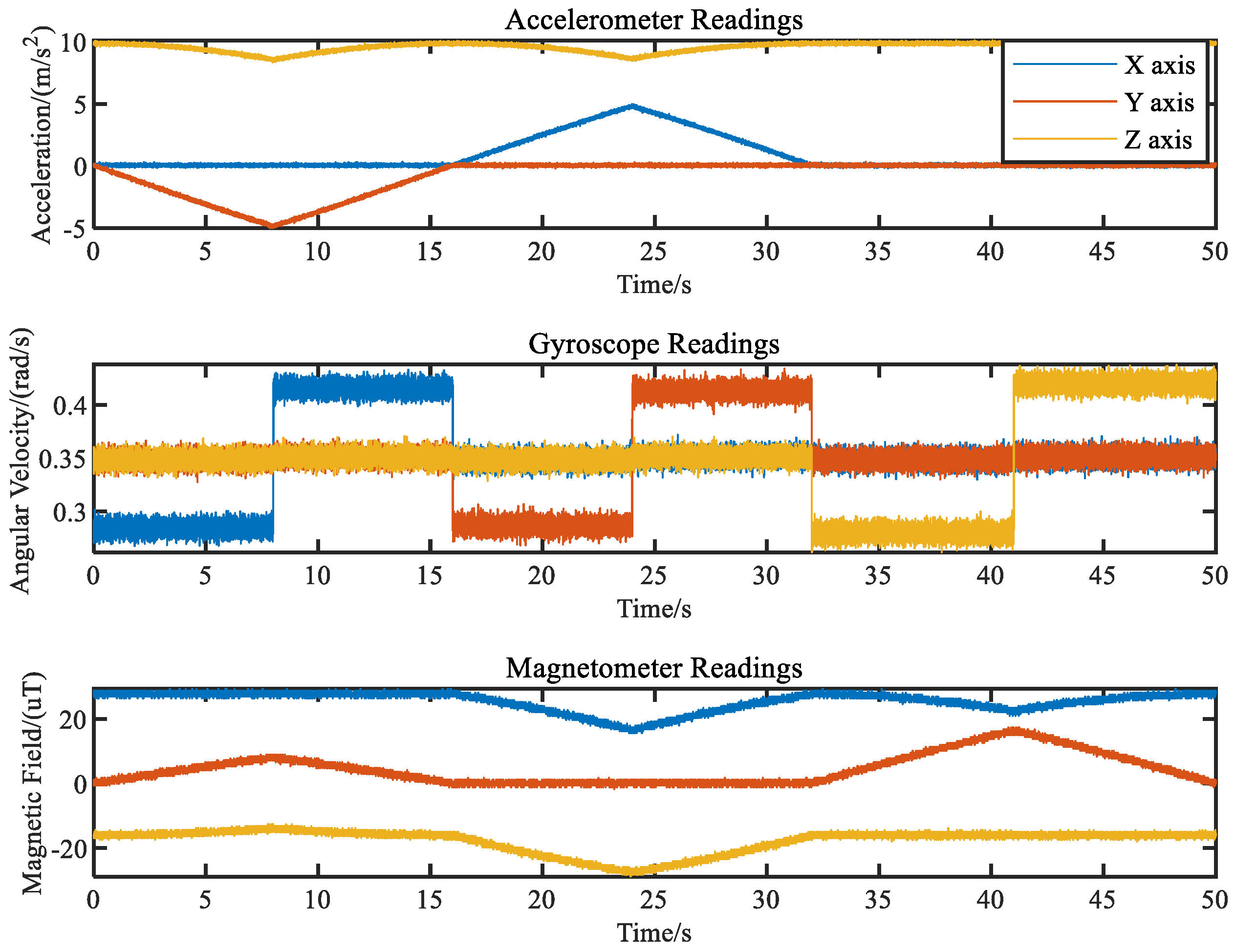
Assuming the flight trajectory of the UAV is as shown in Figure 7, the MARG data output by the MPU9250 sensor are shown in Figure 8. The attitude angles are calculated using the Madgwick algorithm from the MARG data, and the curve of the attitude angle errors is shown in Figure 9. It can be seen from Figure 9 that the systematic error of the UAV’s attitude angles during flight is not always fixed, but varies with time.

In this simulation, the navigation positioning method utilized estimated attitude angle data of the UAV, whereas the static method employed actual attitude angle data as shown in Figure 9. The total simulation time was 100 s, and the other conditions were the same as those in 6.1(a); the simulation results are shown in Figure 10 and

Table 5. RMSE of the target position under time-varying attitude errors.

Method	RMSE of the Target Position (m)
The navigation positioning method	955.07
The attitude correction method	232.57
The static method	355.12

.

As shown in Figure 10, the estimated target state of the navigation positioning method cannot converge, and it exhibits significant fluctuations. A comparison with the target state estimated by the static method reveals that this is attributable to systematic errors in the time-varying attitude angles. When the systematic errors of the attitude angle are substantial, the navigation positioning method yields less accurate estimations of the target state. Conversely, when these errors are relatively minor, the target state estimation improves.

In addition, the target state estimated by the attitude correction algorithm is similar to that estimated by the static method, and it is closer to the true target state. Further quantitative analysis of the results in Table 5 shows that the target state estimated by the attitude correction method is superior to the static method. The simulation results verify that the attitude correction algorithm proposed in this paper can effectively reduce the impact of time-varying attitude angle deviation on positioning accuracy, and it also rectifies a portion of the systematic error originating from the sensor observation.

In summary, compared with the existing error registration algorithms of inertial platform sensor systems, the proposed attitude correction algorithm can avoid establishing the state equation of attitude angle systematic errors, thus overcoming the influence of time-varying attitude angle systematic errors on the positioning accuracy. Moreover, the proposed algorithm has a simple principle, a small calculation amount, and easy real-time online processing, making it suitable for engineering applications.

(d)

The impact of observation target error on the attitude correction algorithm

As seen in Section 6.1(c), the attitude correction algorithm can reduce a portion of the systematic error originating from the sensor observation and improve the positioning accuracy of the target. Therefore, this section analyzes the impact of the systematic error originating from the sensor observation on the attitude correction algorithm. The parameters of the observation target error by the UAV are displayed in

Table 6. Values of target angle measurement errors (°).

Group of Angle Measurement Errors	1	2	3	4
System error	0.01	0.05	0.1	0.2
Random error	0.2	0.2	0.2	0.2

(set azimuth and elevation to the same error), and the other conditions were the same as those in 6.1(a); the simulation results are shown in

Table 7. RMSE of the target position under different target angle measurement errors.

Group of Angle Measurement Errors	RMSE of the Target Position under Different Methods (m)
	The Navigation Positioning Method	The Attitude Correction Method	The Static Method
1	268.31	69.21	55.39
2	393.88	142.80	174.06
3	546.23	292.48	324.51
4	882.90	627.08	659.21

.

An analysis of the data presented in columns 3 and 4 of Table 7 reveals that when the measurement error of the UAVs’ observation of the target is relatively small, the target localization accuracy of the attitude correction method significantly surpasses that of the navigation positioning method. In the case where the measurement error of the UAV’s observation the target increases to a certain extent, although the attitude angle error of the UAVs is not the predominant factor affecting localization accuracy, the attitude correction method can correct part of the observation system error of the UAVs, resulting in a higher target positioning accuracy compared to the static method. Through the analysis of the data in the fourth group, it can be observed that when there is substantial systematic error in the UAVs’ observation of the target, the improvement in target localization accuracy offered by the attitude correction algorithm is not substantial.

6.2. Multi-UAVs Cooperative Target Tracking and Trajectory Optimization

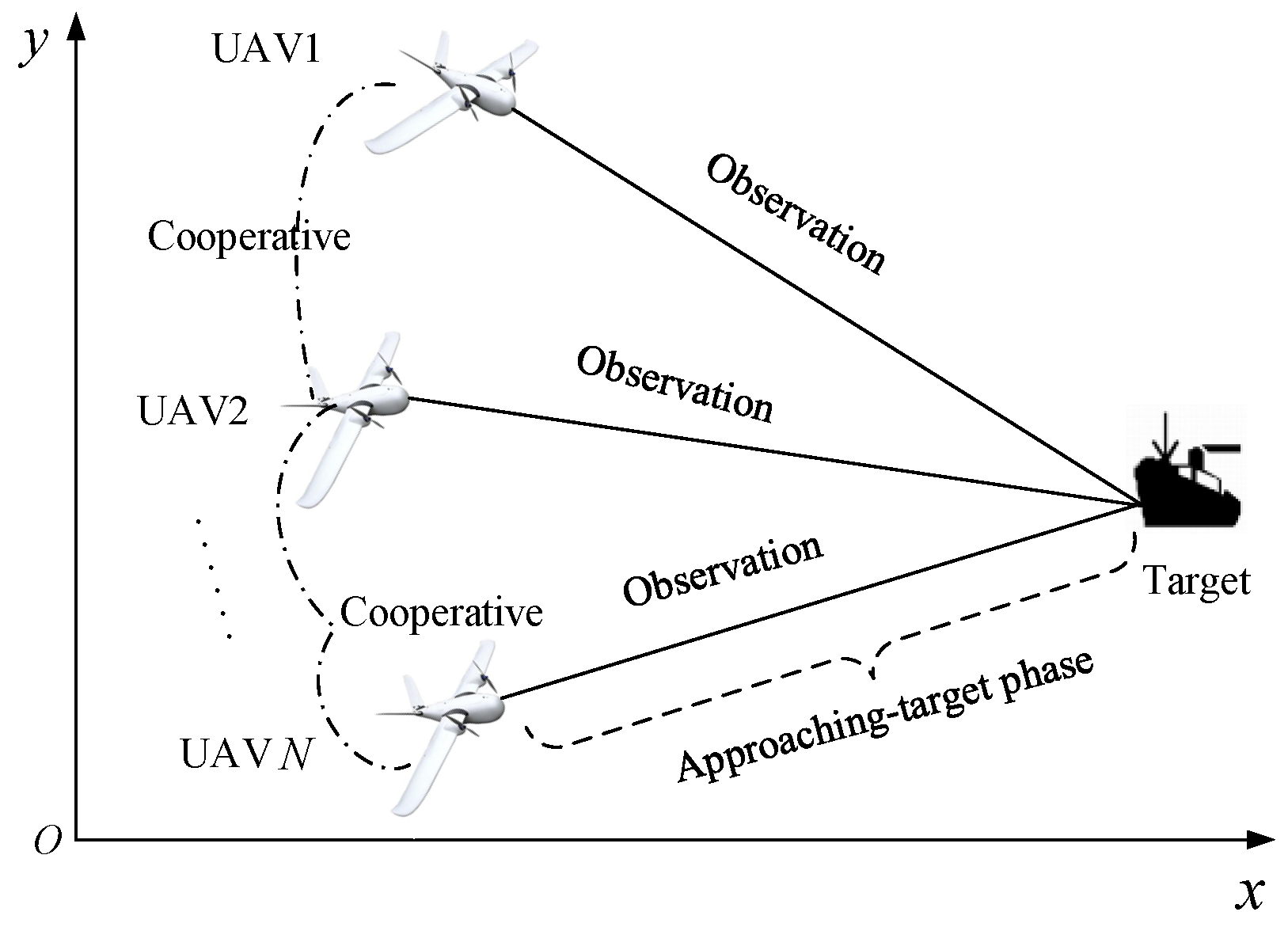
This section reports the simulation experiments conducted to verify the effectiveness of the proposed algorithm based on the attitude correction method when muti-UAVs track the maneuvering target. The simulation parameters were set as follows: the cooperation platform was located at (0 m, 0 m, 0 m), with both the UAVs and the cooperative platform at a distance of 20 km. The UAVs flew at a fixed altitude, and the initial positions and performance parameters of the three UAVs are shown in

Table 8. Initial state and performance parameters of UAVs.

Number	Initial State	${\mathit{v}}_0$	$\mathbf{\Delta }{\mathit{v}}_{\mathbf{max}}$	${\mathit{\omega }}_{\mathbf{max}}$
UAV1	(16,200 m, 11,700 m, 2000 m)	100 m/s	10 m/s	0.35 rad/s
UAV2	(11,700 m, 16,200 m, 2000 m)	100 m/s	10 m/s	0.35 rad/s
UAV3	(13,950 m, 13,950 m, 2000 m)	100 m/s	10 m/s	0.35 rad/s

. The errors of the UAV’s observation of the target and cooperation platform are shown in

Table 9. Values of UAV observation.

Type of the Error	System Error	Random Error
The error of the UAVs’ observation of the cooperation platform	(5 m, 0.03°, 0.03°)	(5 m, 0.2°, 0.2°)
The error of the UAVs’ observation of the target	(5 m, 0.03°, 0.03°)	(5 m, 0.2°, 0.2°)

. The target with the initial state of ${\mathit{X}}_t={\left[95 \mathrm{km},10 \mathrm{m}/\mathrm{s},95 \mathrm{km},10 \mathrm{m}/\mathrm{s},0 \mathrm{m},0 \mathrm{m}/\mathrm{s}\right]}^T$ performed right-turn maneuvering of 0.2°/s in 350 s~650 s, performed left-turn maneuvering of 0.2°/s in 850 s~1150 s, and maintained a uniform motion for the rest of the time. The initial situation of the cooperation platform, target, and UAVs are shown in Figure 11, and the total simulation time is 1500 s with a simulation interval of 0.5 s.

Under the target maneuvering conditions mentioned above, the IMM algorithm uses three models to estimate the state: uniform motion model, acceleration model, and turning model. The initial values of the model probability $\mathsf{\mu }=[0.3 0.3 0.4]$, and the state transition matrix is

$$\mathbf{\Pi }=\left[\begin{array}{ccc}0.95& 0.025& 0.025\\ 0.025& 0.95& 0.025\\ 0.025& 0.025& 0.95\end{array}\right]$$

The initial control sequence for the RHO method is ${\mathrm{U}0=[100,0;100,0;100,0;100,0;100,0;100,0;100,0;100,0;100,0]}^T$, and the relevant simulation parameters are shown in

Table 10. Simulation parameters of RHO method.

Parameter	Value	Unit
Predicted steps $N_p$	9	N/A
Delay constant ${\tau }_v$, ${\tau }_{\omega }$	0.5	s
Penalty factor ${\mu }_c$, ${\mu }_w$	1 × 105	N/A
Termination threshold $\epsilon$	0.001	N/A
Initial iteration step size $\Delta$	0.05	N/A
Factor of step size $\alpha$	0.9	N/A

.

(a)

Scenario 1 of cooperative target tracking

This section discusses the situation of the cooperative target tracking by UAV1 and UAV2. The systematic errors and random errors of the UAVs’ attitude angles are both (0.1°, 0.1°, 0.1°). Using the cooperative target tracking and trajectory optimization presented in Section 5, the simulation results are shown in Figure 12, Figure 13, Figure 14, Figure 15 and Figure 16.

Figure 12 shows the trajectory of the UAVs optimized by the RHO method, and Figure 13 depicts the variation curve of the line of sight between the UAVs and the target. It can be seen that for the maneuvering target, the line of sight between two UAVs and the target approaches 90 degrees, indicating that the UAVs are in an optimized observation position. This is consistent with a previous theoretical analysis [43], demonstrating the effective optimization of the UAVs’ trajectory using the RHO method.

The estimated trajectories of the maneuvering target are presented in Figure 14. It can be seen from Figure 14 that the target trajectory estimated by a single UAV without the attitude correction algorithm deviates greatly from the real target trajectory, while the trajectory estimated by a single UAV with the attitude correction algorithm is relatively close to the real target trajectory. Compared with the single UAV’s observation, the target trajectory of two UAVs’ cooperative estimation based on the attitude correction algorithm is closer to the real trajectory. Figure 15 and Figure 16 show the RMSE of the target position and velocity after 200 Monte Carlo simulations, respectively. As shown in Figure 15 and Figure 16, the fusion of the estimation algorithms of two UAVs based on the attitude correction algorithm can significantly improve the tracking accuracy. The comparison parameters in

Table 11. Performance comparison result of the three algorithms.

	Algorithm	The Navigation Positioning Method		The Attitude Correction Method		Fusion Estimate of Two UAVs with Attitude Correction Method
RMSE		UAV1	UAV2	UAV1	UAV2
RMSE of position (m)		361.9	408.6	110.5	118.9	19.8
RMSE of velocity (m/s)		3.76	3.99	3.79	3.31	2.09

also confirm this conclusion.

(b)

Scenario 2 of cooperative target tracking

To illustrate the adaptability of the algorithm, this section reports a simulation conducted to examine the effectiveness of the fusion estimation algorithm of two UAVs based on the attitude correction proposed in this paper when the attitude angle error is large. The systematic error and random error of the UAVs’ attitude angles were both (0.2°, 0.2°, 0.2°), and the remaining simulation parameters were the same as those of Section 6.2(a). The simulation results are shown in Figure 17, Figure 18 and Figure 19 and

Table 12. Performance comparison result of the algorithm with large attitude angle error.

	Algorithm	The Navigation Positioning Method		The Attitude Correction Method		Fusion Estimate of Two UAVs with Attitude Correction Method
RMSE		UAV1	UAV2	UAV1	UAV2
RMSE of position (m)		715.2	772.2	110.1	114.8	24.1
RMSE of velocity (m/s)		5.92	5.53	3.85	4.17	2.35

.

As shown in Figure 17, Figure 18 and Figure 19 and Table 12, the attitude correction algorithm proposed in this paper can effectively improve the target location accuracy in the case of the large attitude angle errors. Moreover, compared to the results of the single UAV’s estimated target state based on the attitude correction algorithm, the fusion of the estimation algorithms of the two UAVs based on the attitude correction can significantly improve the target detection accuracy. By comparing Table 11 and Table 12, the target tracking accuracy obtained by the attitude correction algorithm under different attitude angle errors is almost consistent, indicating that the proposed algorithm can effectively eliminate the influence of attitude angle errors on tracking accuracy.

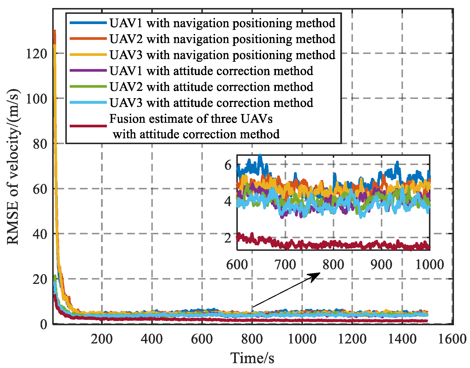
(c)

Scenario 3 of cooperative target tracking

To evaluate the effectiveness of the multi-UAV cooperative tracking algorithm, this section discusses the scenario in which UAV 1, UAV 2, and UAV 3 cooperatively tracked a target; UAV 3 was added based on the framework established in Section 6.2(b). The attitude angle system error and random error of UAV 3 were both (0.2°, 0.2°, 0.2°). The initial position and performance of UAV 3 are shown in

Table 13. Performance comparison result of the algorithm with three UAVs.

	Algorithm	The Navigation Positioning Method			The Attitude Correction Method			Fusion Estimate of Three UAVs with Attitude Correction Method
RMSE		UAV1	UAV2	UAV3	UAV1	UAV2	UAV3
RMSE of position (m)		726.1	779.6	743.3	110.7	118.1	108.8	22.5
RMSE of velocity (m/s)		5.82	5.61	5.49	3.81	4.20	3.94	1.91

. The other simulation parameters were consistent with those in 6.2(b), and the simulation results are shown in Figure 20, Figure 21, Figure 22, Figure 23, Figure 24 and Figure 25.

As shown in Figure 20, Figure 21 and Figure 22, the optimized UAV trajectory based on the RHO method allows for the UAV to form an optimized observation configuration under the condition of satisfying angular velocity constraints (as shown in Figure 21), where the line of sight between three UAVs and the target is maintained at 60 degrees or 120 degrees. This observation configuration is very conducive to cooperative detection.

Figure 23, Figure 24 and Figure 25 and Table 13 show that the proposed algorithm can effectively improve the detection accuracy. A comparison between Table 12 and Table 13 shows that, compared to the fusion estimation of two UAVs based on the attitude correction algorithm, the fusion estimation of three UAVs increases the position accuracy of the target from 24.1 m to 22.5 m and the velocity accuracy from 2.35 m/s to 1.91 m/s. The detection accuracy is improved to a certain extent, but the improvement is not significant.

In summary, combining Section 6.2(a), Section 6.2(b), and Section 6.2(c) shows that the proposed algorithm can effectively optimize the observation trajectory of the UAV, reduce the influence of UAV attitude angle errors on observation accuracy, and improve the cooperative tracking accuracy of the target. The simulation results verify the effectiveness of the proposed method.

7. Conclusions

The multi-UAVs cooperative target tracking capabilities depend not only on reducing the observation error of the UAV on the target, but also on reducing the attitude angle error of the UAV. To enhance the tracking accuracy of a remote maritime target, this paper proposes a multi-UAVs cooperative target tracking method based on the attitude correction algorithm.

(1)

Based on the precise position of the cooperative platform, the attitude correction algorithm is proposed, which can not only reduce the attitude angle error of the UAV, but also reduce the observation system error of the UAV with the support of a high-precision cooperative platform location. This algorithm has the advantages of a small computational complexity and good real-time performance, making it suitable for engineering applications.

(2)

The multi-UAVs cooperative tracking is realized by combining the effective filtering algorithm with the trajectory optimization method. In this paper, a cooperative trajectory optimization algorithm for multi-UAVs based on a cooperative platform is proposed by combining the improved RHO algorithm and the attitude correction algorithm.

(3)

The simulation results show that the multi-UAVs target tracking algorithm based on the attitude correction method can effectively reduce the attitude angle error and observation error of the UAV. Meanwhile, the proposed multi-UAVs cooperative trajectory optimization method can improve the quality of the target observation information, thereby enhancing the tracking accuracy of the remote maritime target. The results of this study can provide valuable references for multi-UAVs cooperative detection.

In fact, the relative positions of the cooperative platform, the target, and the UAV have an impact on the attitude correction algorithm. This study simply planned the trajectory of the cooperative platform, and the results of the attitude correction algorithm may not be optimal. Furthermore, the trajectory optimization algorithm employed in this study is sensitive to initial values and lacks robustness. Investigating the optimal configuration of the cooperative platform, the target, and the UAV, and improving the robustness of the trajectory optimization algorithm are the directions of our efforts. Additionally, future research will focus on high-precision maneuvering target filtering algorithms and the implementation of multi-targets tracking by multi-UAVs.

References

1. He, S.; Shin, H.; Tsourdos, A. Trajectory optimization for multitarget tracking using joint probabilistic data association filter. J. Guid. Control Dyn. 2020, 43, 170–178. [Google Scholar] [CrossRef]
2. Fonod, R.; Shima, T. Estimation enhancement by cooperatively imposing relative intercept angles. J. Guid. Control Dyn. 2017, 40, 1711–1725. [Google Scholar] [CrossRef]
3. Kottath, R.; Narkhede, P.; Kumar, V.; Karar, V.; Poddar, S. Multiple model adaptive complementary filter for attitude estimation. Aerosp. Sci. Technol. 2017, 69, 574–581. [Google Scholar] [CrossRef]
4. Li, Y.; Qi, G.; Sheng, A. Optimal deployment of vehicles with circular formation for bearings-only multi-target localization. Automatica 2019, 105, 347–355. [Google Scholar] [CrossRef]
5. Xu, S.; Rice, M.; Rice, F. Optimal TOA-sensor placement for two target localization simultaneously using shared sensors. IEEE Commun. Lett. 2021, 25, 2584–2588. [Google Scholar] [CrossRef]
6. Cui, Y.; Song, Q.; He, Y. A modified exact method-based mobile radar registration algorithm. J. Astronaut. 2011, 32, 903–910. [Google Scholar]
7. Cui, Y.; Xiong, W.; He, Y. Mobile platform sensor registration algorithm based on MLR. Acta Aeronaut. Astronaut. Sin. 2012, 33, 118–128. [Google Scholar]
8. Cheng, R.; Heng, K. Augment State Registration Algorithm Based on CKF. Aeronaut. Sci. Technol. 2018, 29, 66–73. [Google Scholar]
9. Xiong, W.; Pan, X.; Peng, Y.; He, Y. Unscented Bias Estimation Technique for Maneuvering Sensor. Acta Aeronaut. Astronaut. Sin. 2010, 31, 819–824. [Google Scholar]
10. Xiong, W.; Xing, F.; Pan, X.; Peng, Y. Bias estimation for moving sensors network using cooperation targets. Syst. Eng. Electron. 2011, 33, 544–547. [Google Scholar]
11. Wang, G.; Chen, L.; Jia, S. Optimized bias estimation model for 3-D radar considering platform attitude errors. IEEE Aerosp. Electron. Syst. Mag. 2012, 27, 19–24. [Google Scholar] [CrossRef]
12. Chen, L.; Wang, G.; Jia, S.; Progri, I. Attitude bias conversion model for mobile radar error registration. J. Navig. 2012, 65, 651–670. [Google Scholar] [CrossRef]
13. Wang, Y.; Zheng, W.; Sun, S.; Li, L. Robust information filter based on maximum correntropy criterion. J. Guid. Control Dyn. 2016, 39, 1126–1131. [Google Scholar] [CrossRef]
14. Xie, G.; Sun, L.; Wen, T.; He, X.; Qian, F. Adaptive transition probability matrix-based parallel IMM algorithm. IEEE Trans. Syst. Man Cybern. Syst. 2021, 51, 2980–2989. [Google Scholar] [CrossRef]
15. Frew, E.; Lawrence, D.; Morris, S. Coordinated standoff tracking of moving targets using Lyapunov guidance vector fields. J. Guid. Control Dyn. 2008, 31, 290–306. [Google Scholar] [CrossRef]
16. Lawrence, D.; Frew, E.; Pisano, W. Lyapunov vector fields for autonomous UAV flight control. J. Guid. Control Dyn. 2008, 31, 1220–1229. [Google Scholar] [CrossRef]
17. Yao, P.; Wang, H.; Su, Z. Cooperative path planning with applications to target tracking and obstacle avoidance for multi-UAVs. Aerosp. Sci. Technol. 2016, 54, 10–22. [Google Scholar] [CrossRef]
18. Chen, H.; Chang, K.; Agate, C. UAV path planning with tangentplus-Lyapunov vector field guidance and obstacle avoidance. IEEE Trans. Aerosp. Electron. Syst. 2013, 49, 840–856. [Google Scholar] [CrossRef]
19. Lim, S.; Kim, Y.; Lee, D.; Bang, H. Standoff target tracking using a vector field for multiple unmanned aircrafts. J. Intell. Robot. Syst. 2013, 69, 347–360. [Google Scholar] [CrossRef]
20. Zhao, S.; Chen, B.; Tong, H. Optimal deployment of mobile sensors for target tracking in 2D and 3D spaces. IEEE/CAA J. Autom. Sin. 2015, 1, 24–30. [Google Scholar]
21. Song, Z.; Li, H.; Chen, C.; Zhou, X.; Xu, F. Coordinated standoff tracking of moving targets using differential geometry. J. Zhejiang Univ. Sci. C. 2014, 15, 284–292. [Google Scholar] [CrossRef]
22. Yao, P.; Wang, H.; Su, Z. Real-time path planning of unmanned aerial vehicle for target tracking and obstacle avoidance in complex dynamic environment. Aerosp. Sci. Technol. 2015, 47, 269–279. [Google Scholar] [CrossRef]
23. Kokolakis, N.; Koussoulas, N. Robust standoff target tracking with finite-time phase separation under unknown wind. J. Guid. Control Dyn. 2021, 44, 1183–1198. [Google Scholar] [CrossRef]
24. Liu, Z.; Xang, L.; Zhu, Z. Cooperative Standoff Target Tracking using Multiple Fixed-Wing UAVs with Input Constraints in Unknown Wind. Drones 2023, 7, 593. [Google Scholar] [CrossRef]
25. Li, B.; Song, C.; Bai, S.; Huang, J.; Ma, R.; Wan, K.; Neretin, E. Multi-UAV trajectory planning during cooperative tracking based on a Fusion Algorithm integrating MPC and standoff. Drones 2023, 7, 196. [Google Scholar] [CrossRef]
26. Lin, C.; Shi, J.; Zhang, W.; Lyu, Y. Standoff tracking of a ground target based on coordinated turning guidance law. ISA Trans. 2022, 119, 118–134. [Google Scholar] [CrossRef] [PubMed]
27. Du, B.; Yang, K.; Zhang, W.; Chen, H. Terminal line-of-sight angle-constrained target tracking guidance for unmanned surface vehicles. IEEE Trans. Veh. Technol. 2024, 73, 1–15. [Google Scholar] [CrossRef]
28. Wang, Z.; Xu, G.; Long, T. Customized interior-point method for cooperative trajectory planning of unmanned aerial vehicles. Acta Autom. Sin. 2023, 49, 2374–2385. [Google Scholar]
29. Chai, R.; Savvaris, A.; Tsourdos, A.; Chai, S.; Xia, Y. Improved gradient-based algorithm for solving aeroassisted vehicle trajectory optimization problems. J. Guid. Control Dyn. 2017, 40, 2091–2099. [Google Scholar] [CrossRef]
30. Zhang, Z.; Li, J.; Wang, J. Sequential convex programming for nonlinear optimal control problems in UAV path planning. Aerosp. Sci. Technol. 2018, 76, 280–290. [Google Scholar] [CrossRef]
31. Zhou, H.; Cai, Z.; Zhao, J.; Wang, Y. RHO-based convex optimization method applied to cooperative trajectory planning for multiple UAVs. In Proceedings of the 2017 Asian Control Conference (ASCC), Gold Coast, Australia, 17–20 December 2017; pp. 1572–1577. [Google Scholar]
32. Meng, Q.; Chen, K.; Qu, Q. PPSwarm: Multi-UAV path planning based on hybrid PSO in complex scenarios. Drones 2024, 8, 192. [Google Scholar] [CrossRef]
33. Cui, N.; Guo, D.; Li, K.; Wei, C. A survey of numerical methods for aircraft trajectory optimization. Tact. Missile Technol. 2020, 5, 37–51. [Google Scholar]
34. Di, B.; Zhou, R.; Duan, H. Potential field based receding horizon motion planning for centrality-aware multiple UAV cooperative surveillance. Aerosp. Sci. Technol. 2015, 46, 386–397. [Google Scholar] [CrossRef]
35. Wang, Y.; Zhang, T.; Cai, Z.; Zhao, J.; Wu, K. Multi-UAV coordination control by chaotic grey wolf optimization based distributed MPC with event-triggered strategy. Chin. J. Aeronaut. 2020, 33, 2877–2897. [Google Scholar] [CrossRef]
36. Fabio, A. Constrained dynamic compensation with model predictive control for tracking. Aerosp. Sci. Technol. 2019, 93, 105340. [Google Scholar]
37. Zhang, S.; Guo, Y.; Lu, Z. Cooperative detection based on the adaptive interacting multiple model-information filtering algorithm. Aerosp. Sci. Technol. 2019, 93, 105310. [Google Scholar] [CrossRef]
38. Beck, F.; Vu, M.; Hartl, C.; Kugi, A. Model predictive trajectory optimization with dynamically changing waypoints for serial manipulators. IEEE Robot. Autom. Lett. 2024, 9, 6488–6495. [Google Scholar] [CrossRef]
39. Sun, L. Research and Application of Interacting Multiple Model Algorithm with Adaptive Transition Probability Matrix. Master’s Thesis, Xi’an University of Technology, Xi’an, China, 2019. [Google Scholar]
40. Kim, S.; Tadiparthi, V.; Bhattacharya, R. Computationally efficient attitude estimation with extended H2 filtering. J. Guid. Control Dyn. 2021, 44, 418–427. [Google Scholar] [CrossRef]
41. MPU-9250 Product Specification Revision 1.1. Available online: http://www.invensense.com/wp-content/uploads/2015/02/PS-MPU-9250A-01-v1.1.pdf (accessed on 20 June 2016).
42. Madgwick, S.; Harrison, A.; Vaidyanathan, R. Estimation of IMU and MARG orientation using a gradient descent algorithm. In Proceedings of the 2011 IEEE International Conference on Rehabilitation Robotics (ICORR), Zurich, Switzerland, 29 June–1 July 2011; pp. 1–7. [Google Scholar]
43. Zhao, S.; Chen, B.; Tong, H. Optimal sensor placement for target localization and tracking in 2D and 3D. Int. J. Control 2013, 86, 1687–1704. [Google Scholar] [CrossRef]
Figure 1. The scenario of multi-UAVs cooperative tracking in the approaching-target phase.
Drones 08 00405 g001
Figure 2. Schematic diagram of target localization based on attitude correction.
Drones 08 00405 g002
Figure 3. The control flow chart of multi-UAV trajectory optimization based on the RHO method.
Drones 08 00405 g003
Figure 4. Multi-UAVs cooperative tracking and trajectory optimization process.
Drones 08 00405 g004
Figure 5. State estimate of the target under different methods.
Drones 08 00405 g005
Figure 6. Simulation flow chat of attitude estimation.
Drones 08 00405 g006
Figure 7. True trajectories imported to MATLAB for simulation.
Drones 08 00405 g007
Figure 8. MARG data from MATLAB function imuSensor with MPU-9250.
Drones 08 00405 g008
Figure 9. The curve of attitude errors.
Drones 08 00405 g009
Figure 10. Trajectories of the target.
Drones 08 00405 g010
Figure 11. Initial location of simulation.
Drones 08 00405 g011
Figure 12. The trajectory of two UAVs and target.
Drones 08 00405 g012
Figure 13. The line of sight between two UAVs and target.
Drones 08 00405 g013
Figure 14. The trajectory of the estimate target with two UAVs.
Drones 08 00405 g014
Figure 15. The evolution of position’s RMSE with two UAVs.
Drones 08 00405 g015
Figure 16. The evolution of velocity’s RMSE with two UAVs.
Drones 08 00405 g016
Figure 17. The trajectory of the estimate target with large attitude angle error.
Drones 08 00405 g017
Figure 18. The evolution of position’s RMSE with large attitude angle error.
Drones 08 00405 g018
Figure 19. The evolution of velocity’s RMSE with large attitude angle error.
Drones 08 00405 g019
Figure 20. The trajectory of three UAVs and target.
Drones 08 00405 g020
Figure 21. The variation curve of the yaw rate.
Drones 08 00405 g021
Figure 22. The line of sight between three UAVs and target.
Drones 08 00405 g022
Figure 23. The trajectory of the estimate target with three UAVs.
Drones 08 00405 g023
Figure 24. The evolution of position’s RMSE with three UAVs.
Drones 08 00405 g024
Figure 25. The evolution of velocity’s RMSE with three UAVs.
Drones 08 00405 g025