Aerial Map-Based Navigation by Ground Object Pattern Matching

Abstract

This paper proposes a novel approach to map-based navigation for unmanned aircraft. The proposed approach employs pattern matching of ground objects, not feature-to-feature or image-to-image matching, between an aerial image and a map database. Deep learning-based object detection converts the ground objects into labeled points, and the objects’ configuration is used to find the corresponding location in the map database. Using the deep learning technique as a tool for extracting high-level features reduces the image-based localization problem to a pattern-matching problem. The pattern-matching algorithm proposed in this paper does not require altitude information or a camera model to estimate the horizontal geographical coordinates of the vehicle. Moreover, it requires significantly less storage because the map database is represented as a set of tuples, each consisting of a label, latitude, and longitude. Probabilistic data fusion with the inertial measurements by the Kalman filter is incorporated to deliver a comprehensive navigational solution. Flight experiments demonstrate the effectiveness of the proposed system in real-world environments. The map-based navigation system successfully provides the position estimates with RMSEs within 3.5 m at heights over 90 m without the aid of the GNSS.

1. Introduction

Most unmanned aircraft depend on the Global Navigation Satellite System (GNSS) to determine their position and speed while in flight. The GNSS is often employed to periodically adjust the inertial navigation system (INS), which calculates a vehicle’s present location and velocity by processing accumulated acceleration data over time. However, particularly in military contexts, issues such as jamming, interference, and accidental disruptions due to the shape of the terrain can lead the GNSS device to malfunction or cease operation. Numerous researchers are exploring alternative or complementary solutions to address the challenges faced in environments without the GNSS. These alternatives aim to manage the INS’s error buildup and offer precise positioning information in terms of latitude and longitude.

Database-referenced navigation (DBRN) offers a viable alternative to the GNSS, mitigating the dependency on external systems through an onboard database. The fundamental concept of DBRN involves identifying and matching surrounding geographical features with those cataloged in a geo-referenced database. A representative example of DBRN is terrain-aided navigation (TAN), also known as terrain-referenced navigation (TRN), which derives positioning information by matching radar altimeter readings of the ground’s elevation beneath an aircraft to a preloaded digital elevation model (DEM). TAN is considered a reliable choice because it can operate in all weather conditions at low flight altitudes over terrain, thanks to a radar altimeter. However, the applicability of the TAN system is somewhat restricted to scenarios where the use of costly, bulky altimetry and inertial sensors is feasible, such as in cruise missiles or large airplanes. Additionally, the TAN system’s primary challenges are attributed to the nature of radar altimeter measurements. Near the inflection points where the slope changes sign, the one-dimensional measurements suffer from ambiguity, which could cause filter degradation and divergence [1]. The broad beam of the radar altimeter necessarily causes a large error in slant range measurements [2].

An alternative method is vision-based navigation, which uses images captured by an aircraft’s camera to determine its position. This technique is appealing for two main reasons: first, cameras are passive sensors, making them difficult to detect or interfere with; and second, since most unmanned aircraft are already equipped with cameras, there is no need for additional equipment to leverage vision data for navigation. Early studies in vision-based navigation focused on deriving elevation data from aerial images and aligning these data with a DEM [3,4]. These methods can be seen as a two-dimensional enhancement of TAN. More recent research involves conducting a stereo analysis of image sequences to calculate the heights of feature points and compare these with the DEM to deduce the vehicle’s status [5]. Nevertheless, this vision-based TAN method has its limitations, as its effectiveness hinges on the DEM’s resolution and precision. Moreover, the actual visual terrain elevation may not match the DEM, typically generated using synthetic aperture radar (SAR). Therefore, careful development of the digital surface model (DSM), as in [6], is necessary to obtain an accurate elevation model of the visual terrain surface, ensuring more reliable navigation.

Recently, map-based navigation methods have gained interest due to the accessibility of public map databases that provide 2D representations of locations via aerial or satellite imagery. With these resources, map-based navigation technologies eliminate the need for a map-building process and can adapt to different aircraft systems and map databases. This study explores advancements in this emerging field.

1.1. Related Works

Various strategies have been explored to align images captured by aircraft-mounted cameras with these public maps, including image registration through correlation filters [7] and detecting and matching feature points between scenes [8]. Despite using feature descriptors like SURF [9], ORB [10] seems to be a viable solution. However, it has been verified that these methods do not guarantee the extraction of the same features from the aerial image and the satellite image [11]. Identifiable landscape features have often been used to characterize the scene. For example, mountain drainage patterns in satellite images were compared with those on a map using the wavelet transform, considering these patterns as a unique fingerprint of mountainous regions [12]. In [13], road intersections were used to match aerial images to a database. All possible permutations were accounted for to represent rotations of the road intersections. Nonetheless, challenges such as changes in scale, orientation, and lighting conditions complicate these vision-based methods. Additionally, the infrequent and inconsistent updates of public map databases mean that recorded aerial images might not align due to seasonal variations. Consequently, deep learning methods have been employed to extract semantic segments from aerial images [11,14,15]. These segments are known to be less sensitive to variations in low-level features that can be inconsistent in heterogeneous imagery sources. Recent studies [11,15] have demonstrated the viability of map-based navigation by representing each semantic segment with a unique descriptor. Each semantic segment is considered a distinctive feature, and map matching is conducted by comparing the descriptor values of the features in the aerial images with those in the map database.

1.2. Contributions

While recent approaches attempt to use deep learning techniques as feature detectors, this paper introduces a map-based navigation system that further abstracts ground objects in aerial images into points. The proposed method, based on the strategy outlined in a research note [14], uses deep learning technologies to extract high-level features from aerial images and a map database. For example, once ground objects such as road intersections, buildings, and highways are distinguished but not necessarily identified, the configuration of the objects can be used to find the corresponding location of the vehicle in the map database. In other words, aerial localization is performed by pattern matching of labeled objects, not feature-to-feature or image-to-image matching.

The pattern-matching algorithm proposed in this study compares the configuration of the objects in the aerial image with those in the database to determine the vehicle’s location. The output of the image processing is called a ‘meta image’, where the detected objects from an image are represented as points. Each point is represented as a tuple containing pixel coordinates of the object and its label. The map database is also represented as a meta image with geographical coordinates before being loaded onto the unmanned aircraft. This approach offers several advantages over existing methods. First, it significantly reduces the storage space and computational burden. Additionally, the pattern-matching algorithm does not require camera parameters, height above ground, and camera orientation. In other words, map matching is not affected by changes in the rotation and scale of the aerial images.

Ultimately, the proposed map-based navigation system incorporates fusion with the INS, providing a comprehensive navigational solution.

1.3. Outline

The key ideas of the proposed map-based navigation system are addressed in detail in Section 2. How to train and use the deep learning model for ground object detection and meta-image generation is discussed in Section 2.1. Then, the pattern-matching algorithm determines the vehicle’s location by identifying where the meta image corresponds within the database, as described in Section 2.2. The probabilistic filtering algorithm in Section 2.3 takes the localization result as the position measurement and fuses it with inertial measurements to provide stable, frequent estimates of position and velocity. Flight experiments demonstrate the effectiveness of the proposed map-based navigation system in real-world environments. The results of the flight experiments are discussed in Section 3. Finally, Section 4 provides a summary and the conclusions.

2. Proposed Map-Based Navigation System

A block diagram of the proposed map-based navigation system is presented in Figure 1. The overall system consists of image processing, pattern matching, an attitude and heading reference system (AHRS), and probabilistic data fusion blocks. The output of this system represents the primary aircraft states: position, velocity, and attitude. The output of image processing, called a meta image, is given to the map-matching block for comparison with the map database to determine the position of the camera. The position identified by the map-matching process is used as a measurement in the probabilistic data fusion block. The probabilistic data fusion block recursively estimates position and velocity using the map-based position measurement and the acceleration from the AHRS module. Note that the map-based navigation method discussed in this paper is limited to estimating the horizontal position, excluding vertical position estimation from its scope. The vertical position is assumed to be obtained through other means, such as barometric or radio altimeters.

Figure 2 illustrates the central concept of the proposed approach. The image-processing block uses a deep learning model to detect objects in the aerial image. The information required by the pattern-matching algorithm from the image is a set of tuples, each containing the type, or label, of the detected object and its pixel coordinates, which is referred to as a meta image in this study. The map database is also represented in the form of a meta image by executing object detection on the original map image in the same manner as for the aerial image. The difference is that the map database contains geographical coordinates of labeled ground objects. The pattern-matching algorithm identifies the location where the center of the image corresponds within the map database. The image processing and map-matching algorithm are discussed in detail in Section 2.1 and Section 2.2.

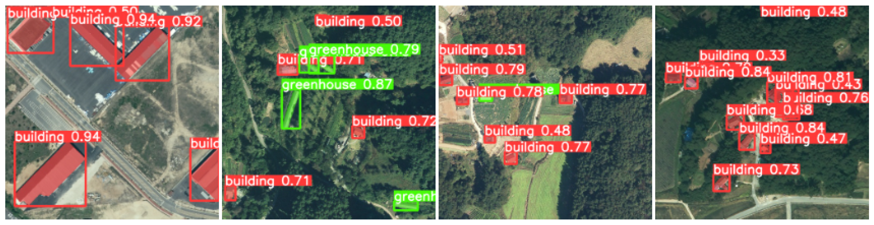
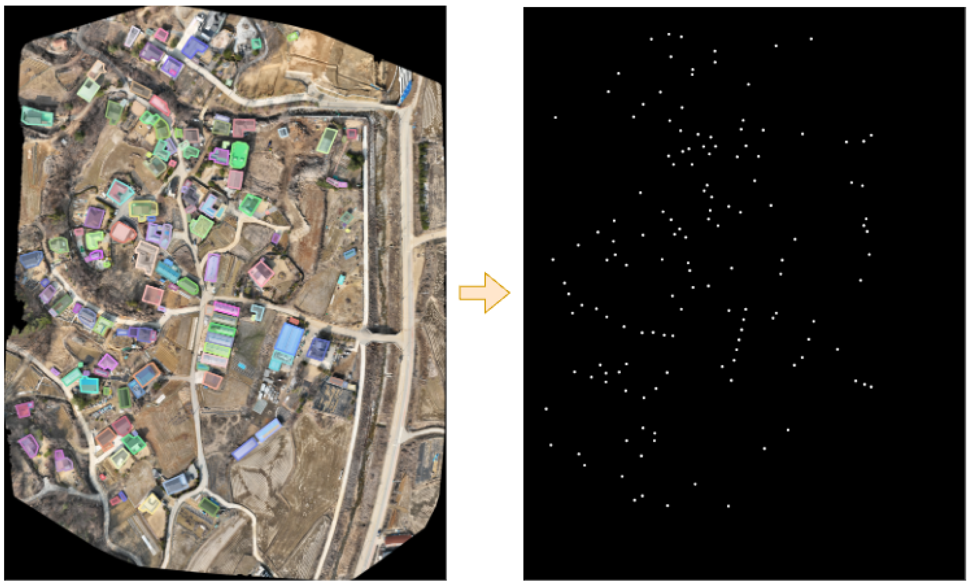
2.1. Image Processing

The image-processing block is designed to detect ground objects and represent them as labeled points. Each ground object can be designated a label, such as building, stadium, park or green area, road intersection, lake or river, agricultural field, or mountain. These ground objects are very robust in preserving their shape. Recognizing stationary ground objects from aerial images using traditional image-processing techniques is a challenging task. Each ground object has diverse-colored roofs and irregular shapes, with various types such as houses, apartments, greenhouses, warehouses, etc., making it difficult to clearly define the object of interest. A deep learning approach can facilitate the recognition of buildings in such ground data by learning directly from the data and classifying the recognized objects. Compared to traditional feature-based approaches, this method simplifies the re-identification of the same object from different viewpoints. In the realm of real-time object recognition in image data, research spans various methods, from two-stage techniques, such as R-CNN [16], Fast R-CNN [17], Faster R-CNN [18], and Mask R-CNN [19], to one-stage methods like SSD [20] and YOLO [21].

Given that object detection techniques often face challenges in accurately identifying rotated objects, we propose that instance segmentation serves as a suitable method for detecting objects and differentiating between them. Consequently, this approach enables the generation of image-processing outputs essential for the map-matching process. In this study, YOLOv7-seg [21], one of the latest open-source models, is used to perform instance segmentation. By using this model, the pixel coordinates of objects in each image are determined and passed to the pattern-matching algorithm described later.

Our model is currently trained to detect only buildings and greenhouses, serving as a proof of concept for the proposed method. Buildings and greenhouses are commonly found in rural areas where we demonstrate our system, and they are of appropriate size when captured during flight. The model’s functionality can be expanded to include various object types, enabling our system to address a broader range of geographical locations.

2.1.1. Dataset

For training, we utilized aerial image data from the Land Cover Map Aerial Satellite Image Dataset provided by AIHub [22]. This dataset contains aerial images covering various categories, including buildings, parking lots, roads, trees, fields, greenhouses, farmland, and more. Additional classification tasks or dataset augmentation can support more diverse object recognition. We specifically defined buildings and greenhouses from this dataset as ground structures and used them for training. Further details and the format of the dataset can be found in Figure 3 and

Table 1. Aerial image dataset configuration.

Meters per Pixel	Resolution	The Number of Images
0.25 m/pixel	$512\times 512$	50,000
0.25 m/pixel	$1024\times 1024$	5000
0.12 m/pixel	$512\times 512$	1000

.

2.1.2. Training and Validation

The dataset was split into training and validation sets in a ratio of 8:2. The YOLOv7-seg model was employed for training, utilizing four RTX3090 GPUs for 100 epochs. Transfer learning was performed from pre-trained weights on the Coco dataset, using stochastic gradient descent (SGD) for optimization. The learning rate started at 0.001 and decreased to 0.0001 during training. The training results and example images can be observed in

Table 2. Training results of YOLOv7-seg.

Class	Precision	Recall	mAP0.5	mAP0.5:0.95
All	0.857	0.768	0.614	0.845
Building	0.886	0.745	0.618	0.857
Greenhouse	0.828	0.791	0.611	0.833

and Figure 4.

Based on the image segmentation results, the center points of the detected objects were identified and passed through filtering before being forwarded to the pattern-matching algorithm. Figure 5 illustrates the image-processing results on images acquired during actual flights.

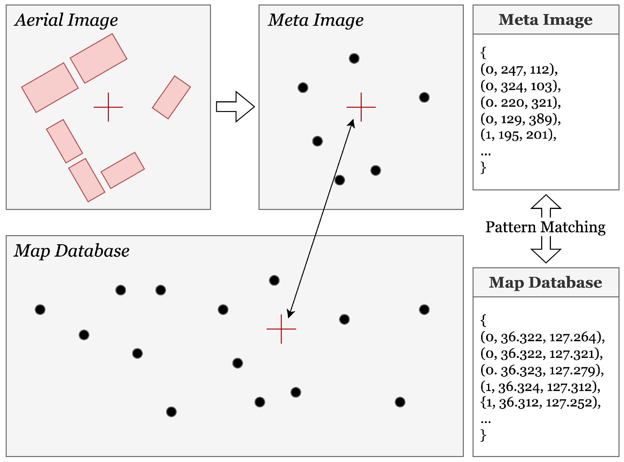
2.2. Localization by Map Matching

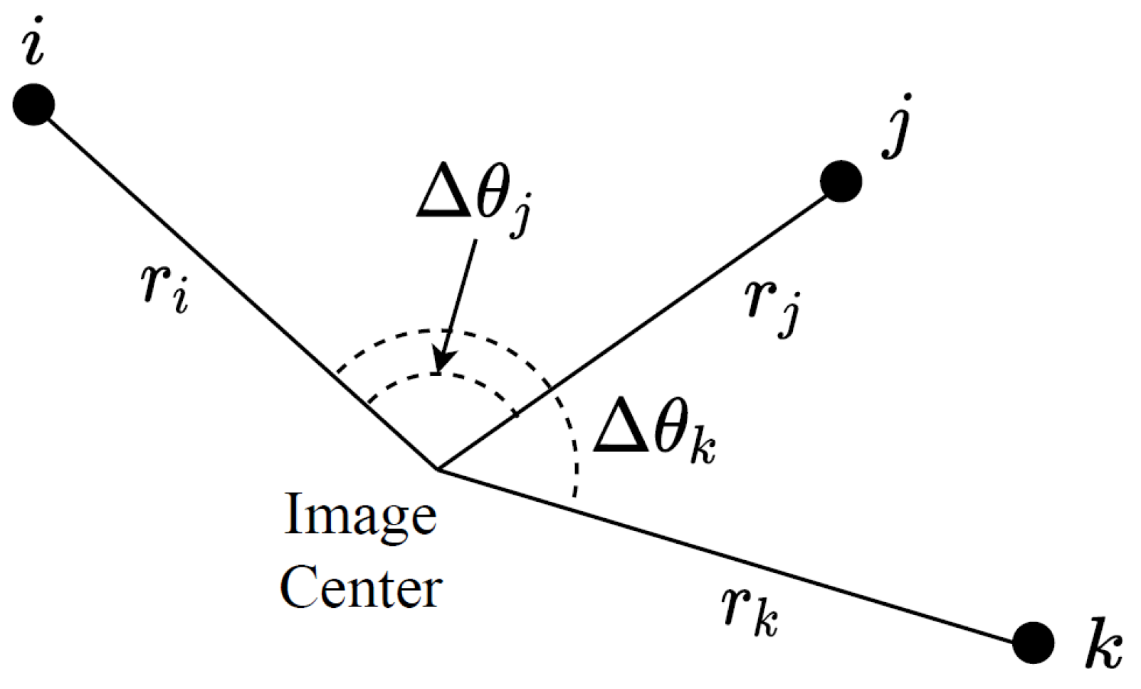
2.2.1. Pattern-Matching Algorithm

The purpose of the pattern-matching algorithm is to locate the center of the image on the map database and obtain its geographical coordinates. A set of pixel coordinates of the detected objects in an aerial image, called a meta image, is given as input to the pattern-matching algorithm. The algorithm also refers to the map database in the form of a meta image containing the geographical coordinates of ground objects. Here, a random sample consensus (RANSAC) [23]-based method is proposed in Algorithm 1. The consensus algorithm iteratively tests hypotheses of matching between the objects in an image and those in the database to provide one or multiple position candidates.

Suppose objects in the image and the database are denoted as $o^I$ and $o^D$, respectively. Each object has a label and a two-dimensional position in its own coordinate system. Given the two image objects $(o_i^I,o_j^I)$, we calculate their polar coordinates $(r_i,{\theta }_i)$ and $(r_j,{\theta }_j)$, with respect to the image center. Suppose two database objects $(o_i^D,o_j^D)$ have the same polar coordinates $(R_i,{\mathsf{\Theta }}_i)$ and $(R_j,{\mathsf{\Theta }}_j)$ with respect to some position in the database. In this case, the position becomes the position candidate. Comparing the polar coordinates is impractical because the units in the image and database are different. It is not guaranteed that the image is aligned with the database. Therefore, we employ the relative radius, $r_j/r_i$, and the relative angle, $\Delta {\theta }_j={\theta }_j-{\theta }_i$, to compare the two configurations in the different coordinate systems. This approach makes the pattern-matching process invariant to scale and rotation.

Algorithm 1 Proposed pattern-matching algorithm

1: for$(o_i^I,o_j^I)\in C\left(O^I\right)$do 2:     Calculate polar coordinates: $(r_i,{\theta }_i),(r_j,{\theta }_j)$ 3:     for $(o_i^D,o_j^D)\in P\left(O^D\right)$ if $label(o_i^D,o_j^D)=label(o_i^I,o_j^I)$ do 4:         Find the position candidate, $c_{ij}^D$, by Algorithm 2,         as one of the intersections of circles         centered at  $(o_i^D,o_j^D)$  with radii  $R_i:R_j=r_i:r_j$ 5:         $N_{matched}\leftarrow 2$ 6:         for $o_k^I\in O^I-\{o_i^I,o_j^I\}$ do 7:               Calculate polar coordinates: $(r_k,{\theta }_k)$ 8:               Calculate relative angle: $r_k/r_i$ 9:               Calculate relative radius: $\Delta {\theta }_k={\theta }_k-{\theta }_i$ 10:              for $o_k^D\in O^D-\{o_i^D,o_j^D\}$ if $label\left(o_k^D\right)=label\left(o_k^I\right)$ do 11:                    Calculate $(R_k,{\mathsf{\Theta }}_k)$ and therefore $R_k/R_i,\Delta {\mathsf{\Theta }}_k$ 12:                    if $|r_k/r_i-R_k/R_i|<{\delta }_r$ and $|\Delta {\theta }_k-\Delta {\mathsf{\Theta }}_k|<{\delta }_{\theta }$ then 13:                          $e_k\leftarrow |r_k/r_i-R_k/R_i|+|\Delta {\theta }_k-\Delta {\mathsf{\Theta }}_k|$ 14:                          $N_{matched}\leftarrow N_{matched}+1$ 15:           if $N_{matched}>=N_{min}$ then 16:                $E_{ij}\leftarrow std\left(\left\{e_k\right\}\right)$ 17:                $C^D\leftarrow C^D\cup c_{ij}^D$ 18: Return the position estimate using  $C^D$

2.2.2. Iterating over Object Pairs

The set of objects in the image is denoted as $O_I$, and the set of objects in the database is denoted as $O^D$. We convert the geographic coordinates of the database objects into local coordinates in meters before use. The set of database objects contains only those within the region of interest (ROI) at the specific instance. The ROI can be determined using the last position estimate and its uncertainty. It is assumed that the image is captured by a downward-looking camera stabilized by a gimbal. If the attitude of the camera is not zero, the attitude information can be incorporated to project the image objects onto a plane parallel to the ground before executing the algorithm. For every pair of objects in the image, $(o_i^I,o_j^I)\in C\left(O^I\right)$, where $C\left(O^I\right)$ denotes all possible pairs (2-combinations) of the image objects, the polar coordinates of the two objects are calculated. Taking the polar coordinates of the first object $o_i^I$ as the reference, the relative radius and angle, $r_j/r_i$ and ${\theta }_j-{\theta }_i$, are compared, as depicted in Figure 6. In other words, the pattern-matching algorithm iteratively finds the set of database objects with approximately the same relative radius and angle.

For every 2-permutation of objects in the database $(o_i^D,o_j^D)\in P\left(O^D\right)$, if they have the same label as the image objects, we find the origin of the polar coordinates that matches the configuration $(o_i^I,o_j^I)$ relative to the image center. This is achieved by finding the intersection of two circles with radii $R_i$ and ${\displaystyle \frac{r_j}{r_i}}{R}_i$, centered at $o_i^D$ and $o_j^D$, respectively. Details of the circle intersection can be found in Section 2.2.3. The resultant position in the database reference frame, $c_{ij}^D$, becomes a candidate for the camera position. For the remaining image objects, we calculate each image object’s polar coordinates $(r_k,{\theta }_k)$ and therefore the relative radius, $r_k/r_i$, and the relative angle, $\Delta {\theta }_k$. We perform a similar calculation for the database objects with the same label to obtain $R_k,{\mathsf{\Theta }}_k$, and therefore $R_k/R_i,\Delta {\mathsf{\Theta }}_k$, with respect to the position candidate, $c_{ij}^D$. If the error in the relative radius $r_k/r_i-R_k/R_i$ and the error in the relative angle $\Delta {\theta }_k-\Delta {\mathsf{\Theta }}_k$ between an image object and a database object are less than the tolerances ${\delta }_r$ and ${\delta }_{\theta }$, we increase the number of matched objects, $N_{matched}$, and store the matching error $e_k$. If the position candidate has at least $N_{min}$ matches, we store this candidate in $C^D$ along with the representative matching error $E_{ij}$.

Algorithm 2 Finding position candidates by circle intersection

1: $d=\left|\right|o_i^D-o_j^D\left|\right|$ 2: $R_i^{min}\leftarrow d/(1+{\displaystyle \frac{r_j}{r_i}})$ 3: $R_i^{max}\leftarrow d/|1-{\displaystyle \frac{r_j}{r_i}}|$ 4: $R_i^{test}\leftarrow (R_i^{min}+R_i^{max})/2$ 5: while  $R_i^{max}-R_i^{min}>R_{tol}$  do 6:     Calculate intersections $a,b$         of circles centered at  $o_i^D,o_j^D$  with radii  $R_i^{test},{\displaystyle \frac{r_j}{r_i}}{R}_i^{test}$ 7:     Calculate polar coordinates of $o_i^D,o_j^D$ w.r.t.aandb         and therefore relative angles:  $\Delta {\mathsf{\Theta }}_j^a,\Delta {\mathsf{\Theta }}_j^b$ 8:     if $|\Delta {\mathsf{\Theta }}_j^a-\Delta {\theta }_j|<{\delta }_{\theta }$ then return a 9:     if $|\Delta {\mathsf{\Theta }}_j^b-\Delta {\theta }_j|<{\delta }_{\theta }$ then return b 10:     if $min(\Delta {\mathsf{\Theta }}_j^a,\Delta {\mathsf{\Theta }}_j^b)<\Delta {\theta }_j<max(\Delta {\mathsf{\Theta }}_j^a,\Delta {\mathsf{\Theta }}_j^b)$ then 11:         $R_i^{min}\leftarrow R_i^{test}$ 12:     else 13:         $R_i^{max}\leftarrow R_i^{test}$ 14:     $R_i^{test}\leftarrow (R_i^{min}+R_i^{max})/2$

Note that multiple position candidates are calculated to obtain robust results, while only one iteration is needed to determine the position in a perfect environment. In practice, the computational burden increases significantly as the number of objects increases. Therefore, one can configure the algorithm to halt the iteration when the computation time exceeds a predefined limit.

Multiple position candidates can be gathered in $C^D$ after the iteration. One can simply return the position candidate with the minimum matching error. In this study, however, we found that selecting the candidate with minimum matching error does not necessarily yield the minimum position error because of errors in image processing. Therefore, we take the weighted average of the candidates to obtain a robust position estimate. The weight of the matching error is defined using a Gaussian function. The probability density function in Equation (1) assigns a larger weight to a smaller matching error. The number of matched objects is also utilized, as described in Equation (2), where the position candidate with more matched objects is given a larger weight. Finally, the weighted average of the position candidates becomes the position estimate of the pattern-matching algorithm.

$${\omega }_{ij}^e=exp(-{\displaystyle \frac{1}{2}}{\displaystyle \frac{E_{ij}^2}{{\sigma }^2}})$$

(1)

$${\omega }_{ij}^n={\displaystyle \frac{N_{matched,ij}}{N_{min}}}$$

(2)

$$p^D={\displaystyle \frac{\sum {\omega }_{ij}^e{\omega }_{ij}^n{c}_{ij}^D}{\sum {\omega }_{ij}^e{\omega }_{ij}^n}}$$

(3)

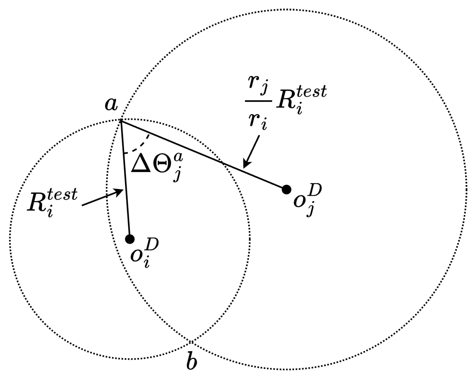
2.2.3. Finding Position Candidate by Circle Intersection

We utilize circle intersection to find the position candidate in the database with the same radius ratio, $R_j/R_i=r_j/r_i$, and the same angle difference, $\Delta {\mathsf{\Theta }}_j=\Delta {\theta }_j$. The coordinates of the intersections of two circles with known centers and radii can be calculated as described in [24]. We find the intersection of two circles centered at $o_i^D$ and $o_j^D$ with radii $R_i$ and ${\displaystyle \frac{r_j}{r_i}}{R}_i$, respectively. While the radius $R_i$ is unknown, the ratio of the radii of the two circles must be $r_i:r_j$. However, there exist infinitely possible values for $R_i$ where the circles can intersect. For each $R_i$, the polar coordinates $(R_i,{\mathsf{\Theta }}_i)$ and $(R_j,{\mathsf{\Theta }}_j)$ of the two database objects with respect to the circle intersection can be calculated. If the polar coordinates have the same relative angle, $\Delta {\mathsf{\Theta }}_j=\Delta {\theta }_j$, we take the intersection as the position candidate. Binary search is employed to efficiently iterate over possible candidate radii $R_i$. A graphical representation of the algorithm can be seen in Figure 7.

Algorithm 2 summarizes how to find the position candidate by circle intersection. The initial search range for $R_i$ is determined based on the following condition [24] to ensure that the two circles intersect at two points:

$$|R_i-R_j|<d<R_i+R_j$$

(4)

where d is the distance between the centers of the two circles. The algorithm calculates the intersections and checks whether the relative angle around each intersection is approximately the same as the relative angle of the image objects, $\Delta {\theta }_j$, within a pre-specified tolerance, ${\delta }_{\theta }$. If not, the search proceeds within one of the two halves. The decision to adjust $R_i^{test}$ upwards or downwards is based on the relative angles with respect to the current intersections.

2.3. Data Fusion with Inertial Measurements

From the perspective of data fusion, the sensor measurements of the map-based navigation system are generated by the map-matching block and the AHRS block, as depicted in Figure 1. The probabilistic data fusion block utilizes these subsystems’ outputs to provide navigational solutions, such as position, velocity, and attitude. More specifically, the horizontal position and velocity are estimated by the probabilistic data fusion block. The altitude is assumed to be obtained by other means, and the attitude from the AHRS block is bypassed. The data fusion block obtains position measurements from the map-matching block and acceleration measurements from the AHRS block.

The Kalman filter is employed here to provide estimates of position and velocity over time. The Kalman filter is a computationally efficient tool for obtaining a continuous stream of navigational solutions by fusing measurements at different rates. The Kalman filter equations are provided in Appendix A, which is detailed further in [25].

The Kalman filter operates through two main phases: prediction and update. The prediction stage uses the process model, given by Equation (A5), to predict the current state based on the state from the previous time step and the acceleration measurement. During the update phase, it adjusts the state estimate by utilizing the discrepancy between the actual and predicted measurements, as calculated by the measurement model in Equation (A11). Since the map-based navigation system is designed for use when the GNSS is unavailable, it uses the last known GNSS/INS outputs as the initial estimate of position and velocity. Every time acceleration data arrive, the prediction stage is executed. The position measurement from image processing and map matching is used in the update stage. The resulting state estimate of the Kalman filter comprises the primary navigational output of the map-based navigation system.

3. Flight Experiments

The proposed map-based navigation system is verified using real-time data from a multicopter drone in real-world environments.

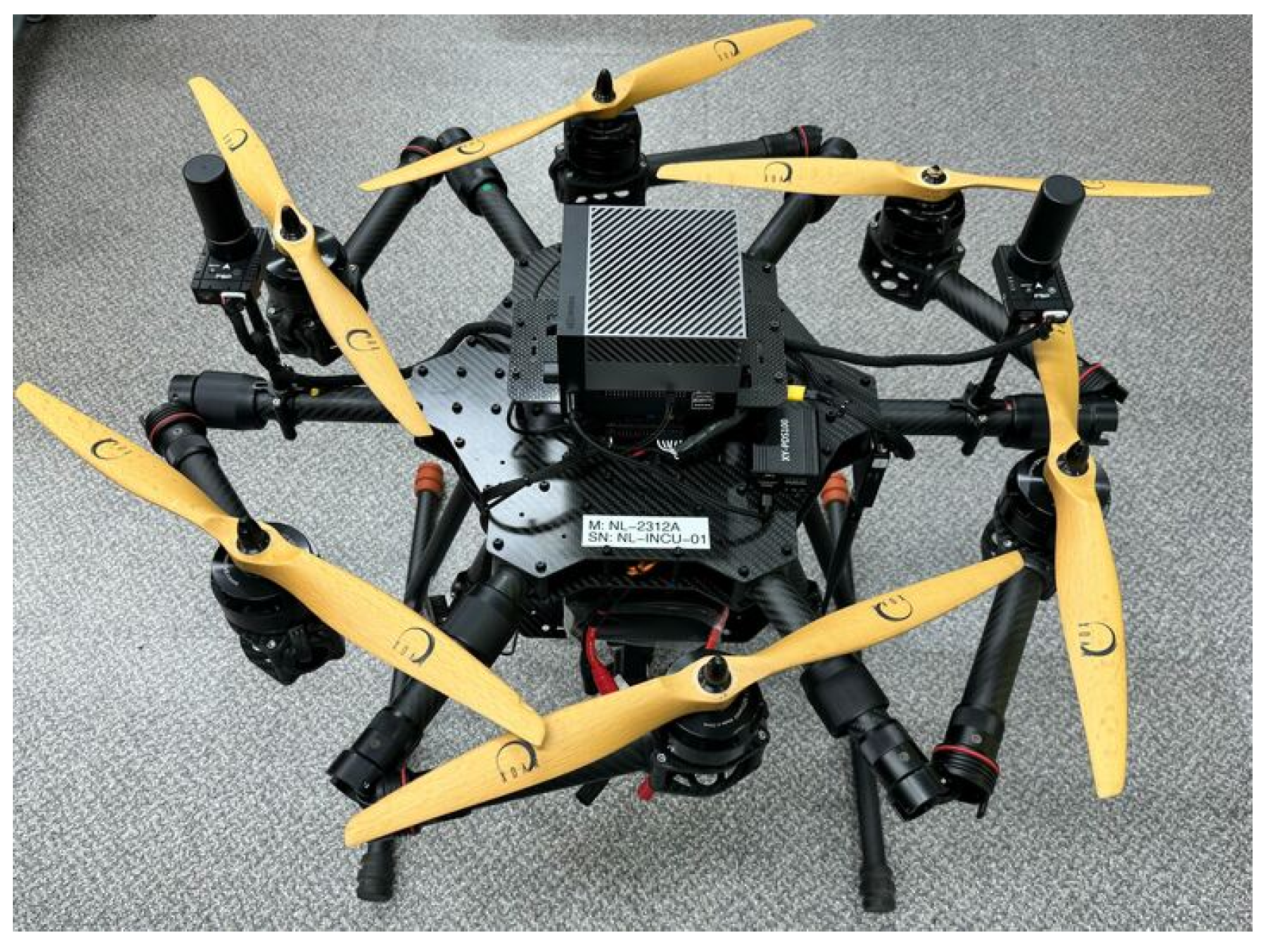
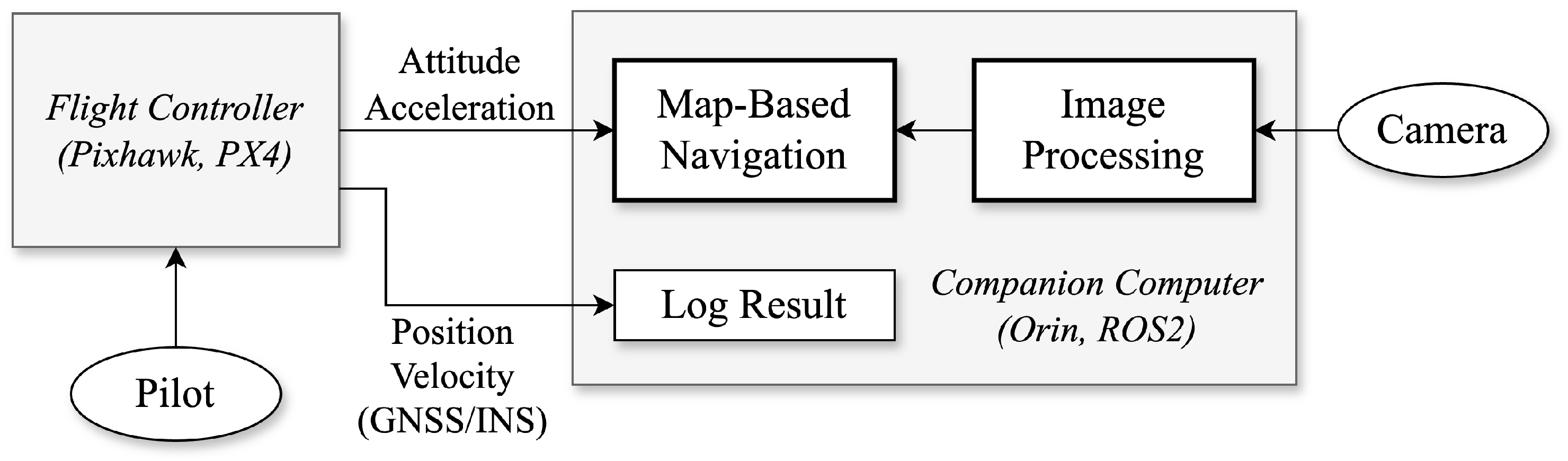
3.1. Unmanned Aircraft System

Figure 8 shows the multicopter drone used in the flight experiments. This is a hexacopter drone built with custom body frames. The drone is equipped with a gimbaled camera that is controlled to look downward during flight. An off-the-shelf flight controller, Pixhawk 6X, with the open-source PX4 Autopilot project, is responsible for the automatic control of the drone. The flight controller features a built-in GNSS receiver and IMUs. The AHRS outputs, i.e., attitude, are available from the flight controller. GNSS/INS solutions are used for flight control, while map-based navigation does not rely on GNSS/INS solutions. Real-time kinematics (RTK) GNSS is used as ground truth to assess the accuracy of the map-based navigation system.

The map-based navigation process, including image processing, map matching, and probabilistic data fusion, is conducted on a companion computer, specifically a Jetson AGX Orin Development Kit. The map-based navigation system software is implemented within a Robot Operating System 2 (ROS2) environment. The software architecture and the data flow of the companion computer are depicted in Figure 9.

3.2. Database Generation

The database is generated prior to the flight experiments. First, an unmanned aircraft equipped with RTK GNSS captures images of the entire test area. The acquired images are then aligned to create a complete map, from which buildings and greenhouses to be used for ground object recognition are masked. Masking methods include manual labeling and deep learning-based image segmentation. Subsequently, the latitude and longitude values of the center points of these masks are calculated and stored using the acquired masks and images. Figure 10 illustrates how the image of a test area is transformed into a map database in the form of a meta image. The map database is stored as a JSON file on the drone’s file system, which the map-matching algorithm can read.

3.3. Test Area and Scenario

The flight test was conducted in three different rural areas in Yangpyeong-gun, Gyeonggi-do, Republic of Korea, as illustrated in Figure 11, Figure 12 and Figure 13, which display an aerial view of each area along with the drone’s true and estimated trajectories. Altitudes ranged from 92 m to 132 m above ground level. These test environments were chosen for their diversity, ensuring sufficient visible objects.

Throughout the experiments, a pilot manually controlled the drone. Thus, the drone’s velocity was not necessarily constant during flights and varied from flight to flight. For example, in Area 1, the flight speed ranged between 2 and 7 m/s, while in Area 2, it was maintained between 4 and 6 m/s. This variability introduced randomness into the flight conditions, facilitating a more robust verification of the proposed system’s practicality.

The map-based navigation system was executed with the initial estimate of position and velocity from the GNSS/INS block, simulating scenarios where the GNSS is unavailable. The proposed navigation system recursively estimates position and velocity without using the GNSS. Concurrently, the RTK GNSS solutions were logged to serve as a reference for later assessing the accuracy of the map-based navigation outputs.

3.4. Results and Discussion

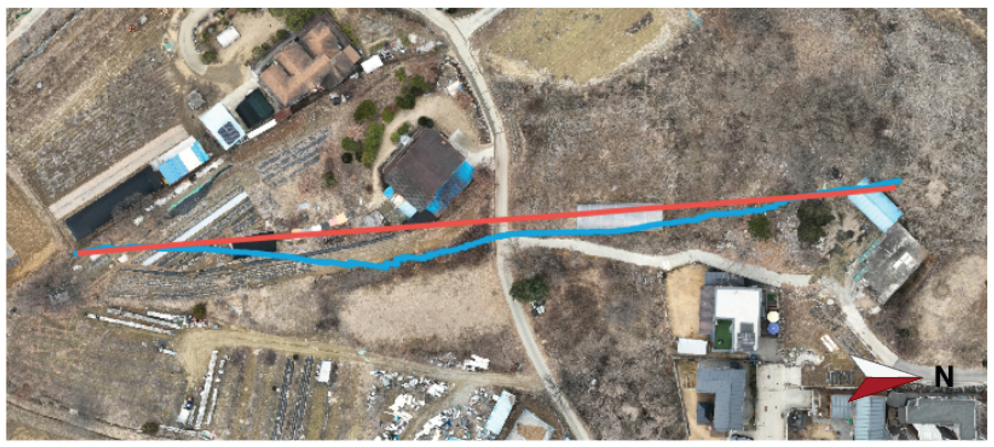
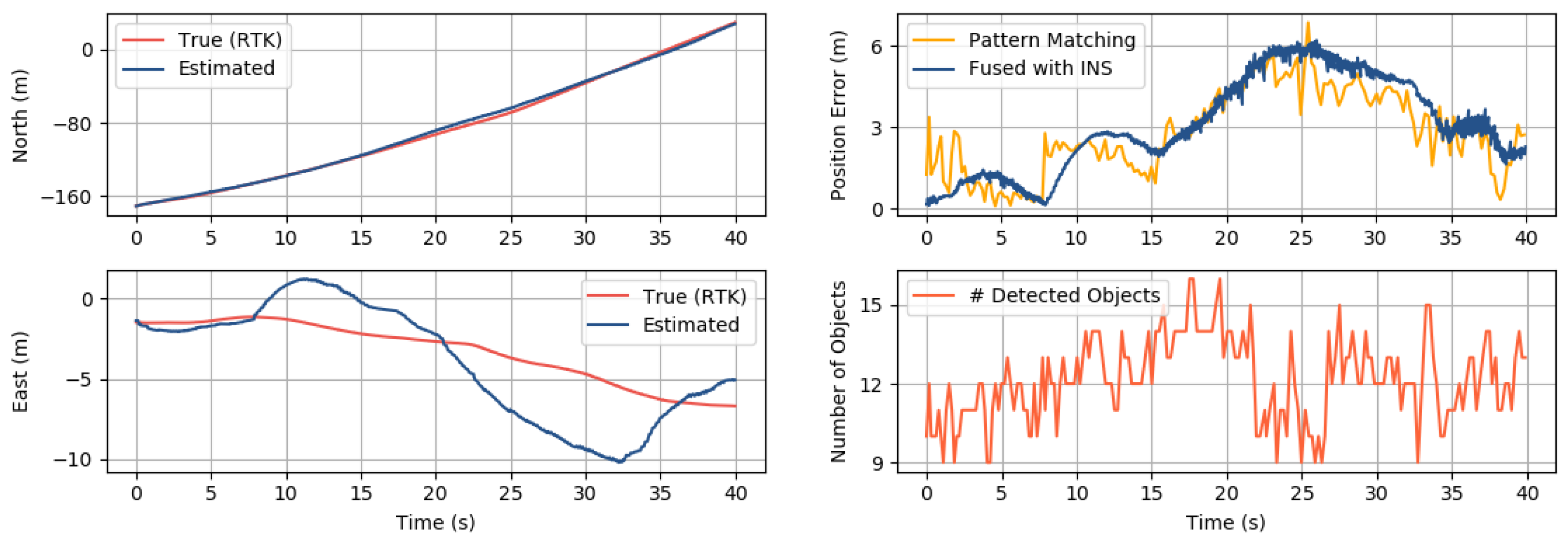
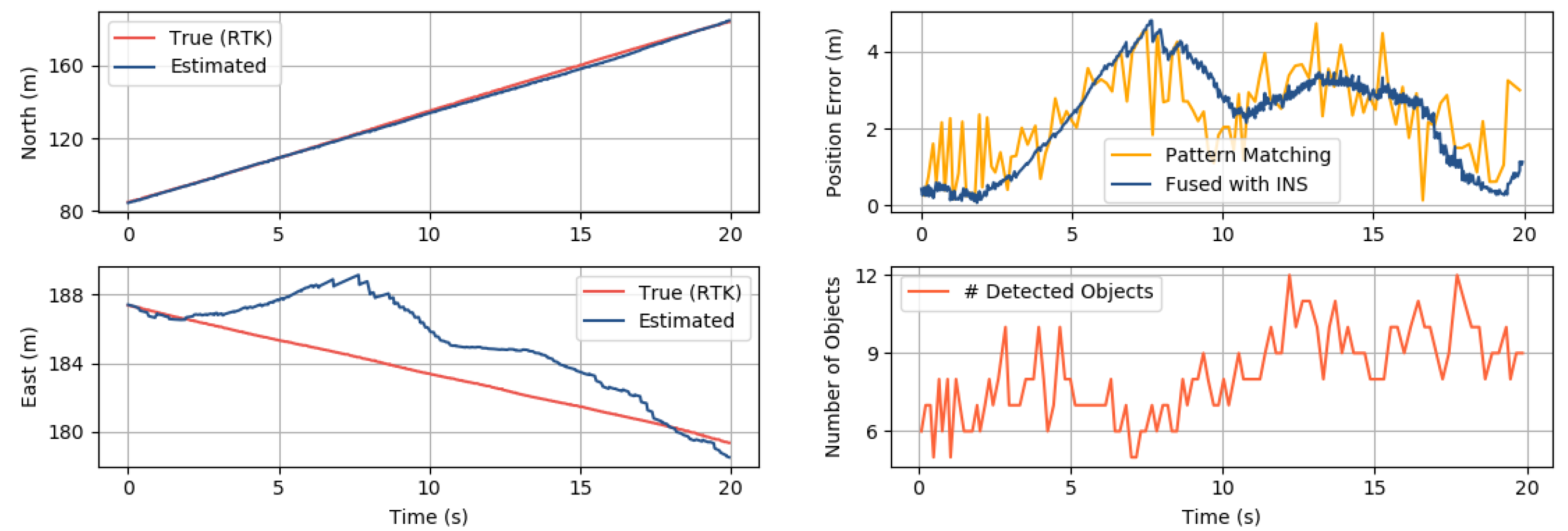
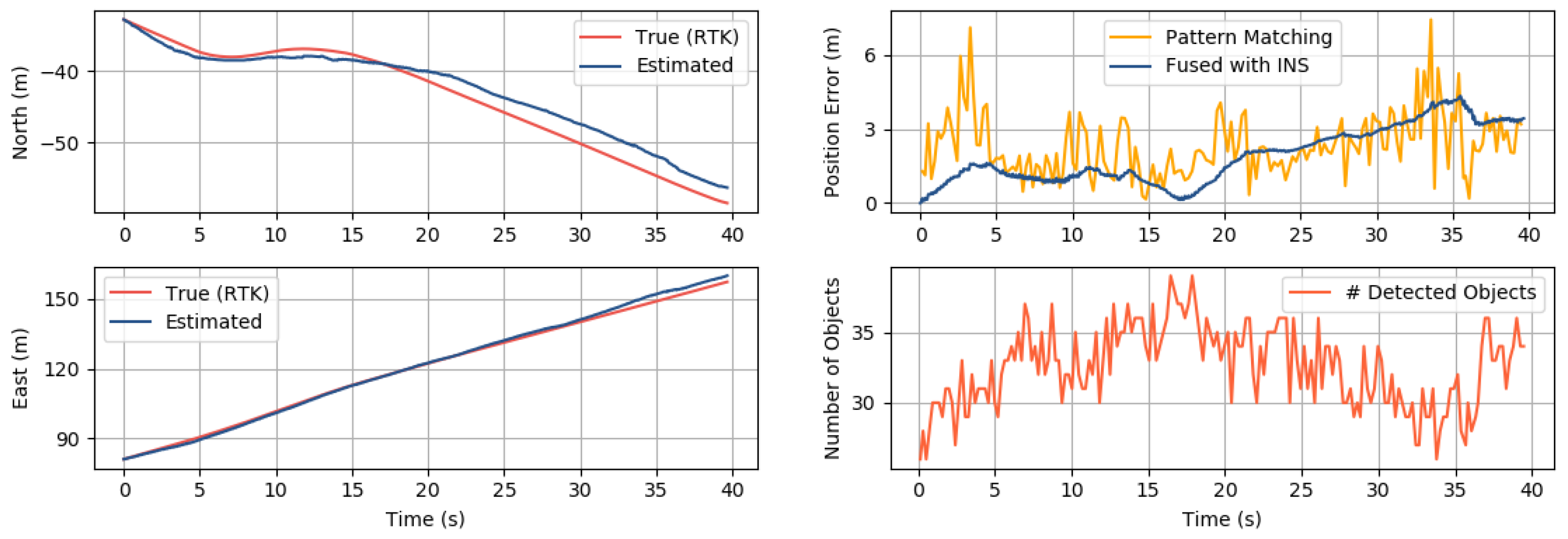
3.4.1. Position Accuracy

Figure 14, Figure 15 and Figure 16 show the position estimate results in Area 1-3, respectively. The horizontal position estimates are presented in meters along the north and east axes. These are compared with the RTK GNSS/INS output, which is considered the true position. The third subplot represents the horizontal distance error from the true position plotted over time. Although the raw estimates from the pattern matching were noisy, the fusion with the INS helped attenuate the noise from the image-based measurements.

Mathematically, the distance error $d_e$ is obtained as

$$d_e=\sqrt{n_e^2+e_e^2}$$

(5)

where $n_e$ and $e_e$ denote errors in the north and east positions, respectively. In order to evaluate the overall accuracy throughout the navigation, the root mean squared error (RMSE) is calculated as

$$\mathrm{RMSE}=\sqrt{{\displaystyle \frac{1}{N}}\sum _{k=1}^N{\left(d_e\left(k\right)\right)}^2}$$

(6)

where $d_e\left(k\right)$ is the k-th distance error and N is the total number of estimates. The RMSE values for the test areas are presented in

Table 3. Summary of characteristics and results of test cases.

Name	Height	Speed	# Objects	RMSE
Area 1	92 m	2–7 m/s	9–15	3.33 m
Area 2	132 m	4–6 m/s	5–12	2.60 m
Area 3	127 m	2–4 m/s	25–39	2.22 m

along with other characteristics of the test areas. The results demonstrate that the proposed map-based navigation system provides stable output, with at least about seven ground objects detected on the image under various conditions. Although not statistically significant, there was a tendency for increased velocity variation to result in larger errors. This issue is discussed further in Section 3.4.3.

3.4.2. Computation Time

The object detection model in the image-processing block generates five meta images every second. Meanwhile, the pattern-matching algorithm is configured to return the current best estimate every 50 ms. Consequently, the map-matching block provides position measurements at a frequency of 5 Hz to the data fusion block. As the state prediction phase of the Kalman filter is executed every time new acceleration data are available, the data fusion block outputs the navigation solution at 100 Hz.

3.4.3. Limitations

One can observe that the position estimate in Figure 14 oscillates slowly over time. The underlying cause can be traced to the velocity estimates presented in Figure 17. The velocity estimates overshoot the true value before eventually converging to it. The delayed velocity estimate is attributed to the map-based navigation relying heavily on position measurements without utilizing velocity measurements. Providing velocity measurements, i.e., optical flow, would increase the observability of velocity and help correct the INS drift more effectively. Relying more on acceleration measurements using better IMUs could also be a viable alternative.

Another limitation of this approach is that it cannot operate properly where the aerial image does not contain a sufficient number of objects that the deep learning model is trained to detect. Not all areas have detectable ground objects, and abrupt obstructions caused by clouds or fog may disable the vision-based navigation system. Additional object types could be incorporated to further improve the proposed navigation system. Incorporating more types of ground objects would benefit the system by increasing the number of objects, decreasing the ambiguity of pattern matching, and covering a broader range of geographical locations. For stable operation in various environments, it is necessary to continuously track environmental changes and further train the model for new environments.

Large objects like roads and agricultural fields can be detected. However, since only a part of the object is captured in the image, the center of the bounding box does not consistently represent the object’s location. These objects would be more usable if the image processing could locate each corner of the object, for example. This issue could be addressed by developing an image-processing algorithm tailored to our needs.

4. Conclusions

This paper introduced a map-based navigation system with a novel approach employing pattern matching of ground objects between the aerial image and the map database. In the matching process, each object is represented as a tuple containing its coordinates and label. The proposed map-based navigation system uses the Kalman filter to fuse the image-based localization result with the INS. The flight experiments demonstrated that the proposed method provided stable output over buildings and greenhouses in various conditions.

References

1. Kim, Y.; Hong, K.; Bang, H. Utilizing out-of-sequence measurement for ambiguous update in particle filtering. IEEE Trans. Aerosp. Electron. Syst. 2018, 54, 493–501. [Google Scholar] [CrossRef]
2. Spiegel, P.; Dambeck, J.; Holzapfel, F. Slant range analysis and inflight compensation of radar altimeter flight test data. Navig. J. Inst. Navig. 2016, 63, 491–507. [Google Scholar] [CrossRef]
3. Sim, D.G.; Park, R.H.; Kim, R.C.; Lee, S.U.; Kim, I.C. Integrated position estimation using aerial image sequences. IEEE Trans. Pattern Anal. Mach. Intell. 2002, 24, 1–18. [Google Scholar]
4. Rodriguez, J.J.; Aggarwal, J. Matching aerial images to 3-D terrain maps. IEEE Trans. Pattern Anal. Mach. Intell. 1990, 12, 1138–1149. [Google Scholar] [CrossRef]
5. Kim, Y.; Bang, H. Vision-based navigation for unmanned aircraft using ground feature points and terrain elevation data. Proc. Inst. Mech. Eng. Part J. Aerosp. Eng. 2018, 232, 1334–1346. [Google Scholar] [CrossRef]
6. El Garouani, A.; Alobeid, A.; El Garouani, S. Digital surface model based on aerial image stereo pairs for 3D building. Int. J. Sustain. Built Environ. 2014, 3, 119–126. [Google Scholar] [CrossRef]
7. Shan, M.; Wang, F.; Lin, F.; Gao, Z.; Tang, Y.Z.; Chen, B.M. Google map aided visual navigation for UAVs in GPS-denied environment. In Proceedings of the 2015 IEEE International Conference on Robotics and Biomimetics (ROBIO), Zhuhai, China, 6–9 December 2015; pp. 114–119. [Google Scholar]
8. Zhuo, X.; Koch, T.; Kurz, F.; Fraundorfer, F.; Reinartz, P. Automatic UAV image geo-registration by matching UAV images to georeferenced image data. Remote. Sens. 2017, 9, 376. [Google Scholar] [CrossRef]
9. Bay, B.; Andreas, E.; Tuytelaars, T.; Van Gool, L. Speeded-up robust features (SURF). Comput. Vis. Image Underst. 2008, 110, 346–359. [Google Scholar] [CrossRef]
10. Bublee, E.; Rabaud, V.; Konolige, K.; Bradski, G. ORB: An efficient alternative to SIFT or SURF. In Proceedings of the International Conference on Computer Vision, Barcelona, Spain, 6–13 November 2011. [Google Scholar]
11. Hong, K.; Kim, S.; Bang, H. Particle filter approach to vision-based navigation with aerial image segmentation. Aerosp. Inf. Syst. 2021, 18, 964–972. [Google Scholar] [CrossRef]
12. Wang, T.; Celik, K.; Somani, A.K. Characterization of mountain drainage patterns for GPS-denied UAS navigation augmentation. Mach. Vis. Appl. 2016, 27, 87–101. [Google Scholar] [CrossRef]
13. Volkova, A.; Gibbens, P.W. More robust features for adaptive visual navigation of UAVs in mixed environments. J. Intell. Robot. Syst. 2018, 90, 171–187. [Google Scholar] [CrossRef]
14. Kim, Y. Aerial map-based navigation using semantic segmentation and pattern matching. arXiv 2021, arXiv:2107.00689. [Google Scholar]
15. Park, J.; Kim, S.; Hong, K.; Bang, H. Visual semantic context and efficient map-based rotation-invariant estimation of position and heading. Navig. J. Inst. Navig. 2024, 71, 634. [Google Scholar] [CrossRef]
16. Girshick, R.; Donahue, J.; Darrell, T.; Malik, J. Rich feature hierarchies for accurate object detection and semantic segmentation. In Proceedings of the IEEE Conference on Computer Vision and Pattern Recognition, Columbus, OH, USA, 23–28 June 2014; pp. 580–587. [Google Scholar]
17. Girshick, R. Fast r-cnn. In Proceedings of the IEEE International Conference on Computer Vision, Santiago, Chile, 7–13 December 2015; pp. 1440–1448. [Google Scholar]
18. Ren, S.; He, K.; Girshick, R.; Sun, J. Faster R-CNN: Towards real-time object detection with region proposal networks. IEEE Trans. Pattern Anal. Mach. Intell. 2016, 39, 1137–1149. [Google Scholar] [CrossRef] [PubMed]
19. He, K.; Gkioxari, G.; Dollár, P.; Girshick, R. Mask r-cnn. In Proceedings of the IEEE International Conference on Computer Vision, Venice, Italy, 22–29 October 2017; pp. 2961–2969. [Google Scholar]
20. Liu, W.; Anguelov, D.; Erhan, D.; Szegedy, C.; Reed, S.; Fu, C.Y.; Berg, A.C. Ssd: Single shot multibox detector. In Proceedings of the Computer Vision—ECCV 2016: 14th European Conference, Amsterdam, The Netherlands, 11–14 October 2016; Proceedings, Part I 14. Springer: Cham, Switzwerland, 2016; pp. 21–37. [Google Scholar]
21. Wang, C.Y.; Bochkovskiy, A.; Liao, H.Y.M. YOLOv7: Trainable bag-of-freebies sets new state-of-the-art for real-time object detectors. In Proceedings of the IEEE/CVF Conference on Computer Vision and Pattern Recognition, Vancouver, BC, Canada, 17–24 June 2023; pp. 7464–7475. [Google Scholar]
22. Aihub Dataset. Available online: https://www.aihub.or.kr/ (accessed on 14 April 2024).
23. Fischler, M.A.; Bolles, R.C. Random sample consensus: A paradigm for model fitting with applications to image analysis and automated cartography. Commun. ACM 1981, 24, 381–395. [Google Scholar] [CrossRef]
24. Intersection of two circles. Available online: https://paulbourke.net/geometry/circlesphere/ (accessed on 20 March 2024).
25. Kim, Y.; Bang, H. Introduction to Kalman filter and its applications. In Introduction and Implementations of the Kalman Filter; Govaers, F., Ed.; IntechOpen: London, UK, 2018. [Google Scholar]
Figure 1. Block diagram of the proposed map-based navigation system.
Drones 08 00375 g001
Figure 2. The configuration of labeled ground objects is used to match the aerial image with the database. The red rectangles denote the result of object detection on the aerial image. The red cross denotes the center of the image. The black dots denote the labeled objects, which are an image representation of the meta image. The meta image is represented as a set of tuples in the map-based navigation system. Each tuple corresponds to a black dot and contains the object’s label and horizontal coordinates.
Drones 08 00375 g002
Figure 3. Example of training dataset (images and labels) for ground object recognition. (a) 25 cm/pixel, 512 × 512 ; (b) 25 cm/pixel, 1024 × 1024 ; (c) 12 cm/pixel, 512 × 512 .
Drones 08 00375 g003
Figure 4. Examples of instance segmentation in the validation dataset.
Drones 08 00375 g004
Figure 5. Exemplary results of image processing on aerial images. Green dots denote buildings, and blue dots denote greenhouses. The set of dots, also referred to as a meta image, is used in map matching.
Drones 08 00375 g005
Figure 6. The polar coordinates of the image objects with respect to the image center.
Drones 08 00375 g006
Figure 7. Graphical representation of circle intersection of Algorithm 2.
Drones 08 00375 g007
Figure 8. Multicopter drone used in the flight experiments.
Drones 08 00375 g008
Figure 9. Software architecture and the data flow of the companion computer and the flight controller.
Drones 08 00375 g009
Figure 10. Graphical representation of database generation of a test area. The aerial image (left) is converted to a meta image (right) offline. The map database in the form of a meta image is stored on the drone.
Drones 08 00375 g010
Figure 11. Drone trajectory (red: true; blue: estimated) on the aerial image of Area 1.
Drones 08 00375 g011
Figure 12. Drone trajectory (red: true; blue: estimated) on the aerial image of Area 2.
Drones 08 00375 g012
Figure 13. Drone trajectory (red: true; blue: estimated) on the aerial image of Area 3.
Drones 08 00375 g013
Figure 14. Position estimates over time compared with the RTK GNSS/INS estimates in Area 1. The position error denotes the horizontal distance error. The number of objects used in pattern matching is also shown.
Drones 08 00375 g014
Figure 15. Position estimates over time compared with the RTK GNSS/INS estimates in Area 2. The position error denotes the horizontal distance error. The number of objects used in pattern matching is also shown.
Drones 08 00375 g015
Figure 16. Position estimates over time compared with the RTK GNSS/INS estimates in Area 3. The position error denotes the horizontal distance error. The number of objects used in pattern matching is also shown.
Drones 08 00375 g016
Figure 17. Velocity estimates over time compared with the RTK GNSS/INS estimates in Area 1.
Drones 08 00375 g017