Abstract
Inspired by hummingbirds and certain insects, flapping wing micro aerial vehicles (FWMAVs) exhibit potential energy efficiency and maneuverability advantages. Among them, the bi-directional motor-driven tailless FWMAV with simple structure prevails in research, but it requires active pose control for hovering. In this paper, we employ deep reinforcement learning to train a low-level hovering strategy that directly maps the drone’s state to motor voltage outputs. To our knowledge, other FWMAVs in both reality and simulations still rely on classical proportional-derivative controllers for pose control. Our learning-based approach enhances strategy robustness through domain randomization, eliminating the need for manually fine-tuning gain parameters. The effectiveness of the strategy is validated in a high-fidelity simulation environment, showing that for an FWMAV with a wingspan of approximately 200 mm, the center of mass is maintained within a 20 mm radius during hovering. Furthermore, the strategy is utilized to demonstrate point-to-point flight, trajectory tracking, and controlled flight of multiple drones.
1. Introduction
Bees and certain other insects are capable of hovering, while hummingbirds are the only bird species capable of such sustained aerial behavior [1]. Mimicing the flight of these biological flyers, flapping wing micro aerial vehicles (FWMAVs) is an attractive solution for drones at the scale of centimeters or decimeters. At this scale, fixed wings struggle to maintain high speeds for sufficient lift, and rotor-based forward flight suffers from inadequate energy efficiency [2]. In contrast, flapping wing designs hold promise for maneuverability within confined spaces and greater energy efficiency [3,4]. However, as of now, due to manufacturing flaws, insufficient motor power density, limited control methods, and other reasons [5,6], FWMAVs still struggle to emulate their counterparts in nature.
In the past few decades, several research teams have achieved liftoff and to some extent controlled flight of FWMAVs. Typically, researchers utilize crank-rocker mechanisms to convert the unidirectional rotation output of motors into flapping motion of wings, as demonstrated in projects such as Delfly and KUBeetle [7,8,9]. One limitation of this type of aircraft is its inability to alter the flapping amplitude of wings, only being able to adjust the flapping frequency, necessitating additional servo mechanisms to generate control torque. Other researchers have employed high-frequency input power modulation, driving wing flapping directly through piezoelectric or bidirectional motor rotation, as seen in projects like Robobee and Purdue hummingbird robot [10,11,12]. This approach allows for easy manipulation of wing kinematics, controlling the left and right flapping angles of wings independently, thus generating control torque through instantaneous wing kinematics modulation [13], without the need for additional mechanisms for control assistance.
The flight control of FWMAVs presents significant challenges, including complex system dynamics, severe underactuation, and limited control authority, among others [2,14]. Some researchers address these issues using classical feedback controllers. Karásek et al. employ a biologically inspired Proportional-Derivative (PD) controller for pitch and roll control of the Delfly Nimble, and a proportional and feedforward controller for yaw control [7]. Phan et al. use a PD controller for feedback control of the KUBeetle’s angular velocity, with three servos used to minimize the error between the desired and measured bodyrates [15]. These fixed-gain feedback architecture heavily relies on empirical engineering practices, involving trial and error for gain parameter tuning in both simulation and real-world scenarios [2,15]. As for FWMAVs without crank-rocker, Chirarattananon et al. propose a linear controller by sequentially adjusting parameters to accomplish increasingly complex control tasks [16]. Zhang et al. design a nonlinear geometric controller that theoretically ensures it is almost globally exponentially attractive and achieves attitude stabilization control during the liftoff process [14].
Researchers also attempt flight control of FWMAVs through learning-based methods. Chirarattananon et al. propose an iterative learning control algorithm, building upon the Robobee platform, to achieve imitation of insect-like landing on vertical walls with the aid of magnetic adhesion [17]. Fei et al. employ a hybrid strategy, combining adaptive robust control with the Deep Deterministic Policy Gradient (DDPG) algorithm, to enable FWMAVs to execute aggressive maneuvers like 180-degree yaw turns and 360-degree body rolls [18,19]. Nozawa et al. utilize the Deep Q-Network algorithm to control the pitch angle of a FWMAV [20], yet this control is discretized, capable only of maintaining the pitch angle within a certain range. In fact, the aforementioned studies only use learning-based methods to perform some specific tasks, while relying on classical feedback controllers to achieve pose control tasks such as hovering.
The control issues of FWMAVs may benefit from insights gained through training quadcopter flight using learning-based method. While many studies focus on high-level decision-making [21,22], particularly trajectory planning, there are still some works utilizing learning-based methods to perform low-level control. These works directly output motor voltage commands for pose control, thereby eliminating the need for an additional classical lower-level pose controller. Koch et al. propose a quadrotor low-level controller based on reinforcement learning which can track the set values of angular velocity [23]. Molchanov et al. train a stable low-level quadrotor controller that can drive the Z-axis of the drone’s body coordinates vertically upward and minimize position and velocity errors from randomly sampled initial conditions within a certain range in a short time [24].
In this paper, we choose a hummingbird-like bi-directional motor-driven tailless FMWAV as the subject due to its simplicity, compactness, and potential maneuverability. The goal is to develop a hover flight strategy capable of consistently maintaining the center of mass of the FWMAV’s torso within a 50 mm diameter space during flight. Considering the wingspan of this kind of FWMAV is about 200 mm, this positional error is acceptable. The experiments are performed in a high-fidelity simulation environment, which has complete system dynamics, including motor-driven wing dynamics and flapping flight aerodynamics. We use reinforcement learning to train the hover strategy. The training is conducted in 20 parallel environments, employing the widely-used Proximal Policy Optimization (PPO) algorithm to ensure stability in policy updates. Reasonable state and action spaces are selected, with particular emphasis placed on utilizing a sliding window of historical states and actions to expand the state space, addressing asynchronous control issues [25]. Boundary conditions and reward functions are designed through understanding of the problem and iterative refinement. The final strategy is obtained through two training sessions, each consisting of 50 million steps, with different boundary conditions set for each training session. During the first training session, with larger boundary values, the FWMAV primarily learns to maintain attitude stability. In the second training session, boundary values are reduced to enhance the precision of the position control.
Eventually, the trained policy can enable the FWMAV to hover at any set point in space and additionally perform vertical, forward, and lateral flights, enabling point-to-point flight from the initial position to distant target points. This policy effectively serves as a low-level pose controller, while avoiding manual tuning of complex gain parameters. To our knowledge, other FWMAVs in reality or simulation still rely on pose controllers similar to traditional cascaded PD. As a demonstration of the policy’s versatility, trajectory tracking along a circular path and the control of multiple drones are shown within the simulation.
The structure of this paper is as follows: Section 2 elaborates on the modeling of FWMAVs and briefly introduces reinforcement learning method. Section 3 provides a detailed description of the experimental intricacies of reinforcement learning training, alongside the measurement of forces on the FWMAV in simulation. Section 4 presents a analysis of training results, supplemented with demonstrations of several applications. Finally, Section 5 concludes and points out future research directions.
2. Models and Methods
In this chapter, the fundamental model of our FWMAV is established, encompassing the mechanical structure, wing actuation model, and aerodynamics. Subsequently, we analyze the generation of control forces and torques, then outline the control challenges of this type of drone. Finally, the reinforcement learning algorithm used for continuous action control in this paper is briefly introduced.
2.1. Drone Model and Flapping Mechanisms
The bi-directional motor driven tailless FWMAV prototype implemented in our lab is shown in Figure 1a. Corresponding SolidWorks model is shown in Figure 1b, where a hollow carbon fiber frame is employed as the torso and two rigid thin sheets as the wings. Note that the torso is vertical here, an orientation resembling that of a hummingbird during flight, where it typically maintains a slight angle with the vertical direction, as opposed to large-scale flapping-wing aerial vehicles or fixed-wing aerial vehicles.
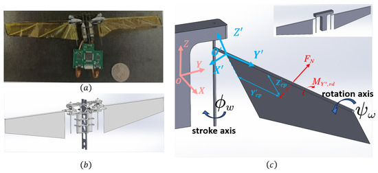
Figure 1.
Our FWMAV. (a) FWMAV in reality. (b) SolidWorks model. (c) Unified Robot Description Format(URDF) model, with reference coordinate systems.
Two brushless direct current motors are employed to drive the wings separately, enabling a symmetric flapping motion between the upstroke and downstroke phases through gearsets and torsion springs. In addition, the wings undergo passive rotation about the rotation axis due to forced vibration. Elastic components can function as energy storage elements to preserve the kinetic energy, and a properly configured flapping frequency can induce mechanical resonance, leading to a significant enhancement in the energy efficiency of the entire system [12,26]. In an ideal situation, the kinetic and potential energies of the mechanical components within the system can be conserved, with the majority of the motors’ work dedicating to overcoming system damping forces and aerodynamic drag on the wings, without being utilized to counteract the inertia force resulting from the high-frequency reciprocating motion of the wings [27].
To reduce the complexity in simulation, the Unified Robot Description Format(URDF) model is simplified into five components: torso, two rods, and two wings, as shown in Figure 1c. The mass and rotational inertia are systematically identified in reality and then injected into the urdf file. The body coordinate system OXYZ is fixed on the torso. The coordinate system is at the right wing root. The axis points radially outward, and the axis points opposite to the chordwise direction of the wing.
The wing can rotate around the rotation axis, with the rotation angle denoted as . The T-shaped rod, swinging together with the wing up and down around the stroke axis, is referred to as the stroke motion, where the stroke angle is denoted as . The wing actuation model can be expressed as follows [27]:
where u signifies the input voltage, is the lumped input gain, denotes the total moment of inertia, and stand for the combined linear and aerodynamic damping coefficients respectively, represents the torsional spring coefficient.
Calculating aerodynamic forces for FWAMVs typically assumes that these forces are computed under quasi-steady aerodynamic conditions [28]. Transient aerodynamic phenomena such as delayed stall, rotational circulation, and wake capture [29] in low Reynolds number flight scenarios are indirectly expressed through the aerodynamic coefficient , where denotes the angle of attack of the wing.
To ensure clarity in the following aerodynamic discussions, we adopt Ellington’s proposed insect wing parameters [30] to model the wing, as illustrated in Figure 2. In this model, r is the radial distance, denotes the chord length, R is the wing span, and S stands for the wing area. The mean chord length is calculated as . Physical quantities with a hat ^ are dimensionless, such as represents the dimensionless radial distance of the k-th order central moment: , where .

Figure 2.
The parameterized wing model and the actual wing.
The aerodynamic forces are calculated using Blade Element Theory (BET). Considering a small chordwise strip of the wing located at a distance r from the wing root with an area , the relative airflow velocity is . For hovering or low-speed flight, the velocity of the torso is relatively small and can be neglected. Dynamic air pressure is . From the general form of aerodynamic force , the differential form and integral form with dimensionless parameters can be expressed as follows:
In the simulation, only the normal force on the wing surface is considered because it far exceeds the shear viscous forces acting parallel to the wing [29]. We have:
where the empirical formula for can be found in [28]. By applying the spatial resultant moment theorem, the point of application of force on the wing surface can be determined, namely and . and are the moments of the aerodynamic force in the normal direction of the wing surface about the Y-axis and Z-axis, respectively. They can both be calculated using the aforementioned BET approach [28]:
where the denotes the chordwise aerodynamic center coefficient [31].
As previously mentioned, while the motor actively drives the wing to perform the stroke motion, the wing undergoes passive rotation. This effect is described using rotational aerodynamic damping [28]:
2.2. Generation of Control Force and Torque
In flight control systems, the concept of averaging theory is widely applied [10,11], allowing the approximation of time-varying systems through their averaged values, provided there is sufficient separation of time constants [32]. In FWMAVs, as long as the flapping frequency f is sufficiently high, an averaged system can be used through a cycle-averaged froce coefficient [29]. Specifically, if the amplitude of the stroke angle is , the average lift of a single wing can be represented as:
where the detailed averaging analysis with time scale separation can be found in [13].
According to the wing kinematics modulation technique introduced by [13,33], below we demonstrate how our twin-motor driven tailless FWMAV generates lift and control torque solely through storke kinematic variations of its wings.
First, let the nominal amplitude be denoted as , corresponding to lift . Let the variation in amplitude be , as shown in Figure 3a, then the variation in lift is:
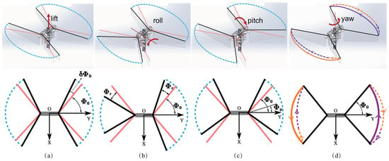
Figure 3.
Generation of lift and control torque through kinematic modulations of wings: (a) lift, (b) roll, (c) pitch. (d) yaw. (Pictures in the row below are depicted in top view. Pink and black lines denote the extreme stroke wing position before and after modulation, and blue dashed lines denote wingtip trajectory after modulation. In (d), orange and purple line denote wingtip trajectory during the first 0.5 T and the latter 0.5 T, and solid trajectories indicate faster average stroke angular velocities compared to dashed ones.)
Second, as shown in Figure 3b, induce a difference in amplitude between the left and right wings to generate the roll torque:
Third, altering the center surface of the stroke motion by an angle to generate pitch torque, as shown in Figure 3c, considering that is quite small, yeilds:
Last, utilizing the split cycle parameter to generate the angular velocity difference between left and right wings, thereby generating yaw torque, as shown in Figure 3d. Here, we calculate during the downstroke (with the upstroke following a similar process). According to the process of calculating in Equation (4) and the synthesis of spatial moment vectors, after numerical approximation, the following holds:
Through the aforementioned analysis, it is evident that Sinusoidal voltage signals are applied to the left and right motors to achieve these wing kinematics variations through four control parameters, , , , and , corresponding to , , , and above. In addition, let , where is the voltage amplitude which generates sufficient lift force to counter the gravity. The wing flapping angle exhibit a quasi-sinusoidal waveform lagging behind the voltage signal, and these two sets of parameters are roughly proportional according to the analysis in [27]:
where . Specifically, the left and right motor input signals and at time t within one period T can be expressed as follows:
As the bi-directional motor driven FWMAV relies solely on two motors to fully control the six degrees of freedom, it suffers from severe underactuation. Additionally, due to the high sensitivity of this type of FWMAV, even minor adjustments in wing kinematics can result in significant changes in lift and torque outputs [11], posing a considerable challenge to its control.
2.3. Reinforcement Learning
Note that the symbols in the following discussion may conflict with those used earlier, but should not cause confusion in context. See the notation section at the end for details.
Reinforcement learning has increasingly been applied to address control problems in robotics, including aerial vehicles. In typical reinforcement learning setups, an agent continually interacts with the environment: it observes the current state , takes action according to its policy , receives a reward from the environment, and transitions to the next state. Through these repeated iterations, the agent learns about the task and refines its policy accordingly, as shown in Figure 4a. The yellow line represents the learning process in one step. Define the return as the weighted sum of rewards over time:
where is a discount factor between 0 and 1, used to balance the importance of current and future rewards. A closer to 1 emphasizes long-term rewards, but setting it too close to 1 can hinder training performance. The key mechanism of reinforcement learning is to find a policy which can execute optimal actions to maximize the return [34].

Figure 4.
Reinforcement learning framework. (a) General concept. (b) Actor-Critic algorithm.
At time t, the return is a random variable, but the agent needs to predict the value of , estimating the quality of future rewards to update the policy. At this point, taking the expectation of can eliminate its randomness. Define the action-value function as the expectation of with respect to under the condition of observing . The depends on and but does not depend on the states and actions at time t + 1 and beyond. Mathematically, it is expressed as: . can be used to measure the quality of taking action in state throughout the entire training episode when using policy .
Define the state-value function as the expectation of the action-value function with respect to the action variable at the current time t: . In policy learning, the objective function is defined as:
where represents the parameters of the policy . The goal is to maximize .
One common approach to policy optimization in reinforcement learning is the Actor-Critic method [35]. In this method, the Critic module approximates using the value network q with parameters , which it provides to the Actor to improve the policy, as illustrated in Figure 4b. Then can be approximated as according to the policy gradient theorem. Define the loss function of the value network using temporal-difference method:
All gradients can be obtained through backpropagation in the neural network, updating the parameters of the value network with gradient descent and the parameters of the policy network with gradient ascent becomes straightforward:
where are the learning rates. The final result is the policy after optimization.
In this paper, the Proximal Policy Optimization (PPO) algorithm [36], a member of the Actor-Critic algorithm family, is utilized for training. Unlike the original Actor-Critic algorithm, its Value Net directly estimates . To reduce the variance of policy gradient estimates and improve learning efficiency, the advantage function is computed using Generalized Advantage Estimation(GAE) method [37] within a given length-T trajectory segment:
In PPO, the trust region approach is used to approximate the objective function of the Policy Net, and a clipping technique is typically employed to ensure that the disparity between new and old parameters remains within acceptable bounds. Relevant papers usually use instead of in their notation [36], which can specifically be expressed as:
where .
3. Experiments
Based on the aforementioned physical model, a simulation environment is constructed by using the PyBullet physics engine [38]. The details of the system identification will be provided in another concurrently conducted work. This simulation is fully compatible with the OpenAI Gym environment. It can run independently on each CPU core, enabling parallel training to expedite sample collection efficiency and enhance training speed. The physics engine update frequency is set to 24 kHz, while the control step frequency is set to 1.2 kHz based on the performance of microcontrollers in reality. The steps used in reinforcement learning experiments are the control steps mentioned here. All experiments in this paper are conducted on a personal computer equipped with an i7-13790F processor and running Ubuntu 20.04.
In the context of the hovering for FWMAV, two prerequisites are paramount. Firstly, the FWMAV must be capable of generating adequate lift and three-axis torque. Secondly, it necessitates the implementation of a pose controller. In the following sections of this chapter, we discuss the relationship between the FWMAV voltage signal input and the force and torque output. Additionally, we detail the training of a pose controller using reinforcement learning.
3.1. Force and Torque
In this section, we measure the forces and torques experienced by the entire FWMAV during the flapping wing process, in preparation for subsequent reinforcement learning experiments. Additionally, an approximate linear relationship is verified between the relative control inputs , , , and , , , .
We fix the torso of the drone and measure the forces acting on the object attached to it, through which the forces exerted on the FWMAV can be inferred, akin to using force sensors in reality. Specifically, the voltages of the motors on the left and right sides are given as and . This corresponds to setting V and zeroing the four control inputs specified in Equations (12) and (13). All measurements start from the FWMAV’s static state. The data for the first few wing strokes represent the transient transition state, as shown in Figure 5. Only the voltage signal and wing motion for the one side is plotted. Both the force and torque undergo median filtering with a kernel size of 3.
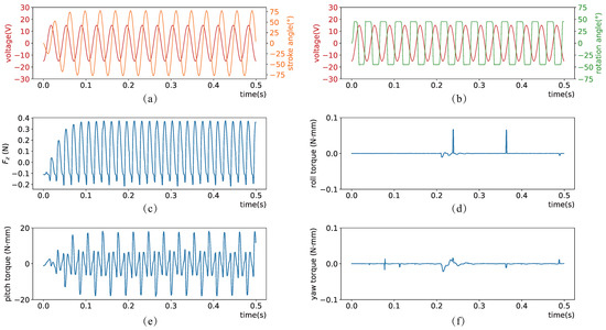
Figure 5.
Sinusoidal voltage input for 0.5 s with measured wing kinematics and body force/torques over time. (a) Single-sided voltage signal and wing stroke angle. (b) Single-sided voltage signal and wing rotation angle. (c–f) represent the overall resultant force in the vertical direction, as well as the overall roll torque, pitch torque, and yaw torque, respectively.
As shown in Figure 5a,b, though the wing stroke angle and the wing rotation angle both lag behind the voltage signal, the phase lag of the wing rotation angle is larger. In Figure 5c, the FWMAV is only subjected to the force of gravity initially, resulting in a force of approximately N in the Z-axis direction. As the wings start flapping, lift force is generated. At times, negative lift occurring, this phenomenon is consistent with the findings of Dickinson [29], who attribute it to the lagging rotational motion of the wings behind the stroke motion. While in subsequent reinforcement learning experiments, asymmetric mass properties are introduced to better simulate real-world imperfections in manufacturing and assembly, the URDF mass file is configured symmetrically here for clarity. Nonetheless, some noise still persists here due to computational errors. It’s noticeable that in the absence of control, the pitch torque significantly surpasses the roll and yaw torques, as shown in Figure 5d–f. This warrants particular consideration when crafting reinforcement learning reward functions later on.
Subsequently, the mean force and torque exerted on the FWMAV during a certain time are measured with variations of control inputs. Adopting a similar force measurement method as the previous experiment and following the averaging theory, we record the data between 1 s and 5 s and plot mean values as small dots in Figure 6. In each experiment, only one of the four control inputs, , , , , is varied. The thin red line represents the linear regression model using the least squares method. From the first row of Figure 6, it can be observed that , , , and exhibit proportional relationships with , , , and , aligning with the theoretical models in Equations (7)–(11). The second row of Figure 6 illustrates how , , and vary with . Notably, changes in have minimal impact on roll torque, while pitch torque and yaw torque demonstrate linear growth with , consistent with Equation (8) (without ) and Equations (9) and (10) (with ), respectively.
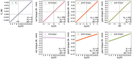
Figure 6.
Variation of mean force and torque on the FWMAV with control inputs.
Through the above analysis, it is evident that pitch torque is not solely controlled by , and yaw torque is also not solely controlled by . Both of them are influenced by , which means the four control inputs is not decoupled. This needs to be considered in the subsequent design of the reward function. Additionally, it is observed that when is set to its maximum value within the operational range, 15 V, the corresponding vertical upward force is approximately N. For our FWMAV, the gravitational force is N, so the maximum upward acceleration is equivalent to one gravitational acceleration. Admittedly, its control authority is rather small compared to quadrotors capable of generating vertical upward accelerations exceeding three gravitational accelerations [39].
3.2. Action and State Space
In the forthcoming sections, a pose controller is developed through reinforcement learning. The discussion delve into the specifics of action and state space selection, as well as providing a description of the formulation of boundaries, rewards, and training process. In our reinforcement learning experiments, the action is defined as the normalized . The state, constructed using , employs a sliding window of historical observations and actions with a window size of 40 steps to address system delays and asynchronous control issues [25]. Here, represents the error between the current position and the target position in world frame. In addition, represents the current rotation matrices. and denote the drone’s linear velocity and angular velocity in the body frame, respectively.
Domain randomization is adopted to enhance the robustness of the strategy and facilitate its transfer to real drones in the future. Specifically, the drone is initially placed along the Z-axis, and its altitude varies randomly between 400 mm and 600 mm, while the hover target position is always (0 mm, 0 mm, 500 mm). The Euler angles are initially set to 0 degrees, varying randomly within degrees, with the goal of maintaining them near 0. Note that the Euler angles follow the XYZ fixed angles convention as defined in the URDF standard. Additionally, the mass properties corresponding to different wing geometries are analyzed to generate a multivariate regression function. During training, each wing’s span varies randomly within mm from a base of 90 mm and URDF file is accordingly updated, with the wing’s mass and moments of inertia automatically generated by the regression function.
3.3. Boundary and Reward
The final strategy is obtained through two sessions of training, each with different boundary conditions and reward. In the first training session, the boundaries are set as follows:
During a training episode, the drone undergoes a reset each time it exceeds this boundary, initiating a new episode. In addition, the time boundary is set as s, meaning that a maximum of 18,000 control steps can be executed in one episode.
The reward function is designed to guide policy updates. Specifically, the policy, based on the previous step’s state , applies the action , and then the simulation computes the forward dynamics. Next, the environment calculates the reward using the reward function. The policy is updated based on the sequence of states, actions, and rewards. The reward function is defined as follows:
where the term is initially set to 25 and increases by 5 when the drone approaches within 25 mm of the hover target point. The coefficients represent penalties for position error, attitude, linear velocity, and angular velocity, respectively, and are set as follows: , , , and . All physical quantities define in above section and can be calculated during training from the data in the state space.
Note that the linear velocity penalty term only involves . While the hovering strategy appears to require minimizing and , experimental processes indicate that directly penalizing these velocities in the reward function is ineffective. Theoretically, an ideal hovering strategy would also produce inherent oscillations in the pitch direction due to the wings’ downstroke and upstroke, which generate certain . To address this, a coefficient is introduced and ultimately the trained strategy can maintain and within reasonable bounds.
The strategy trained from the first training session accomplishes hovering but exhibits notable position drift. Therefore, a second training session is carried out using the best model from the first session, along with modified boundary conditions and reward function. While other boundaries remain unchanged, position boundaries are narrowed as follows to improve precision:
and the initial value of in the reward function is adjusted to 50, with adjusted to 1600. It should be noted that without the first training session, starting from scratch with the modified conditions and parameters typically results in failure.
3.4. Training
Figure 7 illustrates the details of our parallel training framework. A separate simulation is established on each CPU core, with 20 parallel simulations used during training to enhance data collection efficiency. The sequence in the upper right corner, is generated as follows: In each simulation environment, the state is constructed using the initial observation, with historical observations and actions initially set to zero. Then, the initial Policy Net generates a Gaussian distribution for the action based on , from which the action is sampled. After applying to the FWMAV in the simulation environment, the reward is calculated according to the reward function. Next, state is constructed, and action is sampled from the distribution predicted by the Policy Net. After forward dynamics computation, the reward is obtained using the reward function. This process repeats until the sequences collected from all parallel environments reach the Rollout buffer’s size, at which point the Policy Net is updated. The black dashed box on the left contains the neural networks used in the PPO algorithm. The algorithm is implemented using the Stable-Baselines3 reinforcement learning library [40]. Both the Policy Net and Value Net are configured as neural networks with two hidden layers, each with 64 units.
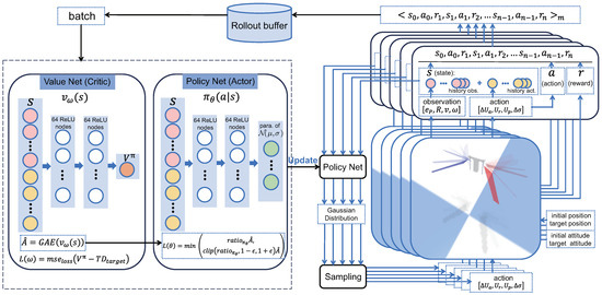
Figure 7.
Parallel training framework.
In the first training session, the batch size for updating the neural network is set to 256, and the discount factor, i.e., in Equation (14), is set to 0.99. In the second training session, the batch size is increased to 512, and is increased to 0.995 to more thoroughly consider the expectation of future rewards. In each training session, five independent episodes are evaluated every 20,000 steps, resulting in the episode reward versus training steps curve shown as the light blue line in Figure 8. The dark blue line represents a moving average calculated every 10 data points. Subfigure (a) represents the first training session, and subfigure (b) represents the second training session.
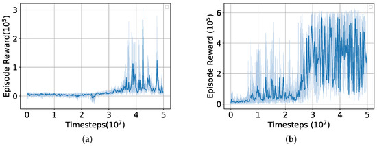
Figure 8.
Episode reward over timesteps. (a) first session, (b) second session.
3.5. Algorithm Comparison
To verify that the training results are not coincidental, we perform another training session from scratch using PPO with the same parameters as those used in the first session above. The reward curve obtained is shown in Figure 9. The algorithm is able to complete the hovering task, but the accuracy and response speed are certainly inferior to the policy optimized through the second session. Additionally, we train using the algorithms A2C [41] and DDPG [42], with all parameters kept the same except for the internal parameters of the algorithms. As shown in Figure 9, both algorithms fail to achieve high rewards.
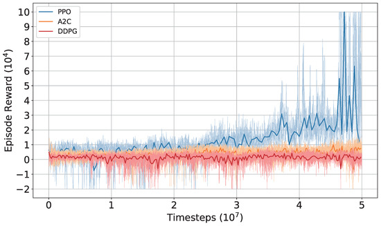
Figure 9.
Comparison of reward curves for three algorithms.
4. Results
The trained policy successfully achieves the goal of hovering within a 50 mm diameter range around the initial center of mass. It is noteworthy that, although the initial and target positions are close during training, the strategy demonstrates the capability to generalize to more distant targets. The strategy enables the FWMAV to hover at any set point in world frame and perform vertical, forward and lateral flights, enabling point-to-point flight from the initial position to distant target points, which serves effectively as a low-level pose controller. As a demonstration of its versatility, we showcase trajectory tracking along a circular path and the control of multiple drones within the simulation environment.
4.1. Open-Loop Flight
As a comparison, we present open-loop flight segments where the four control inputs are set to 0, and is set to constant values. Figure 10a shows the trajectories of the FWMAV starting from (0 mm, 0 mm, 1000 mm) for 0.8 s under different values. The trajectory with V is shown in red, and the trajectory with V is shown in blue. Figure 10b compares the positions and attitudes under the two values. It can be seen that the drone becomes unstable in a short period of time in both cases. Additionally, although V demonstrates a positive force along the z-axis in the force measurement experiment, as shown in the first subplot of Figure 6, this is not sufficient to lift the drone due to pitch oscillations.
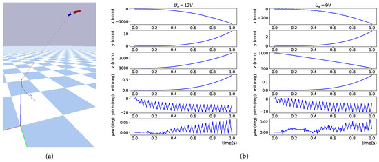
Figure 10.
Open-loop flight of the FWMAV: (a) trajectories (b) position and attitude within 1 s.
4.2. Hovering
The trained policy is applied to control the FWMAV for setpoint hovering. As shown in Figure 11a, after 2 s of adjustment, the position error between the torso’s center of mass and the set point does not exceed 10 mm within the third second. Figure 11b illustrates the position and attitude of the FWMAV hovering within 20 s. Note that the FWMAV exhibits inherent oscillations in the pitch direction due to wing flapping, leading to position fluctuations in the x direction. Since the state space during training observed the error between the current position and the target position, our policy can achieve hovering at any arbitrary point in space. By performing a coordinate transformation before inputting the state into the policy, the FWMAV can hover with different yaw angles. These two points are demonstrated in the experimental results of the following sections.
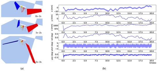
Figure 11.
Hovering at (0 mm, 0 mm, 1000 mm). (a) The trajectory of the first three seconds. The red thin line denotes the trajectory of the torso’s center of mass, while the yellow small ball has a radius of 5 mm centered on the target point. (b) Position and attitude within 20 s.
4.3. Point to Point Flight
The trained policy enables the drone to fly to set points farther than those encountered during training and maintain hovering at these positions. Figure 12a demonstrates the FWMAV lifting off from (0 mm, 0 mm, 500 mm) and hovering at (0 mm, 0 mm, 1000 mm). Figure 12b illustrates the FWMAV flying forward from (0 mm, 0 mm, 500 mm) and hovering at (500 mm, 0 mm, 500 mm). Figure 12c shows the FWMAV flying laterally from (0 mm, 0 mm, 500 mm) and hovering at (0 mm, 500 mm, 500 mm). As shown in the three sets of images mentioned above, during the execution of these three tasks, except for the initial 1 s, the pitch angles all remain within ±5 degrees, and the roll and yaw angles all remain within ±2 degrees. Figure 12d depicts the FWMAV taking off at a yaw angle of 45 degrees from (0 mm, 0 mm, 200 mm) and hovering at (500 mm, 500 mm, 700 mm), where the pitch and roll angles converge to a smaller range after oscillation.
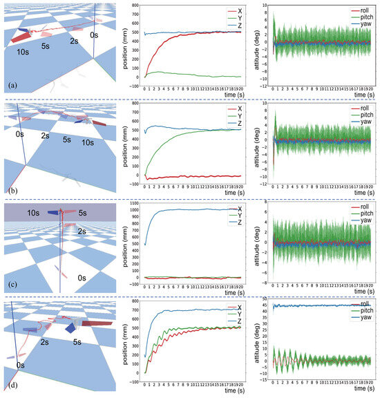
Figure 12.
Each experiment is presented in a separate row of images, including snapshots at specific moments, position, and attitude information. (a) Flight and hover along the x-axis. (b) Flight and hover along the y-axis. (c) Flight and hover along the z-axis. (d) Diagonal point-to-point flight.
It is worth noting that directly training for these long-distance point-to-point flights is rather difficult. The drone must learn to accelerate for takeoff and then decelerate to hover. If the starting and target positions are set as far apart as in this section during training, it often results in failures. However, this kind of trianing task is relatively easy for quadcopters with greater control authority [43].
4.4. Trajectory Tracking
The trained policy can be used for trajectory tracking. Figure 13 illustrates the drone tracking a circle parallel to the horizontal plane ith a radius of 300 mm. The target position setpoint is changed every 600 control steps and it is set to a point tangent to the trajectory in order to accelerate the tracking speed.
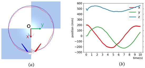
Figure 13.
Tracking a circular trajectory. (a) Top view. (b) Spatial position information.
4.5. Multi-Drones
This section demonstrates implementation of controlled flight of multiple drones in a simulated environment. Figure 14a shows multiple drones hovering at different vertex positions of a 300 mm edge length cube in space. Figure 14b presents two images showing eight drones taking off from a height of 200 mm to hover at 750 mm, each with a different initial yaw angle, while maintaining a circular formation during the flight.
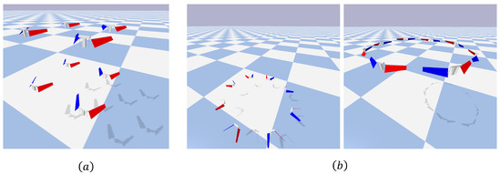
Figure 14.
Control of multiple FWMAVs: (a) Cubic formation (b) Circular formation.
During training, the FWMAV always takes off from a stationary state, but our hovering policy can be applied to drones with non-zero initial velocity. To demonstrate this, eight FWMAVs are initially positioned at the same height of 750 mm, and the 0th FWMAV is applied the trained control voltage signal, while the 1st to 7th FWMAVs are allowed to free fall under gravity. The control voltage is applied to the 1st FWMAV after the 0th FWMAV has been controlled for 20 control steps, then to the 2nd FWMAV after the 1st FWMAV has been controlled for 20 control steps, and so on. As shown in Figure 15, all eight drones eventually return to hovering at the height of 750 mm.
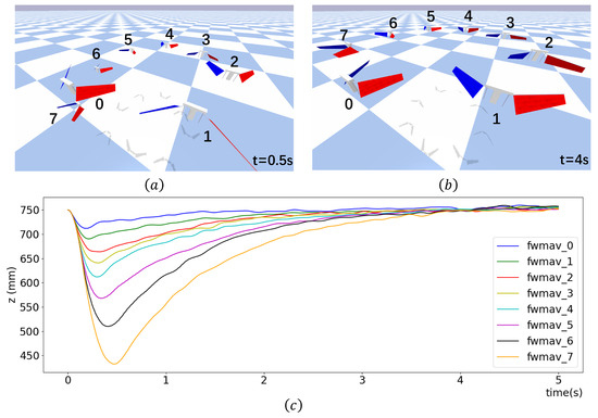
Figure 15.
Applying the trained controller to various FWMAVs at different time. (a,b) The positions of 8 FWMAVs at specific moments. (c) The variation in flight altitude of the FWMAVs over 5 s.
5. Conclusions
This paper utilizes deep reinforcement learning to train a hovering strategy for a Bi-directional Motor Driven FWMAV. The strategy operates at a low-level, directly mapping the FWMAV’s state to motor voltage outputs. We select appropriate action and state spaces, design a reward function to maintain attitude stability during flapping flight within a confined space, and train using the PPO algorithm across 20 parallel simulation environments. Verification in high-fidelity simulation environments demonstrates its applicability for FWMAV pose control, enabling agile transitions from forward flight, lateral flight, or liftoff to hovering, facilitating point-to-point movement. Additionally, simple trajectory tracking and multi-drone formation flight are demonstrated. Future work will focus on sim-to-real transfer, particularly addressing sensor noise and safety concerns, with the aim of deploying the strategy onto real FWMAVs in laboratory.
6. Notation
Because different fields have their own conventional symbols, which may conflict and cause confusion in this manuscript, we include this section to clarify the potentially confusing symbols. Below are the notation in different contexts:
| r | Aerodynamics: Radial wing distance |
| Reinforcement Learning: Rewards (typically with a time-series subscript) | |
| R | Aerodynamics: Wing span |
| Reinforcement Learning: Return | |
| , | Drone Euler Angles: Roll angle () and yaw angle () |
| Wing Motion: Stroke angle and rotation angle (typically with subscript w) | |
| Drone Euler Angles: Pitch angle | |
| Policy Learning: Parameters to be optimized in the policy | |
| Drone State: Body angular velocity | |
| Actor-Critic Algorithm: Parameters of the value network |
Author Contributions
Conceptualization, H.H. and Z.Z.; methodology, H.H.; software, H.H. and Z.Z.; validation, H.H.; formal analysis, H.H.; writing—original draft preparation, H.H.; writing—review and editing, H.H. and Z.Z.; visualization, H.H.; supervision, Z.W. and X.W.; project administration, Z.W. and X.W. All authors have read and agreed to the published version of the manuscript.
Funding
This research is supported in part by the Colleges and Universities Stable Support Project of Shenzhen, China, (No. GXWD20220811173149002), in part by the Guangdong Provincial Key Laboratory of Novel Security Intelligence Technologies under Grant 2022B1212010005.
Data Availability Statement
The code is available at https://github.com/huajuaner/QY-hummingbird (accessed on 18 September 2024).
Conflicts of Interest
The authors declare no conflicts of interest.
Abbreviations
The following abbreviations are used in this manuscript:
| FWMAV | Flapping Wing Micro Aerial Vehicle |
| PD | Proportional-Derivative |
| DDPG | Deep Deterministic Policy Gradient |
| PPO | Proximal Policy Optimization |
| URDF | Unified Robot Description Format |
| GAE | Generalized Advantage Estimation |
| A2C | Advantage Actor-Critic |
References
- Wasserman, D.H. How hummingbirds hover: Natural selection for energetics of hovering flight. Mol. Cell 2023, 83, 827–828. [Google Scholar] [CrossRef] [PubMed]
- Kajak, K.M.; Karásek, M.; Chu, Q.P.; De Croon, G.C.H.E. A minimal longitudinal dynamic model of a tailless flapping wing robot for control design. Bioinspir. Biomimetics 2019, 14, 046008. [Google Scholar] [CrossRef]
- Nabawy, M.R.; Crowther, W.J. Is flapping flight aerodynamically efficient? In Proceedings of the 32nd AIAA Applied Aerodynamics Conference, Atlanta, GA, USA, 16–20 June 2014. [Google Scholar]
- Tanaka, S.; Asignacion, A.; Nakata, T.; Suzuki, S.; Liu, H. Review of biomimetic approaches for drones. Drones 2022, 6, 320. [Google Scholar] [CrossRef]
- Floreano, D.; Wood, R.J. Science, technology and the future of small autonomous drones. Nature 2015, 521, 460–466. [Google Scholar] [CrossRef]
- de Croon, G. Science, Flapping wing drones show off their skills. Sci. Robot. 2020, 5, eabd0233. [Google Scholar] [CrossRef]
- Karásek, M.; Muijres, F.T.; De Wagter, C.; Remes, B.D.; De Croon, G.C. A tailless aerial robotic flapper reveals that flies use torque coupling in rapid banked turns. Science 2018, 361, 1089–1094. [Google Scholar] [CrossRef]
- Phan, H.V.; Aurecianus, S.; Kang, T.; Park, H.C. KUBeetle-S: An insect-like, tailless, hover-capable robot that can fly with a low-torque control mechanism. Int. J. Micro Air Veh. 2019, 11, 1756829319861371. [Google Scholar] [CrossRef]
- Chin, Y.W.; Kok, J.M.; Zhu, Y.Q.; Chan, W.L.; Chahl, J.S.; Khoo, B.C.; Lau, G.K. Efficient flapping wing drone arrests high-speed flight using post-stall soaring. Sci. Robot. 2020, 5, eaba2386. [Google Scholar] [CrossRef]
- Ma, K.Y.; Chirarattananon, P.; Fuller, S.B.; Wood, R.J. Controlled flight of a biologically inspired, insect-scale robot. Science 2013, 340, 603–607. [Google Scholar] [CrossRef]
- Tu, Z.; Fei, F.; Zhang, J.; Deng, X. An at-scale tailless flapping-wing hummingbird robot. I. Design, optimization, and experimental validation. IEEE Trans. Robot. 2020, 36, 1511–1525. [Google Scholar] [CrossRef]
- Hines, L.; Campolo, D.; Sitti, M. Liftoff of a motor-driven, flapping-wing microaerial vehicle capable of resonance. IEEE Trans. Robot. 2013, 30, 220–232. [Google Scholar] [CrossRef]
- Doman, D.B.; Oppenheimer, M.W.; Sigthorsson, D.O. Wingbeat shape modulation for flapping-wing micro-air-vehicle control during hover. J. Guid. Control Dyn. 2010, 33, 724–739. [Google Scholar] [CrossRef]
- Zhang, J.; Tu, Z.; Fei, F.; Deng, X. Geometric flight control of a hovering robotic hummingbird. In Proceedings of the IEEE International Conference on Robotics and Automation (ICRA), Singapore, 29 May–3 June 2017; pp. 5415–5421. [Google Scholar]
- Phan, H.V.; Kang, T.; Park, H.C. Design and stable flight of a 21 g insect-like tailless flapping wing micro air vehicle with angular rates feedback control. Bioinspir. Biomimetics 2017, 12, 036006. [Google Scholar] [CrossRef]
- Chirarattananon, P.; Ma, K.Y.; Wood, R.J. Adaptive control of a millimeter-scale flapping-wing robot. Bioinspir. Biomimetics 2014, 9, 025004. [Google Scholar] [CrossRef]
- Chirarattananon, P.; Ma, K.Y.; Wood, R.J. Perching with a robotic insect using adaptive tracking control and iterative learning control. Int. J. Robot. Res. 2016, 35, 1185–1206. [Google Scholar] [CrossRef]
- Fei, F.; Tu, Z.; Zhang, J.; Deng, X. Learning extreme hummingbird maneuvers on flapping wing robots. In Proceedings of the 2019 International Conference on Robotics and Automation (ICRA), Montreal, QC, Canada, 20–24 May 2019; pp. 109–115. [Google Scholar]
- Tu, Z.; Fei, F.; Deng, X. Bio-inspired rapid escape and tight body flip on an at-scale flapping wing hummingbird robot via reinforcement learning. IEEE Trans. Robot. 2021, 37, 1742–1751. [Google Scholar] [CrossRef]
- Nozawa, T.; Nakamura, K.; Katsuyama, R.; Kuwajima, S.; Li, Z.; Nomizu, A.; Watanabe, T. The wifly: Flapping-wing small unmanned aerial vehicle with center-of-gravity shift mechanism. J. Robot. Mechatronics 2021, 33, 205–215. [Google Scholar] [CrossRef]
- Lee, T.; Mckeever, S.; Courtney, J. Flying free: A research overview of deep learning in drone navigation autonomy. Drones 2021, 5, 52. [Google Scholar] [CrossRef]
- Kaufmann, E.; Bauersfeld, L.; Loquercio, A.; Müller, M.; Koltun, V.; Scaramuzza, D. Champion-level drone racing using deep reinforcement learning. Nature 2023, 620, 982–987. [Google Scholar] [CrossRef]
- Koch, W.; Mancuso, R.; West, R.; Bestavros, A. Reinforcement learning for UAV attitude control. ACM Trans. Cyber-Phys. Syst. 2019, 3, 1–21. [Google Scholar] [CrossRef]
- Molchanov, A.; Chen, T.; Hönig, W.; Preiss, J.A.; Ayanian, N.; Sukhatme, G.S. Sim-to-(multi)-real: Transfer of low-level robust control policies to multiple quadrotors. In Proceedings of the IEEE/RSJ International Conference on Intelligent Robots and Systems (IROS), Macau, China, 3–8 November 2019; pp. 59–66. [Google Scholar]
- Ibarz, J.; Tan, J.; Finn, C.; Kalakrishnan, M.; Pastor, P.; Levine, S. How to train your robot with deep reinforcement learning: Lessons we have learned. Int. J. Robot. Res. 2021, 40, 698–721. [Google Scholar] [CrossRef]
- Campolo, D.; Azhar, M.; Lau, G.K.; Sitti, M. Can DC motors directly drive flapping wings at high frequency and large wing strokes? IEEE ASME Trans. Mechatronics 2012, 19, 109–120. [Google Scholar] [CrossRef]
- Zhang, J.; Deng, X. Resonance principle for the design of flapping wing micro air vehicles. IEEE Trans. Robot. 2017, 33, 183–197. [Google Scholar] [CrossRef]
- Whitney, J.P.; Wood, R.J. Aeromechanics of passive rotation in flapping flight. J. Fluid Mech. 2010, 660, 197–220. [Google Scholar] [CrossRef]
- Dickinson, M.H.; Lehmann, F.O.; Sane, S.P. Wing rotation and the aerodynamic basis of insect flight. Science 1999, 284, 1954–1960. [Google Scholar] [CrossRef]
- Ellington, C.P. The aerodynamics of hovering insect flight. II. Morphological parameters. Philos. Trans. R. Soc. Lond. B Biol. Sci. 1984, 305, 17–40. [Google Scholar]
- Dickson, W.; Straw, A.; Poelma, C.; Dickinson, M. An integrative model of insect flight control. In Proceedings of the 44th AIAA Aerospace Sciences Meeting and Exhibit, Reno, NV, USA, 9–12 January 2006; p. 34. [Google Scholar]
- Hassan, K.K. Nonlinear Systems, 3rd ed.; Prentice Hall: Upper Saddle River, NJ, USA, 2002; pp. 381–419. [Google Scholar]
- Zhang, J.; Cheng, B.; Deng, X. Instantaneous wing kinematics tracking and force control of a high-frequency flapping wing insect MAV. J. Micro-Bio Robot. 2016, 11, 67–84. [Google Scholar] [CrossRef]
- Sutton, R.S. Reinforcement Learning: An Introduction, 2nd ed.; A Bradford Book; MIT Press: Cambridge, MA, USA, 2018; pp. 56–88. [Google Scholar]
- Sutton, R.S.; McAllester, D.; Singh, S.; Mansour, Y. Policy gradient methods for reinforcement learning with function approximation. In Advances in Neural Information Processing Systems 12; MIT Press: Cambridge, MA, USA, 1999. [Google Scholar]
- Schulman, J.; Wolski, F.; Dhariwal, P.; Radford, A.; Klimov, O. Proximal policy optimization algorithms. arXiv 2017, arXiv:1707.06347. [Google Scholar]
- Schulman, J.; Moritz, P.; Levine, S.; Jordan, M.; Abbeel, P. High-dimensional continuous control using generalized advantage estimation. arXiv 2015, arXiv:1506.02438. [Google Scholar]
- PyBullet, a Python Module for Physics Simulation for Games, Robotics and Machine Learning. Available online: http://pybullet.org (accessed on 30 May 2024).
- Kaufmann, E.; Bauersfeld, L.; Scaramuzza, D. A benchmark comparison of learned control policies for agile quadrotor flight. In Proceedings of the International Conference on Robotics and Automation (ICRA), Philadelphia, PA, USA, 23–27 May 2022; pp. 10504–10510. [Google Scholar]
- Raffin, A.; Hill, A.; Gleave, A.; Kanervisto, A.; Ernestus, M.; Dormann, N. Stable-Baselines3: Reliable Reinforcement Learning Implementations. J. Mach. Learn. Res. 2021, 22, 1–8. [Google Scholar]
- Mnih, V. Asynchronous methods for deep reinforcement learning. arXiv 2016, arXiv:1602.01783. [Google Scholar]
- Lillicrap, T.P. Continuous control with deep reinforcement learning. arXiv 2015, arXiv:1509.02971. [Google Scholar]
- Panerati, J.; Zheng, H.; Zhou, S.; Xu, J.; Prorok, A.; Schoellig, A.P. Learning to fly—A gym environment with pybullet physics for reinforcement learning of multi-agent quadcopter control. In Proceedings of the IEEE/RSJ International Conference on Intelligent Robots and Systems (IROS), Prague, Czech Republic, 27 September–1 October 2021; pp. 7512–7519. [Google Scholar]
Disclaimer/Publisher’s Note: The statements, opinions and data contained in all publications are solely those of the individual author(s) and contributor(s) and not of MDPI and/or the editor(s). MDPI and/or the editor(s) disclaim responsibility for any injury to people or property resulting from any ideas, methods, instructions or products referred to in the content. |
© 2024 by the authors. Licensee MDPI, Basel, Switzerland. This article is an open access article distributed under the terms and conditions of the Creative Commons Attribution (CC BY) license (https://creativecommons.org/licenses/by/4.0/).