UAV Confrontation and Evolutionary Upgrade Based on Multi-Agent Reinforcement Learning

Abstract

Unmanned aerial vehicle (UAV) confrontation scenarios play a crucial role in the study of agent behavior selection and decision planning. Multi-agent reinforcement learning (MARL) algorithms serve as a universally effective method guiding agents toward appropriate action strategies. They determine subsequent actions based on the state of the agents and the environmental information that the agents receive. However, traditional MARL settings often result in one party agent consistently outperforming the other party due to superior strategies, or both agents reaching a strategic stalemate with no further improvement. To solve this issue, we propose a semi-static deep deterministic policy gradient algorithm based on MARL. This algorithm employs a centralized training and decentralized execution approach, dynamically adjusting the training intensity based on the comparative strengths and weaknesses of both agents’ strategies. Experimental results show that during the training process, the strategy of the winning team drives the losing team’s strategy to upgrade continuously, and the relationship between the winning team and the losing team keeps changing, thus achieving mutual improvement of the strategies of both teams. The semi-static reinforcement learning algorithm improves the win-loss relationship conversion by 8% and reduces the training time by 40% compared with the traditional reinforcement learning algorithm.

1. Introduction

In recent years, many researchers have studied multi-agent confrontation widely, which is an important multi-agent research direction [1,2,3,4,5]. Multi-agent confrontation mainly involves the combination of autonomous agents into two groups for group confrontation. During the confrontation, the two groups of agents constantly adjust their actions based on the information they obtain in order to defeat their opponents. The information they acquire includes their own status information, the acquired surrounding environment information, and the other agent status information, etc. Reference [6] introduces the multi-agent deep reinforcement learning paradigm into the confrontation scene of an unmanned aerial vehicle (UAV) swarm and constructs two UAV swarm non-cooperative game models based on the multi-agent deep deterministic policy gradient (MADDPG) algorithm and the multi-agent soft actor-critic algorithm. Reference [7] presents a new bio-inspired decision-making method for UAV swarms for attack-defense confrontation via multi-agent reinforcement learning (MARL). Reference [8] proposes a large-scale multi-agent evolutionary reinforcement joint method, which divides the multi-agent learning task into multiple stages according to the size of the agent, and uses the self-attention mechanism to handle changing numbers of agents in each step.

The authenticity of adversarial environments [9,10] and multi-agent control [11,12] is significant for real-world scenarios. Meanwhile, MARL [13,14,15,16,17], as an effective training method for multiple agents, is widely employed in multi-agent confrontation.

Reinforcement learning enables agents to make decisions based on their own state information and environmental information to improve their strategies, offering an effective method for realizing realistic adversarial scenarios. Agents evaluate the effectiveness of their decisions based on environmental feedback and update their strategies accordingly. Through continuous action, learning, and updating of behaviors, the behaviors of both groups gradually approximate a real adversarial scenario to accomplish predefined tasks.

In the academic community, there are three basic solution paradigms for the MARL algorithm:

• Fully centralized methods: the fully centralized methods treat the decisions of multiple agents as those of a super-agent, aggregating the states of all agents into a global super-state and connecting the actions of all agents as a joint action. While advantageous for the super-agent as the environment remains static, ensuring the convergence of individual agent algorithms, this method struggles to scale well with a large number of agents or a large environment due to the curse of dimensionality [18].
• Fully decentralized methods: the fully decentralized methods assume each agent learns independently in its own environment without considering changes in other agents, such as independent proximal policy optimization (IPPO) algorithm [19]. Each agent applies a single-agent reinforcement learning algorithm directly. This method exhibits good scalability with increasing agent numbers without encountering training termination due to the curse of dimensionality. However, the environment using this method is non-stationary, jeopardizing the convergence of training.
• Centralized Training Decentralized Execution (CTDE): CTDE utilizes global information, which individual agents cannot observe during training, to achieve better training performance. However, during execution, this global information is not used, and each agent takes actions solely based on its own policy, thus achieving decentralized execution. CTDE algorithms effectively use global information to enhance the quality and stability of training, while only using local information during policy model inference, making the algorithm scalable to a certain extent.

CTDE algorithms mainly consist of two types: value function-based methods such as Value-Decomposition Networks (VDN) [20], monotonic value function factorization for deep multi-agent reinforcement learning (QMIX) [21], and actor-critic-based methods such as MADDPG [22] and counterfactual multi-agent policy gradients (COMA) [23].

Traditional multi-agent adversarial algorithms often involve both sides updating their strategies, which cannot achieve realistic adversarial effects. Reference [24] proposes a multi-phase semi-static training method for swarm confrontation using MARL. Reference [25] proposes a novel multi-agent hierarchical policy gradient algorithm, which is capable of learning various strategies and transcending expert cognition by adversarial self-play learning. To achieve realistic UAV confrontation effects, we propose a new semi-static reinforcement learning algorithm.

In addition to training the agent strategies by using the new semi-static reinforcement learning algorithm, we also employ a path planning and obstacle avoidance algorithm to enable agents to execute corresponding actions. Ref. [26] presents a unique real-time obstacle avoidance approach for mobile robots based on the artificial potential field. Ref. [27] proposes a heuristic search algorithm, which is widely used for path planning and obstacle avoidance. In this paper, we use the disturbance flow field method for agent path planning and obstacle avoidance because the path planned by this method is smooth and easy to track, and this method has high computational efficiency and a small path cost [28].

This paper constructs a completely fair multi-agent confrontation scenario, that is, the initial state, number, and environmental information of the two groups are exactly the same. When we use the traditional MARL algorithm to train two groups of agents, the final experimental results are unsatisfactory. After the two groups continue to compete and evolve, it is very common for one group’s strategy to completely outperform the other’s, or for the two groups’ strategies to reach a dynamic balance and no longer improve the strategies. This greatly limits the exploration and improvement of the reinforcement learning algorithm strategies in multi-agent confrontation scenarios. This phenomenon causes the two groups of agents to fail to learn optimal behavioral decisions.

The experimental results of training two groups of agents with the traditional MARL algorithm show that the training time of the two groups is too long and the ability difference between the two groups is too large. The win-loss relationship between the two groups is not frequent, and the effect of mutual promotion and mutual improvement cannot be achieved. However, this paper proposes a multi-agent confrontation method based on semi-static reinforcement learning. In the completely fair multi-agent confrontation environment, through semi-static reinforcement learning, the strategies of the two groups of agents can be improved alternately, and the intelligence can be gradually enhanced, which is closer to the real confrontation environment. The experimental results show that this method can significantly shorten the training time of the two intelligent groups and reduce the ability gap between both groups. The win-loss relationship between the two groups changes more frequently, and the intelligence is improved. We also verify the authenticity and effectiveness of the algorithm by changing the simulation environment. At the same time, through the disturbance flow field method, agents can perform path planning and obstacle avoidance behaviors during adversarial processes, facilitating cooperative interaction among agents.

The rest of this paper is organized as follows: In Section 2, we give the physical constraints of the drone dynamic model and illustrate the principles of the path planning algorithm. In Section 3, we construct a UAV confrontation scenario and design a semi-static deep deterministic policy gradient algorithm based on MARL. In Section 4, we conduct simulation experiments, obtain experimental conclusions and compare our algorithm with the original algorithm. Finally, in Section 5, we conclude this article and draw some prospects.

2. Model Constraints and Path Planning

2.1. Drone Dynamic Model

In order to express briefly,

Table 1. Important Symbol Definitions.

Symbol	Definitions
$i,j\in \left\{1,\cdots ,n\right\}$	The indexes of drones
$i,j\in \left\{1,\cdots ,m\right\}$	The indexes of obstacles
$p_u^i$	The position of drone i
$p_o^i$	The position of obstacle i
$p_e^i$	The destination of drone i
$v_u^i$	The velocity of drone i
$v_o^i$	The velocity of obstacle i
${\rho }_u$	The geometric radius of drone
${\rho }_o$	The geometric radius of cylindrical obstacle
H	The geometric height of cylindrical obstacle
${\chi }_u$	The detection angle of drone
$R_u$	The detection radius of drone
$B_u^i$	The blood of drone i
${\psi }_u^i$	The roll angle of drone i
${\theta }_u^i$	The yaw angle of drone i
${\phi }_u^i$	The pitch angle of drone i
$s,s^{\prime }$	The state
z	The observation
a	The action
r	The reward
S	The state space
Z	The observation space
A	The action space
$\gamma$	The discount factor

provides the definitions of the important symbols.

In this paper, we consider a group of n drones labeled as $i,j\in \left\{1,\cdots ,n\right\}$, and m obstacles labelled as $i,j\in \left\{1,\cdots ,m\right\}$. We model each drone as a sphere. The position and velocity of drone i are denoted by $p_u^i,v_u^i\in {\mathbb{R}}^3$, respectively. The position and velocity of obstacle i are denoted by $p_o^i,v_o^i\in {\mathbb{R}}^3$, respectively. The geometric radius of the drone and the cylindrical obstacle are defined as ${\rho }_u$ and ${\rho }_o$, respectively. The geometric height of the cylindrical obstacle is defined as H. Since both drones and obstacles have geometric shapes, the distance between drone i and drone j should be less than twice the geometric radius of the drone during drone path planning. The distance between drones and obstacles should be less than the algebraic sum of the geometric radius of the drone and the geometric radius of the obstacle.

Each drone has a detection radius $R_u$ and a detection angle ${\chi }_u$ due to its detection and attack capabilities. If drone i is within the detection radius and detection angle of drone j, drone j will attack drone i. Each drone has the blood $B_u^i$. When drone i is hit, $B_u^i$ reduces the number by one. When $B_u^i$ reduces to zero, drone i is destroyed.

We need to impose some physical condition constraints on the drone dynamic model due to the movement of drone is in three-dimensional space. In order to ensure the stability and safety of the drone flight, we constrain the yaw angle and pitch angle of the drone; in order to ensure that the drone does not change its flight direction frequently, we set a constraint on the shortest flight distance of the drone; in order to ensure that the drone does not leave the experimental environment, we restrict the flight height of the drone and in order to ensure the smooth completion of the experiment, we set constraints on the total flight distance of the drone.

Here, $p_u^i\left(t\right)$ represents the position of drone i at time t, and $x,y,z$ represent the position of drone i in the three-dimensional space. Considering three consecutive positions $p_u^i(t-1),p_u^i\left(t\right),p_u^i(t+1)$, the constraints on the drone i’s three-dimensional trajectory can be specified as follows:

• Yaw Angle Constraint: the drone can only turn on a horizontal plane that is less than or equal to the specified maximum yaw angle:

  $$\begin{array}{c}{\theta }_t=arccos{\displaystyle \frac{\left(x_{t+1}-x_t\right)\left(x_t-x_{t-1}\right)+\left(y_{t+1}-y_t\right)\left(y_t-y_{t-1}\right)}{\sqrt{{\left(x_{t+1}-x_t\right)}^2+{\left(y_{t+1}-y_t\right)}^2}·\sqrt{{\left(x_t-x_{t-1}\right)}^2+{\left(y_t-y_{t-1}\right)}^2}}}\end{array}$$

  (1)
  In the above formula, ${\theta }_t\le {\theta }_{\max }$, where ${\theta }_{\max }$ denotes the maximum yaw angle.
• Pitch Angle Constraint: the drone can only rise in a vertical plane that is less than or equal to the specified maximum pitch angle:

  $$\begin{array}{c}{\phi }_t=arctan{\displaystyle \frac{\left|z_t-z_{t-1}\right|}{\sqrt{{\left(x_t-x_{t-1}\right)}^2+{\left(y_t-y_{t-1}\right)}^2}}}\end{array}$$

  (2)
  In the above formula, ${\phi }_t\le {\phi }_{\max }$, where ${\phi }_{\max }$ denotes the maximum pitch angle.
• The Trajectory Segment Length Constraint represents the shortest distance that the drone can fly along the current flight direction before changing its flight attitude.

  $$\begin{array}{c}{L}_t=\sqrt{{\left(x_t-x_{t-1}\right)}^2+{\left(y_t-y_{t-1}\right)}^2+{\left(z_t-z_{t-1}\right)}^2}\end{array}$$

  (3)
  In the above formula, $L_t\ge L_{\min }$, where $L_{\min }$ denotes the minimum segment length of the trajectory.
• Flight Height Constraint represents the height of the drone that the drone can safely fly.

  $$\begin{array}{c}{z}_{min}\le z_t\le z_{max}\end{array}$$

  (4)
  In the above formula, $z_{\max }$ represents the maximum height, while $z_{\min }$ represents the minimum height.
• The Total Trajectory Length Constraint is the total trajectory length of the drone less than or equal to the specified threshold.

  $$\begin{array}{c}\sum _{t=1}^T{L}_t\le L_{max}\end{array}$$

  (5)
  In the above formula, $L_{\max }$ represents the maximum total trajectory length.

2.2. Disturbance Flow Field Method

The disturbance flow field method is an algorithm used for path planning and obstacle avoidance, particularly suitable for agents to solve motion planning problems encountered in complex environments. In the disturbance flow field method, the environment is conceptualized as a fluid or gas, while the controlled entities are regarded as objects moving within this flow field. In this paper, we model the adversarial environment for multi-agent as a flow field, with each drone treated as an object moving within this flow field. We introduce cylindrical obstacles into the designed adversarial environment and model each drone as a sphere. To describe the impact of the obstacle on the initial flow field, we define that the position of drone i is $x,y,z$ in the three-dimensional space. For the obstacles, the following equations can be established:

$$\begin{array}{c}F\left(i\right)={\left({\displaystyle \frac{x-x_0}{a}}\right)}^{2d}+{\left({\displaystyle \frac{y-y_0}{b}}\right)}^{2e}+{\left({\displaystyle \frac{z-z_0}{c}}\right)}^{2f}\end{array}$$

(6)

In the above formula, $x_0,y_0,z_0$, respectively, represent the position of the geometric center of the obstacle in the three-dimensional space. If the obstacle is a sphere, $a=b=c=R$ and $d=1, e=1, f=1$, R is the radius of the sphere; if the obstacle is a cylinder, $a=b=R$, $c={\displaystyle \frac{H}{2}}$ and $d=1, e=1, f>1$, R is the radius of the cylinder and H is the height of the cylinder.

We assume the speed of drone i is a constant C, and the destination of drone i is $x_{\mathrm{d}}, y_{\mathrm{d}}, z_{\mathrm{d}}$ in the three-dimensional space; the original fluid velocity $v\left(i\right)$ can be described as:

$$\begin{array}{c}v\left(i\right)={\left[{\displaystyle \frac{C(x-x_{\mathrm{d}})}{d\left(i\right)}},{\displaystyle \frac{C(y-y_{\mathrm{d}})}{d\left(i\right)}},{\displaystyle \frac{C(z-z_{\mathrm{d}})}{d\left(i\right)}}\right]}^{\mathrm{T}}\end{array}$$

(7)

where $d\left(i\right)=\sqrt{{\left(x-x_{\mathrm{d}}\right)}^2+{\left(y-y_{\mathrm{d}}\right)}^2+{\left(z-z_{\mathrm{d}}\right)}^2}$ is the distance between the position of drone i and the destination of drone i.

The effect of obstacles on the original fluid can be quantified by the perturbation matrix $P\left(i\right)$. The perturbation matrix $P\left(i\right)$ is defined as:

$$\begin{array}{c}P\left(i\right)=I-{\displaystyle \frac{n\left(i\right)n{\left(i\right)}^T}{{\left|F\left(i\right)\right|}^{\frac{1}{\rho \left(i\right)}}n{\left(i\right)}^{T}n\left(i\right)}}+{\displaystyle \frac{\tau m\left(i\right)n{\left(i\right)}^T}{{\left|F\left(i\right)\right|}^{\frac{1}{\sigma \left(i\right)}}\parallel m\left(i\right)\parallel \parallel n\left(i\right)\parallel }}\end{array}$$

(8)

In the above formula, I is an identity matrix, $n\left(i\right)$ and $m\left(i\right)$ are the normal vector and tangential vector, respectively, $\tau$ is the saturation function of the tangential velocity $\parallel ·\parallel$, and is the two norms of a vector or a matrix. Besides, $\rho \left(i\right)$ and $\sigma \left(i\right)$ are the weights of $n\left(i\right)$ and $m\left(i\right)$, respectively. Their definitions are as follows:

$$\begin{array}{c}n\left(i\right)={\left[{\displaystyle \frac{\partial F\left(i\right)}{\partial x}}{\displaystyle \frac{\partial F\left(i\right)}{\partial y}}{\displaystyle \frac{\partial F\left(i\right)}{\partial z}}\right]}^T\end{array}$$

(9)

$$\begin{array}{c}m\left(i\right)={\left[\begin{array}{ccc}{\displaystyle \frac{\partial F\left(i\right)}{\partial x}}& -{\displaystyle \frac{\partial F\left(i\right)}{\partial y}}& 0\end{array}\right]}^T\end{array}$$

(10)

$$\begin{array}{c}\rho \left(i\right)={\rho }_{0}exp\left(1-{\displaystyle \frac{1}{d_0\left(i\right)d\left(i\right)}}\right)\end{array}$$

(11)

$$\begin{array}{c}\sigma \left(i\right)={\sigma }_{0}exp\left(1-{\displaystyle \frac{1}{d_0\left(i\right)d\left(i\right)}}\right)\end{array}$$

(12)

$$\begin{array}{c}\tau =\left\{\begin{array}{cc}1\hfill & V\left(i\right)>\overline{\varsigma }\hfill \\ {\displaystyle \frac{V\left(i\right)}{\overline{\varsigma }}}\hfill & -\overline{\varsigma }\le V\left(i\right)\le \overline{\varsigma }\hfill \\ -1\hfill & V\left(i\right)<-\overline{\varsigma }\hfill \end{array}\right.\end{array}$$

(13)

In the above formulas, $V\left(i\right)=v{\left(i\right)}^{T}m\left(i\right)n{\left(i\right)}^{T}v\left(i\right)$, ${\rho }_0$ is the repulsion parameter, ${\sigma }_0$ is the tangential parameter, $d_0\left(i\right)$ is the distance between the boundary of the obstacle and the current position of drone i, and $\overline{\varsigma }>0$ is the threshold that determines the saturation function $\tau$. The speed of the disturbed fluid and the position of drone i at the next moment can be calculated by the following formula:

$$\begin{array}{c}\overline{v}\left(i\right)=P\left(i\right)v\left(i\right)\end{array}$$

(14)

$$\begin{array}{c}{p}_u^i(t+1)=p_u^i\left(t\right)+\overline{v}\left(i\right)\Delta t\end{array}$$

(15)

where $p_u^i(t+1)$ and $p_u^i\left(t\right)$ represent the position of drone i at the next and current time steps, while $\Delta t$ is the time step used for iteration. Therefore, we can plan the obstacle avoidance path of drone i through the disturbance flow field method.

3. Simulation Scenario and Algorithm Design

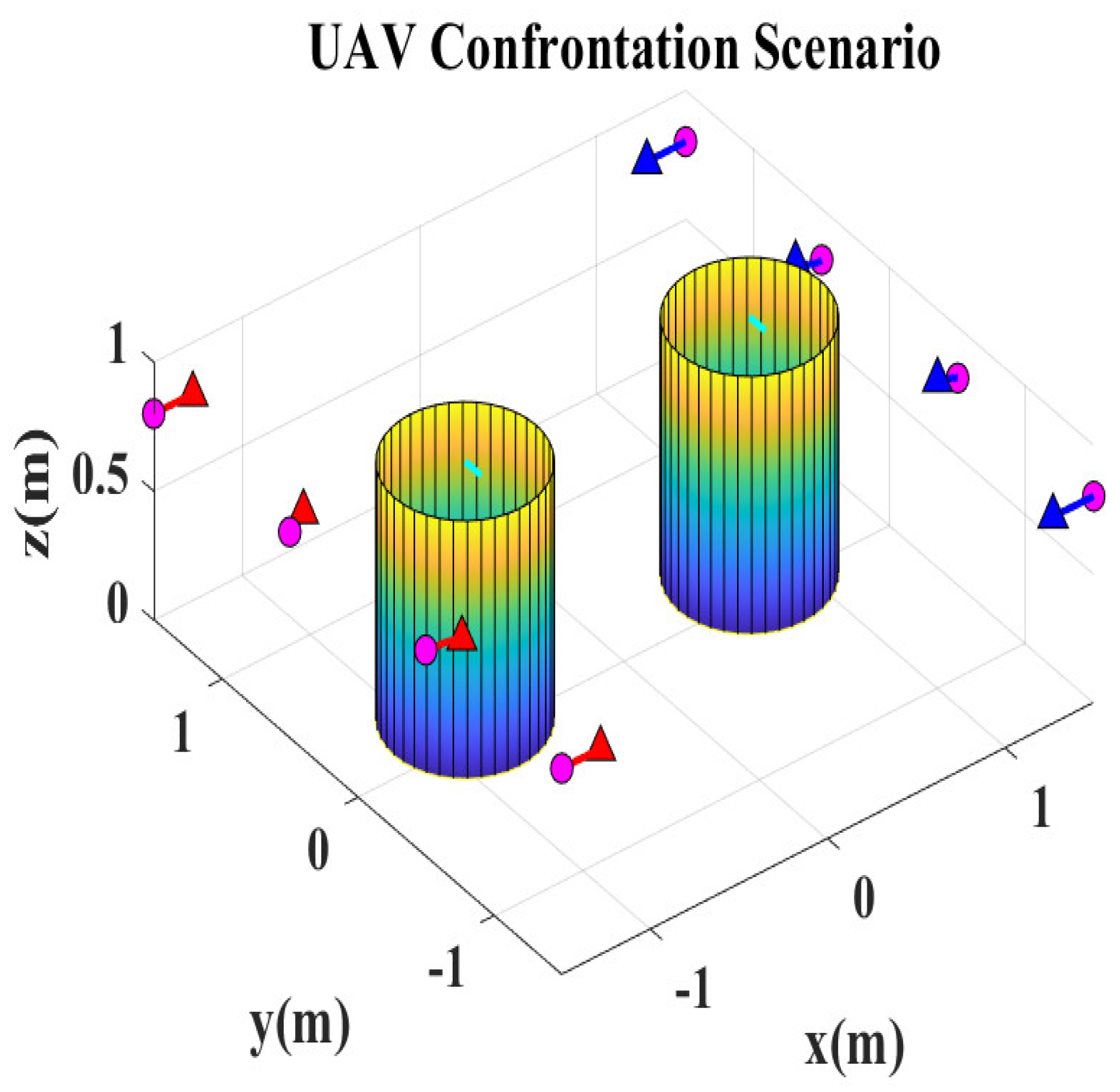
3.1. UAV Confrontation Scenario

This paper designs a UAV confrontation scenario with limited communication and environmental uncertainty. In this scenario, the blue team and the red team are scattered on both sides of the dynamic obstacles. The red team and the blue team each have four drones. The dynamic obstacles are cylinders. Figure 1 is the UAV confrontation scenario we design.

In Figure 1, each red triangle represents a red drone, and each blue triangle represents a blue drone. The pink dot represents both the starting position of the corresponding drone and the target position of the enemy drone. The dynamic cylindrical obstacles increase the uncertainty of the environmental information.

Each drone’s final task is to destroy the enemy drone and reach the given target point. At the same time, they need to complete three tasks: (1) Avoid the dynamic obstacles and other drones; (2) Maximize the opponent’s exposure to its own attack range; (3) Minimize exposure to enemy drones’ attacks. Both teams start with identical initial states, and each drone has its own blood. Drones in the same team cooperate with each other, while those from different teams compete. Because communication is restricted, the drone cannot communicate with the central planner, and each drone can only have limited communication. Therefore, each drone can only make decisions independently based on local observation information. The absence of a central planner makes it challenging for drones to balance their own rewards with those of the team, maximize team rewards, and minimize enemy rewards. Therefore, this scene is a confrontational task where cooperation and competition coexist.

In order to achieve the above tasks, we employ a MARL approach to train distributed policy networks for each drone, enabling them to make autonomous decisions. Each team achieves self-coordination based on the policies of its constituent drones.

3.2. Reinforcement Learning Algorithm Based on Actor-Critic

Reinforcement learning is a machine learning method aimed at enabling agents to learn behavioral decisions through interaction with the environment to maximize the expected cumulative rewards. To construct a multi-agent adversarial environment and train agents by using the MARL algorithm, we need to define the state space, action space, and reward function.

• State Space: The state space represents the state information of the constructed multi-agent adversarial environment, including both the agents’ own information and environmental information. It may include parameters such as the positions and velocities of the agents, the positions and velocities of adjacent agents, and the positions and velocities of obstacles.
• Action Space: The action space represents the actions that both agents of the multi-agent environment can take. In this case, the action space is represented by the actions performed by the agents. Based on the environmental conditions in the adversarial environment, agents may perform actions such as detecting and attacking.
• Reward Function: The reward function provides feedback to the agents after taking actions, guiding them toward better strategies and evaluating the system’s behaviors. It evaluates the goodness or badness of the system’s actions.

In this paper, we use the MADDPG algorithm based on actor-critic [29] as the decision-making algorithm. Two-party multi-agents can select the optimal actions based on the current observation information and continuously update their policy networks through the reward function to enhance their strategies progressively by using MADDPG. MADDPG is a CTDE algorithm and implements the DDPG algorithm [30] for each agent. All agents share a centralized critic network, which guides the actor network of each agent during training. During execution, each agent’s actor network makes decisions independently, achieving decentralized execution.

In MADDPG, each agent is trained using the actor-critic method. However, unlike in traditional single-agent scenarios, in MADDPG, each agent’s critic part can access the policy information of other agents.

Assuming n agents, with policy parameter $\theta =\{{\theta }_1,\dots ,{\theta }_n\}$ and policy set $\pi =\{{\pi }_1,\dots ,{\pi }_n\}$, the gradient of the expected return ${\nabla }_{{\theta }_i}J\left({\theta }_i\right)$ for agent i under stochastic policies is given by:

$$\begin{array}{c}{\nabla }_{{\theta }_i}J\left({\theta }_i\right)={\mathbb{E}}_{s\sim p^{\mu },a\sim {\pi }_i}[{\nabla }_{{\theta }_i}log{\pi }_i\left(a_i\right|o_i)Q_i^{\pi }(z,a)]\end{array}$$

(16)

where $Q_i^{\pi }(z,a)$ represents the centralized action-value function, z is the global state and a is the joint action of all agents. And $log{\pi }_i\left(a_i\right|o_i)$ represents the logarithmic probability that the agent i chooses the action $a_i$ according to its strategy ${\pi }_i$ given the observation $o_i$.

For deterministic policies, with n continuous policies ${\mu }_{{\theta }_i}$, the gradient ${\nabla }_{{\theta }_i}J\left({\mu }_i\right)$ is given by:

$$\begin{array}{c}{\nabla }_{{\theta }_i}J\left({\mu }_i\right)={\mathbb{E}}_{z,a\sim D}\left[{\nabla }_{{\theta }_i}{\mu }_i\left(o_i\right){\nabla }_{a_i}{Q}_i^{\mu }(z,a){|}_{a_i={\mu }_i\left(o_i\right)}\right]\end{array}$$

(17)

where D is the experience replay buffer storing data $(z,a,r,z^{\prime })$, ${\nabla }_{a_i}{Q}_i^{\mu }(z,a)$ represents the gradient of the centralized action-value function with respect to the policy parameters ${\theta }_i$.

In MADDPG, the centralized action-value function is updated using the following loss function:

$$\begin{array}{c}Ł\left({\theta }_i\right)={\mathbb{E}}_{z,a,r,z^{\prime }}\left[{(Q_i^{\mu }(z,a)-y_i)}^2\right]\end{array}$$

(18)

$$\begin{array}{c}{y}_i=r_i+\gamma Q_i^{{\mu }^{\prime }}(z^{\prime },a^{\prime }){|}_{a_j^{\prime }={\mu }_j^{\prime }\left(o_j\right)}\end{array}$$

(19)

where $Ł\left({\theta }_i\right)$ represents the loss function used to train the centralized action-value function, ${\mu }^{\prime }=({\mu }_{{\theta }_1}^{\prime },\dots ,{\mu }_{{\theta }_n}^{\prime })$ represents the target policy set, $y_i$ represents the target value, which is composed of the immediate reward $r_i$ and the discounted future value, $\gamma$ represents the discount factor used to calculate the current value of future rewards.

3.3. Semi-Static MADDPG Algorithm Based on UAV Confrontation Scenario

3.3.1. Observation Space and Action Space

MARL tasks, which may involve cooperation or competition, can be described by a partially observable Markov decision process [31,32,33,34]. We represent this with a tuple $\left(n,S,A,P,r,Z,O,\gamma \right)$ for n agents engaged in a Markov game, where $s\in S$ denotes the state of the environment. Here, $a_i\in A$ represents the action of each individual agent and $a\in A\equiv A^n$ is the set of joint action of all agents.

The transition function $P\left(s^{\prime }\right|s,a):S\times A\to S^{\prime }$ describes the state transitions from s to $s^{\prime }$ under the joint action a. The reward function $r(s,a):S\times A\to R$ quantifies the rewards. Each agent’s observation $z_i\in Z$ can be defined by the observation function $O(s,a):S\to Z$. The discount factor is denoted by $0<\gamma <1$. Each agent’s objective is to optimize its own policy network ${\pi }_i$ to maximize the cumulative reward. The expected cumulative reward $E_{{\mathsf{\Gamma }}_i\sim {\pi }_i}={\sum }_{t=1}^{\infty }{\gamma }_t{r}_t$, where $r_t\sim R_i$, can ultimately reach its maximum value. Here, ${\mathsf{\Gamma }}_i=\left(s_i\left(0\right),a_i\left(0\right),\cdots ,s_i\left(t\right),a_i\left(t\right)\right)$ represents the trajectory of each agent continuously interacting with the environment under its own policy, where $a_i\left(t\right)\sim {\pi }_i\left(·\mid z_i\left(t\right)\right)$ and $z_i(t+1)\sim P\left(·\mid z_i\left(t\right),a_i\left(t\right)\right)$ denote the optimal action chosen by agent i at time t and the observation at the next time step $t+1$, respectively.

Assume the confrontation scenario involving n drones and m dynamic obstacles. In this scenario, p and v, respectively, represent position and velocity vectors in a three-dimensional environment. $p_u^i$, $p_o^i$, and $p_e^i$, respectively, denote the position of the center of drone i, the center of obstacle i, and the destination of drone i. $v_u^i$ represents the velocity of drone i. $v_o^j$ represents the velocity of obstacle j. ${\rho }_u$ is the geometric radius of the drone and ${\rho }_o$ is the geometric radius of the dynamic obstacle. This scenario can be modeled as a partially observable Markov decision process, where each drone is considered a decision-making agent. The state space S of the entire scene contains the positional information of all drones and obstacles. The observation space Z for each drone includes its own position, the destination’s position, and the position and velocity of the nearest neighbor, which is a drone or a dynamic obstacle. The observation information for drone $i_1$ at time t can be expressed as:

If the nearest neighbor is a drone:

$$z_{i_1}\left(t\right)=\left[\begin{array}{c}{p}_e^{i_1}-p_u^{i_1}\\ v_u^{i_2}\\ (p_u^{i_2}-p_u^{i_1})·{\displaystyle \frac{d_{u_1{u}_2}^{i_1{i}_2}-2{\rho }_u}{d_{u_1{u}_2}^{i_1{i}_2}}}\end{array}\right]$$

(20)

If the nearest neighbor is a dynamic obstacle:

$$z_{i_1}\left(t\right)=\left[\begin{array}{c}{p}_e^{i_1}-p_u^{i_1}\\ v_o^j\\ (p_o^j-p_u^{i_1})·{\displaystyle \frac{d_{ou}^{i_{1}j}-({\rho }_o+{\rho }_u)}{d_{ou}^{i_{1}j}}}\end{array}\right]$$

(21)

where $d_{ou}^{i_{1}j}=\parallel {\overrightarrow{P}}_o^j-{\overrightarrow{P}}_u^{i_1}\parallel$ represents the distance from the center of drone $i_1$ to the center of obstacle j, and $d_{u_1{u}_2}^{i_1{i}_2}=\parallel {\overrightarrow{P}}_u^{i_1}-{\overrightarrow{P}}_u^{i_2}\parallel$ represents the distance from the center of drone $i_1$ to the center of drone $i_2$, using the Euclidean norm. This observational setup allows drones to operate completely distributed and autonomously without relying on a central planner. In the three-dimensional path planning problem, the action space for a drone can be expressed as:

$$\begin{array}{c}A={\left[{\psi }_u^i{\theta }_u^i{\phi }_u^i\right]}^T\end{array}$$

(22)

where ${\psi }_u^i$, ${\theta }_u^i$, and ${\phi }_u^i$ represent the roll, yaw, and pitch angles of each drone i. This action space is continuous. Based on the disturbance flow field algorithm, the position command of each drone i at the next moment can be calculated.

3.3.2. Algorithm Design

In implementing a multi-agent adversarial scenario using the MADDPG algorithm, each agent is equipped with four networks during training: the policy network, the target policy network, the value network, and the target value network. The policy network uses the agent’s local observations to output the optimal action decision, aiming to maximize the agent’s expected reward. The value network takes joint observations and joint actions of all agents as input, evaluating the output of the action by the agent’s policy network using a value function, thereby assisting in the training of the policy network. The target policy network and the target value network are employed to compute target values, ensuring the stability of these values to enhance training stability and convergence speed. Once training is completed, each agent can make online decisions based on its policy network.

During the interactive stage with the environment, agent i obtains local observation information $z_i\left(t\right)$ based on the current adversarial environment situation, which is input into its policy network ${\pi }_i$. Then, the policy network outputs the optimal action $a_i\left(t\right)$ for the current time step. After all agents have made their decisions, the environment provides each agent with a separate reward value $r=(r_1\left(t\right),\dots ,r_n\left(t\right))$. Simultaneously, the environment situation and agent observation information change. Agent i obtains the next time step observation information $z_i(t+1)$. Subsequently, agents store the generated data tuple $\left(z\right(t),a(t),r(t),z(t+1\left)\right)$ in a data buffer for use during the model training stage.

During the model training stage, the training network extracts K tuples of data from the data buffer and calculates the gradient of the value network $Q_i$ for agent i. Then, based on the extracted data and the value function of the value network, the gradient of the policy network ${\pi }_i$ is computed. In the semi-static MADDPG algorithm, after computing the network gradients, depending on the outcome of the previous round, which is the cumulative reward level, only update the parameters of the network of the losing team. The parameters of the target policy network and target value network are updated using a soft update method. In the original MADDPG algorithm, after calculating the network gradients, the network parameters of both teams are updated at the same time. The parameters of the target policy network and target value network are updated using a soft update method. This CTDE framework for MARL effectively addresses issues such as dimension explosion and poor scalability present in completely centralized and completely distributed algorithms. The original MADDPG algorithm will cause problems such as long training time, a large gap in ability between the two teams, and little dynamic change in the win-lose relationship. Furthermore, employing the semi-static training method, which only trains the losing team each round, shortens the training time, reduces the gap in ability between the two teams, and ensures continuous upgrading of the losing team’s strategy, leading to dynamic shifts in the win-loss relationship.

The three most important parts of the algorithm are introduced below.

• Policy Network: the policy network of agent i takes the local observation information $z_i$ as input, which includes the agent’s own position information, the destination position information, and the position and velocity information of the nearest neighbor. The input observation information is processed by a three-layer neural network of input layer, hidden layer and output layer, and outputs the optimal action $a_i$.
• Value Function Network: the value network of agent i takes the joint observation information of its team’s agents $z=\left(z_1,\cdots ,z_n\right)$ and the joint action information $a=\left(\begin{array}{c}{a}_1,\cdots ,a_n\end{array}\right)$ as input. The joint information is processed by a three-layer neural network of input layer, hidden layer and output layer, and outputs the state-action function value $Q_i$.
• Reward Function: in the multi-agent adversarial scenario, agents in the same team collaborate to accomplish the same task, while agents from different teams engage in adversarial relationships with each other. Therefore, agents in the same team form a cooperative relationship and can share a common reward value. Each agent is required to complete collision avoidance and adversarial tasks before reaching the target point.
  The reward function for agent i at a given time t is composed of the following three parts:
  (a) Collision Penalty: if agent i collides with obstacle j$(d_{ou}^{ij}<{\rho }_u+{\rho }_o)$, the agent receives the following penalty:

  $$\begin{array}{c}{r}_{tc}={\displaystyle \frac{d_{ou}^{ij}-({\rho }_u+{\rho }_o)}{({\rho }_u+{\rho }_o)}}-r_a\end{array}$$

  (23)
  If agent $i_1$ collides with agent $i_2$$(d_{u_1{u}_2}^{i_1{i}_2}<2{\rho }_u)$, the agent receives the following penalty:

  $$\begin{array}{c}{r}_{tc}={\displaystyle \frac{d_{u_1{u}_2}^{i_1{i}_2}-2{\rho }_u}{2{\rho }_u}}-r_a\end{array}$$

  (24)
  (b) Detect and Attack Reward: if agent i detects an opponent’s agent, it obtains a reward value $r_{td}$ and attacks the opponent’s agent, which has a certain probability of hitting the opponent’s agent. If agent i successfully attacks the opponent’s agent, agent i obtains a reward value $r_{ta}$.
  (c) Remaining Distance Penalty: if agent i fails to reach the target point in the current time, the agent receives the following penalty:

  $$\begin{array}{c}{r}_{te}=\left\{\begin{array}{cc}0\hfill & d_{eu}^i<d_{com}\hfill \\ -{\displaystyle \frac{d_{eu}^i}{d_{es}^i}}\hfill & otherwise\hfill \end{array}\right.\end{array}$$

  (25)

  where $d_{eu}^i=\parallel {\overrightarrow{P}}_e^i-{\overrightarrow{P}}_u^i\parallel$ represents the distance from the center of agent i to the destination of agent i, and $d_{es}^i=\parallel {\overrightarrow{P}}_e^i-{\overrightarrow{P}}_s^i\parallel$ represents the distance from the starting point of agent i to the destination of agent i. $d_{com}$ is the mission completion distance, if $d_{eu}^i<d_{com}$, the agent’s task is declared complete. The constants $r_a$, $r_{td}$, and $r_{ta}$ are predefined.
  The final reward obtained by agent i is as follows

  $$\begin{array}{c}{r}_t=r_{tc}+r_{td}+r_{ta}+r_{te}\end{array}$$

  (26)
  Under this reward function setting, agents are effectively able to complete collision avoidance and attack tasks while aiming for their target points. However, to achieve the goal of adversarial engagement between the two sides, each agent also needs to avoid enemy attacks as much as possible. Therefore, the above reward $r_t$ is the task reward, and the ultimate objective of the team is to maximize its own task reward $r_t$ while minimizing the other side’s adversarial reward $r_{ta}$.

3.3.3. Algorithm Process

The process of the semi-static MADDPG algorithm based on the UAV confrontation scenario is shown in Algorithm 1:

Algorithm 1 Semi-static MADDPG algorithm based on UAV confrontation scenario

Input: discount factor $\gamma$; learning rate $\alpha$; random noise $\delta$;   number of training rounds E; number of training steps T;   number of drones per party N; Output: Policy network ${\pi }_r$ or ${\pi }_b$ 1: Initialize the policy network and value network of each drone parameters ${\theta }_i,{\beta }_i$, red team experience replay buffer $D_r$ and blue team experience replay buffer $D_b$; 2: for all $e=1,\cdots ,E$ do 3:  Obtain the initial joint observation of red team drones and blue team drones $z_r\left(0\right)$, $z_b\left(0\right)$; 4:  for all $t=1,2,\cdots ,T$ do 5:   Red team drone i makes decisions based on the current red team joint observation $z_r\left(t\right)$, utilizing the policy ${\pi }_r$ and noise $\delta$ to determine the action $a_r^i\left(t\right)$ and blue team drone i makes decisions based on the current blue team joint observation $z_b\left(t\right)$, utilizing the policy ${\pi }_b$ and noise $\delta$ to determine the action $a_b^i\left(t\right)$; 6:   Apply the joint actions $a_r\left(t\right)=\left(a_r^1\left(t\right),\cdots ,a_r^n\left(t\right)\right)$ and $a_b\left(t\right)=\left(a_b^1\left(t\right),\cdots ,a_b^n\left(t\right)\right)$ to the simulation, obtain feedback rewards and joint observations at the next moment $r_r\left(t\right),z_r(t+1)$ and $r_b\left(t\right),z_b(t+1)$; 7:   The joint data tuple of red team drones $\left(z_r\left(t\right),a_r\left(t\right),r_r\left(t\right),z_r(t+1)\right)$ is stored in the experience replay buffer $D_r$ and the joint data tuple of blue team drones $\left(z_b\left(t\right),a_b\left(t\right),r_b\left(t\right),z_b(t+1)\right)$ is stored in the experience replay buffer $D_b$; 8:   Select the team with the small reward value to update; 9:   for all $n=1,2,\cdots ,N$ do 10:    Sample the number of K from the experience replay buffer $D_r$ or $D_b$, yielding data samples ${\left(z\left(k\right),a\left(k\right),r\left(k\right),z(k+1)\right)}_{k=1,\cdots ,K}$; 11:    Drone i is based on the joint observation $z(k+1)$, using strategy ${\pi }_r$ or ${\pi }_b$ and noise $\delta$ to make an action $a_i(k+1)$; 12:    $y_k^i\leftarrow r\left(k\right)+\gamma Q_{\theta }^i\left(z(k+1),a(k+1)\right)$; 13:    $Ł\left({\theta }_i\right)={\mathbb{E}}_{z,a,r,z^{\prime }}\left[{(Q_{\theta }^i\left(z\left(k\right),a\left(k\right)\right)-y_k^i)}^2\right]$; 14:    Update the policy network parameters and value network parameters of drone i ${\theta }^i,{\beta }^i$; 15:   end for 16:  end for 17: end for

The process of the original MADDPG algorithm based on the UAV confrontation scenario is shown in Algorithm 2:

Algorithm 2 Original MADDPG algorithm based on UAV confrontation scenario

Input: discount factor $\gamma$; learning rate $\alpha$; random noise $\delta$;   number of training rounds E; number of training steps T;   number of drones per party N; Output: Policy network ${\pi }_r$ and ${\pi }_b$ 1: Initialize the policy network and value network of each drone parameters ${\theta }_i,{\beta }_i$, red team experience replay buffer $D_r$ and blue team experience replay buffer $D_b$; 2: for all $e=1,\cdots ,E$ do 3:  Obtain the initial joint observation of red team drones and blue team drones $z_r\left(0\right)$, $z_b\left(0\right)$; 4:  for all $t=1,2,\cdots ,T$ do 5:   Red team drone i makes decisions based on the current red team joint observation $z_r\left(t\right)$, utilizing the policy ${\pi }_r$ and noise $\delta$ to determine the action $a_r^i\left(t\right)$ and blue team drone i makes decisions based on the current blue team joint observation $z_b\left(t\right)$, utilizing the policy ${\pi }_b$ and noise $\delta$ to determine the action $a_b^i\left(t\right)$; 6:   Apply the joint actions $a_r\left(t\right)=\left(a_r^1\left(t\right),\cdots ,a_r^n\left(t\right)\right)$ and $a_b\left(t\right)=\left(a_b^1\left(t\right),\cdots ,a_b^n\left(t\right)\right)$ to the simulation, obtain feedback rewards and joint observations at the next moment $r_r\left(t\right),z_r(t+1)$ and $r_b\left(t\right),z_b(t+1)$; 7:   The joint data tuple of red team drones $\left(z_r\left(t\right),a_r\left(t\right),r_r\left(t\right),z_r(t+1)\right)$ is stored in the experience replay buffer $D_r$ and the joint data tuple of blue team drones $\left(z_b\left(t\right),a_b\left(t\right),r_b\left(t\right),z_b(t+1)\right)$ is stored in the experience replay buffer $D_b$; 8:   for all $n=1,2,\cdots ,N$ do 9:    Sample the number of K from the experience replay buffer $D_r$, yielding data samples ${\left(z\left(k\right),a\left(k\right),r\left(k\right),z(k+1)\right)}_{k=1,\cdots ,K}$; 10:    Drone i is based on the joint observation $z(k+1)$, using strategy ${\pi }_r$ and noise $\delta$ to make an action $a_i(k+1)$; 11:    $y_k^i\leftarrow r\left(k\right)+\gamma Q_{\theta }^i\left(z(k+1),a(k+1)\right)$; 12:    $Ł\left({\theta }_i\right)={\mathbb{E}}_{z,a,r,z^{\prime }}\left[{(Q_{\theta }^i\left(z\left(k\right),a\left(k\right)\right)-y_k^i)}^2\right]$; 13:    Update the policy network parameters and value network parameters of drone i ${\theta }^i,{\beta }^i$; 14:   end for 15:   for all $n=1,2,\cdots ,N$ do 16:    Sample the number of K from the experience replay buffer $D_b$, yielding data samples ${\left(z\left(k\right),a\left(k\right),r\left(k\right),z(k+1)\right)}_{k=1,\cdots ,K}$; 17:    Drone i is based on the joint observation $z(k+1)$, using strategy ${\pi }_b$ and noise $\delta$ to make an action $a_i(k+1)$; 18:    $y_k^i\leftarrow r\left(k\right)+\gamma Q_{\theta }^i\left(z(k+1),a(k+1)\right)$; 19:    $Ł\left({\theta }_i\right)={\mathbb{E}}_{z,a,r,z^{\prime }}\left[{(Q_{\theta }^i\left(z\left(k\right),a\left(k\right)\right)-y_k^i)}^2\right]$; 20:    Update the policy network parameters and value network parameters of drone i ${\theta }^i,{\beta }^i$; 21:   end for 22:  end for 23: end for

4. Experimental Results

4.1. Comparison Algorithm

To verify the effectiveness of the semi-static MADDPG algorithm in facing a UAV confrontation scenario, we conduct a comparative experiment with the original MADDPG algorithm as the comparative algorithm.

The difference between the semi-static MADDPG algorithm and the original MADDPG algorithm lies in the following: the original MADDPG algorithm continuously trains both teams in each training round. However, the semi-static MADDPG algorithm determines the winning and losing teams based on the cumulative rewards of each team in each training round. In the subsequent training rounds, the policy networks of the winning team remain unchanged, while the policy networks of the losing team continuously upgrade until its cumulative reward exceeds the winning team’s.

In theory, the semi-static MADDPG algorithm can continuously transform the winning-losing relationship between the two teams, realize the gradual improvement of the weak team’s strategy, then surpass the strong team’s strategy, and transform the strong-weak relationship to achieve the goal of common evolution of both.

4.2. Simulation Environment

In order to ensure the effectiveness of the comparative experiment, all algorithms in this article are implemented in Python code and run on the same computer equipped with an NVIDIA GeForce RTX 2060 graphics card and Intel(R) Core(TM) i7-9750H CPU. In each training of the comparative experiment, the training scenarios of the two algorithms ensure that the initial environment and strike probability are consistent. The parameter randomness of the strike probability can be adjusted according to the random seed of Python. The model network of the semi-static MADDPG algorithm and the original MADDPG algorithm use the same hyper-parameters, which are used to ensure that all conditions except experimental conditions are exactly the same.

Table 2. Hyper-parameters of model network.

Parameter Name	Parameter Value
Policy network layers	3
Policy network hidden layer dimensions	256
Policy network learning rate	0.001
Value network layers	3
Value network hidden layer dimensions	512
Value network learning rate	0.001
Total training period	100
Maximum number of steps per cycle	5000
Parameter update cycle	5
Update batch size	32

provides the hyper-parameters of the model networks.

4.3. Result Analysis

We use the original MADDPG algorithm and the semi-static MADDPG algorithm in the UAV confrontation scenario. The initial status of the red and blue teams is exactly the same. The speed of each drone is 0.2 m/s, and the geometric radius of the drone is 0.1 m. The speed of the obstacle is a sine function that changes with time, with a maximum speed of 0.05 m/s. The obstacle is modeled as a cylinder with a geometric radius of 0.4 m and a height of 1 m. The detection distance of each drone is 0.4 m, and the detection angle is 60 degrees. The distance between adjacent drones is 1 m. We conduct a comparative experiment by changing the random seed of Python. The training curves for the original MADDPG algorithm and the semi-static MADDPG algorithm in the UAV confrontation scenario are shown in Figure 2.

In the above result graphs, the horizontal axis represents the number of training rounds, and the vertical axis represents the total reward difference between the two teams. Figure 2a,c,e,g,i show the UAV confrontation curves for the original MADDPG algorithm under five different strike probabilities. Figure 2b,d,f,h,j correspond to the semi-static MADDPG algorithm for the same conditions. Both algorithms train the drones to implement the UAV confrontation scenario. When trained under the original MADDPG algorithm in all five scenarios, one team always begins to dominate on average after 60 rounds, with its rewards almost consistently higher than another team. This phenomenon occurs because the original MADDPG algorithm trains both teams irrespective of the results throughout the training process, aiming to find a locally optimal strategy for each team to achieve overall strategic convergence. However, once both teams converge to their respective locally optimal strategies, it becomes challenging to disrupt the established win-loss relationships, even with exploratory noise in the policy network.

On the contrary, when training under the semi-static MADDPG algorithm in the same five scenarios, the rewards of the red and blue teams alternate in leadership, achieving intelligent evolution through confrontation. This is the result of the semi-static MADDPG algorithm’s method of evaluating cumulative rewards to determine the winning and losing teams in each round. In subsequent rounds, while the winning team’s policy network remains unchanged, the losing team’s policy network continuously upgrades until its cumulative rewards surpass those of the winning team, allowing for a dynamic shift in the win-loss relationship.

The win-lose relationship between the red and blue teams when the maximum speed of the obstacle is 0.05 m/s is shown in

Table 3. The win-lose relationship between the red and blue teams when the maximum speed of the obstacle is 0.05 m/s.

Algorithm	R-Wins (1–100)	B-Wins (1–100)	R-Wins (61–100)	B-Wins (61–100)	Win-Lose Conversion (1–100)	Win-Lose Conversion (61–100)
MADDPG(1)	56	44	27	13	50	17
S-MADDPG(1)	67	33	27	13	45	19
MADDPG(4)	61	39	28	12	52	18
S-MADDPG(4)	57	43	25	15	50	24
MADDPG(5)	60	40	28	12	48	15
S-MADDPG(5)	53	47	18	22	48	21
MADDPG(8)	48	52	19	21	48	18
S-MADDPG(8)	49	51	21	19	56	25
MADDPG(16)	43	57	16	24	42	17
S-MADDPG(16)	64	36	23	17	43	16

.

In Table 3, in the algorithm, MADDPG represents the use of the original MADDPG algorithm to train two teams; S-MADDPG represents the use of the semi-static MADDPG algorithm to train two teams. R-wins (1–100) represents the number of wins of the red team in the 1st to 100th round of training; B-wins (1–100) represents the number of wins of the blue team in the first to 100th round of training; R-wins (61–100) represents the number of wins of the red team in the 61st to 100th round of training; B-wins (61–100) represents the number of wins of the blue team in the 61st to 100th round of training. Win-lose conversion (1–100) represents the number of win-lose conversions of both teams in the first to 100th round of training; Win-lose conversion (61–100) represents the number of win-lose conversions of both teams in the 61st to 100th round of training.

From the above results, it can be seen that in most cases, the use of the semi-static MADDPG algorithm to train both teams produces more win-loss conversions in rounds 61–100 than the use of the original MADDPG algorithm. In the five experiments, on average, the number of win-loss conversions in rounds 61–100 using the semi-static MADDPG algorithm is 43.16% of the number of win-loss conversions in rounds 1-100; the number of win-loss conversions in rounds 61–100 using the original MADDPG algorithm is 35.57% of the number of win-loss conversions in rounds 1–100. The use of the semi-static MADDPG algorithm is 8.59% higher than the use of the original MADDPG algorithm.

The optimal reward, reward difference, and training time for the UAV confrontation scenario when the maximum speed of the obstacle is 0.05 m/s are shown in

Table 4. The optimal reward, reward difference, and training time for the UAV confrontation scenario when the maximum speed of the obstacle is 0.05 m/s.

Algorithm	Optimal Reward (1–100)	Average Reward Difference (1–100)	Average Reward Difference (61–100)	Average Training Time (1–100)
MADDPG(1)	−717.11	196.26	230.26	21.34 s
S-MADDPG(1)	−720.81	115.17	94.56	17.48 s
MADDPG(4)	−684.06	145.80	172.29	18.80 s
S-MADDPG(4)	−606.71	124.28	111.02	12.89 s
MADDPG(5)	−780.49	238.24	160.94	25.73 s
S-MADDPG(5)	−643.44	122.87	75.75	11.96 s
MADDPG(8)	−720.3	163.92	173.81	21.78 s
S-MADDPG(8)	−622.31	118.44	104.77	11.79 s
MADDPG(16)	−653.81	224.60	159.50	24.31 s
S-MADDPG(16)	−652.47	137.81	86.26	11.37 s

.

From the above results, it can be seen that using the semi-static MADDPG algorithm to train both teams shortens the training time by 40.43%, reduces the average reward difference by 34.18% (1–100) and 46.61% (61–100), and increases the optimal reward by 8.43% than using the original MADDPG algorithm.

We also change the maximum obstacle speed in the experimental conditions to explore the impact of environmental complexity on the experimental results. The win-lose relationship between the red and blue teams when the maximum speed of the obstacle is 0.1 m/s is shown in

Table 5. The win-lose relationship between the red and blue teams when the maximum speed of the obstacle is 0.1 m/s.

Algorithm	R-Wins (1–100)	B-Wins (1–100)	R-Wins (61–100)	B-Wins (61–100)	Win-Lose Conversion (1–100)	Win-Lose Conversion (61–100)
MADDPG(1)	54	46	20	20	41	15
S-MADDPG(1)	61	39	27	13	45	15
MADDPG(4)	63	37	17	23	32	20
S-MADDPG(4)	59	41	21	19	50	20
MADDPG(5)	51	49	16	24	59	25
S-MADDPG(5)	57	43	21	19	42	16
MADDPG(8)	68	32	24	16	39	15
S-MADDPG(8)	49	51	22	18	47	19
MADDPG(16)	64	36	27	13	45	15
S-MADDPG(16)	55	45	25	15	49	20

. The optimal reward, reward difference, and training time for the UAV confrontation scenario when the maximum speed of the obstacle is 0.1 m/s are shown in

Table 6. The optimal reward, reward difference, and training time for the UAV confrontation scenario when the maximum speed of the obstacle is 0.1 m/s.

Algorithm	Optimal Reward (1–100)	Average Reward Difference (1–100)	Average Reward Difference (61–100)	Average Training Time (1–100)
MADDPG(1)	−671.86	389.20	389.20	32.71 s
S-MADDPG(1)	−700.08	176.78	245.39	16.12 s
MADDPG(4)	−751.39	331.60	272.17	32.94 s
S-MADDPG(4)	−564.36	159.77	126.71	13.15 s
MADDPG(5)	−636.11	383.92	324.83	33.07 s
S-MADDPG(5)	−635.35	132.46	132.19	12.09 s
MADDPG(8)	−660.59	196.80	188.15	26.83 s
S-MADDPG(8)	−619.53	164.82	161.87	15.51 s
MADDPG(16)	−584.09	365.022	362.74	32.83 s
S-MADDPG(16)	−559.92	159.52	132.30	16.30 s

.

From the above results, it can be seen that increasing the complexity of the environment and using the semi-static MADDPG algorithm to train both teams also shortens the training time, reduces the reward difference, and increases the optimal reward than using the original MADDPG algorithm. However, there is a decrease in the win-loss conversion relationship, which may be because the increase in environmental complexity reduces the stability of the algorithm.

The path planning results for different initial states are shown in Figure 3. Figure 3a,b represent a victory for the blue team. In Figure 3a, three blue drones are arriving at the target points and two red drones arriving at the target points. In Figure 3b, two blue drones are arriving at the target points and no red drone arriving at the target point. Figure 3c,d represent a tie between the red team and the blue team. There are two red drones and two blue drones arrived at the target points, respectively. Figure 3e,f represent a victory for the red team. In Figure 3e,f, two red drones are arriving at the target points and one blue drone arriving at the target point. The experimental results prove the effectiveness of the semi-static MADDPG algorithm in realizing the UAV confrontation scenario.

5. Conclusions

This paper has proposed a semi-static MARL method based on CTDE. Firstly, we have constructed a UAV confrontation scenario under communication-limited and environmentally uncertain conditions. Against this background, we have introduced a cluster confrontation framework based on the semi-static MADDPG algorithm and have conducted many experiments. Experimental results show that the semi-static MADDPG algorithm improves the evolutionary interaction of strategies compared with the original MADDPG algorithm. The strategies developed by the winning team will lead to the continuous improvement of the strategies of the losing team, causing the win-lose relationship to constantly change. In future research, our team will explore more confrontation methods based on MARL and use them in the real environment. We will introduce more UAV confrontation actions, fully model the UAV confrontation scenario, and increase the complexity of the confrontation scenario. At the same time, we will be more committed to reducing the cost of model training and improving model accuracy.

References

1. Han, S.; Ke, L.; Wang, Z. Multi-Agent Confrontation Game Based on Multi-Agent Reinforcement Learning. In Proceedings of the 2021 IEEE International Conference on Unmanned Systems (ICUS), Beijing, China, 15–17 October 2021; IEEE: New York, NY, USA, 2021; pp. 157–162. [Google Scholar]
2. Xiang, L.; Xie, T. Research on UAV swarm confrontation task based on MADDPG algorithm. In Proceedings of the 2020 5th International Conference on Mechanical, Control and Computer Engineering (ICMCCE), Harbin, China, 25–27 December 2020; IEEE: New York, NY, USA, 2020; pp. 1513–1518. [Google Scholar]
3. Yang, X.; Xue, X.; Yang, J.; Hu, J.; Yu, T. Decomposed and Prioritized Experience Replay-based MADDPG Algorithm for Multi-UAV Confrontation. In Proceedings of the 2023 International Conference on Ubiquitous Communication (Ucom), Xi’an, China, 7–9 July 2023; IEEE: New York, NY, USA, 2023; pp. 292–297. [Google Scholar]
4. Zuo, J.; Liu, Z.; Chen, J.; Li, Z.; Li, C. A Multi-agent Cluster Cooperative Confrontation Method Based on Swarm Intelligence Optimization. In Proceedings of the 2021 IEEE 2nd International Conference on Big Data, Artificial Intelligence and Internet of Things Engineering (ICBAIE), Nanchang, China, 26–28 March 2021; IEEE: New York, NY, USA, 2021; pp. 668–672. [Google Scholar]
5. Hu, C. A confrontation decision-making method with deep reinforcement learning and knowledge transfer for multi-agent system. Symmetry 2020, 12, 631. [Google Scholar] [CrossRef]
6. Wang, Z.; Liu, F.; Guo, J.; Hong, C.; Chen, M.; Wang, E.; Zhao, Y. UAV swarm confrontation based on multi-agent deep reinforcement learning. In Proceedings of the 2022 41st Chinese Control Conference (CCC), Heifei, China, 25–27 July 2022; IEEE: New York, NY, USA, 2022; pp. 4996–5001. [Google Scholar]
7. Chi, P.; Wei, J.; Wu, K.; Di, B.; Wang, Y. A Bio-Inspired Decision-Making Method of UAV Swarm for Attack-Defense Confrontation via Multi-Agent Reinforcement Learning. Biomimetics 2023, 8, 222. [Google Scholar] [CrossRef] [PubMed]
8. Liu, H.; Li, Z.; Huang, K.; Wang, R.; Cheng, G.; Li, T. Evolutionary reinforcement learning algorithm for large-scale multi-agent cooperation and confrontation applications. J. Supercomput. 2024, 80, 2319–2346. [Google Scholar] [CrossRef]
9. Ren, A.Z.; Majumdar, A. Distributionally robust policy learning via adversarial environment generation. IEEE Robot. Autom. Lett. 2022, 7, 1379–1386. [Google Scholar] [CrossRef]
10. Liu, D.; Zong, Q.; Zhang, X.; Zhang, R.; Dou, L.; Tian, B. Game of Drones: Intelligent Online Decision Making of Multi-UAV Confrontation. IEEE Trans. Emerg. Top. Comput. Intell. 2024, 8, 2086–2100. [Google Scholar] [CrossRef]
11. Gupta, J.K.; Egorov, M.; Kochenderfer, M. Cooperative multi-agent control using deep reinforcement learning. In Proceedings of the Autonomous Agents and Multiagent Systems: AAMAS 2017 Workshops, Best Papers, São Paulo, Brazil, 8–12 May 2017; Revised Selected Papers 16. Springer: Berlin/Heidelberg, Germany, 2017; pp. 66–83. [Google Scholar]
12. Yang, P.; Freeman, R.A.; Lynch, K.M. Multi-agent coordination by decentralized estimation and control. IEEE Trans. Autom. Control 2008, 53, 2480–2496. [Google Scholar] [CrossRef]
13. Littman, M.L. Markov games as a framework for multi-agent reinforcement learning. In Machine Learning Proceedings 1994; Elsevier: Amsterdam, The Netherlands, 1994; pp. 157–163. [Google Scholar]
14. Zhang, K.; Yang, Z.; Başar, T. Multi-agent reinforcement learning: A selective overview of theories and algorithms. In Handbook of Reinforcement Learning and Control; Springer: Berlin/Heidelberg, Germany, 2021; pp. 321–384. [Google Scholar]
15. Buşoniu, L.; Babuška, R.; De Schutter, B. Multi-agent reinforcement learning: An overview. In Innovations in Multi-Agent Systems and Applications-1; Springer: Berlin/Heidelberg, Germany, 2010; pp. 183–221. [Google Scholar]
16. Tan, M. Multi-agent reinforcement learning: Independent vs. cooperative agents. In Proceedings of the Tenth International Conference on Machine Learning, Amherst, MA, USA, 27–29 June 1993; pp. 330–337. [Google Scholar]
17. Foerster, J.; Assael, I.A.; De Freitas, N.; Whiteson, S. Learning to communicate with deep multi-agent reinforcement learning. Adv. Neural Inf. Process. Syst. 2016, 29. [Google Scholar]
18. Hernandez-Leal, P.; Kartal, B.; Taylor, M.E. A survey and critique of multiagent deep reinforcement learning. Auton. Agents Multi-Agent Syst. 2019, 33, 750–797. [Google Scholar] [CrossRef]
19. De Witt, C.S.; Gupta, T.; Makoviichuk, D.; Makoviychuk, V.; Torr, P.H.; Sun, M.; Whiteson, S. Is independent learning all you need in the starcraft multi-agent challenge? arXiv 2020, arXiv:2011.09533. [Google Scholar]
20. Sunehag, P.; Lever, G.; Gruslys, A.; Czarnecki, W.M.; Zambaldi, V.; Jaderberg, M.; Lanctot, M.; Sonnerat, N.; Leibo, J.Z.; Tuyls, K.; et al. Value-decomposition networks for cooperative multi-agent learning. arXiv 2017, arXiv:1706.05296. [Google Scholar]
21. Rashid, T.; Samvelyan, M.; De Witt, C.S.; Farquhar, G.; Foerster, J.; Whiteson, S. Monotonic value function factorisation for deep multi-agent reinforcement learning. J. Mach. Learn. Res. 2020, 21, 1–51. [Google Scholar]
22. Lowe, R.; Wu, Y.I.; Tamar, A.; Harb, J.; Pieter Abbeel, O.; Mordatch, I. Multi-agent actor-critic for mixed cooperative-competitive environments. Adv. Neural Inf. Process. Syst. 2017, 30. [Google Scholar]
23. Foerster, J.; Farquhar, G.; Afouras, T.; Nardelli, N.; Whiteson, S. Counterfactual multi-agent policy gradients. In Proceedings of the AAAI Conference on Artificial Intelligence, New Orleans, LA, USA, 2–7 February 2018; Volume 32. [Google Scholar]
24. Cai, H.; Luo, Y.; Gao, H.; Chi, J.; Wang, S. A Multiphase Semistatic Training Method for Swarm Confrontation Using Multiagent Deep Reinforcement Learning. Comput. Intell. Neurosci. 2023, 2023, 2955442. [Google Scholar] [CrossRef] [PubMed]
25. Sun, Z.; Piao, H.; Yang, Z.; Zhao, Y.; Zhan, G.; Zhou, D.; Meng, G.; Chen, H.; Chen, X.; Qu, B.; et al. Multi-agent hierarchical policy gradient for air combat tactics emergence via self-play. Eng. Appl. Artif. Intell. 2021, 98, 104112. [Google Scholar] [CrossRef]
26. Khatib, O. Real-time obstacle avoidance for manipulators and mobile robots. Int. J. Robot. Res. 1986, 5, 90–98. [Google Scholar] [CrossRef]
27. Hart, P.E.; Nilsson, N.J.; Raphael, B. A formal basis for the heuristic determination of minimum cost paths. IEEE Trans. Syst. Sci. Cybern. 1968, 4, 100–107. [Google Scholar] [CrossRef]
28. Yao, P.; Wang, H.; Su, Z. UAV feasible path planning based on disturbed fluid and trajectory propagation. Chin. J. Aeronaut. 2015, 28, 1163–1177. [Google Scholar] [CrossRef]
29. Konda, V.; Tsitsiklis, J. Actor-critic algorithms. Adv. Neural Inf. Process. Syst. 1999, 12. [Google Scholar]
30. Lillicrap, T.P.; Hunt, J.J.; Pritzel, A.; Heess, N.; Erez, T.; Tassa, Y.; Silver, D.; Wierstra, D. Continuous control with deep reinforcement learning. arXiv 2015, arXiv:1509.02971. [Google Scholar]
31. Bellman, R. Dynamic programming. Science 1966, 153, 34–37. [Google Scholar] [CrossRef] [PubMed]
32. Filar, J.; Vrieze, K. Competitive Markov Decision Processes; Springer Science & Business Media: Berlin/Heidelberg, Germany, 2012. [Google Scholar]
33. Puterman, M.L. Markov Decision Processes: Discrete Stochastic Dynamic Programming; John Wiley & Sons: Hoboken, NJ, USA, 2014. [Google Scholar]
34. Altman, E. Constrained Markov Decision Processes; Routledge: London, UK, 2021. [Google Scholar]
Figure 1. UAV confrontation scenario.
Drones 08 00368 g001
Figure 2. The reward difference curves of MADDPG and S-MADDPG under different Python random seeds. (a) The reward difference curves using the MADDPG when the python random seed is 1. (b) The reward difference curves using the S-MADDPG when the python random seed is 1. (c) The reward difference curves using the MADDPG when the python random seed is 4. (d) The reward difference curves using the S-MADDPG when the python random seed is 4. (e) The reward difference curves using the MADDPG when the python random seed is 5. (f) The reward difference curves using the S-MADDPG when the Python random seed is 5. (g) The reward difference curves using the MADDPG when the python random seed is 8. (h) The reward difference curves using the S-MADDPG when the python random seed is 8. (i) The reward difference curves using the MADDPG when the python random seed is 16. (j) The reward difference curves using the S-MADDPG when the python random seed is 16.
Drones 08 00368 g002aDrones 08 00368 g002b
Figure 3. Simulation results of the UAV confrontation scenario.
Drones 08 00368 g003aDrones 08 00368 g003b