Article

Intelligent Decision-Making Algorithm for UAV Swarm Confrontation Jamming: An M2AC-Based Approach

by
Runze He
,
Di Wu
,
Tao Hu
*,
Zhifu Tian
,
Siwei Yang
and
Ziliang Xu
Data and Target Engineering College, PLA Information Engineering University, Zhengzhou 450001, China
*
Author to whom correspondence should be addressed.
Drones 2024, 8(7), 338; https://doi.org/10.3390/drones8070338
Submission received: 11 June 2024 / Revised: 10 July 2024 / Accepted: 10 July 2024 / Published: 20 July 2024
(This article belongs to the Collection Drones for Security and Defense Applications)

Abstract

:
Unmanned aerial vehicle (UAV) swarm confrontation jamming offers a cost-effective and long-range countermeasure against hostile swarms. Intelligent decision-making is a key factor in ensuring its effectiveness. In response to the low-timeliness problem caused by linear programming in current algorithms, this paper proposes an intelligent decision-making algorithm for UAV swarm confrontation jamming based on the multi-agent actor–critic (M2AC) model. First, based on Markov games, an intelligent mathematical decision-making model is constructed to transform the confrontation jamming scenario into a symbolized mathematical problem. Second, the indicator function under this learning paradigm is designed by combining the actor–critic algorithm with Markov games. Finally, by employing a reinforcement learning algorithm with multithreaded parallel training–contrastive execution for solving the model, a Markov perfect equilibrium solution is obtained. The experimental results indicate that the algorithm based on M2AC can achieve faster training and decision-making speeds, while effectively obtaining a Markov perfect equilibrium solution. The training time is reduced to less than 50% compared to the baseline algorithm, with decision times maintained below 0.05 s across all simulation conditions. This helps alleviate the low-timeliness problem of UAV swarm confrontation jamming intelligent decision-making algorithms under highly dynamic real-time conditions, leading to more effective and efficient UAV swarm operations in various jamming and electronic warfare scenarios.

1. Introduction

Owing to the rapid development of unmanned aerial vehicle (UAV) swarm technology, the application mode of UAV swarms will become an important aspect of future complex environments [1,2]. Confrontation jamming is a countermeasure to use UAVs to form a cluster, using electronic jamming as a means to counter the attacking enemy UAV swarm. It is a cost-effective, highly flexible, rapidly effective, and wide-ranging countermeasure, making it a highly effective means of defense. This approach is based on the operational mechanics of clustered systems, launching targeted attacks against enemy receivers to terminate missions, disrupt their execution, and suppress their autonomous coordination and emergent intelligence. It effectively reduces enemy swarms’ effectiveness at long range and low cost [3], which is significantly important for enhancing countermeasures against UAV swarms. High real-time performance and efficient intelligent decision-making algorithms are foundational for effective confrontation jamming. However, this technology is still in its nascent stage, facing various difficulties and challenges, necessitating further in-depth research.
Intelligent decision-making algorithms based on mathematical programming models represent the most fundamental category [4]. Based on a mathematical programming model [5], Xing formulated the utility function and constraints of each alternative solution. This transformation turned the selection of alternative solutions into an optimal function-solving problem, enabling autonomous acquisition of the optimal solution.
However, compared to other scenarios, UAV swarm confrontation jamming (UAVs-CJ) involves interactivity, where opposing entities must consider each other’s possible actions during decision-making. In such a scenario, intelligent decision-making algorithms based on game theory [6] represent an optimal approach. Li et al. [7,8] applied game theory to intelligent decision-making in UAV swarm confrontations. By incorporating the opponent’s possible actions into the decision loop through the Nash equilibrium (NE), they optimized the payoff under the worst-case scenario of the opponent’s actions to adapt to interactivity. Moreover, UAVs-CJ exhibits dynamism, where both sides often engage in multi-round dynamic confrontations. Although the two aforementioned intelligent decision-making methods can achieve optimal payoffs for a single round, they may struggle to adapt to the sequential decision-making problem in multi-round confrontations. To address this issue, Xing and Huang L [9,10], among others, constructed a decision model based on the Markov decision process (MDP) [9] for UAVs-CJ. They used a value function to fit the cumulative payoff along the time trajectory, solved it using reinforcement learning algorithms, and obtained the optimal strategy in multi-round dynamic decision-making scenarios.
To simultaneously accommodate interactivity and dynamics, Markov games (MGs) are employed in establishing intelligent decision-making models [11]. This approach utilizes an environment interaction learning method similar to the MDP, but combines the NE with value functions to form Markov perfect equilibria (MPEs) to address the aforementioned two issues. This method is more suitable for establishing intelligent decision-making models for UAVs-CJ.
Multi-agent Q-learning (MAQL) is the foundational algorithm for solving MPE, yet it encounters the challenge of non-stationary environments [12]. UAVs-CJ belongs to adversarial scenarios and can be modeled using zero-sum MGs. Minimax Q-learning, proposed by Littman in 1994 [13], is the foundational algorithm for solving the zero-sum MG and is aimed at addressing the MPE under low algorithmic complexity while avoiding the challenge of non-stationary environments. With the proliferation of deep Q-learning (DQN) [14], Phillips utilized neural networks with a stronger representation and better generalization to fit the action–value function in minimax Q-learning. This has led to the development of the minimax-DQN (M2DQN) algorithm, which can be applied to high-dimensional and continuous state spaces, thereby significantly expanding the applicability of minimax-class algorithms. Building on this work, Zhu [15] proposed the TZMG algorithm. This algorithm simplifies opponent-mixed strategies into pure strategies to reduce algorithmic complexity; it has been validated for learning MPE. Wan [16] addressed the issue of slow convergence due to high algorithmic complexity by seeking approximate NE solutions. This approach accelerated the runtime of the algorithm within an acceptable range of performance degradation. However, minimax algorithms fall under the category of model-based methods and require complete and accurate environmental parameters. In recent years, many studies have proposed improvements to minimax algorithms to address missing data issues [17,18].
However, all of the aforementioned algorithms adopt a learning paradigm based on value function [19]. During the training phase, these algorithms repeatedly use linear programming to solve the equilibrium strategy of the current value function, which is also necessary for the decision-making process. Linear programming requires finding an optimal solution that satisfies the constraints within the geometric space. This process can lead to an unnecessary waste of time and resources. The UAVs-CJ scenario is characterized by high real-time dynamics, posing a severe challenge to the real-time response capability of intelligent decision-making algorithms. Therefore, linear programming significantly limits the practical application of intelligent decision-making owing to its high computational overhead.
The purpose of the above minimax algorithm using linear programming is to obtain policies using the trained value-function network. In this study, inspired by the actor–critic algorithm [20] (AC), which directly uses neural networks to fit the state-policy mapping, a UAVs-CJ intelligent decision-making algorithm based on minimax-AC (M2AC) is proposed. Drawing on the characteristics of the UAVs-CJ scenario, an intelligent mathematical decision-making model is constructed based on MGs. This model integrates enemy swarm actions into the elements of cumulative rewards, thus reflecting the adaptive adjustment of enemy groups in dynamic environments. To avoid linear programming operations and directly learn the policy, an indicator function is designed under this paradigm. Subsequently, the gradient formula for neural network parameters is derived accordingly. Finally, a multithreaded parallel training–contrastive execution reinforcement learning algorithm is adopted to solve the model. Neural networks for each action of the enemy swarm are trained in parallel. The off-policy exploration learning paradigm is used to increase the data utilization rates. Ultimately, the MPE strategy is obtained by comparing the output values of the neural networks in the same state.
We can summarize our main contributions as follows:
  • We established a mathematical model for UAVs-CJ based on MGs, which comprehensively captures the interactivity and dynamics of UAVs-CJ, enabling the description of the adversarial process between two opposing UAV swarms continuously adjusting their strategies.
  • We designed an indicator function that combines the AC algorithm with MGs, incorporating NE into the policy network evaluation metrics, guiding the convergence of the policy network toward the MPE strategy.
  • We constructed a model-solving algorithm using multithreaded parallel training–contrastive execution, avoiding linear programming operations during the process, thereby enhancing the timeliness of the UAVs-CJ intelligent decision-making algorithm.
The remainder of this article is organized as follows: the Section 2 describes the mathematical model of UAVs-CJ intelligent decision-making; the Section 3 introduces the M2AC algorithm and conducts theoretical derivations; the Section 4 analyzes the effectiveness and timeliness of the M2AC algorithm through simulation experiments; the Section 5 discusses future research directions; finally, a conclusion summarizing the entire work is provided.

2. Problem Description and Mathematical Model

In Section 2.1, we briefly describe the confrontation jamming process between two swarms, and in Section 2.2, we establish a mathematical model that fits the dynamic confrontation jamming process.

2.1. UAVs-CJ Scenario and Decision-Making Process

Two UAV swarms are assumed to engage in confrontation within a certain area (Figure 1). Our swarm is denoted by Red, and the enemy swarm is denoted by Blue. Swarm Red consists of M UAVs, denoted as R e d 1 , R e d 2 , , R e d M ; swarm Blue is composed of N UAVs, denoted as B l u e 1 , B l u e 2 , , B l u e N . Both Red and Blue adopt a centralized networking architecture that relies on a cluster head node to manage the UAVs within the swarm, collect situational information, and send control commands to achieve information exchange between the swarms.
Swarm Red is tasked with interfering with and suppressing the nodes within swarm Blue through electronic jamming methods [21]. Its aim is to weaken or disrupt the signal detection and reception processes of their electronic systems, thereby terminating or disrupting the execution of swarm Blue’s tasks, or inhibiting their autonomous coordination and intelligent emergence, effectively reducing their effectiveness. Swarm Blue, conversely, is dedicated to maintaining the connectivity of its own communication network to sustain effectiveness, thereby effectively executing tasks such as detection, search, and attack.
During the entire process, swarm Red continuously specifies the corresponding electronic jamming schemes based on the previous state of swarm Blue. Meanwhile, swarm Blue dynamically adjusts its network structure by re-selecting the cluster head node according to the jamming behavior of swarm Red. There is an information barrier between the two swarms, which prevents swarm Red from accurately obtaining the networking scheme generated by swarm Blue for the next moment. Thus, it is necessary to include the possible schemes of swarm Blue in the decision loop. The entire confrontation process continues for several rounds, during which swarm Red is committed to maximizing the cumulative gains within the time period.

2.2. Intelligent Mathematical Decision-Making Model Based on MGs

As stated in the introduction, this study utilizes an MG to construct a mathematical model for intelligent decision-making in UAV swarms. The model uses a six-tuple { ( S , A , B , P , R , γ ) } and MPE, with the meanings and settings of each element as follows:
S represents the state space. A state describes the scene, with any element s in the state space mapping to a specific scene at a given time. For this purpose, and considering the characteristics of confrontation jamming scenarios, the state is defined by the spatial positions of swarm Red and swarm Blue, as well as the communication network structures of both swarms. The expression is ( P 1 R , , P M R , P 1 B , , P N B , C 1 R , , C M R , C 1 B , , C N B ) , where P i R , B = ( x , y ) represents the position of the i -th UAV in both swarms, with ( x , y ) being the coordinates on the two-dimensional plane. C i R , B = ( C i 1 R , B , , C i M , i N R , B ) is the connectivity matrix of the i -th UAV for the two swarms, where each element C i j R , B indicates the connectivity status between the i -th UAV and the j -th UAV in the swarm. A value of 1 denotes that they can communicate with each other, while a value of 0 denotes no established communication link.
A represents the action space of swarm Red, which denotes swarm Red’s electronic jamming scheme, setting the central element a as the jamming power allocated to each UAV node of swarm Blue. The expression is ( P i 1 , , P i N ) , and P i j is the jamming power from swarm Red’s i -th UAV to swarm Blue’s j -th UAV; B represents the action space of swarm Blue. As described in Section 2.1, B is equivalent to all alternative communication network structures in swarm Blue, and the elements b in the set map are equivalent to a particular communication network. The expression of b is ( C 1 B , , C N B ) , which holds the same meaning in S .
P represents the state transition probability; the specific expression is P ( s t + 1 | s t , a t , b t ) , which represents the probability distribution of state s t + 1 at the moment after the two swarms perform actions a t and b t . After executing the actions, both swarms continue to navigate at their original speeds, i.e., P i R , B ( t + 1 ) = P i R , B ( t ) + ( v x , v y ) , where ( v x , v y ) represents the velocity vector of the UAVs.
R represents the reward function with the specific expression R ( s t , a t , b t ) ; this expression denotes the function of the reward values for both swarms after executing their respective actions at time t and in state, typically denoted by r t + 1 . For swarm Red, the reward is positively correlated with the degree of disturbance to the adversary. Considering that the jamming-to-signal ratio (JSR) is the most commonly used metric for evaluating interference suppression [22], the calculation formula for the profit function is as follows:
j = N ω j J S R j
where J S R j represents the JSR of the enemy node j , while ω j represents the node weight, signifying the importance of node j in swarm Blue’s communication network. The two swarms are in an adversarial relationship; hence, this constitutes a zero-sum game issue in which the payoff for swarm Blue can be set as the negative of the payoff for swarm R e d .
The parameter γ represents the discount factor that determines the present value of future rewards as reflected in the cumulative reward calculation process. For swarm Red, the cumulative reward is defined by Equation (2) [23], which is equivalent to the expected weighted cumulative reward from the starting state s to the end, denoted by J ( s ) . The rewards for both swarms are opposite in sign; hence, the cumulative reward for swarm B l u e is J ( s ) .
E [ k = 0 γ t R ( S t + k , A t + k , B t + k ) | S t = s ]
The goal of the MG model is to obtain the MPE. MPE is divided into two types: pure- and mixed-strategy games [7]. In pure-strategy games, MPE does not exist universally; hence, we chose MPE in mixed-strategy games as the goal of the MG model in this study. In this setting, both swarms make decisions based on probabilities, which is the probability distribution for executing specific actions. The strategies of the two sides are represented by π ( a | s ) and μ ( b | s ) , respectively, where π ( a | s ) represents the probability of swarm R e d choosing action a in a certain state, and μ ( b | s ) represents the same for swarm Blue.
Based on this, the definition of the MPE is provided. A strategy pair that satisfies Equation (3) is referred to as the MPE strategy for the entire MG model.
J ( π , μ * ) ( s ) J ( π * , μ * ) ( s ) J ( π * , μ ) ( s )   s S , π , μ
where J ( π , μ ) ( s ) = E ( π , μ ) [ k = 0 γ t R ( S t + k , A t + k , B t + k ) | S t = s ] limit the strategies of both sides based on Equation (2). The equation implies that when swarm Red chooses a particular strategy π * , regardless of the strategy adopted by swarm Blue, the cumulative reward will not be less than J ( π * , μ * ) ( s ) . This is meaningful in guiding situations where there is an information gap between the two parties.

3. Intelligent Decision-Making Algorithm for UAVs-CJ Based on M2AC

This section first briefly introduces the M2DQN algorithm in Section 3.1 and further elaborates on the impact of linear programming on the algorithm. Section 3.2 introduce the M2AC algorithm.

3.1. M2DQN Algorithm

M2DQN refers to reinforcement learning (RL). In this method, swarms Red and Blue are abstracted as agents in the environment. They continuously interact with the environment, take actions, receive rewards from the environment, and update their strategies based on their experiences. This cycle is repeated until an MPE strategy is achieved.
During the process, the M2DQN algorithm updates its policy using a value function, as defined by Equations (4) and (5):
V ( π , μ ) ( s ) = E [ k = 0 γ k R ( S t + k , A t + k , B t + k ) | S 0 = s ]
Q ( π , μ ) ( s , a , b ) = E [ k = 0 γ k R ( S t + k , A t + k , B t + k ) | S 0 = s , A 0 = a , B 0 = b ]
where V ( π , μ ) ( s ) represents the state value function, Q ( π , μ ) ( s , a , b ) represents the action value function, uppercase letters such as S , A , B represent random variables, and lowercase letters such as s , a , b represent deterministic values. This rule was followed for the notation of symbols in the remainder of this study. The value functions represent the weighted expected cumulative rewards under a fixed policy ( μ , π ) starting from a certain initial state.
The M2DQN algorithm completes the MPE policy by performing linear programming on the value function after the fitting. The pseudocode for this process is presented in Algorithm 1. The operator L ( · ) in Algorithm 1 represents the linear programming operation used to compute the minimax strategy under the current network Q [24].
L ( Q ) = arg   max p   min b a p ( a ) Q ( s , a , b )
Algorithm 1: M2DQN Learning Algorithm
1: Initialization neural network parameter
2: For t = 0, 1, … do
3: Choose action according to policy like this: a t π t = [ L ( Q θ t ) ] 1 ε t   p r o b a b i l i t y r a n d o m   a A ε t   p r o b a b i l i t y
4: Choose opponent action b t
5: y k = r k + 1 + γ min o t + 1 a t + 1 π e v a l ( a t + 1 | s k + 1 ) Q ( s k + 1 , a t + 1 , o t + 1 | θ t t a r g e t ) , π e v a l = L ( Q θ t )
6: θ t + 1 = θ t + 1 α L ( θ t ) / θ t , L ( θ t ) = k ( Q ( s k , a k , o k | θ t ) y k ) 2 / 2 m
7: end for
Output: minimax police π * = L ( Q θ f i n a l l y )

3.2. M2AC Algorithm

This section first designs the indicator function for the M2AC algorithm and then describes the model-solving approach of the M2AC algorithm.
  • Indicator function of the M2AC algorithm
The M2AC algorithm proposed in this study directly utilizes neural networks to fit the state-policy mapping relationship, which is referred to as the policy network. Drawing inspiration from the policy gradient algorithm [25], an indicator function is designed to guide the policy network to converge to the MPE policy.
First, the definition of an MPE policy based on the value function is provided. If there exists a policy pair ( μ * , π * ) that satisfies any one of Equations (7) and (8), then it is referred to as an MPE policy for the entire MG model:
V ( π , μ * ) ( s ) V ( π * , μ * ) ( s ) V ( π * , μ ) ( s )   s S , π , μ
Q ( π , μ * ) ( s , a , b ) Q ( π * , μ * ) ( s , a , b ) Q ( π * , μ ) ( s , a , b )   s S , a A , b B , π , μ
The inference derived from Equations (7) and (8) is as follows:
V ( π * , μ * ) ( s ) = max π   min μ V ( π , μ ) ( s ) = min μ   max π V ( π , μ ) ( s )
Q ( π * , μ * ) ( s , a , b ) = max π   min μ Q ( π , μ ) ( s , a , b ) = min μ   max π Q ( π , μ ) ( s , a , b )
Equations (9) and (10) imply that the MPE policy corresponds to a value function with the minimax property.
The performance metric of the policy network in the MDP is generally represented as J π = s d ( s ) V π ( s ) [25], which signifies the weighted sum of the value functions. Based on the J π , a further transformation of Equation (9) is performed as follows:
s d ( s ) V ( π * , μ * ) ( s ) = max π   min μ s d ( s ) V ( π , μ ) ( s )
Furthermore, we transform the right side of the equation max π min μ s d ( s ) V ( π * , μ * ) ( s ) to max π min μ s d ( s ) V ( π * , μ * ) ( s ) . When a policy π * maximizes the variable within parentheses, it is an MPE policy. That is, when [ min μ s d ( s ) V ( π * , μ * ) ( s ) ] reaches its maximum value, the output of the policy network is an MPE policy. Therefore, it is defined as an indicator function that guides the policy network convergence.
J π = min μ s d ( s ) V ( π , μ ) ( s )
The stochastic gradient descent (SGD) algorithm [26] is a specific implementation for guiding the convergence of a policy network, which requires differentiation of the indicator function during the process. First, we differentiate with respect to V ( π , μ ) ( s ) in the indicator function, yielding the following gradient expression:
θ V ( π , μ ) ( s ) = s P ( π , μ ) ( s | s ) b μ ( b | s ) a θ π ( a | s , θ ) Q ( π , μ ) ( s , a , b )
where θ represents the policy network parameters. The derivation process is described in detail in the Appendix A.
We then calculate the gradient of s d ( s ) V ( π , μ ) ( s ) . Assuming that d ( s ) is an independent distribution unrelated to the policy, we have θ s d ( s ) V ( π , μ ) ( s ) = s d ( s ) θ V ( π , μ ) ( s ) , which leads to
θ s d ( s ) V ( π , μ ) ( s ) = s d ( s ) s P ( π , μ ) ( s | s ) b μ ( b | s ) a θ π ( a | s , θ ) Q ( π , μ ) ( s , a , b ) = s ρ ( s ) b μ ( b | s ) a θ π ( a | s , θ ) Q ( π , μ ) ( s , a , b ) = s ρ ( s ) b μ ( b | s ) a θ π ( a | s , θ ) Q ( π , μ ) ( s , a , b )
Performing an equivalent transformation for θ π ( a | s , θ ) , we have
θ π ( a | s , θ ) = π ( a | s , θ ) θ π ( a | s , θ ) π ( a | s , θ ) = π ( a | s , θ ) θ ln π ( a | s , θ )
Substituting Equation (15) into Equations (14) and transforming it into an expression involving expectation and random variables, we obtain the gradient of the performance metric as follows:
θ J π = min μ E [ θ ln π ( A | S , θ ) Q ( π , μ ) ( S , A , B ) ]
2.
M2AC model-solving algorithm
Using Equation (16) and the concepts addressed in [15] to simplify the opponent’s policy operation, the policy network parameter update formula is as follows:
θ k + 1 = θ k + α θ min b θ k ln π ( a k | s k , θ n ) Q k ( s k , a k , b k )
where k represents the update step size. The outermost layers in Equation (17) require a minimization operation; in such a scenario, the noise part may not meet the convergence requirements when the Robbins–Monro algorithm is applied [27]. Hence, it cannot be directly used for solving the model.
Based on the definition of the MPE policy and the background of zero-sum games, the model solution is split into multiple parallel threads, with each thread’s indicator function derived from Equation (12). After decomposition, the indicator function for each thread is s d ( s ) V ( π , μ ) ( s ) . Ultimately, after the convergence of the policy networks in each thread, the π * that satisfies the overall performance metric is obtained through a minimization operation.
π * = arg   min μ [ arg   max π s d ( s ) V ( π , μ ) ( s ) ] = arg   max π [ min μ s d ( s ) V ( π , μ ) ( s ) ]
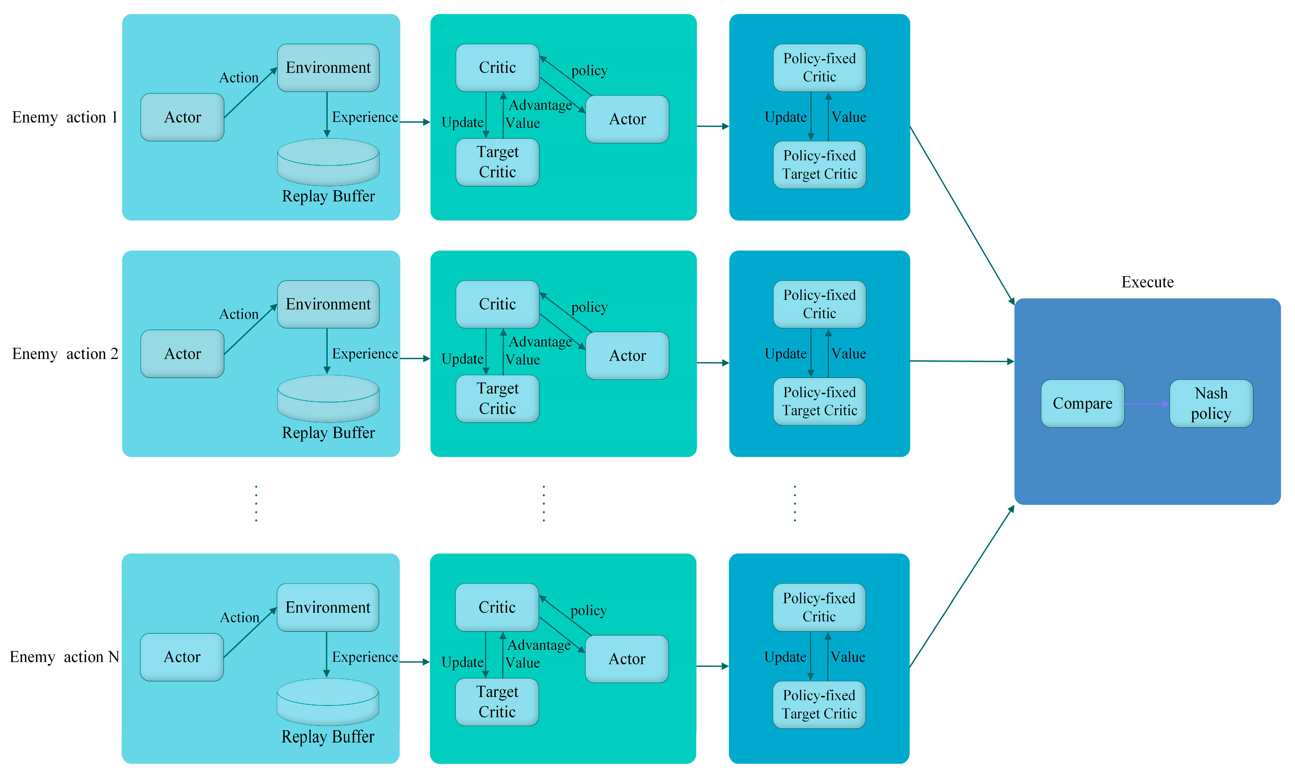
After decomposition, the model-solving algorithm is divided into two stages: The first stage involves employing parallel training with multiple threads. In each thread corresponding to μ , s d ( s ) V ( π , μ ) ( s ) is used as the indicator function, c, and the policy function is fitted using neural networks [28]. This process is combined with the TD algorithm for parameter updates [29], resulting in determination of the optimal policy for each strategy within the swarm. The comparison decision is made in the second stage of the algorithm. For any given state s , we input it into each thread’s value-function network to obtain the predicted weighted cumulative reward. We then compare these rewards to find the policy corresponding to the minimum value, which is the MPE policy of the MG. We then execute the algorithm according to this policy to effectively complete the UAVs-CJ-related tasks.
During the process, the following four operations are performed: reducing the algorithm thread count using the approach from reference [15], introducing the advantage actor–critic algorithm [30] into Equation (17) to decrease training data variance and enhance convergence stability, employing the off-policy paradigm [31] for exploration using the behavioral policies β to improve data utilization efficiency, and introducing target networks to alleviate overfitting.
The algorithm flowchart and pseudocode are in Figure 2 and Algorithm 2:
Algorithm 2: M2AC Learning Algorithm
Input: Behavior policy β ( | s ) , discount factor γ , exploration factor ε t , sample number m , target update steps T and learning rate α , soft update parameter τ
1: Initialization: neural actor network parameter under N enemy action θ 1 , θ 2 , , θ N , neural critic network parameter under N enemy action ϕ 1 , ϕ 2 , , ϕ N and ϕ 1 t a r g e t , ϕ 2 t a r g e t , , ϕ N t a r g e t , experience memory D 1 , D 2 , , D N , t = 0 and get initial state s 0
2: For t = 0, 1, … do
3: For n = 0, 1, … do
4: Build thread
5: Choose action according to behavior policy β
6: Choose opponent action b t (which are fixed in each thread)
7: Execute a t and b t and get r t + 1 and s t + 1 and store ( s t , a t , b t , r t + 1 , s t + 1 ) in D n
8: Sample m batches ( b a t c h 1 , b a t c h 2 , , b a t c h m ) from D n
9: δ k = r k + 1 + γ V ( s k + 1 | ϕ n t a r g e t ) V ( s k | ϕ n )
10: θ n = θ n + α θ δ k θ n ln π ( a k | s k , θ n ) π ( a k | s k , θ n ) / β ( a k | s k )
11: ϕ n = ϕ n + α ϕ δ k θ n V ( s k | ϕ n ) π ( a k | s k , θ n ) β ( a k | s k )
12: ϕ n t a r g e t = τ ϕ 1 + ( 1 τ ) ϕ n t a r g e t
13: end for
14: end for
15: Train Critic Network ϕ π 1 , ϕ π 2 , , ϕ π N
Output: minimax police π * = min π ( V ( ϕ π 1 , ϕ π 2 , , ϕ π N ) )
It can be observed that, compared to the M2DQN algorithm, the M2AC algorithm increases the number of networks and parallel operations at the cost of avoiding linear programming, which addresses the timeliness constraints.

4. Simulation and Analysis

This section verifies the effectiveness and timeliness of the UAVs-CJ intelligent decision-making algorithm based on the M2AC algorithm.

4.1. Analysis of Algorithm Effectiveness

This subsection comprehensively analyzes the effectiveness of the algorithm from three perspectives: the effectiveness of the jamming policy, the effectiveness of the value function prediction, and the effectiveness of the decision results. During the simulation experiments, the number of UAVs in swarm Red and swarm Blue was set to three, and their initial positions, final positions, UAV movement speed, and UAV size are listed in Table 1. We set the network with two hidden layers, the policy network’s output layer uses the softmax function, and we employed the Adam optimizer with a learning rate of 0.0005. The training batch size was 32, and the discount factor γ was 0.99.
Regarding the setting of node weights ω , we found that as long as the value of the cluster head node is greater than the other nodes, the final result remains unchanged. Therefore, we did not list and analyze this parameter.

4.2. Effectiveness of Jamming Strategies

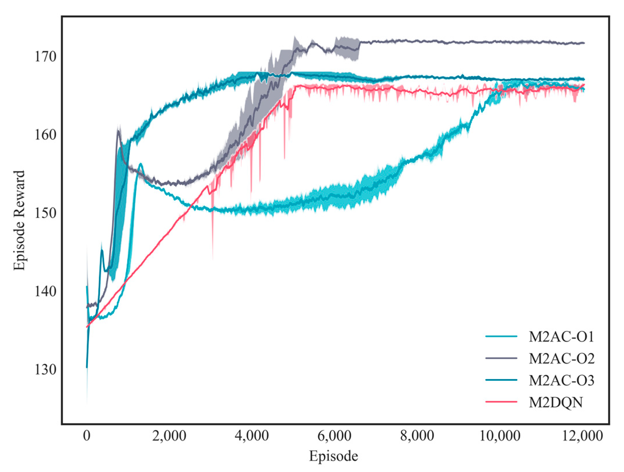
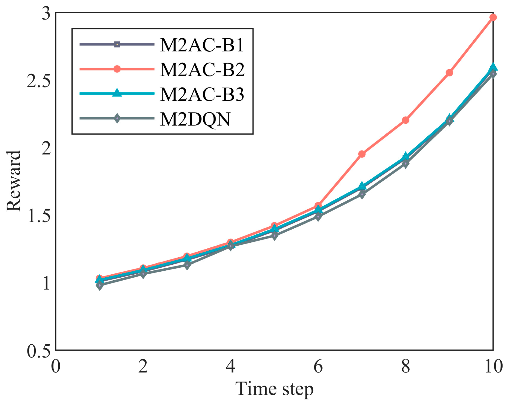
A jamming policy is obtained from the converged policy network during the multithreaded parallel training phase of the algorithm. In the 3v3-scale UAVs-CJ simulation scenario, the UAV swarm generally adopts a single-cluster structure for communication networking, selecting the node with the best communication status as the cluster head node for communication. Here, the cluster action corresponds to three optional communication structures, and the algorithm has three threads. The parallel training results for each thread are shown in Figure 3, which synchronously displays the training results of the M2DQN algorithm. The solid line represents the average results of the two experiments, while the shaded areas on both sides represent the training results corresponding to the two repeated experiments.
Figure 3 shows that the training of each thread in the M2AC algorithm achieves convergence. The final convergence results of each thread are slightly different owing to the different actions of swarm Blue. The M2DQN algorithm seeks the minimum value under various actions of swarm Blue. The convergence value should be the minimum among the four curves. However, it is difficult to achieve 100% of the theoretically optimal value in practice. Therefore, there is a slight error, but it still satisfies the trend of the M2DQN algorithm converging to the minimum value.
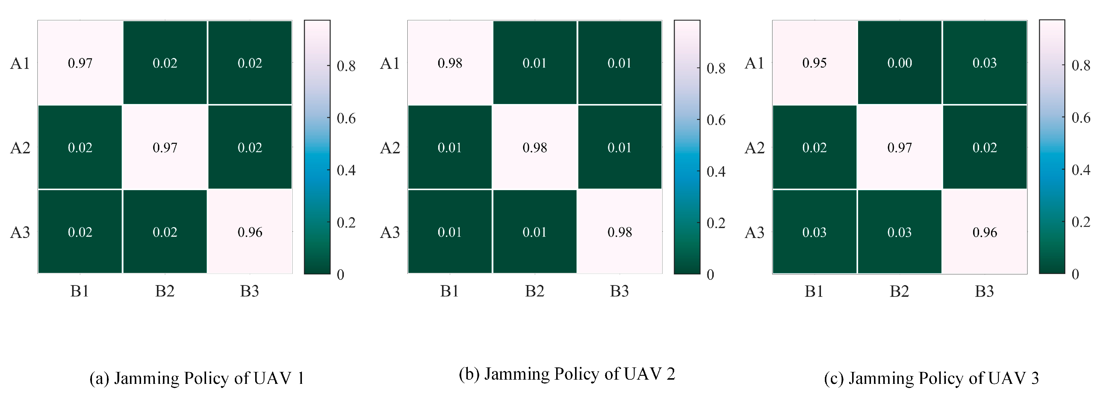
Based on the convergence achieved by the M2AC algorithm, the jamming policies were output by the converged policy network (Figure 4). Figure 4a–c use heatmaps to display the jamming policies of each UAV in swarm Red. From Figure 4, it can be observed that when swarm Blue’s action is B1 (with the first UAV in the swarm as the cluster head), the probability of each UAV in swarm Red jamming with its first UAV—that is, the cluster head—is considerably greater than the probability of jamming with other nodes. This jamming policy is logical because the cluster head plays a central command role in the cluster, and jamming with it can effectively weaken the operational efficiency of swarm Blue compared to jamming with other UAVs. In Figure 4b,c, when swarm Blue’s action is B2 or B3, swarm Red jams significantly with its second and third UAVs, respectively. The targeted interfered nodes are the corresponding cluster heads under the respective actions.
Combining the results displayed in Figure 3 and Figure 4, we can observe that the jamming policies obtained by the convergence of the M2AC algorithm tend to jam with the cluster head of swarm Blue. This strategy can lead to higher rewards, which is consistent with common sense, indicating that the jamming policy is effective.

4.3. Effectiveness of Value Function Prediction

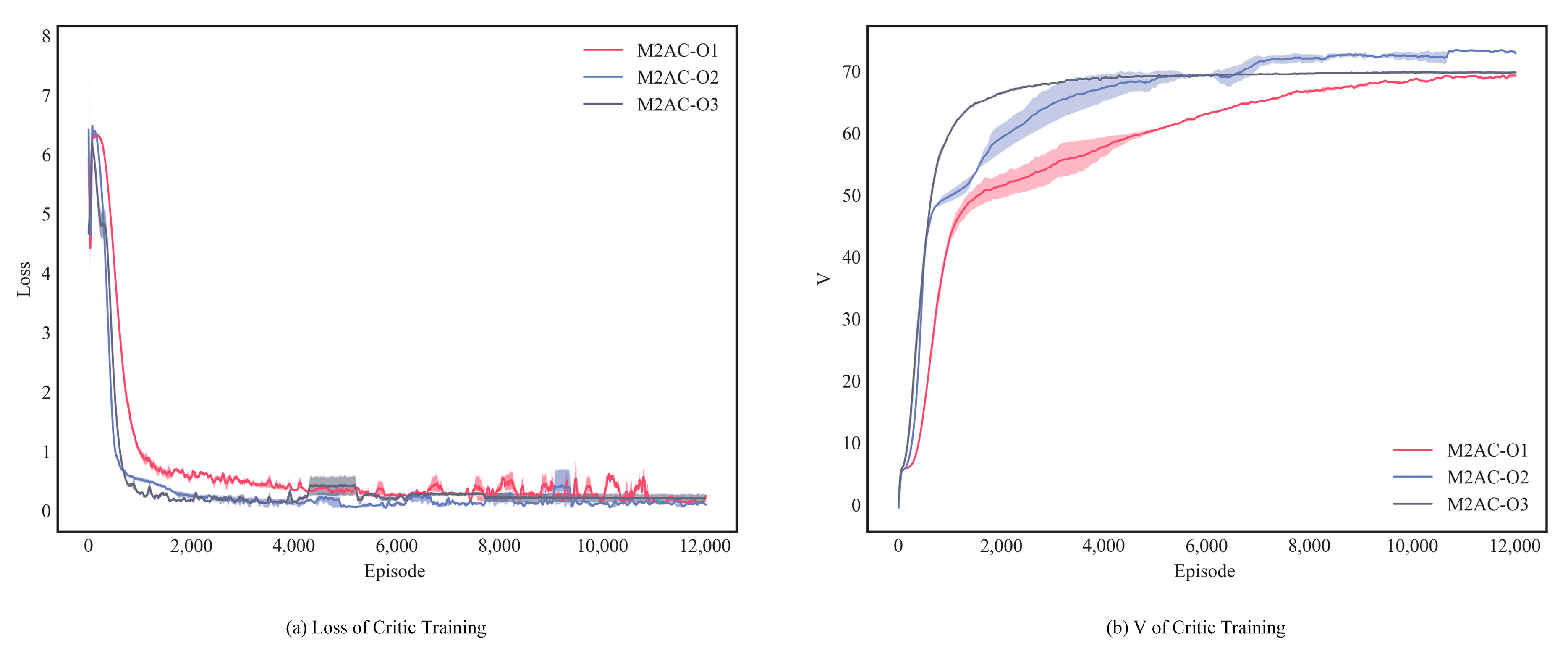
The value function was utilized to predict the weighted cumulative rewards of jamming policies, obtained from the converged critic network during the multithreaded parallel training phase of the algorithm. Figure 5 illustrates the training results of the critic network for each thread. Figure 5a shows the variation in the critic network’s loss under each thread, whereas the change in network outputs is depicted in Figure 5b, where the solid and dashed lines have the same meaning as in Figure 3. The loss represents the difference between the output value and the target value for fitting, with smaller values indicating a closer alignment between the network output and target values. It can be observed that the loss values under all three threads tend to approach zero, whereas the network outputs also tend to stabilize, demonstrating the convergence of the critic network.
Next, the output values of the converged critic network were analyzed. The critic network’s predictions regarding the weighted cumulative rewards of the jamming policies are shown in Figure 6, where the solid lines represent the actual weighted cumulative rewards under the three threads, whereas the circles indicate the output values of the critic network, with error bars showing the relative magnitude of the differences between the output and actual values. The output values of the critic network effectively fit the real cumulative rewards in a relatively stable manner, indicating that the predictions of the value function are effective.

4.4. Effectiveness of the Decision Results

Through multithreaded parallel training, we obtained converged policy and critic networks. During the decision-making phase, we utilized the output values of these networks to derive the final decision. To validate the effectiveness of the decision, we synchronously relied on the M2DQN algorithm for decision-making (Figure 7). The three curves corresponding to M2AC represent the returns obtained by executing the policy networks for each thread, with the minimum value being the final decision. The curve corresponding to M2DQN represents the returns after executing the MPE policy. We can observe that the minimum values of the three curves of M2AC are close to the curve corresponding to the M2DQN algorithm, indicating that the returns obtained by M2AC are nearly identical to those of the M2DQN algorithm; that is, the decision results are almost the same as the MPE policy, demonstrating the effectiveness of the final decision results.

4.5. Decision-Making Effectiveness in Scenarios Involving UAV Swarms of Different Scales

To verify the effectiveness of the M2AC algorithm in scenarios involving UAV swarms of different scales, an effectiveness analysis experiment was conducted for 4v4 and 5v5 scenarios. The UAV movement speed and size remained consistent with those in the 3v3 scenario, as shown in Table 2 and Table 3 for the initial and final positions.
The decision results are shown in Figure 8. Similar to Figure 7, the minimum returns of each thread in M2AC are nearly identical to the returns obtained from the MPE policy of the M2DQN algorithm. In the case of 5v5, there is a certain increase in randomness compared to 3v3, which is due to differences in the scenario settings. Although at some moments the minimum value of M2AC is lower than that of the MPE policy, overall, it still follows the trend of being close to the MPE policy. This demonstrates that the decision results of the M2AC algorithm remain effective in the 4v4 and 5v5 scenarios.
In summary, based on the above analysis, we can observe that in the UAVs-CJ scenario, the jamming policy and value function prediction of the M2AC algorithm align with real-world situations. The decision results obtained are consistent with the MPE policy, indicating that the algorithm can effectively make intelligent decisions in the UAVs-CJ scenario.

4.6. Analysis of Algorithm Timeliness

This section provides a comprehensive analysis of the timeliness of the algorithm from the perspectives of training and decision-making. Compared to the effectiveness analysis, the timeliness analysis adds the MAQL algorithm [32] as a comparative algorithm.
The simulation environment included an Intel(R) Xeon(R) Gold 5218 CPU @ 2.30 GHz processor and 16 GB of memory. Simulation experiments for the proposed approach were carried out using Python. First, the training’s timeliness was analyzed. During the training phase, the M2DQN algorithm’s linear programming operations were implemented using the faster running rates of the highs-ds and highs-ipm solving methods in the Linprog toolbox. The training times of the M2AC and comparative algorithms for different UAV swarm sizes are listed in Table 4, with the same configuration, which shows that even when using the faster highs-ds solving method to implement the M2DQN and MAQL algorithms, the training times were significantly longer than those of the M2AC algorithm across all three drone swarm sizes, indicating that M2AC can enhance training’s timeliness.
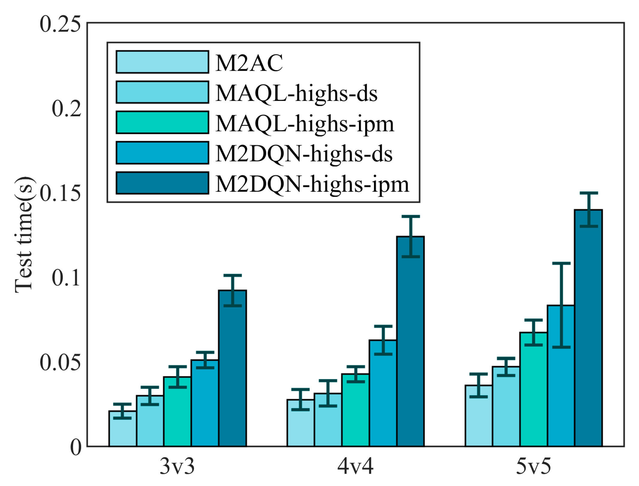
Next, an analysis of decision-making timeliness was conducted. Figure 9 illustrates the decision-making times of the M2AC and comparative algorithms for different UAV swarm sizes, while maintaining the same configuration. The three sets of bar graphs in Figure 9 represent the average decision-making time, with the error bar lengths indicating the variance in the decision-making duration. From the results displayed in Figure 9, it can be observed that M2AC demonstrates higher decision-making timeliness compared to the comparative algorithms.
Combining the analysis of training and decision-making timeliness, the M2AC algorithm proposed in this paper demonstrates stronger timeliness than the comparative algorithms. Building upon the effectiveness analysis of the algorithm in Section 4.1, this section experimentally demonstrates that, under conditions where the M2AC algorithm effectively acquires the MPE strategy, it significantly improves timeliness, thus effectively enhancing decision-making efficiency in the UAVs-CJ scenario.

5. Future Research Directions

On the basis of effectively improving timeliness, the proposed algorithm has several main limitations, which also serve as primary directions for future research. Firstly, there is a limitation on the number of UAVs in the swarms. The algorithm in this paper adopts a multithreaded parallel training paradigm, which to some extent restricts the scale of the swarms. While it can be used for intelligent decision-making in single-cluster scenarios such as 3, 4, and 5 in simulations, increasing the number of threads will lead to increased algorithm complexity, making it difficult to meet the intelligent decision-making needs of multi-cluster UAV swarms; this will be the focus of our next research steps. Secondly, there are hardware limitations. The algorithm was only tested in a software environment; future research is needed on its actual effects on dedicated simulation software and hardware [33,34]. Thirdly, there are spatial limitations. The algorithm was tested in a two-dimensional space; testing in three-dimensional space with increased spatial freedom is also part of our planned future work.

6. Conclusions

This study proposes an intelligent decision-making algorithm based on M2AC to enhance the decision efficiency in high real-time and dynamic UAVs-CJ scenarios. The algorithm models the UAVs-CJ intelligent decision problem as an MG model, converting the decision problem into corresponding mathematical problems. To avoid linear programming operations in value-based algorithms, it directly constructs a policy network, defines the corresponding objective function, and designs a policy network indicator function. Based on this, a multithreaded parallel training–contrast decision approach is adopted to update the policy network and increase the network quantity to achieve faster decision speeds. Through comparative experiments, the M2AC-based algorithm significantly increased the training and decision rates when obtaining the same MPE strategy, providing guidance for improving the performance of UAVs-CJ intelligent decision algorithms.

Author Contributions

Conceptualization, R.H.; methodology, R.H.; writing—original draft preparation, R.H. and Z.T.; writing—review and editing, R.H., D.W., T.H., Z.T., S.Y. and Z.X. All authors have read and agreed to the published version of the manuscript.

Funding

This research was funded by the National Natural Science Foundation of China, grant number 42201472.

Data Availability Statement

The original contributions presented in the study are included in the article, further inquiries can be directed to the corresponding author/s.

DURC Statement

The current research is limited to unmanned intelligent combat, which is beneficial for addressing the challenges of UAV swarms and does not pose a threat to public health or national security. The authors acknowledge the dual-use potential of the research involving unmanned intelligent combat and confirm that all necessary precautions have been taken to prevent potential misuse. As an ethical responsibility, authors strictly adhered to the relevant national and international laws concerning DURC. The authors advocate for responsible deployment, ethical considerations, regulatory compliance, and transparent reporting to mitigate misuse risks and foster beneficial outcomes.

Conflicts of Interest

The authors declare no conflicts of interest.

Appendix A

θ V ( π , μ ) ( s ) = θ [ b μ ( b | s ) a π ( a | s , θ ) Q ( π , μ ) ( s , a , b ) ] = b μ ( b | s ) θ [ a π ( a | s , θ ) Q ( π , μ ) ( s , a , b ) ] = b μ ( b | s ) a [ θ π ( a | s , θ ) Q ( π , μ ) ( s , a , b ) + π ( a | s , θ ) θ Q ( π , μ ) ( s , a , b ) ]
According to the Bellman equation, we can obtain Q ( π , μ ) ( s , a , b ) = R ( s , a , b ) + γ s p s V ( π , μ ) ( s ) ; therefore, we can obtain θ Q ( π , μ ) ( s , a , b ) = γ s p s θ V ( π , μ ) ( s ) . Substituting Equation (A1) in the equation, we obtain
θ V ( π , μ ) ( s ) = b μ ( b | s ) { a θ π ( a | s , θ ) Q ( π , μ ) ( s , a , b ) + γ a π ( a | s , θ ) s p s θ V ( π , μ ) ( s ) }
Let U ( s ) = b μ ( b | s ) a θ π ( a | s , θ ) Q ( π , μ ) ( s , a , b ) , where [ p ( π , μ ) ] s s is the probability of transitioning from a certain state s to state s under the current policy. Based on this, Equation (A2) can be written in matrix form under discrete states:
θ V ( π , μ ) ( s ) = U ( s ) + γ P π θ V ( π , μ ) ( s )
Further simplifying this, we have θ V ( π , μ ) = U + γ P π θ V ( π , μ ) ; consequently, θ V ( π , μ ) = ( I n γ P π ) 1 U , where I n is the n -dimensional identity matrix, and n is the number of states.
Substituting Equation (A2) back in, we have
θ V ( π , μ ) ( s ) = s [ ( I n γ P ( π , μ ) ) 1 ] s s b μ ( b | s ) a θ π ( a | s , θ ) Q ( π , μ ) ( s , a , b )
Rewriting [ ( I n γ P ( π , μ ) ) 1 ] s s as P ( π , μ ) ( s | s ) , we have
θ V ( π , μ ) ( s ) = s P ( π , μ ) ( s | s ) b μ ( b | s ) a θ π ( a | s , θ ) Q ( π , μ ) ( s , a , b )
where P ( π , μ ) ( s | s ) represents the discounted probability sum of transitioning from s to s through any number of timesteps under policy pair P ( π , μ ) ( s | s ) .

References

  1. Wang, B.; Li, S.; Gao, X.; Xie, T. UAV swarm confrontation using hierarchical multiagent reinforcement learning. Int. J. Aerosp. Eng. 2021, 2021, 360116. [Google Scholar] [CrossRef]
  2. Ji, X.; Zhang, W.; Xiang, F.; Yuan, W.; Chen, J. A swarm confrontation method based on Lanchester law and Nash equilibrium. Electronics 2022, 11, 896. [Google Scholar] [CrossRef]
  3. Mo, Z.; Sun, H.-w.; Wang, L.; Yu, S.-z.; Meng, X.-y.; Li, D. Research on foreign anti-UAV swarm warfare. Command Control Simul./Zhihui Kongzhi Yu Fangzhen 2023, 45, 24–30. [Google Scholar] [CrossRef]
  4. Williams, H.P. Model Building in Mathematical Programming; John Wiley & Sons: Hoboken, NJ, USA, 2013. [Google Scholar]
  5. Xing, D.X.; Zhen, Z.; Gong, H. Offense–defense confrontation decision making for dynamic UAV swarm versus UAV swarm. Proc. Inst. Mech. Eng. G 2019, 233, 5689–5702. [Google Scholar] [CrossRef]
  6. Jones, A.J. Game Theory: Mathematical Models of Conflict; Elsevier: Amsterdam, The Netherlands, 2000. [Google Scholar]
  7. Li, S.-Y.; Chen, M.; Wang, Y.; Wu, Q. Air combat decision-making of multiple UCAVs based on constraint strategy games. Def. Technol. 2022, 18, 368–383. [Google Scholar] [CrossRef]
  8. Ma, Y.; Wang, G.; Hu, X.; Luo, H.; Lei, X. Cooperative occupancy decision making of Multi-UAV in Beyond-Visual-Range air combat: A game theory approach. IEEE Access 2019, 8, 11624–11634. [Google Scholar] [CrossRef]
  9. Puterman, M.L. Markov decision processes. Handb. Oper. Res. Manag. Sci. 1990, 2, 331–434. [Google Scholar]
  10. Wang, B.; Li, S.; Gao, X.; Xie, T. Weighted mean field reinforcement learning for large-scale UAV swarm confrontation. Appl. Intell. 2023, 53, 5274–5289. [Google Scholar] [CrossRef]
  11. Fernando, X.; Gupta, A. Analysis of unmanned aerial vehicle-assisted cellular vehicle-to-everything communication using markovian game in a federated learning environment. Drones 2024, 8, 238. [Google Scholar] [CrossRef]
  12. Papoudakis, G.; Christianos, F.; Rahman, A.; Albrecht, S.V. Dealing with non-stationarity in multi-agent deep reinforcement learning. arXiv 2019, arXiv:1906.04737v1. [Google Scholar]
  13. Littman, M.L. Markov games as a framework for multi-agent reinforcement learning. In Machine Learning Proceedings 1994; Morgan Kaufmann: Burlington, MA, USA, 1994; pp. 157–163. [Google Scholar]
  14. Mnih, V.; Kavukcuoglu, K.; Silver, D.; Rusu, A.A.; Veness, J.; Bellemare, M.G.; Graves, A.; Riedmiller, M.; Fidjeland, A.K.; Ostrovski, G.; et al. Human-level control through deep reinforcement learning. Nature 2015, 518, 529–533. [Google Scholar] [CrossRef] [PubMed]
  15. Zhu, Y.; Zhao, D. Online minimax Q network learning for two-player zero-sum Markov games. IEEE Trans. Neural Netw. Learn. Syst. 2022, 33, 1228–1241. [Google Scholar] [CrossRef] [PubMed]
  16. Yan, Y.; Li, G.; Chen, Y.; Fan, J. Model-based reinforcement learning for offline zero-sum markov games. Oper. Res. 2024, 1–16. [Google Scholar] [CrossRef]
  17. Zhong, H.; Xiong, W.; Tan, J.; Wang, L.; Zhang, T.; Wang, Z.; Yang, Z. Pessimistic minimax value iteration: Provably efficient equilibrium learning from offline datasets. In Proceedings of the 39th International Conference on Machine Learning, Baltimore, MD, USA, 17–23 July 2022. [Google Scholar]
  18. Nika, A.; Mandal, D.; Singla, A.; Radanovic, G. Corruption-robust offline two-player zero-sum markov games. In Proceedings of the 27th International Conference on Artificial Intelligence and Statistics, Valencia, Spain, 2–4 May 2024. [Google Scholar]
  19. Arulkumaran, K.; Deisenroth, M.P.; Brundage, M.; Bharath, A.A. Deep reinforcement learning: A brief survey. IEEE Signal Process. Mag. 2017, 34, 26–38. [Google Scholar] [CrossRef]
  20. Grondman, I.; Busoniu, L.; Lopes, G.A.D.; Babuska, R. A survey of actor-critic reinforcement learning: Standard and natural policy gradients. IEEE Trans. Syst. Man. Cybern. C (Appl. Rev.) 2012, 42, 1291–1307. [Google Scholar] [CrossRef]
  21. Vakin, S.A.; Shustov, L.N. Principles of Jamming and Electronic Reconnaissance-Volume I; Tech. Rep. FTD-MT-24-115-69; US Air Force: Washington, DC, USA, 1969; Volume AD692642.
  22. Paine, S.; O’Hagan, D.W.; Inggs, M.; Schupbach, C.; Boniger, U. Evaluating the performance of FM-based PCL radar in the presence of jamming. IEEE Trans. Aerosp. Electron. Syst. 2018, 55, 631–643. [Google Scholar] [CrossRef]
  23. Li, Y. Deep reinforcement learning: An overview. arXiv 2017, arXiv:1701.07274. [Google Scholar]
  24. Patek, S.D. Stochastic and Shortest Path Games: Theory and Algorithms. Ph.D. Thesis, Laboratory for Information and Decision Systems, Massachusetts Institute of Technology, Cambridge, MA, USA, 1997. [Google Scholar]
  25. Sutton, R.S.; McAllester, D.; Singh, S.; Mansour, Y. Policy Gradient Methods for Reinforcement Learning with Function Approximation. In Proceedings of the 12th International Conference on Neural Information Processing Systems, Denver, CO, USA, 29 November–4 December 1999; pp. 1057–1063. [Google Scholar]
  26. Amari, S.I. Backpropagation and stochastic gradient descent method. Neurocomputing 1993, 5, 185–196. [Google Scholar] [CrossRef]
  27. Ruppert, D. Efficient Estimations from a Slowly Convergent Robbins-Monro process; Cornell University Operations Research and Industrial Engineering: Ithaca, NY, USA, 1988. [Google Scholar]
  28. Arena, P.; Fortuna, L.; Occhipinti, L.; Xibilia, M.G. Neural Networks for Quaternion-Valued Function Approximation. In Proceedings of the IEEE International Symposium on Circuits and Systems—ISCAS ’94, London, UK, 30 May–2 June 1994. [Google Scholar] [CrossRef]
  29. Van Seijen, H.; Mahmood, A.R.; Pilarski, P.M.; Machado, M.C.; Sutton, R.S. True online temporal-difference learning. J. Mach. Learn. Res. 2015, 17, 5057–5096. [Google Scholar]
  30. Babaeizadeh, M.; Frosio, I.; Tyree, S.; Clemons, J.; Kautz, J. Reinforcement Learning Through Asynchronous Advantage Actor-Critic on a GPU. arXiv 2016, arXiv:1611.06256. [Google Scholar]
  31. Degris, T.; White, M.; Sutton, R.S. Off-policy actor-critic. arXiv 2012, arXiv:1205.4839. [Google Scholar]
  32. Sayin, M.; Zhang, K.; Leslie, D.; Basar, T.; Ozdaglar, A. Decentralized Q-learning in zero-sum Markov games. In Proceedings of the Advances in Neural Information Processing Systems, Virtual, 6–14 December 2021; Volume 34, pp. 18320–18334. [Google Scholar]
  33. Phadke, A.; Medrano, F.A.; Sekharan, C.N.; Chu, T. An analysis of trends in UAV swarm implementations in current research: Simulation versus hardware. Drone Syst. Appl. 2024, 12, 1–10. [Google Scholar] [CrossRef]
  34. Calderón-Arce, C.; Brenes-Torres, J.C.; Solis-Ortega, R. Swarm robotics: Simulators, platforms and applications review. Computation 2022, 10, 80. [Google Scholar] [CrossRef]
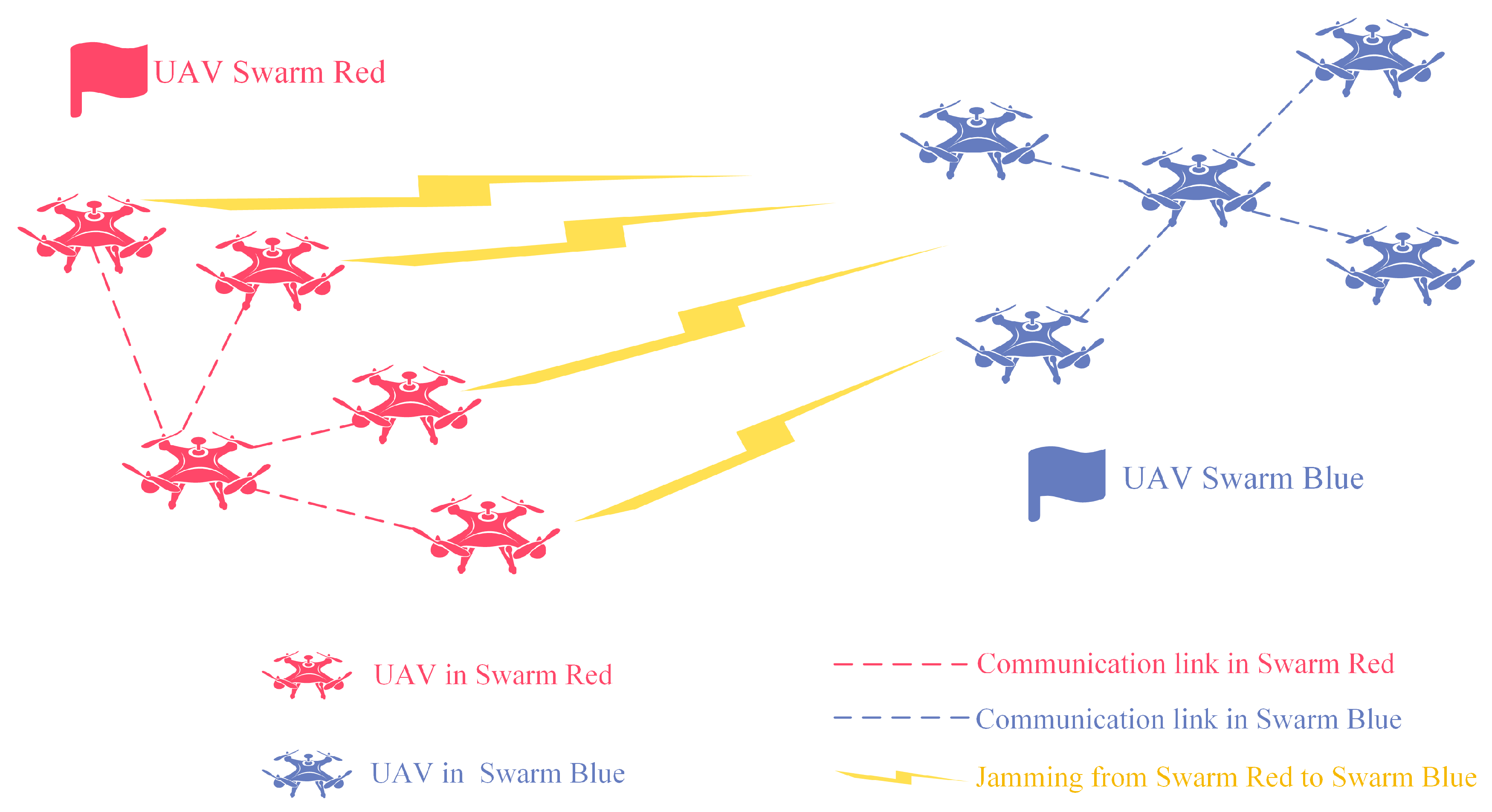
Figure 1. Scene of UAV swarm confrontation jamming.
Drones 08 00338 g001
Figure 2. Flowchart of M2AC algorithm.
Drones 08 00338 g002
Figure 3. Training results of 3v3 UAVs-CJ, where M2AC-B1, M2AC-B2, and M2AC-B3 represent the 1st, 2nd, and 3rd threads, respectively.
Drones 08 00338 g003
Figure 4. Strategy heatmap of 3v3 UAVs-CJ.
Drones 08 00338 g004
Figure 5. Training results of critic, where V represents the output of critic.
Drones 08 00338 g005
Figure 6. Reward forecast of 3v3 UAVs-CJ.
Drones 08 00338 g006
Figure 7. Decision result of 3v3 UAVs-CJ.
Drones 08 00338 g007
Figure 8. Decision results of 4v4 and 5v5 UAVs-CJ.
Drones 08 00338 g008
Figure 9. Comparison diagram of decision times.
Drones 08 00338 g009
Table 1. The 3v3 UAVs-CJ parameter settings.
Initial position of Red (/km)(0.0, 1.0), (0.3, 0.5), (0.0, 0.0)
Initial position of Blue (/km)(15.0, 1.0), (14.7, 0.5), (15.0, 0.0)
Termination position of Red (/km)(5.0, 1.0), (5.3, 0.5), (5.0, 0.0)
Termination position of Blue (/km)(10.0, 1.0), (9.7, 0.5), (10.0, 0.0)
Movement speed of UAV (m/s)5
Table 2. The 4v4 UAVs-CJ parameter settings.
Initial position of Red(0.0, 1.0), (0.3, 0.7), (0.3, 0.3), (0.0, 0.0)
Initial position of Blue(15.0, 1.0), (14.7, 0.7), (14.7, 0.3), (15.0, 0.0)
Termination position of Red(5.0, 1.0), (5.3, 0.7), (5.3, 0.3), (5.0, 0.0)
Termination position of Blue(10.0, 1.0), (9.7, 0.7), (9.7, 0.3), (10.0, 0.0)
Table 3. The 5v5 UAVs-CJ parameter settings.
Initial position of Red(0.0, 1.0), (0.3, 0.7), (0.3, 0.5), (0.3, 0.3), (0.0, 0.0)
Initial position of Blue(15.0, 1.0), (14.7, 0.7), (14.7, 0.5), (14.7, 0.3), (15.0, 0.0)
Termination position of Red(5.0, 1.0), (5.3, 0.7), (5.3, 0.5), (5.3, 0.3), (5.0, 0.0)
Termination position of Blue(10.0, 1.0), (9.7, 0.7), (9.7, 0.5), (9.7, 0.3), (10.0, 0.0)
Table 4. Algorithm training times.
M2ACM2DQN-Highs-dsM2DQN-Highs-ipmMAQL-Highs-dsMAQL-Highs-ipm
3v31 h 50 min16 h 12 min25 h 23 min4 h 25 m6 h 4 m
4v42 h 17 min22 h 1 min34 h 53 min6 h 51 m8 h 57 m
5v52 h 55 min27 h44 h 15 min7 h 22 m10 h 5 m
Disclaimer/Publisher’s Note: The statements, opinions and data contained in all publications are solely those of the individual author(s) and contributor(s) and not of MDPI and/or the editor(s). MDPI and/or the editor(s) disclaim responsibility for any injury to people or property resulting from any ideas, methods, instructions or products referred to in the content.