Author Contributions
Conceptualization, Y.S. (Yuan Shi) and R.L.; methodology, Y.S. (Yuan Shi) and S.L.; software, Y.S. (Yuan Shi); validation, Y.S. (Yuan Shi), R.L. and S.L.; formal analysis, Y.S. (Yuan Shi); investigation, Y.S. (Yuan Shi); resources, R.L. and Y.S. (Yingjing Shi); data curation, Y.S.; writing—original draft preparation, Y.S. (Yuan Shi); writing—review and editing, Y.S. (Yuan Shi), S.L. and R.L.; visualization, Y.S. (Yuan Shi); supervision, R.L. and Y.S. (Yingjing Shi); project administration, R.L. and Y.S. (Yingjing Shi); funding acquisition, R.L. and Y.S. (Yingjing Shi). All authors have read and agreed to the published version of the manuscript.
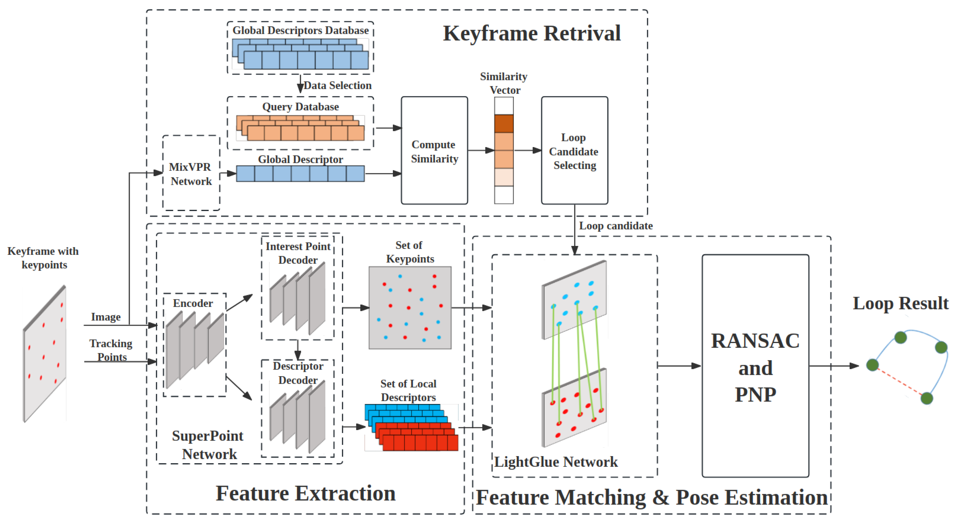
Figure 1.
The pipeline of our loop closure detection approach.
Figure 1.
The pipeline of our loop closure detection approach.
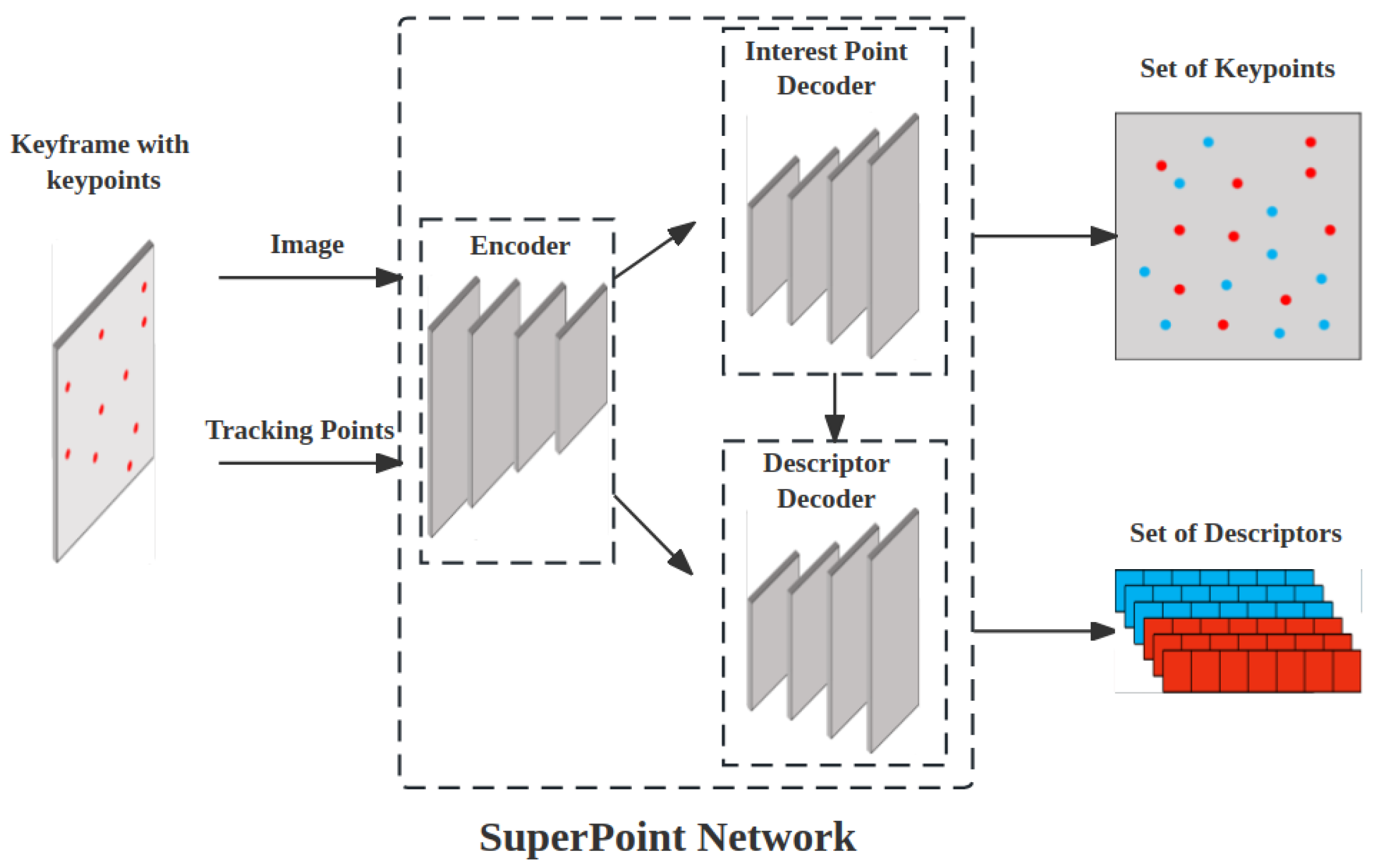
Figure 2.
The pipeline of feature extraction. The red points and vectors represent the feature points and descriptors tracked by the VIO originally, while the blue ones are extracted by SuperPoint.
Figure 2.
The pipeline of feature extraction. The red points and vectors represent the feature points and descriptors tracked by the VIO originally, while the blue ones are extracted by SuperPoint.
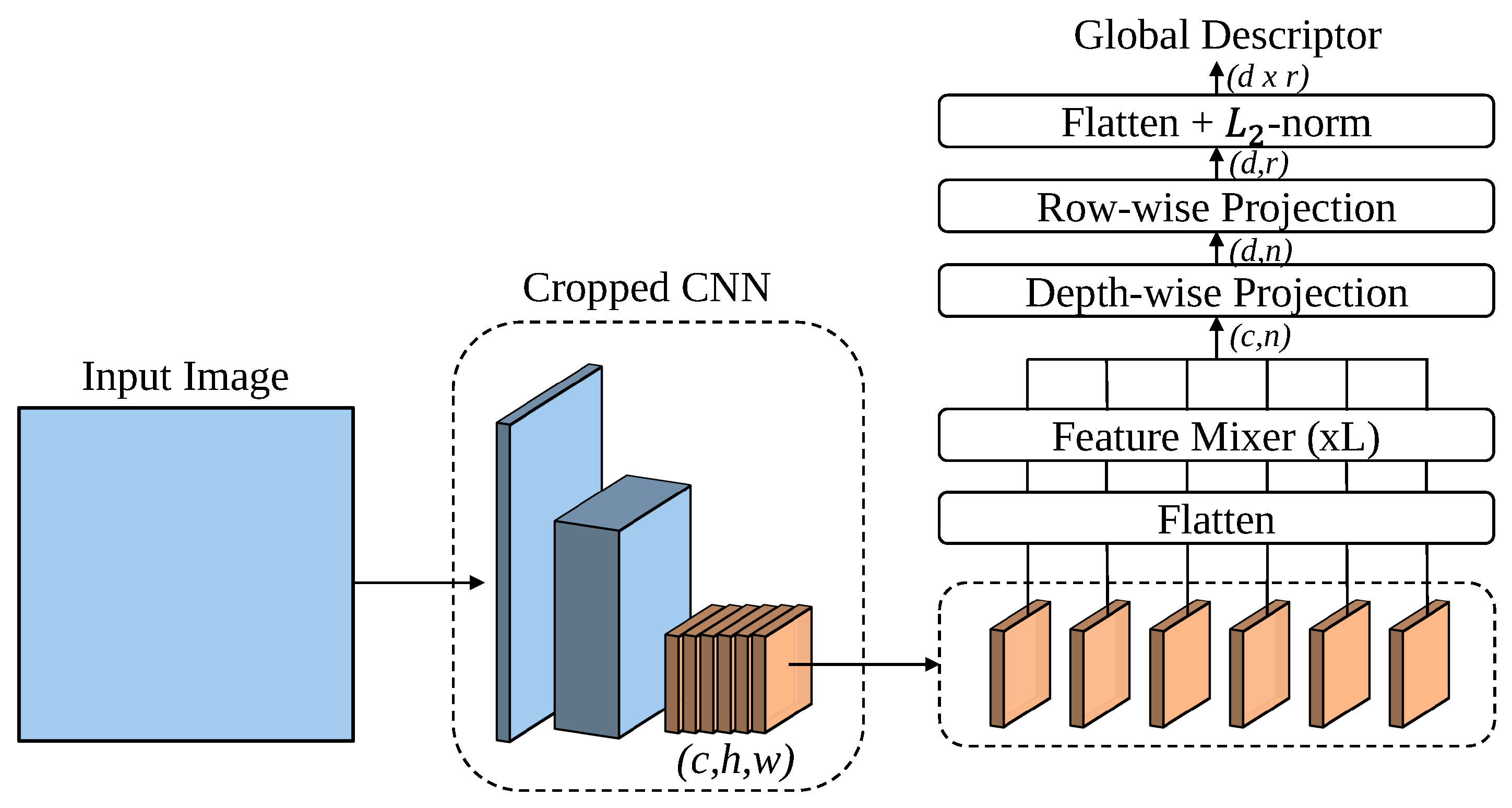
Figure 3.
The overview of the MixVPR network. MixVPR first extracts the holistic feature map from the intermediate layer of the backbone network and, after flattening, inputs it into L Feature Mixers. Then, through projection and flattening operations, it projects the output to a compact representation space, resulting in a low-dimensional descriptor.
Figure 4.
The process of building a global descriptor database and query database Q using MixVPR’s global descriptors.
Figure 4.
The process of building a global descriptor database and query database Q using MixVPR’s global descriptors.
Figure 5.
The process of loop frame retrieval. In the diagram, the darker the grid color of the vector, the higher the similarity of the corresponding vectors in the query database.
Figure 5.
The process of loop frame retrieval. In the diagram, the darker the grid color of the vector, the higher the similarity of the corresponding vectors in the query database.
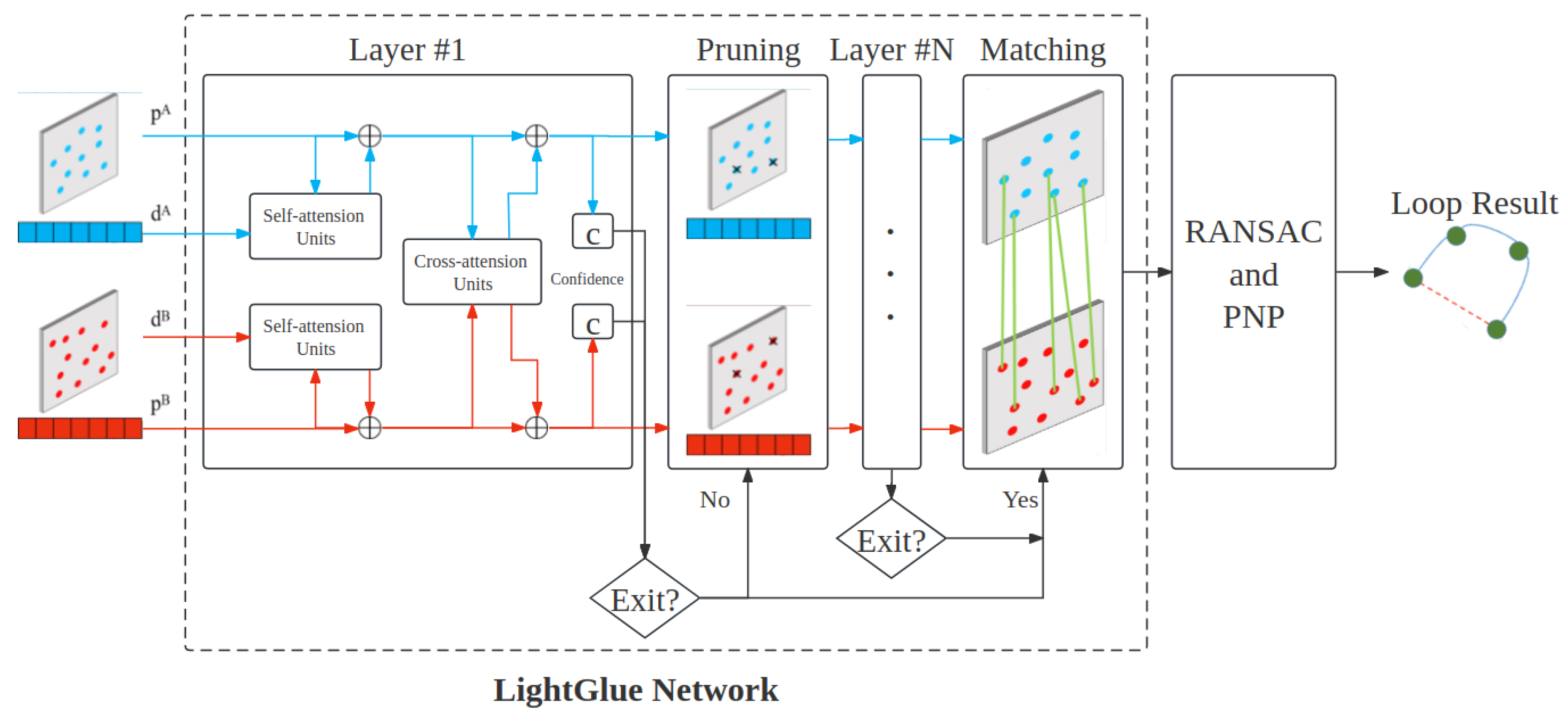
Figure 6.
The process of feature matching and relative pose estimation: represents the feature points of image i, and represents the local descriptors of image i.
Figure 6.
The process of feature matching and relative pose estimation: represents the feature points of image i, and represents the local descriptors of image i.
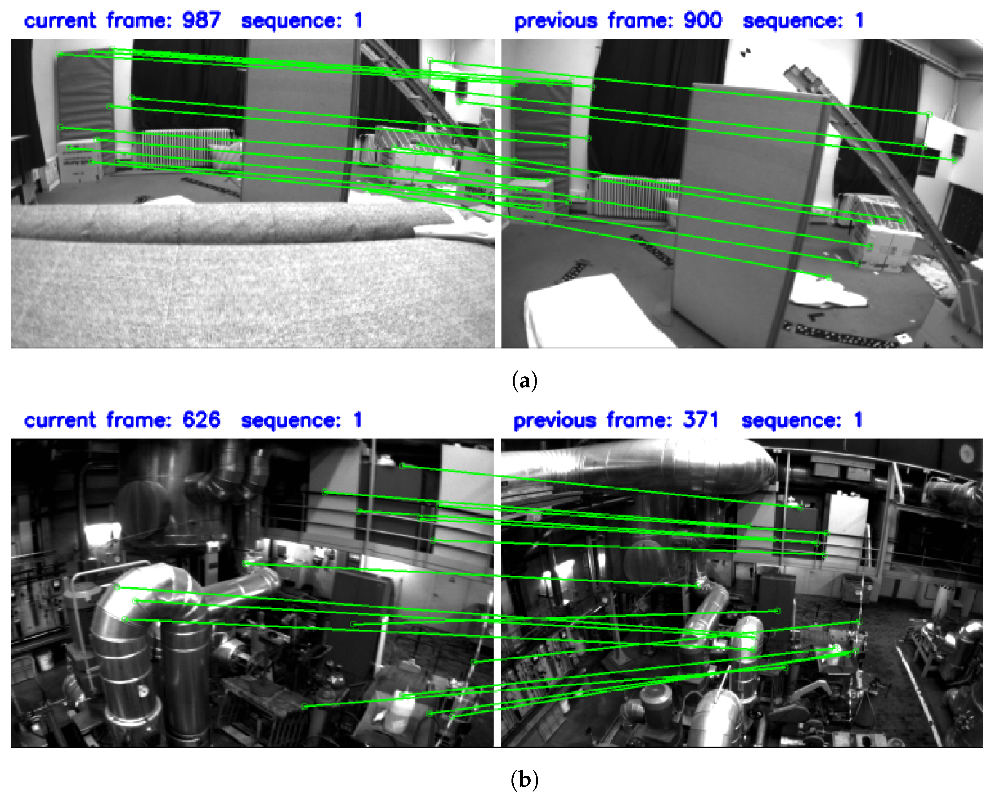
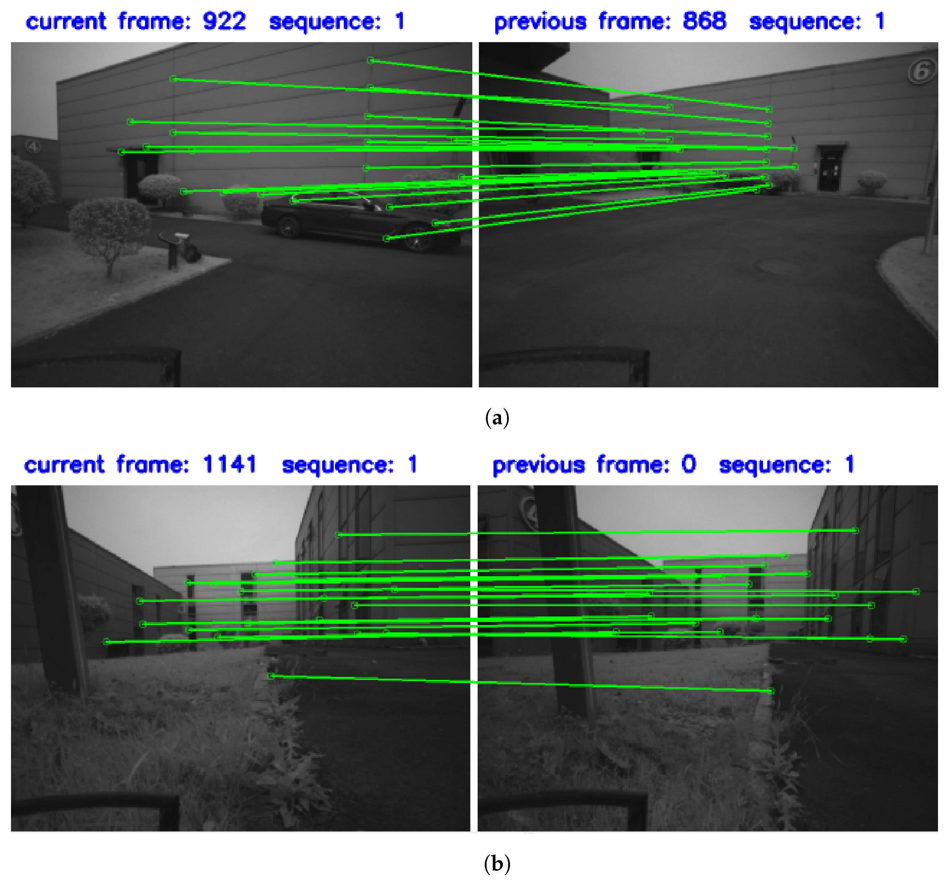
Figure 7.
Matching examples from EuRoC dataset. (a) Match pair before and after takeoff. (b) Match pair with large viewpoint changes.
Figure 7.
Matching examples from EuRoC dataset. (a) Match pair before and after takeoff. (b) Match pair with large viewpoint changes.
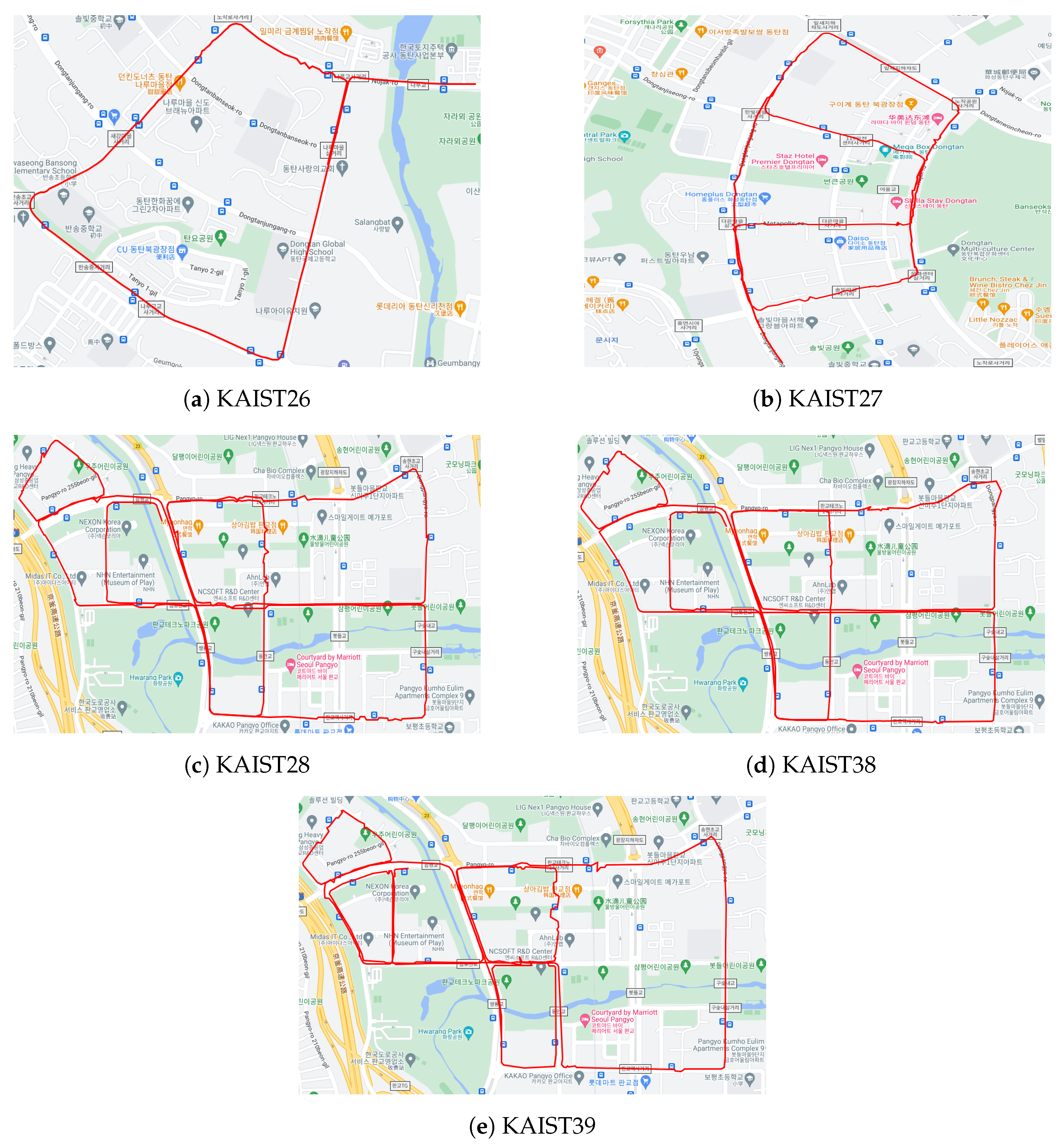
Figure 8.
Sequences from KAIST urban dataset used in this section. (a) Entering the same road only in the last segment of the route with a distance of 4.0 km. (b) Entering the same road twice, entering the opposite direction road once, and the total distance is 5.4 km. (c) Multiple approaches to the same road, multiple approaches to the opposite road, very large scenario, and 11.74 km. (d) The scenario is basically the same as scene 28, but the road conditions and the scene are more complex than scene 28. (e) The scenario is partly the same as scenarios 28 and 38, but the scene has the highest complexity.
Figure 9.
Matching examples from KAIST dataset. (a) Loop closure for long-term tasks. (b) Loop closure in the presence of multiple object occlusions. (c) Loop closure at long distances. (d) Loop closure under strong light conditions.
Figure 9.
Matching examples from KAIST dataset. (a) Loop closure for long-term tasks. (b) Loop closure in the presence of multiple object occlusions. (c) Loop closure at long distances. (d) Loop closure under strong light conditions.
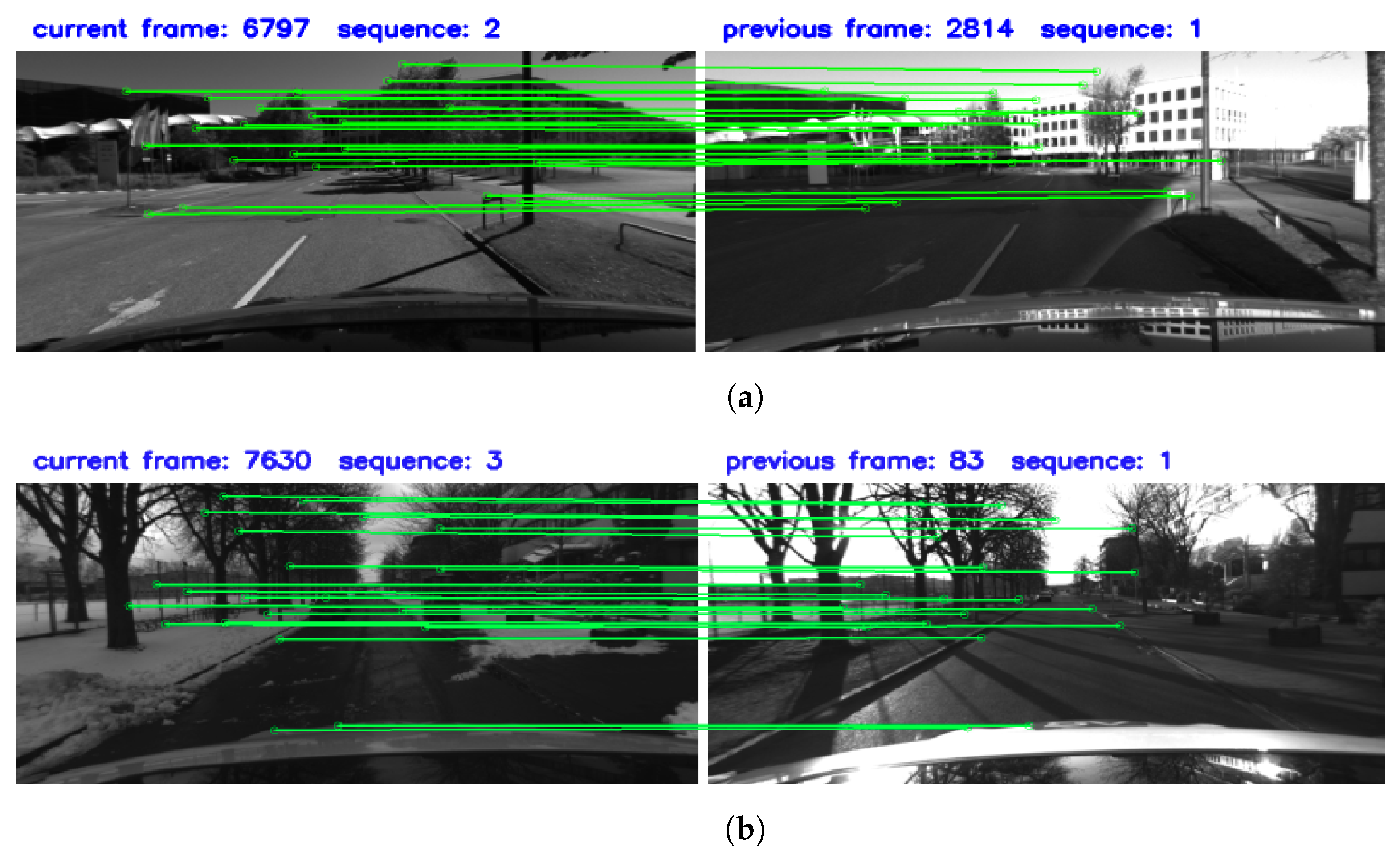
Figure 10.
Matching examples in 4Seasons dataset. (a) Loop closure between spring and summer. (b,c) Loop closure between spring and winter.
Figure 10.
Matching examples in 4Seasons dataset. (a) Loop closure between spring and summer. (b,c) Loop closure between spring and winter.
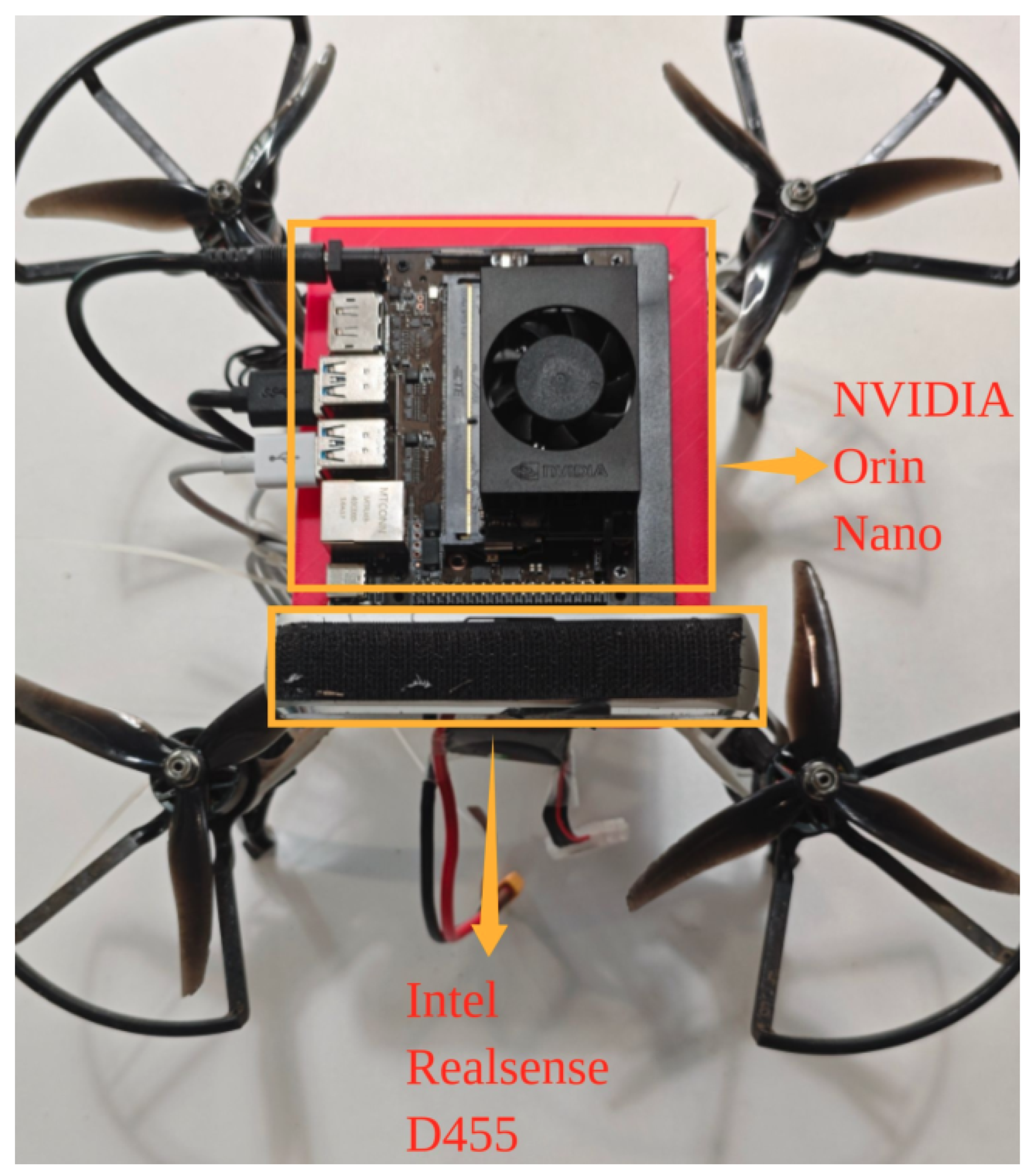
Figure 11.
Self-designed drone equipped with an Intel Realsense D455 camera and NVIDIA Orin Nano platform.
Figure 11.
Self-designed drone equipped with an Intel Realsense D455 camera and NVIDIA Orin Nano platform.
Figure 12.
The overall trajectory diagrams for the simple and difficult sequences. The green trajectory represents the odometry, the red trajectory represents the loop closure, and the blue stars indicate the starting and ending points. (a) The route of a simple sequence. (b) The route of a difficult sequence.
Figure 13.
Experimental result of the simple sequence. The green line represents the odometry trajectory, the red line represents the loop closure trajectory, the blue stars indicate the starting points, and the white stars mark the endpoints of the trajectories. (a) VINS-Loop. (b) SP-LOOP. (c) Ours.
Figure 14.
Experimental results for the difficult sequence. The red line represents the loop closure trajectory, the blue stars indicate the starting points, and the white stars mark the endpoints of the trajectories. (a) VINS-Loop. (b) SP-LOOP. (c) Ours.
Figure 14.
Experimental results for the difficult sequence. The red line represents the loop closure trajectory, the blue stars indicate the starting points, and the white stars mark the endpoints of the trajectories. (a) VINS-Loop. (b) SP-LOOP. (c) Ours.
Figure 15.
Matching examples in real-world experiment. (a) Loop closure at long distances. (b) Loop closure between the starting and ending positions for the simple sequence. (c) Loop closure for long-term tasks. (d) Loop closure between the starting and ending positions for the difficult sequence.
Figure 15.
Matching examples in real-world experiment. (a) Loop closure at long distances. (b) Loop closure between the starting and ending positions for the simple sequence. (c) Loop closure for long-term tasks. (d) Loop closure between the starting and ending positions for the difficult sequence.
Table 1.
Comparison with other approaches in the EuRoC dataset using RMSE (m). The best results are highlighted in bold.
Table 1.
Comparison with other approaches in the EuRoC dataset using RMSE (m). The best results are highlighted in bold.
| Sequence | VINS-VIO | VINS-Loop | SP-LOOP | Ours |
|---|
| V1_01_easy | 0.098 | 0.048 | 0.042 | 0.044 |
| V1_02_medium | 0.098 | 0.055 | 0.034 | 0.050 |
| V1_03_difficult | 0.103 | 0.103 | 0.082 | 0.057 |
| V2_01_easy | 0.127 | 0.053 | 0.038 | 0.059 |
| V2_02_medium | 0.123 | 0.088 | 0.054 | 0.056 |
| V2_03_difficult | 0.345 | 0.085 | 0.10 | 0.075 |
| MH_01_easy | 0.160 | 0.049 | 0.070 | 0.058 |
| MH_02_easy | 0.177 | 0.064 | 0.044 | 0.033 |
| MH_03_medium | 0.315 | 0.065 | 0.068 | 0.057 |
| MH_04_difficult | 0.319 | 0.108 | 0.10 | 0.079 |
| MH_05_difficult | 0.177 | 0.095 | 0.09 | 0.081 |
| Average | 0.186 | 0.074 | 0.066 | 0.059 |
Table 2.
Comparison with other approaches in the KAIST urban dataset using RMSE (m). The best results are highlighted in bold.
Table 2.
Comparison with other approaches in the KAIST urban dataset using RMSE (m). The best results are highlighted in bold.
| Sequence | VINS-VIO | VINS-Loop | SP-LOOP | Ours |
|---|
| urban26 | 14.126 | 11.663 | 14.122 | 5.445 |
| urban27 | 21.359 | 17.655 | 21.204 | 7.256 |
| urban28 | 12.024 | 6.209 | 11.432 | 5.217 |
| urban38 | 8.879 | 7.833 | 7.356 | 8.119 |
| urban39 | 12.831 | 5.772 | 7.310 | 5.623 |
| Average | 13.844 | 9.826 | 12.285 | 6.332 |
Table 3.
Comparison with other approaches for the 4Seasons dataset using RMSE (m). The best results are highlighted in bold.
Table 3.
Comparison with other approaches for the 4Seasons dataset using RMSE (m). The best results are highlighted in bold.
| Sequence | VINS-VIO | VINS-Loop | Ours |
|---|
| 1_spring _sunny | 88.413 | 49.764 | 20.735 |
| 3_summer _sunny | 73.317 | 34.887 | 16.968 |
| 5_winter_snowy | 57.252 | 16.913 | 19.681 |
| Average | 72.994 | 33.855 | 19.128 |
Table 4.
Comparison with other approaches in the real-world experiment using ATE (m). The best results are highlighted in bold.
Table 4.
Comparison with other approaches in the real-world experiment using ATE (m). The best results are highlighted in bold.
| Sequence | VINS-VIO | VINS-Loop | SP-LOOP | Ours |
|---|
| outdoor_easy | 1.337 | 1.266 | 0.122 | 0.115 |
| outdoor_difficult | 41.745 | 29.807 | 2.681 | 0.473 |
Table 5.
The runtime (ms) for each part of our approach on the desktop.
Table 5.
The runtime (ms) for each part of our approach on the desktop.
| Dataset | Global Feature Extraction | Local Feature Extraction | Keyframe Retrieval | Feature Matching |
|---|
| EuRoC | 1.5 | 6.1 | 0.8 | 4.1 |
| KAIST | 2.3 | 10.3 | 1.7 | 3.8 |
| 4Seasons | 2 | 5.4 | 2.2 | 4.1 |
Table 6.
The time cost (ms) and GPU memory cost (MB) of our approach on the desktop.
Table 6.
The time cost (ms) and GPU memory cost (MB) of our approach on the desktop.
| Total Cost | Dataset |
|---|
| EuRoC | KAIST | 4Seasons |
|---|
| Time cost | 12.5 | 18.1 | 13.7 |
| GPU memory cost | 422 | 600 | 400 |
Table 7.
The runtime (ms) for each part of our approach on the Orin Nano.
Table 7.
The runtime (ms) for each part of our approach on the Orin Nano.
| Dataset | Global Feature Extraction | Local Feature Extraction | Keyframe Retrival | Feature Matching |
|---|
| EuRoC | 8.48 | 53 | 0.7 | 28.3 |
| KAIST | 10.2 | 98.48 | 1.8 | 33.4 |
| 4Seasons | 8.71 | 57.88 | 2.3 | 26.7 |
Table 8.
The time cost (ms) and GPU memory cost (MB) of our approach on the Orin Nano.
Table 8.
The time cost (ms) and GPU memory cost (MB) of our approach on the Orin Nano.
| Total Cost | Dataset |
|---|
| EuRoC | KAIST | 4Seasons |
|---|
| Time cost | 90.48 | 143.88 | 95.59 |
| GPU memory cost | 753 | 824 | 734 |
