Article

Ensemble Learning for Pea Yield Estimation Using Unmanned Aerial Vehicles, Red Green Blue, and Multispectral Imagery

by
Zehao Liu
1,†,
Yishan Ji
1,†,
Xiuxiu Ya
2,
Rong Liu
1,
Zhenxing Liu
2,*,
Xuxiao Zong
1 and
Tao Yang
1,*
1
State Key Laboratory of Crop Gene Resources and Breeding, Institute of Crop Sciences, Chinese Academy of Agricultural Sciences, Haidian District, Beijing 100081, China
2
Tangshan Academy of Agricultural Sciences (TAAS), Tangshan 036001, China
*
Authors to whom correspondence should be addressed.
These authors contributed equally to this work.
Drones 2024, 8(6), 227; https://doi.org/10.3390/drones8060227
Submission received: 24 April 2024 / Revised: 25 May 2024 / Accepted: 28 May 2024 / Published: 29 May 2024
(This article belongs to the Special Issue Advances of UAV in Precision Agriculture)

Abstract

:
Peas are one of the most important cultivated legumes worldwide, for which early yield estimations are helpful for agricultural planning. The unmanned aerial vehicles (UAVs) have become widely used for crop yield estimations, owing to their operational convenience. In this study, three types of sensor data (red green blue [RGB], multispectral [MS], and a fusion of RGB and MS) across five growth stages were applied to estimate pea yield using ensemble learning (EL) and four base learners (Cubist, elastic net [EN], K nearest neighbor [KNN], and random forest [RF]). The results showed the following: (1) the use of fusion data effectively improved the estimation accuracy in all five growth stages compared to the estimations obtained using a single sensor; (2) the mid filling growth stage provided the highest estimation accuracy, with coefficients of determination (R2) reaching up to 0.81, 0.8, 0.58, and 0.77 for the Cubist, EN, KNN, and RF algorithms, respectively; (3) the EL algorithm achieved the best performance in estimating pea yield than base learners; and (4) the different models were satisfactory and applicable for both investigated pea types. These results indicated that the combination of dual-sensor data (RGB + MS) from UAVs and appropriate algorithms can be used to obtain sufficiently accurate pea yield estimations, which could provide valuable insights for agricultural remote sensing research.

1. Introduction

The term “nutrition” mainly refers to monocotyledon crops, such as maize, wheat, and rice. Peas (Pisum sativum L.) are an important dicotyledonous crop with moderate protein and energy [1]. Statistical data from the Food and Agriculture Organization in 2021 indicate a dry pea production of 12.40 million tons in 99 countries and a fresh pea production of 20.52 million tons in 86 countries. Worldwide, China has contributed 11.83% and 55.84% of dry and green peas, respectively [2]. The reduction in arable land in China has exacerbated the conflict between the demand for food and land use policies [3]. A rapid and effective estimation of pea yield at the field scale is therefore critical for making field decisions and trade policy [4].
The traditional methods of measuring crop yield can be categorized into two types. One is ground-based field surveys or expert farmer knowledge to obtain detailed yield data. However, it is labor-consuming and too late for field management. The other is using non-destructive techniques (such as measuring leaf area index and spad values) to observe crop morphological characteristics and estimate the yield. However, this method is subjective and challenging to apply over large areas [5,6].
Satellite data have become increasingly used for crop yield estimation in recent decades. Battude et al. [7] combined the simple regression for yield estimates by using several satellite data to obtain accurate maize yield estimates over large areas. Xie and Huang [8] used MODIS time series data to estimate yields in growing areas by using deep learning methods. However, the application of satellite data in precision agriculture remains limited, owing to the relatively high associated costs, limited flexibility regarding the spatial and temporal resolutions of the data, and the effects of meteorological conditions [9].
With the development of the low-altitude platform and integration of sensors [10], a large number of researchers and breeders have turned their attention to acquire high temporal and spatial resolution images by employing unmanned aerial vehicles (UAVs) [11,12,13]. A growing number of studies in the literature are now using UAV remote sensing images for crop yield estimations. For instance, Peng et al. [14] used leaf area index data collected with a UAV to estimate maize yields, and they obtained high accuracy. Song et al. [15] applied UAV data to generate high-spatial-resolution maps, which were then used to estimate yields. Vega et al. [16] developed a method for estimating sunflower yields using multitemporal images from a UAV system carrying a multispectral sensor (MS) during the growing season. Soybean [17], sorghum [18], barley [19], and cotton [20] yields have also been successfully estimated using UAV remote sensing data. However, despite these advances, scant research attention has been paid to pea yield estimations based on UAV remote sensing images.
Several sensors have been adopted to collect data for estimating crop yield, including red green blue (RGB) cameras [21], MS cameras [22], hyperspectral cameras [23], and lidar [24]. Among them, RGB and MS cameras are the most widely favored, owing to their affordable price, simple operation, and easy transport aboard UAVs. Zhang et al. [25] used RGB images obtained using consumer-grade UAVs to extract the excess green (ExG) color feature, thereby establishing a corn yield estimation model and demonstrating the potential of RGB cameras for yield estimates. Huang et al. [26] estimated the yield of cotton based on the vegetation index ratio (RVI) extracted from an MS camera, achieving good results. Héctor et al. [27] analyzed different vegetation indices, canopy cover, and plant densities using RGB and MS cameras, and applied a neural network model to estimated corn grain yields. Their results showed that RGB and MS cameras can provide a high coefficient of determination (R2) between the estimated and observed yields, thus allowing corn grain yields to be accurately characterized and estimated.
Machine learning methods have become a major trend in agricultural research for supporting yield estimations, and have been successfully applied to many crops. Li et al. [28] applied artificial neural network (ANN), support vector machine (SVM), stepwise multiple regression, and random forest (RF) to estimate wheat yields, which indicated that the ANN model obtained higher accuracy than other models. Ashapure et al. [29] estimated cotton yields through ANN, SVM, and RF models, revealing that the ANN model outperformed both the SVM and RF models. Guo et al. [30] adopted several models to estimation maize yields, and presented the finding that the SVM provided better estimates than other machine learning methods, although machine learning techniques have demonstrated their ability to estimate crop traits. However, relying on a single estimation model may lead to the occurrence of overfitting, especially when dealing with limited training data. In contrast, ensemble learning (EL), which combines multiple learners, typically achieved significantly superior generalization performance compared to a single learner. This has been empirically demonstrated in previous studies on various crops. For example, Ji et al. demonstrated that the use of EL significantly outperforms the use of a single model in estimating faba bean yield performance [31]. The applications of pea yield estimation have not been reported yet.
Considering the above, the aims of this study are to: (1) evaluate the estimation performance of pea yields obtained using UAV-based RGB, MS, and feature-level fusion data (RGB + MS); (2) compare the pea yield estimation accuracy in five growth stages; (3) explore the performance of EL and base learners in estimating pea yield; and (4) explore and compare the applicability of machine learning methods for two different pea types (cold-tolerant and common peas).

2. Materials and Methods

2.1. Test Design and Pea Yield Measurement

In this study, peas were sowed on 15 October 2019 and data were collected in 2020. The research was conducted at the experimental base of the Chinese Academy of Agricultural Sciences in Xinxiang, Henan province (113°45′38″ E, 35°8′10″ N). The annual average temperature and humidity of Xinxiang are 14 °C and 68%, respectively. The annual average rainfall is 656.3 mm. The period from June to September is the wettest, with an average precipitation of 409.7 mm. The test site had 90 plots with dimensions of 8 m2 (4 × 2 m; length × width), and 30 pea varieties (16 cold-tolerant varieties and 14 common varieties) were planted with three replicates (Figure 1).
Prior to sowing, it was important to thoroughly plow and harrow the land to loosen the soil and encourage root development, while also applying compound fertilizer at a rate of 600 kg.ha−1. When planting the seeds, the row planting method with a row spacing of 40 cm and a plant spacing of 10 cm was used, and the seeds were sown at a depth of 5–8 cm. During the growth of peas, insecticides were regularly sprayed every half month after overwintering, and additional fertilizer was administered during the flowering period. It was crucial to manually remove weeds to ensure healthy growth. At maturity (27 May 2020), we harvested plants from each plot separately, and conducted threshing and weighing to obtain yield data. The average yield of each plot was 826 kg.ha−1, with a minimum of 100 kg.ha−1 and a maximum of 1420 kg.ha−1. The phenological stages of cold-tolerant peas and regular peas are consistent, as detailed in Table 1.

2.2. UAV-Based Images Acquisition and Processing

We adopted a quadcopter DJI Matrice 210 (SZ DJI Technology Co., Shenzhen, China) electric UAV as a low-altitude observation platform. Two sensors, a Zenmuse X7 (SZ DJI Technology Co., Shenzhen, China) camera and a Red-Edge MX camera (MicaSense Inc., Seattle, DC, USA), were mounted on the DJI Matrice 210 for simultaneously collecting high-resolution RGB and MS images. Table 2 lists detailed information regarding the sensors. Figure 2 shows the UAV observation platform and two sensors used in this study.
In this study, UAV-based images were collected in five key pea growth periods: branching (7 March 2020), flowering (3 April 2020), podding (14 April 2020), early filling (23 April 2020), and mid filling (30 April 2020). The five flight missions were conducted under cloudless conditions between 11:00 AM and 1:00 PM to minimize any disturbances to the images acquired by the UAV by cloud cover and wind. To obtain high-quality images, all flights were set to a height of 25 m, with 85% forward and 85% side overlap for the RGB and MS cameras. The calibrated reflectance panel collected images both before and after the flights, which were later used for MS image calibration. Ground control points (GCPs) were also selected in the field that remained fixed during the study. A differential global navigation satellite system was used to record the GCP coordinates with millimeter precision.
In this study, the RGB and MS images were stitched using Pix4Dmapper 4.4.12 (Pix4D SA, Lausanne, Switzerland) software following the procedure described here. The RGB/MS images and GCP coordinates were first imported into software, and then the “Ag RGB” and “Ag Multispectral” modules in Pix4Dmapper were selected to stitch the RGB and MS images, respectively. For the MS images, the digital number (DN) values were converted to reflectance values using the previously obtained calibrated reflectance panel images. A digital surface model (DSM), digital terrain model (DTM), and orthomosaic of the test site were then obtained in .tif format.

2.3. RGB and MS Feature Extraction

The RGB images were used to extract the plant height (PH), canopy coverage (CC), texture information, and DN values of each plot. And the MS images were used to extract the reflectance of the five bands and texture information in each plot. All features, except the texture information, were extracted using ArcMap 10.5 (Environmental Systems Research Institute, Inc., Redlands, CA, USA), and the texture information was extracted in ENVI 5.3 (ITT Visual Information Solutions, Boulder, CO, USA). During estimation, input was based on the source of the feature. The input features for the RGB sensor include plant height, coverage, and vegetation indices extracted from the RGB sensor. The input features for the MS sensor consist of vegetation indices extracted from the MS sensor. When performing data fusion, all variables extracted from the RGB and MS sensors are utilized as input features.

2.3.1. RGB Data Extraction

The PH is a critical parameter for evaluating crop growth status, which has been proven to correlate highly with yield [32,33]. The PH derived from the RGB images was therefore used as an important feature for estimating pea yield. The DSM image and DTM image obtained by stitching the Pix4Dmapper 4.4.12 images were imported into ArcMap 10.5 software. Just like Equation (1), using the raster calculator, The crop surface model (CSM) image was obtained by subtracting the DSM image from the DTM image. Finally, the maximum value of each small area in the CSM image represents the PH for later data processing.
C S M = D S M D T M
where C S M is the crop surface model, D S M is digital surface model, and D T M is digital terrain model.
The CC refers to the proportion ratio of crop canopy vertical projection area to the ground surface area of each plot, and can reflect the crop growth status and physiological parameters [34]. Before extracting CC, binary mask maps of each growth period were established to effectively exclude the background. The pixels of peas in each plot were then divided by the total number of pixels in the sampled plot to calculate the CC [35] (Equation (2)).
C a n o p y   c o v e r a g e = P c a n o p y / P t o t a l
where P c a n o p y is the number of canopy pixels of peas and P t o t a l is the total number of pixels.
Texture can reflect the structural and geometric features of a canopy [36]. The single bands of the RGB and MS images containing pea plants were used to extract texture information. The extracting method was using the gray-level co-occurrence matrix (GLCM) in ENVI 5.3 [37]. The sliding window and sliding step were set as 7 × 7 and 2 pixels, respectively. Eight parameters from each plot were obtained for further data processing, including the contrast, correlation, dissimilarity, entropy, homogeneity, mean, second moment, and variance.
Vegetation indices (VIs), as an indicator of the spectral features of a canopy, are commonly adopted to estimate crop traits in agriculture research. In this study, the DN values derived from RGB images were used to construct 12 VIs (Table S1) for estimating pea yield.

2.3.2. MS Data Extraction

The radiometrically calibrated MS images were used to extract the reflectance values of each band. The reflectance derived from MS images were adopted to calculate 18 VIs (Table S2) for estimating pea yield.

2.4. Regression Technology

The EL and four base learners (Cubist, EN, KNN, and RF) were selected for estimating pea yield, which were implemented with the “caret” package in R software (V.4.2.2), and the model hyperparameters were tuned using a grid search and five-fold inner cross validation methods.
The Cubist model was developed using Rule Quest, which is based on Quinlan’s M5 model tree algorithm [38]. This algorithm expresses a piecewise multivariate linear function that estimates the value of a variable from a series of independent variables. The training rules of the Cubist model are simple, effective, and fast, and the input space segmentation is automatically carried out by the algorithm, which can handle problems that contain high-dimensional attributes. The Cubist model has been widely applied for leaf area index [39] and yield estimations [40].
The EN algorithm is a linear regression model based on Lasso and Ridge, and is an improvement of several linear regression methods designed for solving high-dimensional feature selection problems. This algorithm can balance the sparsity and accuracy of a model by adjusting the value of parameter α in the objective function and selecting a subset of highly correlated features [41].
The KNN algorithm is used to assign an average value of other sample attributes to an estimation sample to obtain an estimated result. When making an estimation, the distance between the training and test sets should first be calculated, sorted by distance from small to large, and the attributes of the K known samples closest to the estimation sample should be determined. An estimation is then made according to the established decision rules. The size and distance of K are the main factors that affect the KNN model estimation [42]. The characteristics of this model are easy to understand, require a small amount of calculation, and offer a wide range of use.
The RF algorithm is based on the Bagging algorithm with a decision tree as the basic unit algorithm [43], replacement sampling for generating new training sets, and training to obtain a decision tree. Then, the final result was obtained by integrating the estimations of each decision tree. The RF algorithm is characterized by randomness, does not easily fall into overfitting problems, and has a good anti-noise ability [44].
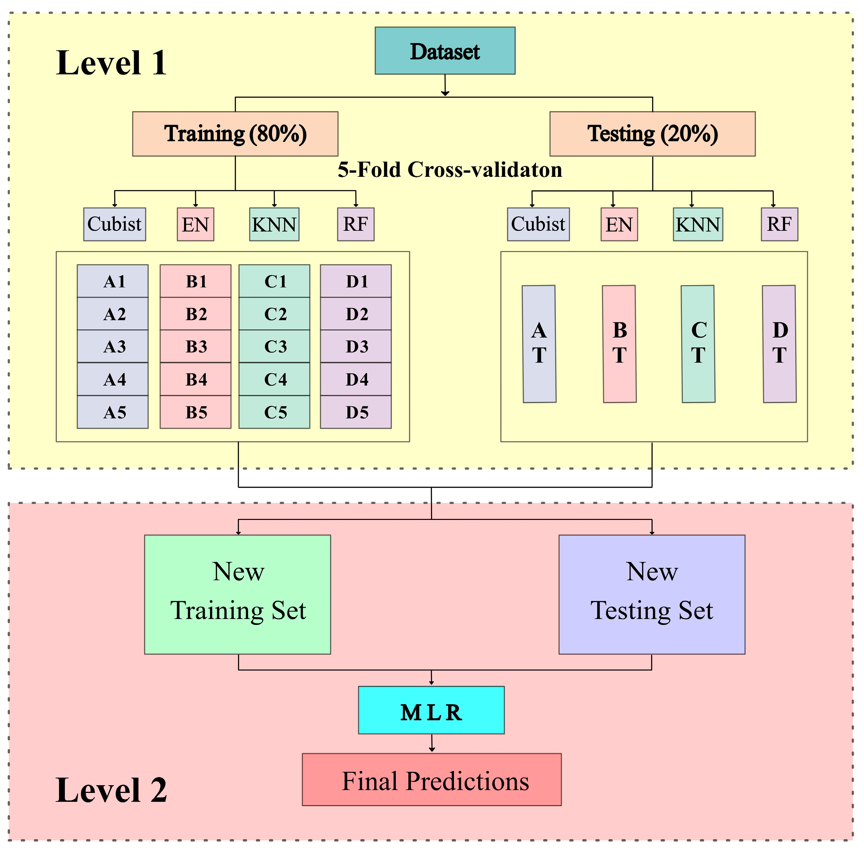
The stacking ensemble learning was first proposed by Wolpert [45]. It is typically a heterogeneous ensemble method that involves training multiple individual learners of different types in parallel. These learners are then combined using a meta-model to generate a final estimation result. As shown in Figure 3, EL consists of two levels. The first layer consists of Cubist, EN, KNN, and RF, where the initial training set is inputted to each base learner using 5-fold cross-validation. In the second level, it consists of combining the estimation results of the base learners into a new matrix, using MLR as the secondary learner, leveraging the predictive abilities of multiple base learners for training, and obtaining the final result.

2.5. Model Performance Evaluation

In order to fairly and completely compare different algorithms in estimating pea yield, we conducted a five-fold cross-validation to test the accuracy of pea yield estimation. The original data were randomly divided into five subsets, with four subsets used as training data and the remaining subset as the test data. This process was repeated five times to ensure that all samples were independently validated. Finally, assessing the model performance using the test set results from five-fold cross-validation.
The R2, the root-mean-square error (RMSE), and the normalized root-mean-square error (NRMSE) were used for evaluating the performance of each algorithms [33].
R 2 = 1 i = 1 n ( X i X i ^ ) 2   /   i = 1 n ( X i X ¯ ) 2
R M S E =   i = 1 n ( X i X i ^ ) 2 / n
N R M S E = R M S E / X ¯
where n is the number of all samples, X i is the measured pea yield of the samples, X i ^ is the estimated pea yield of the samples, and X ¯ denotes the mean of the measured pea yield.

3. Results

3.1. Performance of Sensor Data on Pea Yield

The features extracted from two types of sensors (RGB and MS) and their combination (RGB + MS) were regarded as different datasets for estimating pea yield using Cubist, EN, KNN, and RF models (Table S3). The estimation performances of the single and dual sensors were compared to determine the optimal sensor condition, as indicated by the highest obtained R2 value.
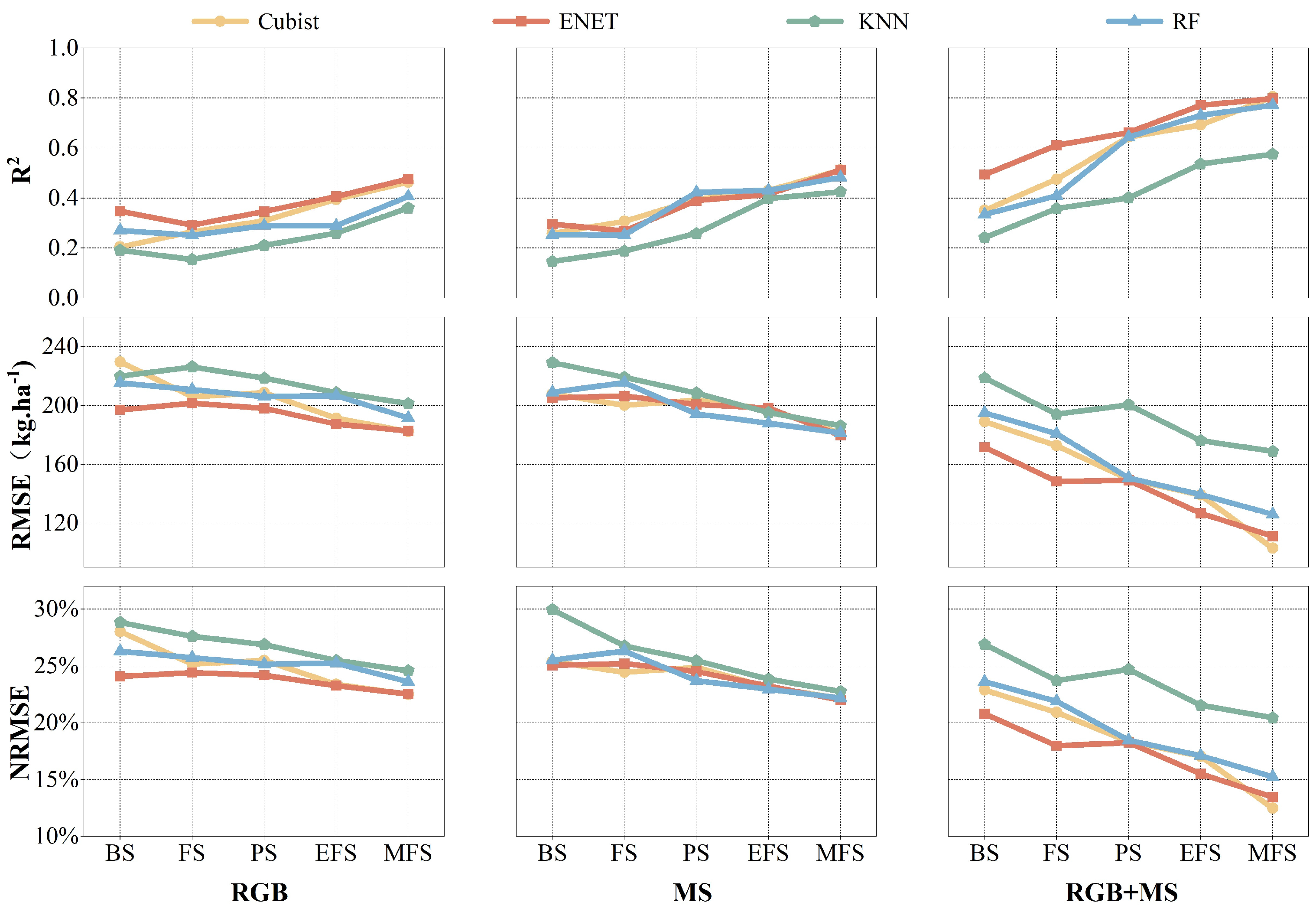
Figure 4 showed the robustness assessment of the pea yield. The MS sensor performed better than the RGB sensor during the flowering, podding, early filling, and mid filling stages, with average R2 values raising by up to 0.25, 0.36, 0.41, and 0.48, respectively. In contrast, the RGB sensor outperformed the MS sensor in the branching stage, with a higher R2 value of up to 0.25.
The accuracy based on the dual sensor (RGB + MS) conditions was found to be superior than that of the single sensors in the five growth stages, with an average accuracy estimation up to 0.34, 0.43, 0.51, 0.58, and 0.74, respectively. The fusion data were therefore more helpful for estimating pea yield.

3.2. Effects of Different Growth Stages on Yield Estimation

To explore the effect of five growth stages on estimating pea yield, the remote sensing data of five growth stages (branching, flowering, podding, early filling, and mid filling stages) were compared using four machine learning algorithms. The average R2 values of the four machine learning algorithms in each growth stage were selected as the result (Figure 5). The mid filling stage yielded the best estimation accuracy based on all sensors, RGB, MS, and their combination with R2 values of 0.43, 0.48, and 0.74, respectively. The next best values were sequentially obtained in the early filling stage (R2 = 0.34, 0.42, and 0.58, respectively), podding stage (R2 = 0.29, 0.37, and 0.51, respectively), and flowering stage (R2 = 0.24, 0.25, and 0.43, respectively), while the branching stage presented the worst estimation accuracy (R2 = 0.25, 0.24, and 0.35, respectively). Figure 6 also showed the R2 values of each algorithm in the five growth stages based on RGB, MS, and RGB + MS. Although the estimation accuracy fluctuated during the flowering and podding stages with some of the algorithms, the overall estimated accuracy showed an increasing trend with growth development.

3.3. Model Performance for Pea Yield Estimation

As indicated in Section 3.1, the fusion of RGB and MS sensors performed better than single sensor in estimating pea yield. Therefore, this section adopted an EL model for estimating pea yield by using the fusion data of RGB and MS, and the estimation performance was compared with four base learners (Table 3).
For base learners, the EN algorithm obtained the best estimation accuracy in the first four growth stages with R2 values of 0.49, 0.61, 0.56, and 0.67, respectively, and NRMSE values of 20.8%, 18.0%, 19.3%, and 16.5%. The Cubist algorithm obtained the best estimation accuracy in the mid filling stage (R2 = 0.805, NRMSE = 12.5%). For the EL algorithm, it achieved the highest R2 values across all five growth stages. Compared to the average performance of the base learners, EL improved by 0.18, 0.19, 0.14, 0.11, and 0.11 for each of the five fertility stages.
In summary, for base learners, the Cubist and EN algorithms both demonstrated better estimation effects for pea yield, while the KNN model was generally poor in this study. Compared with the single model, the EL presented the ability to significantly enhance the estimation accuracy and generalization capability of pea yield.

3.4. Yield Estimation for Different Pea Types

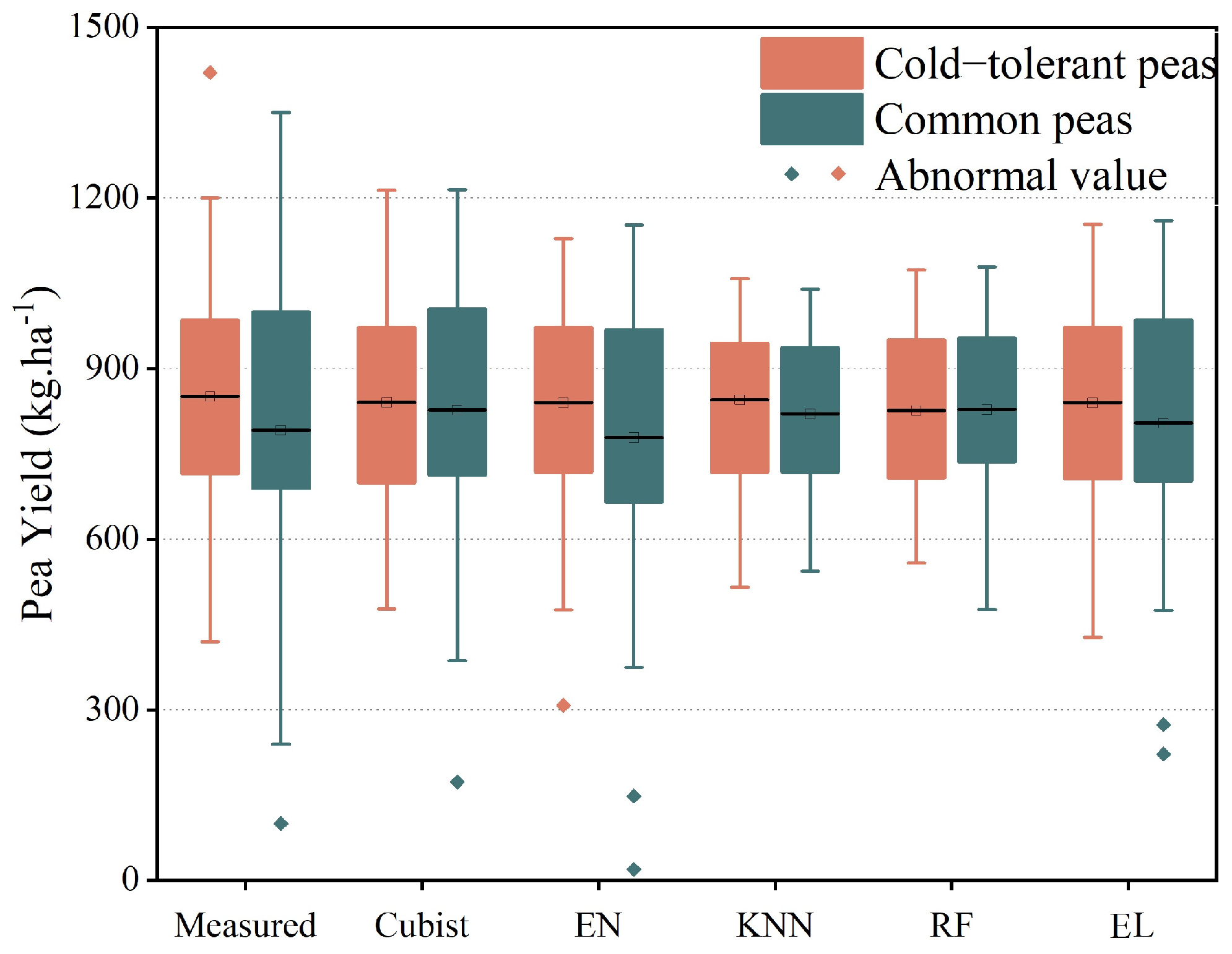
This study tested the applicability of the models by comparing the estimated and measured yields of two different pea types (cold-tolerant and common peas). This section only presents the results obtained under the optimal estimation performance conditions, namely, in the mid filling stage using dual sensors, which has been proven above. As shown in Figure 7, the estimated yield of cold-tolerant peas was slightly higher than that of common peas, which is consistent with the measured values. The estimated yield, therefore, did not significantly change with pea type, thereby reflecting a satisfactory adaptability of the yield estimation models to the two types of peas investigated in this study.

3.5. Estimation Effect Analysis

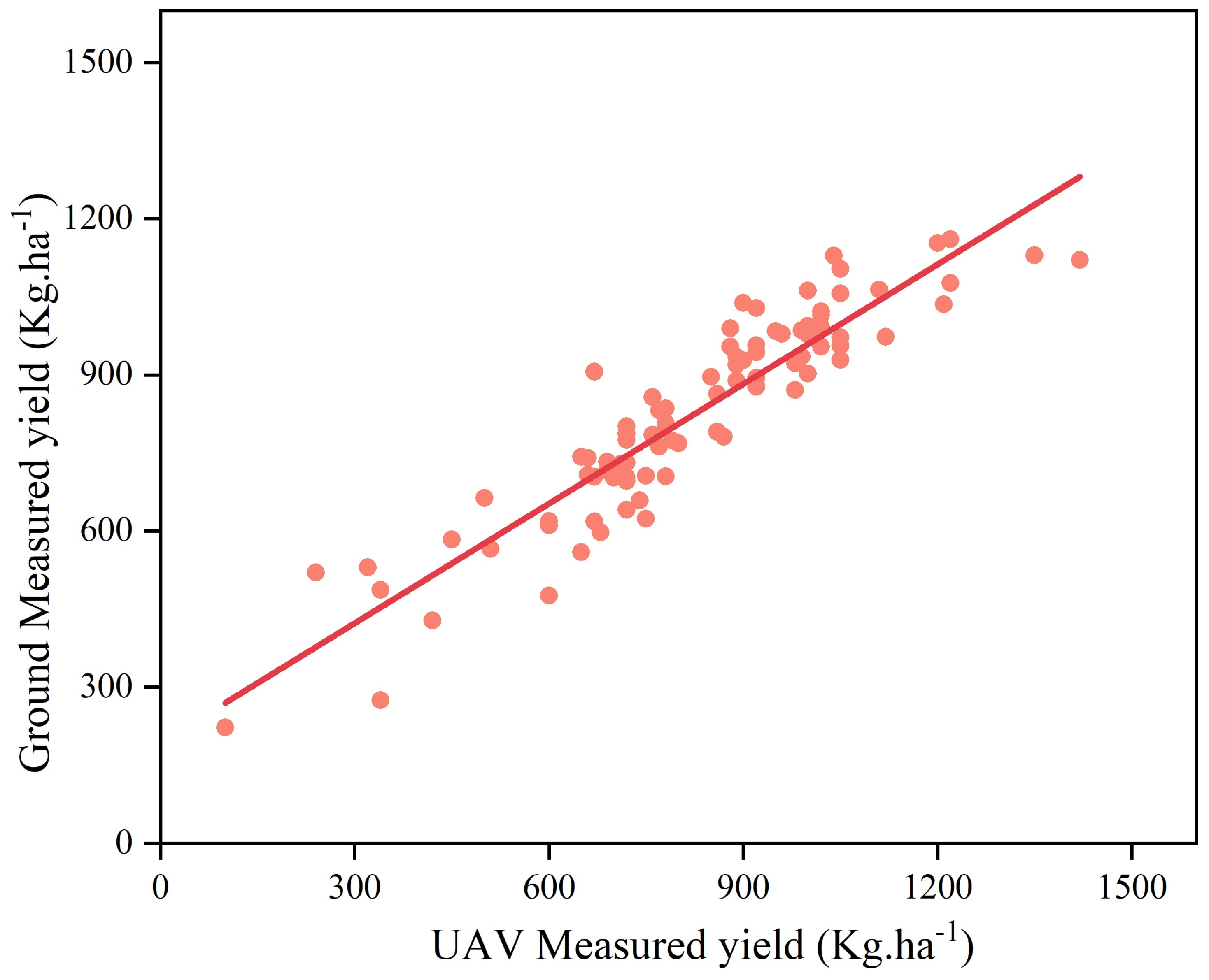
The fusion of RGB and MS data show the best pea yield estimates in the mid filling stage. Hence, the absolute differential values between the estimated and measured values at the mid filling stage were then used to generate a heat map with EL and four base learners (Figure 8). From a visual perspective, smaller color differences represent better estimation accuracy, in which the EL provided superior estimates, followed by the EN and Cubist, the KNN presented the worst estimation accuracy, which is consistent with the results in Section 3.3. In conclusion, the most reliable yield estimation can be obtained using the appropriate algorithm and the fusion of dual-sensor data in the mid filling stage, and the scatter plot between the estimated yield and the ground yield is shown in Figure 9.

4. Discussion

4.1. The Estimation Accuracy between Different Sensors

RGB and MS images based on UAVs have been successfully applied to a majority of crop yield estimations, and their applicability and accuracy also have been confirmed by reports in the literature. However, up to now, the estimation of pea yield based on UAV imagery has not been explored. In this study, RGB and MS sensors were first introduced to estimate pea yield. The estimation accuracy of RGB sensor outperformed that of the MS sensor in the early growth stage. This is likely due to the RGB images has a higher spatial resolution than MS [40]. Another probable reason is that PH and CC were conducive to the improvement of the estimation accuracy [33], which implies that the contribution of structural information is greater than spectral information in early growth stage. However, the estimation accuracy of the MS sensor outperformed the RGB sensor in the mid and late growth stages. This is likely related to the following reasons. Firstly, the MS sensor provides the reflectance of five bands, which makes the spectral information more comprehensive, and the red-edge and near-infrared spectra have been demonstrated to improve the yield estimation accuracy [46]. Secondly, the VIs derived from MS performed better than those derived from RGB [47], and the contributions of the spectral information and vegetation index were greater than that of the structural features at this point.
This study demonstrates that the fusion of both sensors (RGB + MS) obtained the best pea yield estimation results in all five growth stages, with R2 values reaching 0.805. Previous studies have shown that the fusion data achieved higher estimation accuracy than using a single sensor [36], which is consistent with the results obtained here. This may be attributed to the fact that canopy structure information from RGB sensor can overcome the problem of asymptotic saturation inherent in spectral features to a certain extent [48], while the MS spectral information can resolve the problem that RGB spectral information is generally not comprehensive. Because MS and RGB sensors are less costly and a drone can carry two sensors at the same time, the obtained fusion data therefore provide an improved estimation result compared to that obtained using a single sensor, which can provide a new optimized choice for estimating the yields of other legumes in the future.

4.2. Effects of Pea Growth Stage on Estimating Pea Yield

Previous studies have reported multi-source sensors in estimating crop yields, but most have focused on a single growth stage; this study makes up for this deficiency. Some studies have suggested that different growth stages may influence the sensitivity of the vegetation index for yield estimations [49], which is well reflected in this study. Additionally, the reason for the fluctuation at flowering stage could be attributed to the strong correlation between the CC and yield at the branching stage. However, the CC peaks at the flowering stage, leading to a decline in yield estimation performance. Depending on the purpose of the estimation, different growth stages should be selected, in which the mid filling stage is the best choice if the purpose is to estimate the yield for estimating economic value ahead of time. However, if the purpose is to make future seeding plans by estimating yield, the early filling stage will be the best choice because the mid filling stage estimates are obtained too late.

4.3. Performance of Models for Pea Yield Estimation

Machine learning algorithms combined with UAV-based images have been demonstrated to be practical for estimating the yields of certain crops [50]. Each algorithm has its own characteristics, and selecting the appropriate one can greatly impact the yield estimation.
This study found that the Cubist and EN algorithms performed the best. This result is consistent with previous findings to a certain extent [50,51]. The accuracy of the yield estimations obtained using the KNN algorithm failed to obtain satisfactory results. This maybe due to the fact that the KNN is highly dependent on the training data and is more suitable for classification applications [52].
The development of ensemble learning has provided a better choice for estimating yield. The improved performance of ensemble learning may be attributed to its ability to minimize the biases and stochasticity of the underlying base models to a great extent. This finding is consistent with the results that Shu et al. reported, which revealed that the EL model achieved superior estimation accuracy when utilized to estimate maize phenotypic traits [53].

4.4. The Estimation Accuracy between Two Types of Peas

There was no significant difference in the ability of the machine learning algorithms on estimating two types of peas (cold-tolerant and common) in this study. The common peas achieved a higher estimation yield than cold-tolerant peas, which is consistent with the measured pea yield. Previous studies have shown that, although different crop varieties exhibit different phenotypic characteristics, UAV-based high-throughput plant phenotypes were accurate and repeatable for yield estimation [52]. This result, obtained in the present work, is consistent with those previous findings.

4.5. Deficiency and Prospect

Although this study has made some achievements in estimating pea yield, it was limited to a single year and location, and the early growth stages of estimation performance are not satisfactory.
In future research, multi-sensor data fusion and EL will play an increasingly important role, and estimation accuracy can be improved by incorporating more phenotypic traits [35]. While emphasizing the estimation accuracy of the model, the applicability should not be ignored. Multiple years and sites of experiments are an effective way to improve model applicability. Other studies have shown that deep learning methods exhibit a good performance in estimating phenotypic traits [54], which may also be one of the development directions for pea yield estimations in the future. Additionally, weather conditions, the physical and chemical qualities of soil, soil microbe community, and numerous other features are also closely related to yield [35]. These parameters should therefore be reasonably obtained for use as quantitative inputs or estimation models in further research to allow the model to achieve a better estimation performance.

5. Conclusions

This paper applied RGB and MS sensors and their fusion data to estimate pea yield in five growth stages of two pea types and explored the performance of four base algorithms (Cubist, EN, RF, and KNN) and EL. The results are as follows:
(1)
The RGB estimation accuracy outperformed the MS data in the early growth stage, whereas the MS estimation accuracy was higher in the late growth stage. Regardless of growth stage, the fusion data (RGB + MS) obtained higher accuracy than the single-sensor estimation of pea yield.
(2)
The mid filling growth stage achieved the best estimation of pea yield than the other four growth stages, whereas the branching and flowering growth stages were poor.
(3)
The EN and Cubist algorithms performed better than the RF and KNN algorithms in estimating pea yield, and the EL algorithm provided the best performance in estimating pea yield than base learners.
(4)
The applicability of the estimation method was verified by comparing the yield estimation effect of cold-tolerant and common pea types. This study thereby provides technical support and valuable insight for future pea yield estimations.

Supplementary Materials

The following supporting information can be downloaded at: https://www.mdpi.com/article/10.3390/drones8060227/s1, Table S1: Description of VIs from the RGB images; Table S2: Description of VIs from the MS images; Table S3: Pea yield estimation accuracy using the Cubist, EN, KNN, and RF algorithms.

Author Contributions

Z.L. (Zehao Liu): Investigation, Visualization, Writing—original draft. Y.J.: Project administration, Investigation, Writing—original draft. X.Y.: Collecting samples. R.L.: Collecting samples. X.Z.: Resources, Funding acquisition. Z.L. (Zhenxing Liu): Resources, Funding acquisition. T.Y.: Supervision, Funding acquisition, Writing—review and editing. All authors have read and agreed to the published version of the manuscript.

Funding

This work was funded by the Key R&D Program of Hebei Province (No. 22326310D), the fund for State Key Laboratory of Crop Gene Resources and Breeding, the earmarked fund for China Agriculture Research System (CARS-08), National Crop Genebank project from the Ministry of Science and Technology of China (NCGRC-2023-7), and the Agricultural Science and Technology Innovation Program in CAAS.

Data Availability Statement

The datasets used and/or analyzed during the current study are available from the corresponding author on reasonable request.

Conflicts of Interest

The authors declare no competing interests.

References

  1. Sharma, N.K.; Ban, Z.; Classen, H.L.; Yang, H.; Yan, X.; Choct, M.; Wu, S.B. Net energy, energy utilization, and nitrogen and energy balance affected by dietary pea supplementation in broilers. Anim. Nutr. 2021, 7, 506–511. [Google Scholar] [CrossRef] [PubMed]
  2. Zhang, X.; Wan, S.; Hao, J.; Hu, J.; Yang, T.; Zong, X. Large-scale evaluation of pea (Pisum sativum L.) germplasm for cold tolerance in the field during winter in Qingdao. Crop J. 2016, 4, 377–383. [Google Scholar] [CrossRef]
  3. Li, Y.X. Cultivated land and food supply in China. Land Use Policy 2000, 7, 73–88. [Google Scholar]
  4. Bastiaanssen, W.; Ali, S. A new crop yield forecasting model based on satellite measurements applied across the Indus Basin, Pakistan. Agric. Ecosyst. Environ. 2003, 94, 321–340. [Google Scholar] [CrossRef]
  5. Allen, R.; Hanuschak, G.; Craig, M. Limited Use of Remotely Sensed Data for Crop Condition Monitoring and Crop Yield Forecasting in NASS; US Department of Agriculture: Washington, DC, USA, 2002.
  6. Geipel, J.; Link, J.; Claupein, W. Combined Spectral and Spatial Modeling of Corn Yield Based on Aerial Images and Crop Surface Models Acquired with an Unmanned Aircraft System. Remote Sens. 2014, 6, 10335–10355. [Google Scholar] [CrossRef]
  7. Battude, M.; Al Bitar, A.; Morin, D.; Cros, J.; Huc, M.; Sicre, C.M.; Le Dantec, V.; Demarez, V. Estimating maize biomass and yield over large areas using high spatial and temporal resolution Sentinel-2 like remote sensing data. Remote Sens. Environ. 2016, 184, 668–681. [Google Scholar] [CrossRef]
  8. Xie, Y.; Huang, J. Integration of a Crop Growth Model and Deep Learning Methods to Improve Satellite-Based Yield Estimation of Winter Wheat in Henan Province, China. Remote Sens. 2021, 13, 4372. [Google Scholar] [CrossRef]
  9. Yu, D.; Zha, Y.; Shi, L.; Jin, X.; Hu, S.; Yang, Q.; Huang, K.; Zeng, W. Improvement of sugarcane yield estimation by assimilating UAV-derived plant height observations. Eur. J. Agron. 2020, 121, 126159. [Google Scholar] [CrossRef]
  10. Anthony, D.; Elbaum, S.; Lorenz, A.; Detweiler, C. On crop height estimation with UAVs. In Proceedings of the IEEE/RSJ International Conference on Intelligent Robots & Systems, Chicago, IL, USA, 14–18 September 2014. [Google Scholar]
  11. Falco, N.; Wainwright, H.M.; Dafflon, B.; Ulrich, C.; Soom, F.; Peterson, J.E.; Brown, J.B.; Schaettle, K.B.; Williamson, M.; Cothren, J.D.; et al. Influence of soil heterogeneity on soybean plant development and crop yield evaluated using time-series of UAV and ground-based geophysical imagery. Sci. Rep. 2021, 11, 7046. [Google Scholar] [CrossRef] [PubMed]
  12. Radoglou-Grammatikis, P.; Sarigiannidis, P.; Lagkas, T.; Moscholios, I. A compilation of UAV applications for precision agriculture. Comput. Netw. 2020, 172, 107148. [Google Scholar] [CrossRef]
  13. Fei, S.; Hassan, M.A.; He, Z.; Chen, Z.; Shu, M.; Wang, J.; Li, C.; Xiao, Y. Assessment of Ensemble Learning to Predict Wheat Grain Yield Based on UAV-Multispectral Reflectance. Remote Sens. 2021, 13, 2338. [Google Scholar] [CrossRef]
  14. Peng, X.; Han, W.; Ao, J.; Wang, Y. Assimilation of LAI Derived from UAV Multispectral Data into the SAFY Model to Estimate Maize Yield. Remote Sens. 2021, 13, 1094. [Google Scholar] [CrossRef]
  15. Song, Y.; Wang, J.; Shang, J.; Liao, C. Using UAV-Based SOPC Derived LAI and SAFY Model for Biomass and Yield Estimation of Winter Wheat. Remote Sens. 2020, 12, 2378. [Google Scholar] [CrossRef]
  16. Vega, F.A.; Ramírez, F.C.; Saiz, M.P.; Rosúa, F.O. Multi-temporal imaging using an unmanned aerial vehicle for monitoring a sunflower crop. Biosyst. Eng. 2015, 132, 19–27. [Google Scholar] [CrossRef]
  17. Li, C.; Ma, C.; Cui, Y.; Lu, G.; Wei, F. UAV Hyperspectral Remote Sensing Estimation of Soybean Yield Based on Physiological and Ecological Parameter and Meteorological Factor in China. J. Indian Soc. Remote Sens. 2020, 49, 873–886. [Google Scholar] [CrossRef]
  18. Varela, S.; Pederson, T.; Bernacchi, C.J.; Leakey, A.D.B. Understanding Growth Dynamics and Yield Prediction of Sorghum Using High Temporal Resolution UAV Imagery Time Series and Machine Learning. Remote Sens. 2021, 13, 1763. [Google Scholar] [CrossRef]
  19. Kefauver, S.C.; Vicente, R.; Vergara-Diaz, O.; Fernandez-Gallego, J.A.; Kerfal, S.; Lopez, A.; Melichar, J.P.E.; Serret Molins, M.D.; Araus, J.L. Comparative UAV and Field Phenotyping to Assess Yield and Nitrogen Use Efficiency in Hybrid and Conventional Barley. Front. Plant Sci. 2017, 8, 1733. [Google Scholar] [CrossRef]
  20. Feng, A.; Zhou, J.; Vories, E.D.; Sudduth, K.A.; Zhang, M. Yield estimation in cotton using UAV-based multi-sensor imagery. Biosyst. Eng. 2020, 193, 101–114. [Google Scholar] [CrossRef]
  21. Som-ard, J.; Hossain, M.D.; Ninsawat, S.; Veerachitt, V. Pre-harvest Sugarcane Yield Estimation Using UAV-Based RGB Images and Ground Observation. Sugar Tech 2018, 20, 645–657. [Google Scholar] [CrossRef]
  22. Stroppiana, D.; Migliazzi, M.; Chiarabini, V.; Crema, A.; Musanti, M.; Franchino, C.; Villa, P. Rice yield estimation using multispectral data from UAV: A preliminary experiment in northern Italy. In Proceedings of the 2015 IEEE International Geoscience and Remote Sensing Symposium, Milan, Italy, 26–31 July 2015; pp. 4664–4667. [Google Scholar]
  23. Luo, B.; Yang, C.; Chanussot, J.; Zhang, L. Crop Yield Estimation Based on Unsupervised Linear Unmixing of Multidate Hyperspectral Imagery. IEEE Trans. Geosci. Remote Sens. 2013, 51, 162–173. [Google Scholar] [CrossRef]
  24. Gené-Mola, J.; Gregorio, E.; Cheein, F.A.; Guevara, J.; Llorens, J.; Sanz-Cortiella, R.; Escolà, A.; Rosell-Polo, J.R. Fruit detection, yield prediction and canopy geometric characterization using LiDAR with forced air flow. Comput. Electron. Agric. 2020, 168, 105121. [Google Scholar] [CrossRef]
  25. Zhang, M.; Zhou, J.; Sudduth, K.A.; Kitchen, N.R. Estimation of maize yield and effects of variable-rate nitrogen application using UAV-based RGB imagery. Biosyst. Eng. 2020, 189, 24–35. [Google Scholar] [CrossRef]
  26. Huang, Y.; Sui, R.; Thomson, S.J.; Fisher, D.K. Estimation of cotton yield with varied irrigation and nitrogen treatments using aerial multispectral imagery. Int. J. Agric. Biol. Eng. 2013, 6, 37–41. [Google Scholar]
  27. García-Martínez, H.; Flores-Magdaleno, H.; Ascencio-Hernández, R.; Khalil-Gardezi, A.; Tijerina-Chávez, L.; Mancilla-Villa, O.R.; Vázquez-Peña, M.A. Corn Grain Yield Estimation from Vegetation Indices, Canopy Cover, Plant Density, and a Neural Network Using Multispectral and RGB Images Acquired with Unmanned Aerial Vehicles. Agriculture 2020, 10, 277. [Google Scholar] [CrossRef]
  28. Li, Q.; Jin, S.; Zang, J.; Wang, X.; Sun, Z.; Li, Z.; Xu, S.; Ma, Q.; Su, Y.; Guo, Q.; et al. Deciphering the contributions of spectral and structural data to wheat yield estimation from proximal sensing. Crop J. 2022, 10, 1334–1345. [Google Scholar] [CrossRef]
  29. Ashapure, A.; Jung, J.; Chang, A.; Oh, S.; Yeom, J.; Maeda, M.; Maeda, A.; Dube, N.; Landivar, J.; Hague, S.; et al. Developing a machine learning based cotton yield estimation framework using multi-temporal UAS data. ISPRS J. Photogramm. Remote Sens. 2020, 169, 180–194. [Google Scholar] [CrossRef]
  30. Guo, Y.; Wang, H.; Wu, Z.; Wang, S.; Sun, H.; Senthilnath, J.; Wang, J.; Bryant, C.R.; Fu, Y. Modified Red Blue Vegetation Index for Chlorophyll Estimation and Yield Prediction of Maize from Visible Images Captured by UAV. Sensors 2020, 20, 5055. [Google Scholar] [CrossRef] [PubMed]
  31. Ji, Y.; Liu, R.; Xiao, Y.; Cui, Y.; Chen, Z.; Zong, X.; Yang, T. Faba bean above-ground biomass and bean yield estimation based on consumer-grade unmanned aerial vehicle RGB images and ensemble learning. Precis. Agric. 2023, 24, 1439–1460. [Google Scholar] [CrossRef]
  32. Thenkabail, P.S.; Smith, R.B.; Pauw, E.D. Hyperspectral Vegetation Indices and Their Relationships with Agricultural Crop Characteristics. Remote Sens. Environ. 2000, 71, 158–182. [Google Scholar] [CrossRef]
  33. Ji, Y.; Chen, Z.; Cheng, Q.; Liu, R.; Li, M.; Yan, X.; Li, G.; Wang, D.; Fu, L.; Ma, Y.; et al. Estimation of plant height and yield based on UAV imagery in faba bean (Vicia faba L.). Plant Methods 2022, 18, 26. [Google Scholar] [CrossRef] [PubMed]
  34. Shu, M.; Shen, M.; Dong, Q.; Yang, X.; Li, B.; Ma, Y. Estimating the maize above-ground biomass by constructing the tridimensional concept model based on UAV-based digital and multi-spectral images. Field Crops Res. 2022, 282, 108491. [Google Scholar] [CrossRef]
  35. Liu, S.; Jin, X.; Nie, C.; Wang, S.; Yu, X.; Cheng, M.; Shao, M.; Wang, Z.; Tuohuti, N.; Bai, Y.; et al. Estimating leaf area index using unmanned aerial vehicle data: Shallow vs. deep machine learning algorithms. Plant Physiol. 2021, 187, 1551–1576. [Google Scholar] [CrossRef] [PubMed]
  36. Maimaitijiang, M.; Sagan, V.; Sidike, P.; Hartling, S.; Esposito, F.; Fritschi, F.B. Soybean yield prediction from UAV using multimodal data fusion and deep learning. Remote Sens. Environ. 2020, 237, 111599. [Google Scholar] [CrossRef]
  37. Nichol, J.E.; Sarker, M.L.R. Improved Biomass Estimation Using the Texture Parameters of Two High-Resolution Optical Sensors. IEEE Trans. Geosci. Remote Sens. 2011, 49, 930–948. [Google Scholar] [CrossRef]
  38. Quinlan, J.R. Learning with continuous classes. In Proceedings of the 5th Australian Joint Conference on Artificial Intelligence, Hobart, TAS, Australia, 16–18 November 1992. [Google Scholar]
  39. Houborg, R.; McCabe, M.F. A hybrid training approach for leaf area index estimation via Cubist and random forests machine-learning. ISPRS J. Photogramm. Remote Sens. 2018, 135, 173–188. [Google Scholar] [CrossRef]
  40. Fei, S.; Hassan, M.A.; Xiao, Y.; Su, X.; Chen, Z.; Cheng, Q.; Duan, F.; Chen, R.; Ma, Y. UAV-based multi-sensor data fusion and machine learning algorithm for yield prediction in wheat. Precis. Agric. 2022, 24, 187–212. [Google Scholar] [CrossRef]
  41. Cong, H.; Xjwa, B.; Zyl, C. Generating adversarial examples with elastic-net regularized boundary equilibrium generative adversarial network—ScienceDirect. Pattern Recognit. Lett. 2020, 140, 281–287. [Google Scholar]
  42. Gang, Z.; Peng, S.K.; Rong, H.; Yang, L.I.; Wang, N. A General Introduction to Estimation and Retrieval of Forest Volume with Remote Sensing Based on KNN. Remote Sens. Technol. Appl. 2010, 34, 2627–2638. [Google Scholar]
  43. Breiman, L. Machine Learning. Mach. Learn. 2001, 45, 5–32. [Google Scholar] [CrossRef]
  44. Lujan-Moreno, G.A.; Howard, P.R.; Rojas, O.G.; Montgomery, D.C. Design of experiments and response surface methodology to tune machine learning hyperparameters, with a random forest case-study. Expert Syst. Appl. 2018, 109, 195–205. [Google Scholar] [CrossRef]
  45. Wolpert, D.H. Stacked generalization. Neural Netw. 1992, 5, 241–259. [Google Scholar] [CrossRef]
  46. Hassani, K.; Gholizadeh, H.; Taghvaeian, S.; Natalie, V.; Carpenter, J.; Jacob, J. Application of UAS-Based Remote Sensing in Estimating Winter Wheat Phenotypic Traits and Yield During the Growing Season. PFG—J. Photogramm. Remote Sens. Geoinf. Sci. 2023, 91, 77–90. [Google Scholar] [CrossRef]
  47. Guo, Y.; Zhang, X.; Chen, S.; Wang, H.; Jayavelu, S.; Cammarano, D.; Fu, Y. Integrated UAV-Based Multi-Source Data for Predicting Maize Grain Yield Using Machine Learning Approaches. Remote Sens. 2022, 14, 6290. [Google Scholar] [CrossRef]
  48. Chang, A.; Jung, J.; Yeom, J.; Maeda, M.M.; Landivar, J.A.; Enciso, J.M.; Avila, C.A.; Anciso, J.R. Unmanned Aircraft System- (UAS-) Based High-Throughput Phenotyping (HTP) for Tomato Yield Estimation. J. Sens. 2021, 2021, 8875606. [Google Scholar] [CrossRef]
  49. Liu, S.; Hu, Z.; Han, J.; Li, Y.; Zhou, T. Predicting grain yield and protein content of winter wheat at different growth stages by hyperspectral data integrated with growth monitor index. Comput. Electron. Agric. 2022, 200, 107235. [Google Scholar] [CrossRef]
  50. Alabi, T.R.; Abebe, A.T.; Chigeza, G.; Fowobaje, K.R. Estimation of soybean grain yield from multispectral high-resolution UAV data with machine learning models in West Africa. Remote Sens. Appl. Soc. Environ. 2022, 27, 100782. [Google Scholar] [CrossRef]
  51. Mbebi, A.J.; Breitler, J.C.; Bordeaux, M.; Sulpice, R.; McHale, M.; Tong, H.; Toniutti, L.; Castillo, J.A.; Bertrand, B.; Nikoloski, Z. A comparative analysis of genomic and phenomic predictions of growth-related traits in 3-way coffee hybrids. G3 2022, 12, jkac170. [Google Scholar] [CrossRef] [PubMed]
  52. Cheng, M.; Jiao, X.; Liu, Y.; Shao, M.; Yu, X.; Bai, Y.; Wang, Z.; Wang, S.; Tuohuti, N.; Liu, S.; et al. Estimation of soil moisture content under high maize canopy coverage from UAV multimodal data and machine learning. Agric. Water Manag. 2022, 264, 107530. [Google Scholar] [CrossRef]
  53. Shu, M.; Fei, S.; Zhang, B.; Yang, X.; Guo, Y.; Li, B.; Ma, Y. Application of UAV Multisensor Data and Ensemble Approach for High-Throughput Estimation of Maize Phenotyping Traits. Plant Phenomics 2022, 2022, 9802585. [Google Scholar] [CrossRef] [PubMed]
  54. Sagan, V.; Maimaitijiang, M.; Bhadra, S.; Maimaitiyiming, M.; Brown, D.R.; Sidike, P.; Fritschi, F.B. Field-scale crop yield prediction using multi-temporal WorldView-3 and PlanetScope satellite data and deep learning. ISPRS J. Photogramm. Remote Sens. 2021, 174, 265–281. [Google Scholar] [CrossRef]
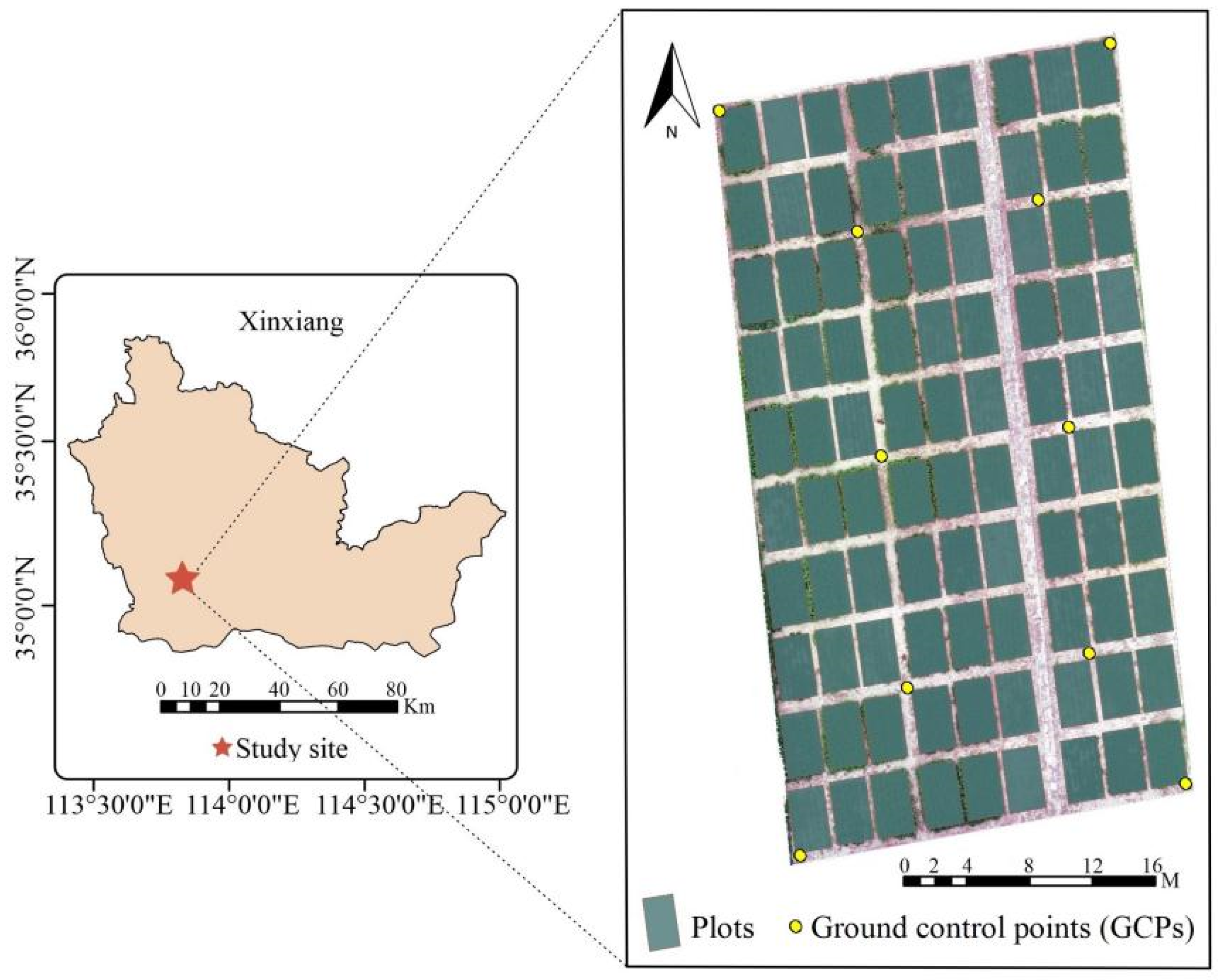
Figure 1. Location and layout of the study site.
Drones 08 00227 g001
Figure 2. UAV observation platform and two sensors: (a) MS sensor; (b) RGB sensor.
Drones 08 00227 g002
Figure 3. A workflow of ensemble learning; EN: elastic net; KNN: K nearest neighbor; RF: random forest; MLR: multiple linear regression.
Drones 08 00227 g003
Figure 4. Comparison of estimation accuracy using different sensors. MS: multi−spectral; RGB + MS: fusion data of RGB and MS; BS: branching stage; FS: flowering stage; PS: podding stage; EFS: early filling stage; MFS: mid filling stage.
Drones 08 00227 g004
Figure 5. Pea yield estimation accuracy in the five growth stages. MS: multi−spectral; RGB + MS: fusion data of RGB and MS; BS: branching stage; FS: flowering stage; PS: podding stage; EFS: early filling stage; MFS: mid filling stage; EN: elastic net; KNN: K nearest neighbor; RF: random forest.
Drones 08 00227 g005
Figure 6. Variation in estimation accuracy (R2) in the different growth stages using the different algorithms. (a): RGB; (b): MS; (c): fusion data of RGB and MS; BS: branching stage; FS: flowering stage; PS: podding stage; EFS: early filling stage; MFS: mid filling stage; EN: elastic net; KNN: K nearest neighbor; RF: random forest.
Drones 08 00227 g006
Figure 7. Comparison of pea yield between ground measurements and UAV estimates. EN: elastic net; KNN: K nearest neighbor; RF: random forest; EL: ensemble learning.
Drones 08 00227 g007
Figure 8. Pictorial diagram of the estimation errors, indicating the absolute differential values between the estimated and measured values. Units = kg·ha−1; EN: elastic net; KNN: K nearest neighbor; RF: random forest; EL: ensemble learning.
Drones 08 00227 g008
Figure 9. Scatter plot of ground-measured and best−estimated yield.
Drones 08 00227 g009
Table 1. Pea growth stages and data collection.
TimeGrowth StagesGround/UAV Data Collection Time
20 September 2019Sowing/
21 September 2019–14 December 2019Seedling stage/
15 December 2019–25 March 2020Branching stage7 March 2020
25 March 2020–10 April 2020Flowering stage3 April 2020
10 April 2020–20 April 2020Podding stage14 April 2020
20 April 2020–28 April 2020Early filling stage14 April 2020
28 April 2020–26 May 2020Mid filling stage14 April 2020
27 May 2020Harvest/
Table 2. Parameters and detailed information of the sensors.
CameraSensorSize(mm)BandImage Resolution
Zenmuse X7 RGB151 × 108 × 132 R G B2400 × 1080
Red-Edge MXMulti-spectral87 × 59 × 45.4Blue 1280 × 960
   Green
Red
1280 × 960
1280 × 960
   Red-edge1280 × 960
   Near infrared1280 × 960
Table 3. Pea yield estimation accuracy using the EL, Cubist, EN, KNN, and RF algorithms based on the dual sensor (RGB + MS).
  CubistENKNNRFEL
BSR20.350.490.200.330.52
 RMSE189.06171.66220.50195.06169.44
 NRMSE22.89%20.79%26.71%23.63%21.80%
FSR20.480.610.240.410.62
 RMSE172.72148.42218.73180.80146.90
 NRMSE20.92%17.97%26.91%21.89%17.69%
PSR20.540.560.400.540.65
 RMSE159.79158.99200.50160.69145.04
 NRMSE19.35%19.26%24.71%19.46%17.91%
EFSR20.590.670.440.630.69
 RMSE149.10136.70186.14149.45127.99
 NRMSE18.05%16.5%22.54%18.10%15.19%
MFSR20.810.800.580.770.85
 RMSE103.00111.05168.79125.94101.16
 NRMSE12.48%13.45%20.44%15.25%12.86%
Note: BS: branching stage; FS: flowering stage; PS: podding stage; EFS: early filling stage; MFS: mid filling stage; EN: elastic net; KNN: K nearest neighbor; RF: random forest; EL: ensemble learning. The bolded terms indicate the best R2, RMSE, and NRMSE values.
Disclaimer/Publisher’s Note: The statements, opinions and data contained in all publications are solely those of the individual author(s) and contributor(s) and not of MDPI and/or the editor(s). MDPI and/or the editor(s) disclaim responsibility for any injury to people or property resulting from any ideas, methods, instructions or products referred to in the content.