UAV Swarm Search Path Planning Method Based on Probability of Containment

Abstract

To improve the search efficiency of the unmanned aerial vehicle (UAV) swarm in disaster areas, the target distribution probability graph in the prior information is introduced, and a drone cluster search trajectory planning method based on probability of containment (POC) is proposed. Firstly, based on the concept of probability of containment in search theory, a task area division method for polygonal and circular areas is constructed, and the corresponding search trajectory is constructed. Then, the influence of factors, including probability of containment, probability of detection, and probability of success on search efficiency, is sorted out, and the objective function of search trajectory optimization is constructed. Subsequently, an adaptive mutation operator is used to improve the differential evolution algorithm, thus constructing a trajectory optimization process based on the improved adaptive differential evolution algorithm. Through simulation verification, the proposed method can achieve a full coverage search of the task area and a rapid search within a limited time, and can prioritize the coverage of areas with a high target existence probability as much as possible to achieve a higher cumulative success probability. Moreover, the time efficiency and accuracy of the solution are high.

1. Introduction

Drones have gradually become an indispensable force in disaster relief. Due to their flexibility and convenience, drones have incomparable advantages over other data collection platforms in terms of data transmission and express delivery [1,2,3]. However, communication interruptions, landslides, and road collapses after earthquakes seriously hinder effective rescue. Therefore, how to use drone clusters to quickly grasp the situation in disaster areas after earthquakes plays a crucial role in formulating rescue plans.

1.1. Related Work

To this end, scholars have conducted in-depth explorations and achieved fruitful results, mainly including environmental modeling, trajectory planning methods based on classical theories, and trajectory planning methods based on intelligent algorithms.

Environmental modeling mainly involves building geographical models [4,5,6,7] and quantifying threats [8,9,10,11,12]. In the literature [4], an elevation map was used to simulate the actual flight environment of UAVs and construct a trajectory optimization method. In the literature [5,6], digital simulation was used to construct the environment from different perspectives to meet the corresponding requirements. The literature [7] further constructed a map from 3D to 2D maps to reduce the complexity of the map. Threats usually include radar and missile threats. To study the impacts of these military equipment and UAV trajectory planning, the literature [8] constructed a threat model for radar and missiles. Based on this, the literature [9] further extended it to the 3D space. The literature [10] further considered the temporal variation of threats during the motion of UAVs to optimize trajectories based on the analysis of previous research work. On this basis, the literature [11] constructed a Bayesian network to evaluate threats. The literature [12] further established a dynamic Bayesian network to study the threats posed by the environment on UAVs when parameters change.

Classic trajectory planning theory mainly includes the artificial potential field method [13,14], A* algorithm [15,16,17], Dijkstra algorithm [18,19], etc. The literature [20] improved the artificial potential field method algorithm and solved it using genetic algorithms. The literature [21] further combined the artificial potential field method with reinforcement learning on its basis, and avoided local optima by setting up black holes. The literature [22] achieved the goal of synchronously arriving at the task area within a specified time by regulating the trajectory intersection points of each unmanned aerial vehicle (UAV) in the cluster. The literature [23], based on the Dubins path planning algorithm, avoided collisions between UAVs by adjusting the trajectory length of UAVs, and achieved a collaborative formation of UAVs. The literature [24], based on graph theory, converted the heading to connectivity constraints in graph theory, and optimized it to achieve spatial collaboration of cluster trajectories. The literature [25,26], based on the idea of dynamic programming, adjusted the angle between each UAV and the target point in the UAV cluster at all times, and achieved the goal of distributing UAVs near the target at different angles at the same time through real-time optimization decisions.

There are mainly two types of intelligent algorithm-based trajectory planning methods. One is to study biological characteristics and further construct new intelligent optimization algorithms to apply them to solving trajectory planning problems, such as the wolf swarm algorithm [27,28], firefly swarm algorithm [29,30], and fruit fly swarm optimization algorithm [31,32]. The other is to improve the performance of algorithms by optimizing parameters, improving the algorithm architecture, or integrating with other algorithms. The literature [33] used the principle of pheromone diffusion to improve the ant colony algorithm, thereby enhancing the ability of UAV trajectory planning in complex environments. The literature [34] used chaos theory to adjust the population distribution of the bee colony algorithm, improving the diversity of the population and thereby performing trajectory planning better. The literature [35] improved the particle swarm algorithm by phase encoding and introducing quantum behavior, thereby enhancing the robustness of the planning algorithm. The literature [36] combined a particle swarm algorithm with a genetic algorithm to achieve trajectory planning in a three-dimensional environment. The literature [37] combined fuzzy logic with an improved artificial bee colony algorithm to optimize the most efficient and safest path.

A summary and comparison of the two types of algorithms are shown in

Table 1. Comparison between classic methods and intelligent methods.

	Classic Method	Intelligent Method
Theoretical model	Yes	No
Type of problem to be solved	Convex optimization	No requirement
Number of problems to be solved	Less	More
General applicability	Poor	Good
Algorithm efficiency	High	Low

.

Table 1 compares the two types of algorithms from five aspects. In terms of theoretical models, classical algorithms have solid theoretical analysis and proof processes, ensuring the feasibility and effectiveness of the algorithm from a mathematical perspective. Most intelligent algorithms are derived from biological inspiration, and there is almost no complete proof process.

In terms of problem types, classical methods solve convex optimization problems. Meanwhile, there are no clear requirements for intelligent algorithms, so they can solve a wider range of problems.

Classic algorithms are built for specific problems, so they can only solve a certain type of problem and are highly targeted. Intelligent algorithms, on the other hand, are generally built by scholars themselves and can be designed and improved based on the problem. They can solve a wide range of problems.

In terms of generality, classical algorithm models are generally used directly to solve problems, but they do not have the ability to adjust the model based on the problem. However, based on the intelligent optimization solving process, both the model and intelligent optimization method can be adjusted and improved according to the needs, which have good generality.

In terms of algorithm efficiency, the solution process of classical methods is generally based on optimization theory, which can quickly obtain optimal results. However, intelligent optimization algorithms require continuous optimization and iteration through a large number of populations, which makes the algorithm slower.

Namely, classical algorithms are more suitable for solving problems for which they have already built models, and they have fast algorithm speeds and solid theoretical support. Intelligent algorithms can build models based on the problem to solve more complex, more closely problems related to actual needs.

1.2. Research Gap and Problem Statement

The current research has a good guiding role in enhancing the flight path planning and search capabilities of drones, and lays a research framework that can be used for the study of such problems. However, there are still practical problems and constraints that need to be addressed.

Drone clusters are widely used in search and rescue missions due to their high cost-effectiveness. With the support of satellites, intelligence, and other platforms of reconnaissance methods, prior information of some task areas is usually known and converted into a target probability distribution map of the area. Making full use of this prior information to carry out search tasks plays an important role in improving the timeliness and success rate of search tasks. However, the current literature mainly studies trajectory planning from both static and dynamic perspectives. Most static trajectory planning methods do not consider the target probability distribution map, divide the search area according to certain criteria, and plan the search trajectory within each sub-area. Dynamic trajectory planning methods use the target probability distribution map to guide the drone cluster to carry out search tasks in real time. However, this method puts stringent requirements on cluster communication and real-time decision-making, which is difficult to achieve in complex environments.

1.3. Proposed Solution and Contributions

To this end, this paper constructs a method for UAV cluster search trajectory planning based on prior information to improve the search efficiency of the cluster. Based on the static trajectory planning method, this paper makes full use of the target probability distribution diagram and introduces the concept of probability of containment (POC) in search theory to optimize the search efficiency of the UAV cluster. A method for UAV cluster search trajectory planning with probability of containment optimization is proposed.

Compared with existing methods, the main contributions of this article are as follows:

• A probability-based track optimization model is constructed. At present, academic papers mainly consider the search process as a deterministic event. Specifically, after a UAV searches a certain area, it will only obtain binary results, namely, there is a target or there is no target. Obviously, due to limitations of UAV performance or image processing, there may be a possibility of searching but not detecting the target. Therefore, the search result should be a probability. Therefore, this article introduces the probability of detection (POD) to describe the probability of discovering the target so that the method is more closely related to reality.
• The objective function can be adjusted according to the task requirements. A search mainly includes two typical requirements, namely, achieving global search with minimal resource consumption and searching as many areas as possible within a limited time. The main achievements at this stage are generally focused on one specific problem. However, the objective function designed in this article can achieve these two goals by changing the corresponding coefficients.
• A more flexible search strategy is constructed. For search tasks, the parallel line search method is highly efficient and easy to implement. However, such methods are applicable to rectangular regions. To improve search performance, this article improves it and designs three other new search methods. The objects searched in this article can be extended to irregular polygonal regions and even circular regions.
• Intelligent optimization algorithms are improved in combination with the problem to be optimized. Some articles that use intelligent optimization to solve trajectory problems have a weak connection between the method and the problem. Namely, intelligent optimization methods are just a tool, and they are not improved in combination with the problem to be optimized, resulting in a low degree of adaptation between the two. The method in this article aims at the problem to be optimized, designs an adaptive mutation algorithm, and constructs a coding method for drones to improve search efficiency.

First, a new search area allocation method and corresponding trajectory planning model are constructed in Section 2. Then, factors affecting search efficiency are analyzed and a search objective function is established in Section 3. In order to optimize the objective function, an adaptive differential evolution algorithm and corresponding optimization process are constructed in Section 4 and Section 5. Experiments are conducted to verify and draw conclusions in Section 6 and Section 7.

2. New Region Division Strategy and Corresponding Route Optimization Method

The target probability distribution map is the prerequisite for search trajectory planning, providing prior information support for search task area planning and trajectory planning. Based on obtaining the target probability distribution map, the search task planning of the unmanned aerial vehicle mainly consists of two parts: search area division and search trajectory planning.

2.1. Search Area Allocation Method Based on the Average Probability of Containment

Due to objective factors such as drone search resources, search hardware capabilities, and time windows, there are often not enough search resources to fully cover all areas where the target may exist. The key issues at this point are what kind of drone to use, where to search, and what search method to use to maximize the search success rate. Search area allocation should consider the performance of the drone and the task requirements, and prioritize searching areas with a high probability of target presence in the target probability distribution map as much as possible.

This section mainly introduces polygon areas and search base circle areas, and gives the corresponding optimal allocation criteria for search areas.

The search reference is the reference basis for determining the search area, which is calculated based on the target’s approximate location, motion characteristics, and environmental information. It mainly consists of the following three types: reference point, reference line, and reference plane. The reference point is the case where the target’s approximate location is known. The probability distribution is calculated based on the target’s motion characteristics, and the point with the highest probability of target existence is determined as the reference point. The reference line is the case where there are two or more possible locations for the target’s approximate location. The reference line is determined based on the connection between multiple approximate locations. In cases where one or more target approximate location points cannot be determined, the reference plane is usually used, which refers to a certain area where the target existence probability is higher than a threshold value.

In order to determine more universal and accurate search area types, the types of reference points, reference lines, and reference planes were summarized, generalized, and improved, and two types of area types, polygon areas and search base circle areas, were proposed. These two types of area types can cover the three reference areas mentioned above, and facilitate a more accurate determination of the search area.

The information of the polygon region is represented by the coordinates of the region’s vertices. Assuming that there are n vertices in the selected search polygon region, their coordinates are p₁, p₂, …, p_n. Assuming that m polygon regions are planned in the search region, the ith polygon is denoted by the following symbol:

$${\mathsf{\Omega }}_p^{\left(i\right)}=\left(p_1^{\left(i\right)},p_2^{\left(i\right)},\dots ,p_{n_i}^{\left(i\right)}\right),i=1,2,\dots ,m$$

(1)

The search base circle domain is a combination of the reference point and the reference plane. It is a circular area determined by taking the point with the highest probability of target existence as the center c and determining the search radius r based on the coverage of the reference plane. Assuming that k search base circle domains are planned in the search area, the ith circle domain is denoted by the following symbol:

$${\mathsf{\Omega }}_c^{\left(i\right)}=\left(c^{\left(i\right)},r^{\left(i\right)}\right),i=1,2,\dots ,k$$

(2)

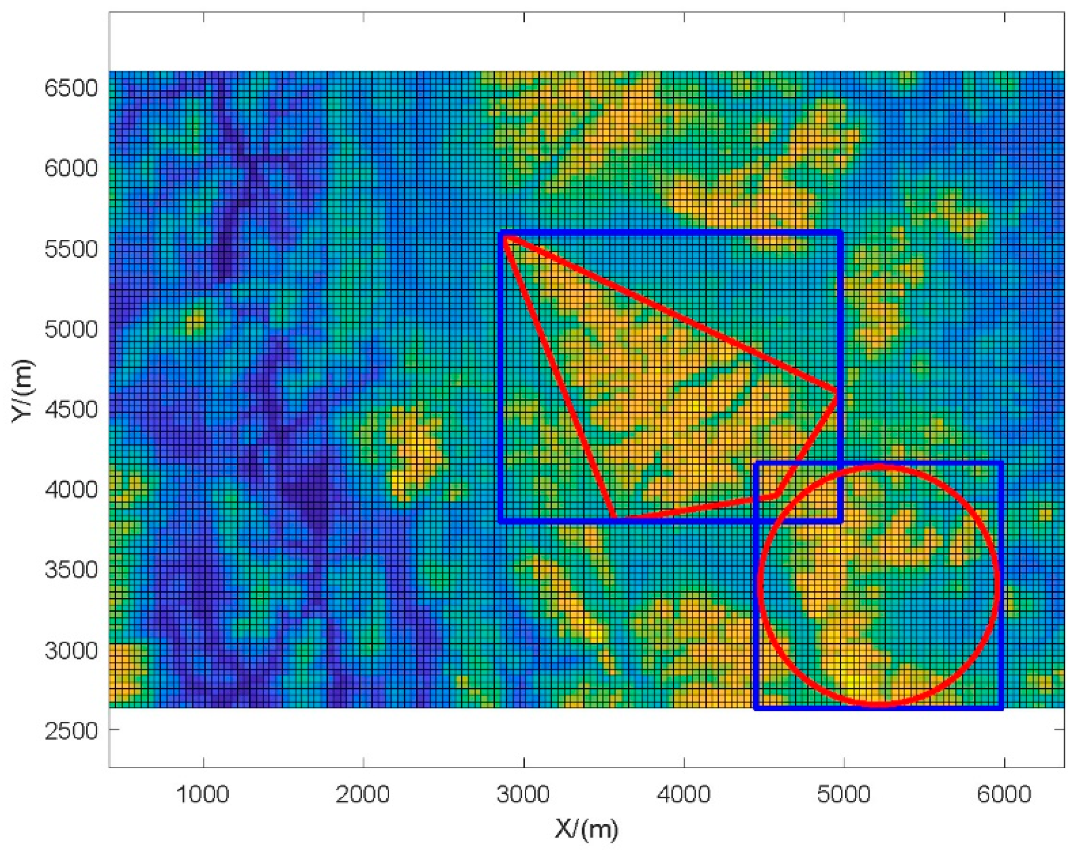
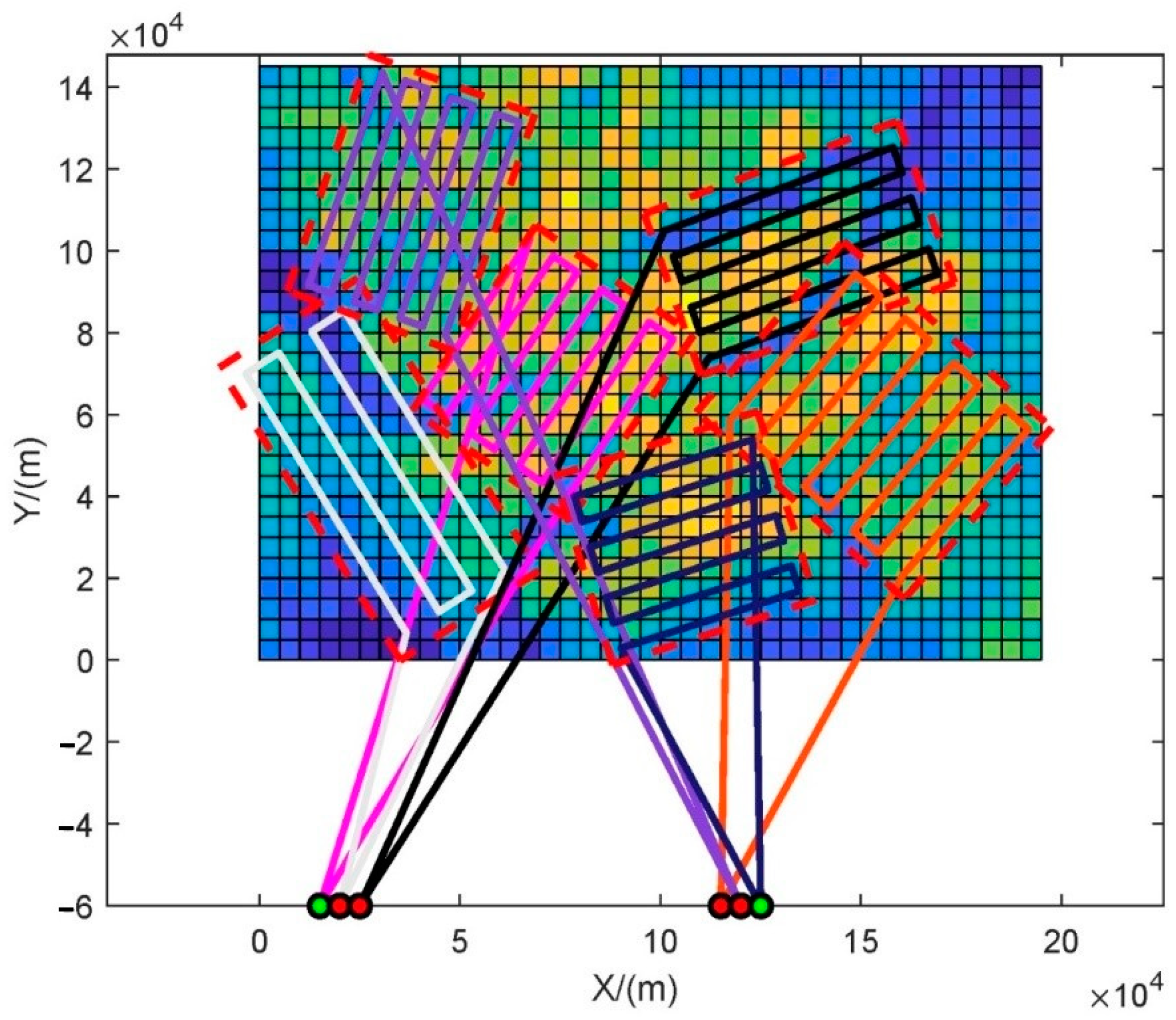
To verify the advantages of polygonal areas and search base circle areas over classic area types, a simple example is given through simulation. The first method uses search rectangles for area planning, while the second method uses polygonal areas and search base circle areas. The planning results are shown in Figure 1.

As can be seen in Figure 1, the red area represents the polygon area and search base circle area, which can more accurately select the area with a high probability of target existence, facilitating the avoidance of overlap between multiple areas. In contrast, the search rectangle represented by the blue area inevitably includes areas with a low probability of target existence in the search range, which results in the additional consumption of search resources and reduces search efficiency. Figure 1 demonstrates the advantages of the two proposed types of search areas in accurately selecting the search area, laying the foundation for subsequent search area optimization and search trajectory planning.

Search area optimization refers to the process of minimizing the search resources and maximizing the target coverage probability within the planned search area under the constraints of drone capabilities and time windows.

The amount of search resources used can be represented by the area of the search region. The larger the search region, the longer the search time and the more search resources required.

The probability of coverage targets can be represented by the sum of the probabilities of inclusion within the search area. The definition of probability of containment (POC) is the probability that a search target is within a certain area, partition, or grid cell.

Combining the two indicators above, we set the optimization criterion for the search area as the average POC, which is the target POC per unit area, as follows:

$$f\left(\mathsf{\Omega }\right)=\frac{{\displaystyle \sum _{i\in \mathsf{\Omega }}{\mathrm{POC}}_i}}{S\left(\mathsf{\Omega }\right)}$$

(3)

where the numerator represents the sum of the probability of target inclusion in the search area, and the denominator represents the area of the search area.

If multiple search areas are planned at the same time, there may be overlap between the areas. Therefore, considering the overlap of areas and assuming that n search areas are planned, the average POC of these n search areas is:

$$f\left(\mathsf{\Omega }\right)=\frac{{\displaystyle \sum _{i\in \mathsf{\Omega }}{\mathrm{POC}}_i}}{S\left({\mathsf{\Omega }}_1\right)+S\left({\mathsf{\Omega }}_1\right)+\cdots S\left({\mathsf{\Omega }}_n\right)}$$

(4)

As can be seen in the Formula (4), the area of the overlapping part of each search region is superimposed, but the target inclusion probability is taken only once. This optimization criterion provides a quantitative standard for planning search regions, enabling a rapid comparison of the advantages and disadvantages of multiple region planning results.

As can be seen in Figure 1, the division and selection of polygon regions directly affect search performance. When selecting a polygon region, it is necessary to consider maximizing the probability of target existence within the region while minimizing the degree of overlap between regions. Obviously, this is a typical two-objective optimization problem.

To solve this problem, optimization can be used, but due to the uncertainty of the number of vertices in the polygon, it is difficult to calculate the area. Therefore, directly optimizing the number and location of vertices is challenging. To address this issue, this article proposes a method that utilizes rectangular cuts.

Firstly, based on the performance parameters, the maximum area S_u that the drone can search in a rectangular area is calculated. Then, based on the number N of drones, the number N of rectangles to be deployed and the corresponding vertex count 4N are determined. Then, the rectangular area to be optimized is set to 1.3 times S_u. Namely, N rectangles with an area of 1.3 S_u are selected to satisfy the above two-objective function. Finally, using manual methods, the polygonal areas to be searched within each rectangle are planned. In this way, the corresponding area is also reduced to approximately S_u. This approach simplifies the difficulty of the problem and improves the search efficiency.

2.2. Search Route Planning Model

Search trajectory planning mainly refers to planning the specific route of the drone’s actions in the search area after giving the search area. The search method is mainly related to the size and shape of the specific search area. There are six commonly used search methods, namely, sector search, extended square search, track line search, parallel line scan search, transverse line search, and transverse line coordinated search.

This section is based on commonly used search trajectory planning models and extends them to more general application scenarios, providing search trajectory planning models for polygonal areas and search base circle areas, respectively.

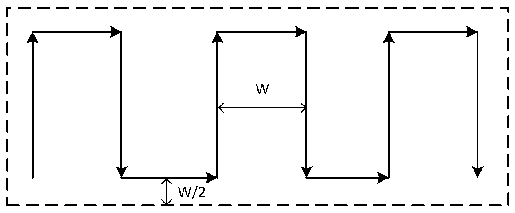
Commonly used rectangular area search methods include parallel line search and horizontal line search, as shown in Figure 2 and Figure 3.

The parallel line search method searches along the long side of the rectangle, while the horizontal line search method searches along the short side of the rectangle. These two strategies are relatively simple and will not be covered in detail in this article.

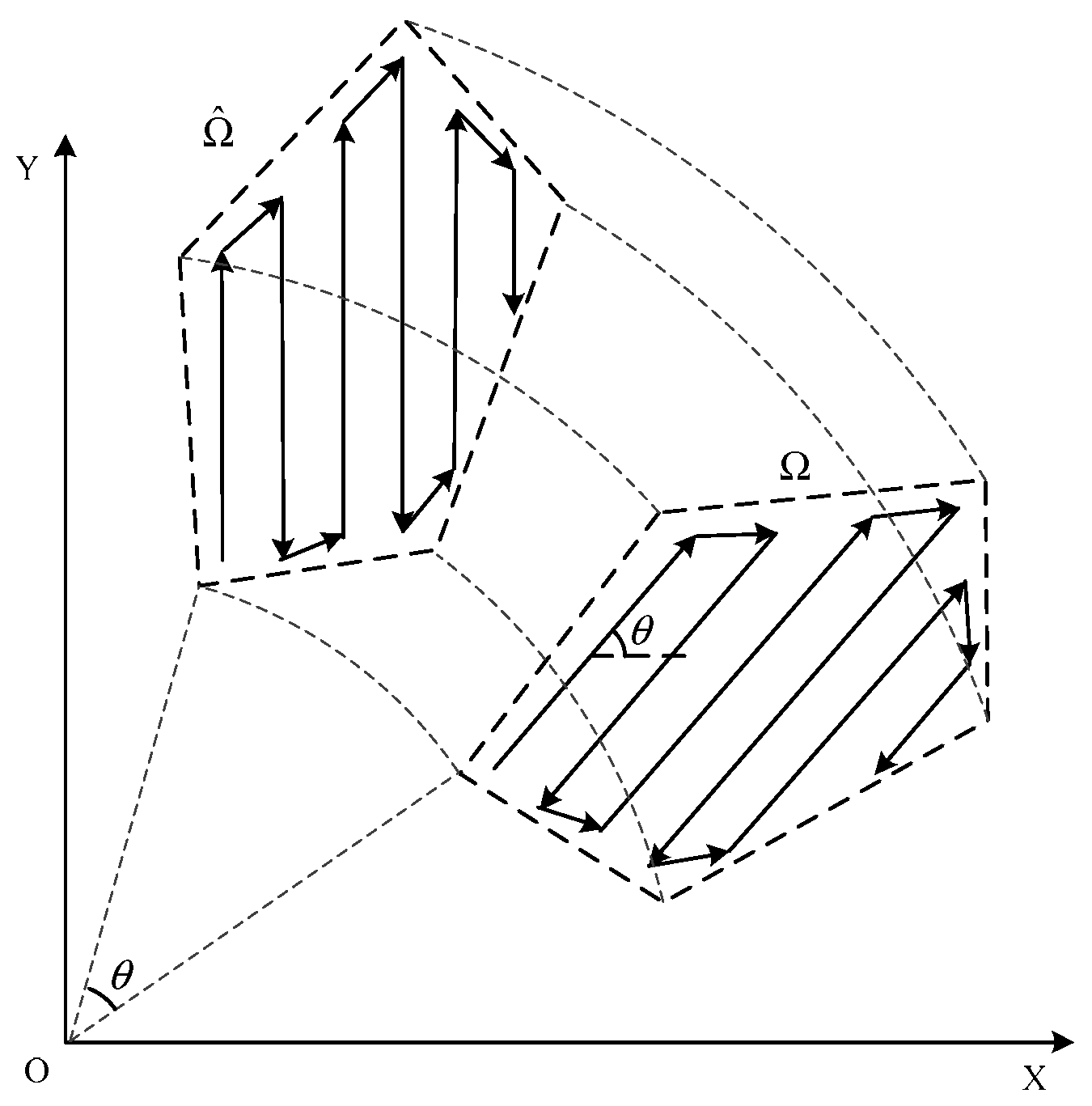
Obviously, parallel line scanning search and horizontal line search are two commonly used area search methods, but they can only be applied to rectangular areas, which is not universal enough. Therefore, this section combines the characteristics of several search methods and proposes a parallel search method with variable angles for polygonal areas, which can generate parallel search trajectories with arbitrary direction angles in any convex polygonal area. It not only covers commonly used area search methods but also provides a more flexible trajectory planning model that can generate optimal search schemes as much as possible. The algorithm principle is shown in Figure 4.

Given a convex polygon region $\mathsf{\Omega }=\left(p_1,p_2,\dots ,p_n\right)$ with n vertices, the parallel search direction angle is θ and the search line spacing is W. The planning process mainly consists of the following three steps:

Step 1—Rotate the vertices of the polygon region counterclockwise by θ to obtain a new convex polygon $\widehat{\mathsf{\Omega }}=\left({\widehat{p}}_1,{\widehat{p}}_2,\dots ,{\widehat{p}}_n\right)$. The coordinate rotation is achieved using the following rotation matrix:

$${\hat{\mathit{p}}}_i=\left[\begin{array}{cc}\cos \theta & -\sin \theta \\ \sin \theta & \cos \theta \end{array}\right]{\mathit{p}}_i$$

(5)

Step 2—Plan a parallel trajectory in the new convex polygon, with the trajectory direction parallel to the Y axis and the spacing between adjacent trajectories of W, resulting in the coordinates of the planned trajectory points being $\left({\widehat{q}}_1,{\widehat{q}}_2,\dots ,{\widehat{q}}_k\right)$.

Step 3—Rotate the planned track point clockwise by θ to obtain the parallel search track $\left(q_1,q_2,\dots ,q_k\right)$ in the original polygon area. The rotation matrix is as follows:

$${\mathit{q}}_i=\left[\begin{array}{cc}\cos \theta & \sin \theta \\ -\sin \theta & \cos \theta \end{array}\right]{\widehat{\mathit{q}}}_i$$

(6)

As can be seen from the above steps, the parallel search algorithm with variable angles mainly generates parallel tracks at arbitrary angles through coordinate rotation. This method is more convenient and more versatile. This method is also applicable to parallel line sweep search and lateral line search. Simply set the polygon area to a rectangular area, and then set the parallel search direction angle to be equal to the angle between the long side or short side.

The above process can be described as follows: when the area to be searched is an irregular polygon area, use Formula (5) to convert the area, and then obtain an area where one of the edges is parallel to the Y axis. In this way, the parallel line search method can be used to obtain the track within the transformed area. Afterwards, use Formula (6) to convert the obtained track, and then obtain the search track for the area to be searched.

The advantage of this approach is that only two transformations are required to generate a track line, ensuring that its X-axis coordinate remains relatively stable and facilitating track generation and data recording.

At the same time, minimizing the adjustment of the motion state of the drone can reduce battery consumption, allowing it to search more areas and improve search efficiency. This is also an advantage of parallel search in this article.

If the approximate location of the target is focused on a small area, the search base circle domain is usually used to determine the area to be searched. The center of the search base circle domain is the point with the highest probability of target existence, and the radius is determined according to need. Sector search, extended square search, and spiral search are all suitable for searching the search base circle domain, where sector search crosses the center multiple times, performing multiple repeated searches in the area with the highest probability of target existence, as shown in Figure 5.

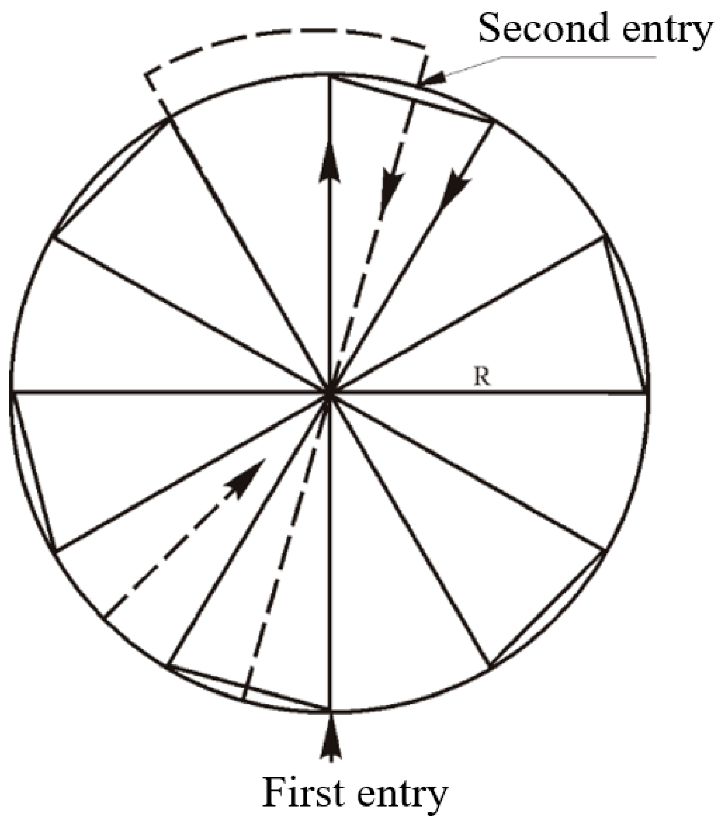
The extended square search method starts from the location with the highest probability of target presence and continuously expands outward through the extended square search method. During the secondary search, the search direction can be rotated by 45°, as shown in Figure 6.

The reason for rotating 45° during the second search is to obtain more information. For example, using three orthogonal views to observe an object can provide more comprehensive information. Therefore, for the second search, rotating 45° yields the lowest similarity to the first search trajectory, resulting in the most information gain and improved search efficiency.

The spiral search method generally uses a 20° slope to spiral, and when the spiral approaches 360°, it switches to a 15° slope; then, it spirals in turn at 10° and 5° slopes, approaching 360°, as shown in Figure 7.

3. Modeling of Search Problems

3.1. Factors That Affect Search Efficiency

3.1.1. Field of View Width

The field of view refers to the effective distance at which a drone can detect a target under specific search conditions. Targets within half the scanning width on both sides of the drone may not always be detected, but sometimes targets in more distant areas can also be detected. Accurately speaking, the probability of detecting a search target outside half the scanning width on both sides of the drone is equal to the probability of not detecting it within this distance range, as shown in Figure 8.

When a drone searches for a target through an area, it effectively searches an area with a width of W. Therefore, the sweep width is also known as the effective width, which is a good measure of the ability to detect targets.

3.1.2. Coverage Factor

The coverage factor is the ratio of the effective search range to the required search area, which describes the degree to which the required search area is thoroughly searched and can be used to measure search effectiveness or search quality. The calculation formula for the coverage factor C is as follows:

$$C=Z/A$$

(7)

where Z and A are the effective search range and the area of the required search area, respectively, or the number of grid cells contained in the probability map. For general search methods, the effective search range area Z is equal to the product of the search speed, search duration, and scan width:

$$Z=V\times T\times W$$

(8)

where V is the speed of the drone; T is the effective search time (excluding turning and other search time unrelated to effective search); and W is the sweep width. For a parallel search, the calculation of the coverage factor is relatively simple, equal to the sweep width W divided by the search line spacing S:

$$C=W/S$$

(9)

It should be noted that the concepts of sweep width and search line spacing are not the same. In fact, the setting of the search line spacing can refer to the sweep width, but it is not necessarily equal to the sweep width, and it is also related to factors such as the endurance of the drone. When the required search area is large, the endurance time of the drone cannot cover the entire area, and the value of the search line spacing should be greater than the sweep width (the coverage factor is less than 1) to ensure the search of the entire area at the expense of a certain coverage rate. When the required search area is small, the endurance time of the drone can meet the requirements, and the value of the search line spacing can be less than or equal to the sweep width (the coverage factor is greater than or equal to 1) to achieve full coverage of the search area or even cross coverage to improve the search success rate.

3.1.3. Probability of Detection

When the target is within the detection range of the search platform, the probability of correct detection is usually measured by the probability of detection (POD). If the detection device travels accurately and evaluates the search with the same width, the POD value is maximized. If the effective search width becomes narrow due to inclement weather or navigation errors, the POD value will be adversely affected.

The relationship between the POD and the coverage factor C under ideal search conditions satisfies the inverse cubic law of vision detection proved by Koopman:

$$\mathrm{POD}=erf\left(\frac{\sqrt{\pi }}{2}C\right)=erf\left(\frac{W\sqrt{\pi }}{2S}\right)$$

(10)

where erf (error function) represents the error function, and its expression is:

$$erf\left(x\right)=\frac{2}{\sqrt{\pi }}{\displaystyle \underset{0}{\overset{x}{\int }}{e}^{-t^2}dt}$$

(11)

Based on Formula (10), it can be seen that the smaller the search line spacing S, the larger the coverage factor and the higher the POD; however, a decrease in the search line spacing S will result in a reduction in the effective search area, which will decrease the POC.

At the same time, according to Formula (10), using the built-in erf function in Matlab 2021, the relationship between W and POD is plotted, as shown in Figure 9.

As can be seen in Figure 9, increasing the field of view will result in a decrease in the POD. This is also easy to understand. When other parameters remain unchanged, the larger the field of view, the lower the clarity within the field of view, which affects the detection effect of the target. However, while the detection probability increases with a smaller field of view, the search speed decreases. Therefore, the choice of the field of view also affects the search efficiency.

The increase in POD and the decrease in POC may lead to an increase or decrease in probability of success (POS); so, it is necessary to refer to the change in POS when determining the search line spacing S.

3.1.4. Probability of Success

POD only measures the conditional probability of discovering the target when it is within the search area, and it cannot measure the probability of success of the search action. However, the probability of success (POS) can truly measure the probability of success of the search action. The relationship between POS, POC, and POD is as follows:

$$\mathrm{POS}=\mathrm{POC}\times \mathrm{POD}$$

(12)

The cumulative probability of success (POS_C) is used to measure the efficiency of all search operations conducted to date. It is equal to the sum of each probability of success. In fact, after n searches, the POSC is calculated as follows:

$${\mathrm{POS}}_C{=\mathrm{POS}}_1{+\mathrm{POS}}_2+\cdots {+\mathrm{POS}}_n$$

(13)

Search operations are essentially a means of reducing the POC of search targets in an area and increasing the probability of success POS and cumulative value POSC. Within a possible area, the closer the value of POSC is to 100%, the closer the probability POC is to zero.

3.1.5. Rules for Updating the POC

During the search process, even if the target is not found, it means that the probability of the target being in that area should be appropriately reduced. Therefore, whether the target is found or not, the search information can be used to update the target’s POC in each area. The new POC value is calculated according to the following equation:

$${\mathrm{POC}}_{\mathrm{new}}=\left(1-\mathrm{POD}\right)\times {\mathrm{POC}}_{\mathrm{old}}$$

(14)

For the area not searched, the POC remains unchanged, that is, ${\mathrm{POC}}_{\mathrm{new}}={\mathrm{POC}}_{\mathrm{old}}$.

3.1.6. Probability of Detection

Suppose the number of available drone clusters is n. For the ith drone $V_i$, its parameters are known, including the location of the unmanned airport $P_i^s\left(x_i^s,y_i^s\right)$, the location of the landing airport $P_i^f\left(x_i^f,y_i^f\right)$, the maximum endurance time $T_i$, the sweep width $W_i$, the cruise speed $v_i^b$, and the search flight speed $v_i^s$. These parameters serve as inputs for search planning, and the output is all search rectangles and the search line spacing.

Each drone is responsible for a search rectangle searching task. Therefore, for each drone, a corresponding search rectangle is assigned, denoted as $Q_i\left(x_i^c,y_i^c,l_i,w_i,{\theta }_i\right)$, where $\left(x_i^c,y_i^c\right)$ is the center point coordinates of the search rectangle, $\left(l_i,w_i\right)$ are the lengths of the long and short sides of the rectangle, and ${\theta }_i$ is the direction of the long side of the rectangle. A parallel scanning search is performed in each search rectangle, with a search line spacing of $d_i$. The parameters that need to be optimized are the set of search rectangles $Q=\left(Q_1,Q_2,\dots ,Q_n\right)$ and the set of search line spacings $d=\left(d_1,d_2,\dots ,d_n\right)$.

For given a set of parameters Q and d, the cumulative probability of success can be directly calculated.

First, calculate the probability of detection POD_i for each UAV based on the search line spacing d_i and the sweep width W_i:

$${\mathrm{POD}}_i=\frac{2}{\sqrt{\pi }}{\displaystyle {\int }_0^{\frac{\sqrt{\pi }{W}_i}{2d_i}}{e}^{-t^2}dt}$$

(15)

Then, the location of the rectangle is determined based on the corresponding parameters of the search rectangle. The probabilities of the grids contained within the rectangle are added to obtain the probability of inclusion POC_i for each rectangle. The cumulative success probability is related to the optimization parameters Q and d, and is denoted as follows:

$$J\left(Q,d\right)={\displaystyle \sum _{i=1}^n{\mathrm{POC}}_i\times {\mathrm{POD}}_i}$$

(16)

When calculating the cumulative success probability, it is necessary to consider the coordination between multiple drones. According to the above calculation formula, if multiple drones perform repeated searches of the same area, they can also obtain a high cumulative success probability. To avoid such situations, it is necessary to add a POC updating mechanism. If a specific search area has already been allocated to a drone, the POC of the target probability map grid within that area is set to 0. When the drone searches again later, the cumulative success probability is not increased.

3.2. Constraint Condition

3.2.1. Time Constraints

Suppose that for drone V_i the number of waypoints in the planned search trajectory is m_i, where the coordinates of the jth waypoint are denoted as $P_i^{\left(j\right)}\left(x_i^{\left(j\right)},y_i^{\left(j\right)}\right)$. The total flight time for the drone from takeoff to landing is given by the following equation:

$$t_i=\frac{1}{v_i^b}\left(\Vert P_i^s{P}_i^{\left(1\right)}\Vert +\Vert P_i^{\left(m_i\right)}{P}_i^f\Vert \right)+\frac{1}{v_i^s}{\displaystyle \sum _{j=1}^{m_i-1}\Vert P_i^{\left(j\right)}{P}_i^{\left(j+1\right)}\Vert }$$

(17)

The first term in the above formula is the time consumed during takeoff and return, while the second term is the time consumed during the search. To ensure flight safety, a certain amount of fuel should be reserved during planning to better handle various unexpected situations. Therefore, the total flight time should not exceed 85% of the endurance time, which results in the following constraint:

$$t_i\le 0.85\times T_i$$

(18)

The above formula considers the different flight speeds of drones at different stages, and divides the search trajectory into two segments, namely, the pre-takeoff departure and return landing segments, as well as the search trajectory segment. During the pre-takeoff departure and return landing segments, drones usually use the maximum speed or cruise speed to ensure rapid arrival at the search area; during the search of the area, to meet the requirements of the search mission, drones usually maintain a lower speed. In particular, reducing the adjustment of the motion state of the drone can save the drone’s power and help improve its search efficiency.

3.2.2. Motion Constraints

Construct a coordinate system, as shown in Figure 10.

The drone flies in the mission area, which is regarded as a particle moving in three-dimensional space. Its motion equation and constraint are as follows:

$$\{\begin{array}{c}\begin{array}{c}x(k+1)=x(k)+v(k)\mathsf{\Delta }t\cos \alpha (k+1)\cos \beta (k+1)\\ \begin{array}{l}y(k+1)=y(k)+v(k)\mathsf{\Delta }t\sin \alpha (k+1)\cos \beta (k+1)\\ \begin{array}{ccc}& & \end{array}z(k+1)=z(k)+v\mathsf{\Delta }t\sin \beta (k+1)\end{array}\end{array}\\ v(k+1)=v(k)+\mathsf{\Delta }v(k)\begin{array}{cc}& v(k+1)\in \left[-v_{max},v_{max}\right]\end{array}\\ \alpha (k+1)=\alpha (k)+\mathsf{\Delta }\alpha (k)\begin{array}{cc}& \mathsf{\Delta }\alpha (k)\in \left[-\mathsf{\Delta }{\alpha }_{max},\mathsf{\Delta }{\alpha }_{max}\right]\end{array}\\ \beta (k+1)=\beta (k)+\mathsf{\Delta }\beta (k)\begin{array}{cc}& \mathsf{\Delta }\beta (k)\in \left[-\mathsf{\Delta }{\beta }_{max},\mathsf{\Delta }{\beta }_{max}\right]\end{array}\end{array}$$

(19)

In Formula (19), Δt is the time step, [x(k), y(k), z(k)] represents the spatial position of the UAV at time k, with a total of K time steps. v and Δv represent the speed and acceleration of the UAV, respectively. α and β represent the heading angle and pitch angle of the UAV. Additionally, Δα and Δβ correspond to the angular increments, respectively. v_max is the maximum speed of the UAV, and Δα_max and Δβ_max are the maximum angular changes under maneuvering performance constraints.

The motion of the drone must satisfy the above speed control and angle control constraints to ensure that the optimization results obtained are feasible.

3.2.3. Security Constraint

Safety constraints mainly include boundary constraints, no-fly zone constraints, collision avoidance constraints, and obstacle avoidance constraints.

Let the area outside the boundary be Ω_b and the no-fly zone area be Ωp. Then, the planned location of the drone at the next moment (x(k + 1), y(k + 1)) needs to satisfy the following equation:

$$\{\begin{array}{c}\left(x\left(k+1\right),y\left(k+1\right)\right)\notin {\mathsf{\Omega }}_b\\ \left(x\left(k+1\right),y\left(k+1\right)\right)\notin {\mathsf{\Omega }}_p\end{array}$$

(20)

Formula (20) is the boundary constraint and no-fly zone constraint.

Collision avoidance constraints refer to the need to ensure that the distance between the ith and jth drones during flight cannot be less than a safe distance d_s, which can prevent collisions between drones, i.e.,:

$$\{\begin{array}{c}\sqrt{{\left(x_i\left(k\right)-x_j\left(k\right)\right)}^2+{\left(y_i\left(k\right)-y_j\left(k\right)\right)}^2}\ge d_s\\ \sqrt{{\left(x_i\left(k+1\right)-x_j\left(k+1\right)\right)}^2+{\left(y_i\left(k+1\right)-y_j\left(k+1\right)\right)}^2}\ge d_s\end{array}$$

(21)

The obstacle avoidance constraint refers to the distance maintained between the drone and the mountain during flight. The threat of the mountain is generally expressed as follows:

$$f_i(x\left(k\right),y\left(k\right))=e^{-\lambda \left[\left(x\left(k\right)-x_{pi}\right)+\left(y\left(k\right)-y_{pi}\right)\right]}$$

(22)

In Formula (22), (x_pi, y_pi) represents the position coordinates of the center point of the peak of the I mountain, and λ is a parameter representing the threat distance of the peak. Then, f_i(x(k), y(k)) is the probability of a possible collision between the UAV and the peak. In addition, in the environment, in addition to the peak, the ground height is not exactly the same. Generally, it is assumed that the threat in other areas follows a two-dimensional independent Gaussian distribution.

The real environment can be simulated by superimposing the above models, as shown in Figure 11.

Then, the drone needs to meet the following requirements:

$$f_i(x\left(k\right),y\left(k\right))\le T{h}_s$$

(23)

That is, the probability of collision between the drone and the mountain is lower than the set threshold Th_s.

3.2.4. Communication Constraint

There is a need for communication between drones. However, due to the limited load capacity of drones, their communication range is also limited.

Assuming that the distance between drones i and j is D_ij and the upper limit of communication distance between drones is RC_max, the following equation should be satisfied:

$$D_{ij}\le R{C}_{\max }$$

(24)

Due to the need for drones to search as wide an area as possible but to ensure the stability of communication, the communication constraint is that for any one drone, as long as there are two other drones with a distance less than RC_max, it is considered to meet the communication constraint.

3.2.5. Communication Topology

A communication topology needs to be designed between drones to ensure the stability of communication.

The design principle of communication topology is to ensure that when any two drones lose contact with each other, data transmission can be achieved through relay communication with other drones.

Taking 5 drones as an example, this article designs a communication topology, as shown in Figure 12.

Suppose that when using topology A for communication, drones 3 and 4 lose contact with each other. At this point, it is possible to switch to topology E and use drone 1 as a communication relay to achieve communication. Topology switching is related to the lost drone. Based on the lost drone number, the corresponding switching topology is obtained, as shown in

Table 2. Topology switching table.

Unable to Communicate	Topology	Unable to Communicate	Topology
1,2	B	2,4	B
1,3	C	2,5	A
1,4	B	3,4	E
1,5	C	3,5	C
2,3	A	4,5	F

.

At this point, effective communication between drones can be guaranteed.

3.3. Search Trajectory Optimization Model

Considering the optimization objective of cumulative success probability based on search resource constraints, a nonlinear optimization model for search trajectory planning is established as follows:

$$\begin{array}{l}\max J\left(Q,d\right)=\alpha {\displaystyle \sum _{i=1}^n{\mathrm{POC}}_i\times {\mathrm{POD}}_i}-\beta \frac{1}{n}{\displaystyle \sum _{i=1}^n\frac{t_i}{0.85\times T_i}}\\ s.t.\begin{array}{cc}& t_i\le 0.85\times T_i\end{array}\end{array}$$

(25)

where α and β are weight factors. The optimization objective is divided into two parts: the first is the cumulative success probability of search, and the second is the proportion of search time to endurance time. The optimization objective is to maximize the cumulative success probability and minimize the search time. The parameters to be optimized in the above optimization problem are the search rectangle set Q and the search line spacing set d. Under the constraint of the endurance time of the UAV, the search trajectory planning scheme that maximizes the cumulative success probability J(Q, d) is solved.

The optimization problem described above is a nonlinear optimization problem with constraints, which is difficult to solve based on traditional optimization theory. Therefore, in order to facilitate optimization, this section converts the constraints into a penalty function, resulting in the following unconstrained optimization problem:

$$\left(Q^{*},d^{*}\right)=\arg \min \left[-J\left(Q,d\right)+M{\displaystyle \sum _{i=1}^n\varphi \left(t_i\right)}\right]$$

(26)

where $\varphi \left(t_i\right)-\max \left\{0,t_i-0.85\times T_i\right\}$ is the outer point penalty function, and M is the penalty factor, which is a large positive number. It should be noted that because the original optimization problem is designed to maximize in order to make the transformed problem easier to solve, a negative sign is applied to the optimization term. The optimal solution $\left(Q^{*},d^{*}\right)$ is also the optimal solution of the original optimization problem.

4. Adaptive Differential Evolution Algorithm

When there are a large number of drones, it is necessary to optimize 6n parameters, and the problem to be optimized is a high-dimensional nonlinear optimization problem. Considering the good performance of differential evolution algorithm in solving high-dimensional nonlinear optimization problems, this section improves it to optimize the search trajectory to be solved.

4.1. Differential Evolution Algorithm

Differential evolution (DE) is a heuristic search algorithm based on the theory of swarm intelligence. The main idea is to achieve the effect of overall evolution of the population through cooperation and competition among individuals within the population. The main feature of the DE algorithm is its memory mechanism, which can adaptively adjust its search strategy based on historical conditions, with stronger convergence and robustness guarantees. It is often used to solve complex optimization problems with high real-time requirements.

The evolutionary process of the basic differential evolution algorithm is divided into five steps.

Step 1: Initialization

Create a set of NP real-valued vectors with dimension D as the initial population, in which each individual is a D-dimensional vector:

$$x_{i,G}\left(i=1,2,\dots ,NP\right)$$

(27)

where G is the evolutionary generation; i represents the number of individuals in the population; and NP is the population size, which remains unchanged during the optimization process.

The initialization of the population needs to satisfy the constraints, taking random values within the upper and lower bounds. Each variable satisfies the following equation:

$$x_{ji,0}=\mathrm{rand}\left[0,1\right]\times \left(x_j^{\left(U\right)}-x_j^{\left(L\right)}\right)+x_j^{\left(L\right)},\left(j=1,2,\dots ,D\right)$$

(28)

where rand [0, 1] represents a uniform random number generated between [0, 1].

Step 2: Mutation

Mutation is achieved by calculating the difference between any two vectors:

$$v_{i,G+1}=x_{r_1,G}+F\times \left(x_{r_2,G}-x_{r_3,G}\right)$$

(29)

where r₁, r₂, and r₃ are different random numbers; F is a mutation operator that scales the difference components to avoid too small or too large a mutation. F is generally a constant.

Step 3: Crossover

The purpose of crossover is to inherit the good genes of the current population and pass them on to the new population to increase the diversity of the population. The crossover operation is as follows:

$$\begin{array}{l}\left[w_d\left(t\right),w_v\left(t\right)\right]=f\left(x,y,z,t\right)\\ u_{i,G+1}=\left(u_{1i,G+1},u_{2i,G+1},\dots u_{Di,G+1}\right)\\ u_{ji,G+1}=\{\begin{array}{c}{v}_{ji,G+1},\begin{array}{cc}if& rand\left(j\right)\le CR or j=rnbr\left(i\right)\end{array}\\ x_{ji,G+1},\begin{array}{cc}if& rand\left(j\right)>CR or j\ne rnbr\left(i\right)\end{array}\end{array}\end{array}$$

(30)

In the formula, rand(j) represents the generated random number between [0, 1] for the jth time; rnbr(i) is a randomly generated sequence that ensures that u_i,G+1 can randomly obtain a parameter; and CR is the crossover operator, which is the probability of crossover, taking values between 0 and 1.

Step 4: Handling of abnormal individuals

During the crossover and mutation processes, new individuals that do not satisfy the constraints may be generated. In this case, boundary conditions need to be applied to these individuals. To ensure the diversity of the population, abnormal individuals are directly discarded and replaced with randomly generated individuals. If the newly generated individual does not satisfy the boundary conditions, then the following equation is used:

$$u_{ji,G+1}=\mathrm{rand}\left[0,1\right]\times \left(x_j^{\left(U\right)}-x_j^{\left(L\right)}\right)+x_j^{\left(L\right)}$$

(31)

Step 5: Select

The newly generated individuals may not necessarily be able to enter the next generation population. They need to be selected through the survival of the fittest mechanism of the DE algorithm to participate in the next generation population. Therefore, through the calculation of the fitness function and comparison with the current population, only the better individuals can appear in the next generation population. Therefore, the new population inherits from the current population, and the greedy mechanism ensures that the new population is definitely better than or as good as the current population.

4.2. Adaptive Mutation Operator

In the classic DE algorithm, the mutation operator is a constant, which fixes the mutation step size. If the step size is too large, it can lead to an inaccurate search, frequent triggering of boundary conditions, and difficulty in finding the global optimal solution; if the step size is too small, it can lead to a slow search, poor population diversity, and easily falls into local optima. Therefore, the step size should be adaptively adjusted according to the optimization process of the algorithm. An adaptive mutation operator can be designed to solve this problem of a poorly determined step size.

In the process of searching for trajectory optimization, randomly generated initial solutions usually do not satisfy the constraints, and the fitness function value is high under the influence of the penalty term. The early stage of optimization is mainly to find “feasible solutions” that satisfy the constraints. It is necessary to set a large mutation operator to improve population diversity and find as many “feasible solutions” as possible to prevent the phenomenon of “premature”. The later stage of optimization is mainly to find the optimal allocation scheme in the set of “feasible solutions”. It is necessary to set a small mutation operator to improve the accuracy of the global optimal solution. Therefore, the DE algorithm with adaptive mutation operator is adopted. The adaptive mutation operator is designed as follows:

$$F=2^{\lambda }{F}_0, \lambda =e^{1-\frac{G_m}{G_m+1-G}}$$

(32)

where F₀ is a constant, which is the benchmark for the value of the mutation operator; G is the current evolution generation; and G_m is the maximum evolution generation. In the early stages of evolution, the adaptive mutation operator is 2F₀, ensuring a wide range of coarse searches and improving population diversity. As the evolution process continues, the mutation operator gradually decreases to F₀, further narrowing the scope of the precise search and improving the accuracy of the global optimal solution.

As can be seen in Formula (32), when there is no iteration, that is, G is 0, the coefficient before F₀ is 2. Using a larger mutation operator allows the iterative process to traverse the search space as much as possible. This is beneficial for tasks with strong time constraints. Namely, this method is very suitable for solving the problem of allowing the drone to search as much area as possible within a limited time.

According to Formula (25) or Formula (26), it can be seen that this paper converts the constraint condition of the time requirement into a penalty function in the objective function. This may convert some infeasible solutions into high penalty solutions, which affects the search and iteration process. In order to quickly jump out of such solutions, it is necessary to find more feasible solutions in the optimization space. Therefore, a large mutation operator is needed in the early stage.

When the algorithm enters the later stage, it needs to further fine-tune the results of feasible solutions. At this time, it is necessary to search in the vicinity of feasible solutions, rather than far away from them. Only a small mutation operator is needed to achieve micro-perturbation of parameters, resulting in a better solution.

Similarly, this method is also beneficial for planning global search problems. By traversing a large number of feasible spaces in the early stages, a better region can be obtained, followed by precise search. While improving the efficiency of optimization, it also reduces the possibility of the algorithm falling into local optima.

4.3. Variable Encoding Method

The DE algorithm combines the problem to be optimized with variable encoding. Assuming that the number of drones is n, the length of the encoding is determined to be 6n. The encoding method is shown in Figure 13.

The variable is encoded as a 6n-dimensional vector, and as the number of drones increases, the search space dimension continues to expand. When there are a large number of available drones, it is necessary to optimize search resources based on the actual search task to avoid unnecessary waste of search resources.

4.4. Steps for Solving Optimization Algorithm

The steps of the improved DE algorithm are as follows:

Step 1—Generate an initial population, with the number of generations initialized to 1. Set the population size to NP, and determine the upper and lower bounds for each variable. Randomly generate NP initial individuals that satisfy the upper and lower bound constraints.

Step 2—Calculate the fitness function. According to the encoding method, the decoding operation is reversed to obtain the search rectangle Q and search line spacing d corresponding to each UAV. The evaluation value of each individual is calculated through the fitness function.

Step 3—Evolutionary operation. Adaptively adjust the mutation operator according to the evolutionary generation, perform mutation and crossover operations on the population (satisfying the constraints), and obtain a temporary population. Perform greedy selection operations on the corresponding individuals in the temporary population and the original population, and select the winning individuals to evolve into a new population.

Step 4—Terminate optimization. Determine whether the current evolution generation has reached the maximum evolution generation or whether the termination condition has been met. If so, terminate the evolution; otherwise, return to Step 2.

4.5. Analysis of Algorithm Complexity

To further introduce the performance of the algorithm, the complexity of the algorithm is analyzed.

Compared to the classic DE algorithm, the improvement of the algorithm in this paper lies in the construction of a mutation operator and variable encoding method. The mutation operator is calculated during each iteration process. However, this value is used by every particle during the optimization process. After each iteration, it can be calculated as a constant value for that iteration. The incremental complexity of computation is minimal. At the same time, encoding is performed at the beginning stage, and using DE requires encoding the problem, so it does not affect the computational complexity

The factor that affects the computational complexity lies in the fitness function constructed in this article, which is Formula (26). According to the coding in Section 4.4, it can be seen that there are 6n parameters that need to be optimized. If calculated directly, the algorithm complexity is GNPO(n⁶). Obviously, this consumes a huge amount of computational resources. In the actual process, it is not necessary to simultaneously optimize these six parameters. It can be optimized step by step; that is, first optimize the coordinates x and y of the drone at the next moment. After determining the coordinates, optimize the length l and width w of the search area rectangle. Finally, optimize the rotation angle θ and trajectory spacing d. In this way, the algorithm complexity is reduced to GNP[O(n²) + O(n²) + O(n²)], which is convenient for algorithm solving.

5. System Model and Track Optimization Process

Based on the objective function and optimization method constructed in this article, a system model and trajectory optimization process are constructed, as shown in Figure 14.

The trajectory planning model and corresponding optimization process of the UAV cluster system constructed in this paper are shown in Figure 14.

Step 1: Initialize parameters. Initialize the task area, the position, and state parameters of the drone, and set the counting variable k = 1.

Step 2: Construct the objective function. Based on the objective function constructed in Section 3.3, calculate the corresponding process variables using Formula (26), and obtain the POSc and time constraint T.

Step 3: Construct constraints. Combine the descriptions in Section 3.2 to construct motion constraints, safety constraints, communication constraints, and communication topologies.

Step 4: Intelligent algorithm optimization. Using the improved DE algorithm, the objective function is solved under the constraints. The position of each drone at the next time is obtained. Additionally, let k = k + 1.

Step 5: Determine whether the optimization is complete. Determine whether k is less than the termination time K. If it is, it means that the optimization needs to continue, and then perform Step 6. Otherwise, perform Step 7.

Step 6: Update the status and location of the drones. Based on the output of Step 4, calculate the turning and climbing angles and speed changes, update the location and motion parameters of each drone using Formula (19), and return to Step 2 for further optimization.

Step 7: Output the optimization results. At this point, the optimization is complete and the search trajectory for each drone is output.

Through the above process, the optimization of the search trajectory of the drone cluster system can be achieved.

6. Simulation Verification

To verify the performance of the algorithm in this paper, two sets of simulation experiments are conducted in this section. They are global coverage search and time-limited search, which adjust the two coefficients in Formula (26) to achieve trajectory planning according to the task requirements.

The maximum endurance time of the UAV is T = 3 h, the sweeping width is W = 5 km, the cruising speed is v_b = 220 km/h, and the search flight speed is v_s = 180 km/h.

The parameters of the adaptive DE algorithm used to optimize the trajectory were set as follows: population size NP = 100, maximum iteration number G = 300, encoding length D = 36, initial mutation operator F₀ = 0.2, and crossover operator CR = 0.1.

6.1. Path Planning for Global Search

Suppose the search area is a 240 km × 360 km mission area. The target probability distribution has been obtained based on information such as satellites and maps, as shown in Figure 15.

The search area in Figure 15 is divided into 40 × 60 grid areas with a horizontal and vertical interval of 6 km. The color depth of the grid in Figure 15 indicates the probability of the target’s existence. The yellow grid indicates a grid with a high probability of the target’s existence, and the blue grid indicates a grid with a relatively low probability of the target’s existence.

Due to the large search area, it is difficult for a single UAV to cover the search area within a short period of time based on the search task requirements and time constraints. Assuming that there are six UAVs from two airports participating in the search, a search plan is obtained based on the search trajectory planning process using a polygon partition method, and two sets of predetermined search plans are obtained based on the trajectory optimization results using multiple partition strategies.

6.1.1. Route Planning Based on Polygon Partition Method

In this scenario, only polygonal areas are used to partition the search area and plan parallel search trajectories. Considering the sweep width and endurance, and based on the target probability distribution map, six polygonal areas are planned in the search partition, as shown in Figure 16.

In Figure 16, it is not advisable to invest too many drones in areas with low target probability of existence. Therefore, the search area is divided into larger zones and larger search line spacing is used. Correspondingly, in areas with high target probability of existence, more drones need to be invested for focused search, resulting in smaller areas and smaller search line spacing.

After completing the search partition, a drone is assigned to each partition based on the location relationship of the airport. To ensure the success rate of the search, the search line spacing and track direction angle for parallel line search of each drone are optimized using the method described in this article. The relevant parameters are shown in

Table 3. Polygonal area search route planning parameter table.

No	Spacing of Search Lines/km	Direction Angle/°
1	12	90
2	11	90
3	8.5	50
4	16	90
5	8.6	130
6	12	90

.

The planning result obtained according to the method in this article is shown in Figure 17.

As shown in Figure 17, the proposed algorithm can automatically generate parallel search tracks for any shape of polygon area, any direction angle, and any search line spacing, and can simultaneously support any number of UAVs for simultaneous task allocation and trajectory planning for multiple search areas, fully meeting the search requirements.

The search trajectory includes searching along the long side and searching along the short side, similar to the parallel sweep trajectory and the lateral sweep trajectory, but with relaxed constraints on the shape of the area, resulting in more flexible planning and more diverse options. Quantifying this search scheme, we obtain relevant parameters, as shown in

Table 4. Results of polygon search trajectory.

No.	Total Track Length/km	POD	POC	POS	POSC
1	1143.7	0.9784	0.1611	0.1576	0.9404
2	1182.5	0.9878	0.1600	0.1580
3	1220.6	0.9988	0.1233	0.1231
4	1347.7	0.9152	0.2146	0.1964
5	1210.2	0.9987	0.1288	0.1286
6	1265.8	0.9784	0.1805	0.1766

.

As can be seen from Table 4, the parallel tracks of the polygon area, due to its flexibility in area division, can basically achieve 100% area coverage during search partition, thus making the sum of the inclusion probability POC close to 100%. This is important for improving search success rate. In contrast, using only rectangles for search partition is relatively fixed and difficult to accurately partition. Search scheme one finally achieved a POS_C of 94.04%, meeting the needs of search tasks. Next, search scheme two adopts a hybrid approach of search base circle and polygon area, and then compares the advantages and disadvantages of the two schemes.

6.1.2. Route Planning Based on Multiple Strategies

According to the target probability distribution diagram, the proposed method is used to divide the region into search zones, as shown in Figure 18.

As shown in Figure 18, the proposed method plans two search base circle areas and four polygon areas. For areas with low probability of target existence, the polygon area and parallel search method are used. For areas with high probability of target existence and relatively concentrated targets, the search base circle area and extended rectangular and sector search methods are used.

Meanwhile, as shown in Figure 18, using circular regions for region division can lead to overlapping or missing parts of the region. In contrast to Figure 16, polygonal regions can better achieve full coverage of the region.

From partition 1 to partition 6, the responsible drones are numbered 1–6. The search radii for partitions 3 and 5 are 60 km and 70 km, respectively. The remaining drone trajectory planning parameters are the same as in search scheme one. Using the method proposed in this article to plan the trajectories of drones, the results are shown in Figure 19.

As shown in Figure 19, track 3 has up to 22 searches for the search base point, which is more conducive to thoroughly searching for small areas with high target probability. Track 5 actually has only one search for the search base point, but it can also achieve full coverage of the area. Moreover, track 5 starts with a limited search from a local area with high target probability, which is timely.

The corresponding indicators for this search scheme are also quantified, as shown in

Table 5. Results of multiple strategies search trajectory.

No.	Total Track Length/km	POD	POC	POS	POSC
1	745.8	0.9784	0.1030	0.1008	0.9238
2	1463.2	0.9878	0.1941	0.1917
3	2511.0	1.0000	0.1369	0.1369
4	1178.7	0.9152	0.1929	0.1766
5	2568.82	0.9999	0.1851	0.1849
6	1071.1	0.9878	0.1346	0.1330

.

As can be seen from Table 5, the POD of routes 3 and 5 can reach 1.000 and 0.999, basically achieving a thorough search of the area. However, the fan search and extended square search require longer search time. Fan search and extended square search should be used as much as possible for local areas where the probability of target existence is high. Polygon parallel search is more suitable for searching areas with a wide range of partitions and relatively low probability of target existence.

The POS_C of this solution is 92.38%, which is slightly lower than that of solution 1. The main reason is that there are some omissions during the search partition, resulting in a lower POC, which ultimately leads to a lower POS.

Through the analysis of the above two strategies, both have their advantages and disadvantages. There is a contradiction between global coverage and high coverage of key areas. In such a multi-objective optimization scenario, it is necessary to comprehensively consider the impact of various factors and the actual task requirements to obtain the optimal solution that meets the actual situation.

6.2. Track Planning for Time Limited Search

Changing the parameters before the time cost in Formula (26) can improve the algorithm’s search time requirements, thereby ensuring that more areas can be searched in the shortest possible time.

Set the search area as a 150 km × 200 km mission area and establish a target probability map. Divide the search area into 30 × 40 grid areas with a horizontal and vertical spacing of 5 km, as shown in Figure 20.

Similarly, the color intensity of the grid in Figure 20 indicates the target existence probability. The yellow grid indicates the grid with a high target existence probability, and the blue grid indicates the grid with a relatively low target existence probability. Assuming that there are two drone landing sites, each with three drones available, the landing site coordinates are (20 km, −60 km) and (120 km, −60 km).

The optimal allocation and trajectory optimization results for this search task are shown in Figure 21.

As can be seen in Figure 21, there is almost no overlap between the areas allocated to the six drones, and drones located at different takeoff and landing sites tend to choose areas closer to each other for the search, thus saving flight time. The yellow grid with a high probability of target presence has been more fully searched, while the blue grid with a low probability of target presence has been appropriately discarded due to search resource constraints.

As can be seen in Figure 21, the optimal trajectory planning method based on the adaptive differential evolution algorithm can prioritize the coverage of areas with a high probability of search target existence while satisfying the endurance time limit of the UAV, thus achieving a higher cumulative success probability.

At the same time, the search trajectory optimization results of six drones are obtained using the method proposed in this paper, as shown in

Table 6. Optimization results of search track.

No.	$\left({\mathit{x}}_{\mathit{i}}^{\mathit{c}},{\mathit{y}}_{\mathit{i}}^{\mathit{c}}\right)/\mathit{m}$	$\left({\mathit{l}}_{\mathit{i}},{\mathit{w}}_{\mathit{i}}\right)/\mathit{m}$	${\mathit{\theta }}_{\mathit{i}}/\mathit{d}\mathit{e}\mathit{g}$	${\mathit{d}}_{\mathit{i}}/\mathit{m}$
1	(73,156.7, 70,191.3)	(54,599.5, 47,520.3)	213.2	7222.5
2	(29,737.4, 46,583.9)	(84,495.5, 40,705.0)	147.7	9661.2
3	(134,605.5, 100,603.7)	(67,179.1, 41,889.8)	70.3	6601.6
4	(153,218.9, 58,636.5)	(55,627.1, 68,995.1)	221.3	8199.8
5	(37,753.8, 111,713.0)	(61,155.7, 43,792.2)	19.5	6039.9
6	(106,105.0, 29,815.4)	(53,029.2, 48,272.9)	252.7	6473.1

.

The results obtained with the method in this article are faster and more accurate, and can find the optimal allocation scheme in a larger optimization space, avoiding the subjectivity of manual formulation. When there are a large number of drones, the optimization space will also increase, resulting in increased difficulty in finding the optimal solution. The adaptive mutation operator in the adaptive differential evolution algorithm constructed in this article also helps to accelerate the convergence of the algorithm and further improve the feasibility of the scheme.

6.3. Algorithm Comparison

6.3.1. Comparison of Search Methods

To further compare the performance of the algorithms, the parameters of the UAV and simulation conditions remain unchanged, and the algorithms in this paper are compared with those in [38,39]. Each method is used to search for the region with time constraints in Section 6.1.2, and 50 simulation experiments are conducted for each method to obtain the POS of the corresponding method. The results are shown in

Table 7. Table comparing search scheme performance.

No.	Algorithm in This Paper	Algorithm in [38]	Algorithm in [39]
1	0.1469	0.1437	0.1404
2	0.1434	0.1839	0.1387
3	0.1139	0.1258	0.1390
4	0.1884	0.1718	0.1372
5	0.1171	0.1177	0.1430
6	0.1643	0.1050	0.1389
Total POS	0.8740	0.8497	0.8352

.

As shown in Table 7, the results obtained using different methods vary greatly.

The method in the literature [38] also converts the search target into a problem that achieves higher probability. Not only does it use obtaining higher probability as the objective function but it also uses Bayesian theory to infer and update the target probability, further improving the accuracy of target search and being more in line with reality. However, due to the lack of time constraints in the literature [38], the algorithm does not prioritize searching for places with higher target probabilities. If there is no time constraint, the performance of this method may be better. However, for urgent tasks, the performance of this previous method is inferior to the method in this paper.

The method in the literature [39] converts the search of a drone cluster into a process of competing with the environment, and then constructs a drone action selection strategy based on game theory to optimize the trajectory of a collaborative search. This solution approach has better theoretical support and is helpful for using classical methods to solve new problems. However, the literature [39] does not consider the situation where the target is searched but not detected during the search process. Therefore, the advantage of this method is that it can quickly search for more areas. However, the corresponding disadvantage is that due to the large search area, the quality of search is not high. Therefore, considering the probability of target detection, there is a gap between the effectiveness of this method and the method in the present paper.

6.3.2. Comparison of Optimization Methods

To reflect the performance of the optimization algorithm in this article, the algorithm in this article is compared with the classical DE algorithm, the algorithm in article [34], and the algorithm in study [40]. The comparison of the results of the fitness function during the optimization process is shown in Figure 22.

As shown in Figure 22, the proposed method is superior to the comparative method in terms of optimization performance. The method in Reference [34] uses chaos theory to improve the artificial bee colony algorithm. When the algorithm falls into local optimality, chaos theory is used to generate new solutions. The advantage of this method lies in using the theoretical chaos theory, which can almost traverse the optimization space, thus significantly improving the probability of the algorithm searching for the global optimal solution. As can be seen in Figure 22, the black solid line is almost always in a downward state, and the global optimal solution is finally found. However, as shown in Figure 22, the corresponding cost is also high, and the algorithm optimization is relatively slow.

The literature [40] uses a grouping strategy to improve the particle swarm optimization algorithm. The characteristics of its algorithm are shown in the blue curve, which is relatively obvious. This method designs multiple populations, allowing the populations to conduct a more detailed search in their respective regions. Afterwards, information exchange is conducted and the population moves towards a better region. Therefore, in the early stage, due to the lack of interaction between populations, the optimization speed of the algorithm is relatively slow. However, after the population conducts information exchange in the later stage, the optimization speed of the algorithm increases significantly. The blue curve in Figure 22 shows a direct decline. The characteristic of this method is that it searches slowly in the early stage and can quickly search for the optimal solution after information exchange in the later stage. Due to the existence of the early search mechanism, its search efficiency is slightly lower than the algorithm in this paper.

The purple curve in Figure 22 represents the classic DE method. Because its mutation operator is constant, the improved DE algorithm in this paper has a mutation operator that is twice as large as the DE mutation operator at the initial stage. This leads to the inability of the method in this paper to conduct a more in-depth search of a certain area of the optimization space, as is the case with the DE algorithm at the initial stage. Therefore, in the early stages, the fitness function decreases faster for DE compared to IDE. However, due to the constant mutation operator, it is difficult for DE to conduct a broader global search compared to IDE. As a result, it is difficult to escape from local optima after searching for local optima.

6.4. The Impact of Parameters on Algorithm Performance

6.4.1. Task Parameters

To further quantify the impact of different task parameters on search performance, this section studies the impacts of the number of drones, the width of the drone’s field of view, and the size of the search area on the search.

1.

The impact of the number of UAVs

The simulation parameters are the same as those in the previous section. The search results for different numbers of drones are calculated, and a comparison of the results is shown in

Table 8. The influence of different numbers of drones on the search results.

Number of UAVs	POS	Increment of POS
4	0.6156
5	0.7673	0.1517
6	0.8740	0.1067
7	0.9172	0.0432
8	0.9394	0.0222

.

As can be seen in Table 8, there is clearly no linear relationship between the POS and the number of drones. As shown in Figure 21 in the previous article, when six drones are dispatched, the search success rate of 87.4% of the mission area is basically achieved. Due to the high POS at this time, the remaining areas are scattered and the POD is not high. Increasing the number of drones does not help much to improve the search efficiency. However, on the contrary, if the number of drones is reduced, the value of POS will be significantly reduced. Because at this time the drone task is full. Reducing the number of drones will lead to some high-value areas being unable to be searched. Moreover, as the number of drones decreases, the impact on POS will become greater and greater.

From this, it can be concluded that when the POS is large, increasing the number of drones does not significantly improve search efficiency, but reducing the number of drones is not recommended. Conversely, when the POS is small, the number of drones should be increased, which has a good effect on improving the search efficiency.

2.

The impact of the field of view width

To further explore the impact of the UAV field of view width W on the search efficiency, the W value during the previous simulation process was set as the standard. The search field of view was changed by multiplying it by a factor ranging from 0.6 to 1.4, resulting in a relationship between W and POS, as shown in Figure 23.

As can be seen in Figure 23, when W takes values in the certain range, the POS will be higher. However, taking too large or too small W will affect the search performance. When W is small, the UAV’s field of view is small, and the search efficiency is significantly reduced. When W is large, although the UAV’s field of view is larger, the detection probability, or POD, decreases, resulting in a decrease in the POS. However, this decrease is not as significant as the decrease in the field of view.

Through simulation, it can be concluded that there is an ideal range of values for W during the search process of the UAV. When it deviates from this range, the search efficiency of the UAV will decrease.

3.

The impact of the size of the search area

To further explore the impact of the task area size on search performance, the task area in Figure 20 was used as a standard, and its length and width were multiplied by a factor of 0.5 to 1.5 at same time to change the size of the task area. Similarly, the relationship between the multiplier and POS was obtained, as shown in Figure 24.

As can be seen in Figure 24, the size of the task area is positively correlated with the POS. At this time, the drone can better complete the search in the area. Therefore, when the task area changes slightly, it has little impact on the POS. When the task area becomes smaller, the drone search area takes up a larger proportion, and the POS gradually approaches one. However, as the task area continues to increase, the POS decreases significantly. At this time, the drone cannot search the task area with high coverage, and can only search high-value areas as soon as possible. Therefore, the value of POS is very low.

It can also be concluded that when the drone can search the task area significantly, appropriately adjusting the increase or decrease in the task area has a low impact on the overall search efficiency. However, when the drone cannot perform a good search of the task area, it should be supplemented to perform the search of the task area, thereby improving the search efficiency.

At the same time, when the task area increases, the impact on the amount of computation is also greater. Although the algorithm complexity does not change during a single iteration, it is still O(3n²). However, as the optimization space of the algorithm increases in a quadratic form, it is necessary to increase the number of iterations G or the population size NP. Through experimental testing, it is recommended that both of these increments also be quadratic. That is, when the length and width are increased by a factor of two, G or NP or the product of both should be at least four times the original value. This results in a fourfold increase in computation.

6.4.2. Comparison of Search Methods

To further investigate the impact of algorithm parameters on search performance, this section analyzes the impacts of iteration times and population size on optimization through experiments.

1.

The impact of iterations

To investigate the effect of the number of iterations on the results, we set the number of iterations to 230, 270, and 300, respectively, and obtained the relationship between the number of iterations and the fitness function, as shown in Figure 25.

As can be seen in Figure 25, when the number of iterations is reduced, the impact on the proposed method is strong. This is because the improved mutation operator in this paper is related to the number of iterations of the algorithm. When the number of iterations is small, the proportion of the number of iterations already iterated to the total number of iterations changes rapidly, making it difficult for the mutation operator to play its role. At this point, the performance of the algorithm significantly decreases and even approaches that of classical DE algorithms.

Therefore, in order to ensure the performance of the algorithm, sufficient iterations are required. This not only ensures the effectiveness of the algorithm but also facilitates the search for the global optimum.

2.

The impact of the population size

To study the impact of population size on algorithm performance, the population size of NP = 100 described earlier was used as a standard, and population sizes of 1.5NP and 2NP were set. Through experiments, the relationship between NP and the fitness function was obtained, as shown in Figure 26.

As can be seen in Figure 26, when the population size increases, the optimization effect of the algorithm significantly improves. Especially when the population size doubles, the fitness function decreases significantly. This is because there are more particles participating in the optimization, which has a significant impact on search performance.

However, the increase in NP corresponds to an increase in the amount of computation. Although there is a linear relationship between NP and the total amount of computation, the total amount of computation is GNP[O(3n²)]. For every increase in NP, the total amount of computation increases by G[O(3n²)].

Therefore, when computing power is limited, it is necessary to weigh the relationship between computation and the task time in order to maximize the search efficiency.

7. Conclusions

This article comprehensively considers the influence and constraints of various factors and designs a search method for the task area using a drone cluster. This article constructs a search area allocation strategy based on the average inclusion probability and proposes new search models, such as polygons, sectors, and expanded rectangles, as well as corresponding trajectory optimization strategies. At the same time, with the maximization of the probability of success as the optimization goal, a constrained search trajectory optimization model is established. The differential evolution algorithm is improved to solve the model and obtain the search trajectory of the drone. The research results have positive significance for solving the collaborative search problem of drone clusters.

To improve and optimize the search method, further research on the optimization method of locating points in irregular polygonal areas can be conducted in the future, which will further enhance the practicality of the algorithm. At the same time, when the UAV has searched an area, its target probability will be updated, and a secondary search strategy can be designed based on the updated results. Setting the parameters of the optimization algorithm according to the problem to be optimized can also help improve the performance of the algorithm. An in-depth study of these contents plays a good role in improving the efficiency of collaborative search.

References

1. Alotaibi, E.T.; Alqefari, S.S.; Koubaa, A. LSAR: Multi-UAV Collaboration for Search and Rescue Missions. IEEE Access 2019, 7, 55817–55832. [Google Scholar] [CrossRef]
2. Huang, H.; Yang, Y.; Wang, H.; Ding, Z.; Sari, H.; Adachi, F. Deep Reinforcement Learning for UAV Navigation Through Massive MIMO Technique. IEEE Trans. Veh. Technol. 2020, 69, 1117–1121. [Google Scholar] [CrossRef]
3. Brown, A.; Anderson, D. Trajectory Optimization for High-Altitude Long-Endurance UAV Maritime Radar Surveillance. IEEE Trans. Aerosp. Electron. Syst. 2020, 56, 2406–2421. [Google Scholar] [CrossRef]
4. Liu, L.; Qu, G.; Kong, W. UAV 3D trajectory planning by using dynamic programming and potential theory. Comput. Eng. Appl. 2013, 49, 235–239. [Google Scholar]
5. Nie, S.; Wang, C.; Xi, X.; Luo, S.; Li, G.; Cheng, F. A Continuous Wavelet Transform Based Method for Ground Elevation Estimation Over Mountainous Vegetated Areas Using Satellite Laser Altimetry. IEEE J. Sel. Top. Appl. Earth Obs. Remote Sens. 2018, 11, 2945–2956. [Google Scholar] [CrossRef]
6. Chen, X.; Zhang, B.; Cen, M.; Guo, H.; Zhang, T.; Zhao, C. SRTM DEM-Aided Mapping Satellite-1 Image Geopositioning without Ground Control Points. IEEE Geosci. Remote Sens. Lett. 2017, 14, 2137–2141. [Google Scholar] [CrossRef]
7. Nicola, C.; Mauro, D.M.; Andrea, G. Antonio Giannitrapani, Antonio Vicino. Path Planning with Uncertainty: A Set Membership Approach. Int. J. Adapt. Control Process. 2011, 25, 273–287. [Google Scholar]
8. Zhang, K.; Zhou, D.; Yang, Z.; Kong, W.; Zeng, L. A Novel Heterogeneous Sensor-Weapon-Target Cooperative Assignment for Ground-to-Air Defense by Efficient Evolutionary Approaches. IEEE Access 2020, 8, 227373–227398. [Google Scholar] [CrossRef]
9. Wen, N.; Zhao, L.; Su, X.; Ma, P. UAV online path planning algorithm in a low altitude dangerous environment. IEEE/CAA J. Autom. Sin. 2015, 2, 173–185. [Google Scholar] [CrossRef]
10. Lu, Y.; Lei, X.; Zhou, Z.; Song, Y. Approximate Reasoning Based on IFRS and DS Theory With its Application in Threat Assessment. IEEE Access 2020, 8, 160558–160568. [Google Scholar] [CrossRef]
11. Golestan, K.; Khaleghi, B.; Karray, F.; Kamel, M.S. Attention Assist: A High-Level Information Fusion Framework for Situation and Threat Assessment. IEEE Trans. Intell. Transp. Syst. 2016, 17, 1271–1285. [Google Scholar] [CrossRef]
12. Zhang, Q.; Zhou, C.; Tian, Y.; Xiong, N.; Qin, Y.; Hu, B. A Fuzzy Probability Bayesian Network Approach for Dynamic Cybersecurity Risk Assessment in Industrial Control Systems. IEEE Trans. Ind. Inform. 2018, 14, 2497–2506. [Google Scholar] [CrossRef]
13. Sujit, P.B.; Ghose, D. Search using multiple UAVs with flight time constraints. IEEE Trans. Aerosp. Electron. Syst. 2004, 40, 491–509. [Google Scholar] [CrossRef]
14. Nair, R.R.; Behera, L.; Kumar, V.; Jamshidi, M. Multisatellite Formation Control for Remote Sensing Applications Using Artificial Potential Field and Adaptive Fuzzy Sliding Mode Control. IEEE Syst. J. 2015, 9, 508–518. [Google Scholar] [CrossRef]
15. Wai, R.; Prasetia, A.S. Adaptive Neural Network Control and Optimal Path Planning of UAV Surveillance System with Energy Consumption Prediction. IEEE Access 2019, 7, 126137–126153. [Google Scholar] [CrossRef]
16. Huang, C.; Lv, C.; Hang, P.; Xing, Y. Toward Safe and Personalized Autonomous Driving: Decision-Making and Motion Control with DPF and CDT Techniques. IEEE/ASME Trans. Mechatron. 2021, 26, 611–620. [Google Scholar] [CrossRef]
17. Li, X.; Li, X.; Ge, S.S.; Khyam, M.O.; Luo, C. Automatic Welding Seam Tracking and Identification. IEEE Trans. Ind. Electron. 2017, 64, 7261–7271. [Google Scholar] [CrossRef]
18. Zhu, D.-D.; Sun, J.-Q. A New Algorithm Based on Dijkstra for Vehicle Path Planning Considering Intersection Attribute. IEEE Access 2021, 9, 19761–19775. [Google Scholar] [CrossRef]
19. Luo, M.; Hou, X.; Yang, J. Surface Optimal Path Planning Using an Extended Dijkstra Algorithm. IEEE Access 2020, 8, 147827–147838. [Google Scholar] [CrossRef]
20. Orozco-Rosas, U.; Montiel, O.; Sepúlveda, R. Mobile robot path planning using membrane evolutionary artificial potential field. Appl. Soft Comput. 2019, 77, 236251. [Google Scholar] [CrossRef]
21. Yao, Q.; Zheng, Z.; Qi, L.; Yuan, H.; Guo, X.; Zhao, M.; Liu, Z.; Yang, T. Path Planning Method with Improved Artificial Potential Field—A Reinforcement Learning Perspective. IEEE Access 2020, 8, 135513–135523. [Google Scholar] [CrossRef]
22. Mclain, T.; Beard, R. Trajectory planning for coordinated rendezvous of unmanned air vehicles. Fire Control Command Control 2009, 34, 1247–1254. [Google Scholar]
23. Shanmugavel, M.; Tsourdos, A.; White, B.; Żbikowski, R. Co-operative path planning of multiple UAVs using Dubins paths with clothoid arcs. Control Eng. Pract. 2010, 18, 1084–1092. [Google Scholar] [CrossRef]
24. Ari, I.; Aksakalli, V.; Aydogdu, V.; Kum, S. Optimal ship navigation with safety distance and realistic turn constraints. Eur. J. Oper. Res. 2013, 229, 707–717. [Google Scholar] [CrossRef]
25. Wen, Q.; Xia, Q.; Su, W. Bank-to-Turn Guidance Law with Terminal Impact-Angle Constraint. J. Aerosp. Eng. 2016, 29, 04015067. [Google Scholar]
26. Zhang, Q.; Wang, Z.; Tao, F. Optimal guidance law design for impact with terminal angle of attack constraint. Opt. Int. J. Light Electron Opt. 2014, 125, 243–251. [Google Scholar] [CrossRef]
27. Zhen, L.; Liu, Y.; Dongsheng, W.; Wei, Z. Parameter Estimation of Software Reliability Model and Prediction Based on Hybrid Wolf Pack Algorithm and Particle Swarm Optimization. IEEE Access 2020, 8, 29354–29369. [Google Scholar] [CrossRef]
28. Chen, Y.; Yang, D.; Yu, J. Multi-UAV Task Assignment with Parameter and Time-Sensitive Uncertainties Using Modified Two-Part Wolf Pack Search Algorithm. IEEE Trans. Aerosp. Electron. Syst. 2018, 54, 2853–2872. [Google Scholar] [CrossRef]
29. Alb, M.; Alotto, P.; Magele, C.; Renhart, W.; Preis, K.; Trapp, B. Firefly Algorithm for Finding Optimal Shapes of Electromagnetic Devices. IEEE Trans. Magn. 2016, 52, 7002504. [Google Scholar] [CrossRef]
30. Slowik, A.; Kwasnicka, H. Nature Inspired Methods and Their Industry Applications—Swarm Intelligence Algorithms. IEEE Trans. Ind. Inform. 2018, 14, 1004–1015. [Google Scholar] [CrossRef]
31. Tang, L.; Tian, C.; Xu, K. Exploiting Quality-Guided Adaptive Optimization for Fusing Multimodal Medical Images. IEEE Access 2019, 7, 96048–96059. [Google Scholar] [CrossRef]
32. Iscan, H.; Kiran, M.S.; Gunduz, M. A Novel Candidate Solution Generation Strategy for Fruit Fly Optimizer. IEEE Access 2019, 7, 130903–130921. [Google Scholar] [CrossRef]
33. Su, F.; Li, Y.; Shen, L. An Improved Ant Colony Algorithm for UAV Route Planning in Complex Battlefield Environment. In Proceedings of the 2009 Chinese Control and Decision Conference, Guilin, China, 17–19 June 2009; pp. 3568–3573. [Google Scholar]
34. Xu, C.; Duan, H.; Liu, F. Chaotic artificial bee colony approach to uninhabited combat air vehicle (UCAV) path planning. Aerosp. Sci. Technol. 2010, 14, 535–541. [Google Scholar] [CrossRef]
35. Fu, Y.; Ding, M.; Zhou, C. Phase angle-encoded and quantum-behaved particle swarm optimization applied to three-dimensional route planning for UAV. IEEE Trans. Syst. Man Cybern. Part A 2012, 42, 511–526. [Google Scholar] [CrossRef]
36. Roberge, V.; Tarbouchi, M.; Labonté, G. Comparison of Parallel Genetic Algorithm and Particle Swarm Optimization for Real-Time UAV Path Planning. IEEE Trans. Ind. Inform. 2013, 9, 132–141. [Google Scholar] [CrossRef]
37. Song, Q.; Zhao, Q.; Wang, S.; Liu, Q.; Chen, X. Dynamic Path Planning for Un-manned Vehicles Based on Fuzzy Logic and Improved Ant Colony Optimiza-tion. IEEE Access 2020, 8, 62107–62115. [Google Scholar] [CrossRef]
38. Ni, J.; Tang, G.; Mo, Z.; Cao, W.; Yang, S.X. An Improved Potential Game Theory Based Method for Multi-UAV Cooperative Search. IEEE Access 2020, 8, 47787–47796. [Google Scholar] [CrossRef]
39. Saadaoui, H.; Bouanani, F.E.; Illi, E. Information Sharing Based on Local PSO for UAVs Cooperative Search of Moved Targets. IEEE Access 2021, 9, 134998–135011. [Google Scholar] [CrossRef]
40. Hao, L.; Xiangyu, F.; Manhong, S. Research on the Cooperative Passive Location of Moving Targets Based on Improved Par-ticle Swarm Optimization. Drones 2023, 7, 264. [Google Scholar] [CrossRef]
Figure 1. Comparison of different types of search areas.
Drones 08 00132 g001
Figure 2. Parallel line search.
Drones 08 00132 g002
Figure 3. Horizontal line search.
Drones 08 00132 g003
Figure 4. Parallel search algorithm based on variable angles.
Drones 08 00132 g004
Figure 5. Fan-shaped search diagram.
Drones 08 00132 g005
Figure 6. Extended square diagram.
Drones 08 00132 g006
Figure 7. Spiral search method diagram.
Drones 08 00132 g007
Figure 8. Field of view width diagram.
Drones 08 00132 g008
Figure 9. Relationship between the field of view width and POD.
Drones 08 00132 g009
Figure 10. UAV coordinate system.
Drones 08 00132 g010
Figure 11. Simulation diagram of a mountain threat.
Drones 08 00132 g011
Figure 12. Communication topology. (a) Topology A. (b) Topology B. (c) Topology C. (d) Topology D. (e) Topology E. (f) Topology F.
Drones 08 00132 g012
Figure 13. Schematic diagram of DE algorithm encoding.
Drones 08 00132 g013
Figure 14. System model and algorithm flowchart.
Drones 08 00132 g014
Figure 15. Search area and target probability distribution diagram.
Drones 08 00132 g015
Figure 16. Polygon search partition plan.
Drones 08 00132 g016
Figure 17. Polygon search trajectory planning diagram.
Drones 08 00132 g017
Figure 18. Partition map based on multiple strategy partitioning.
Drones 08 00132 g018
Figure 19. Multiple strategies search trajectory planning diagram.
Drones 08 00132 g019
Figure 20. Probability distribution diagram of targets in the search area.
Drones 08 00132 g020
Figure 21. Search area allocation and track planning results.
Drones 08 00132 g021
Figure 22. Chart comparing optimization algorithms.
Drones 08 00132 g022
Figure 23. Relationship between W and POS.
Drones 08 00132 g023
Figure 24. Diagram of the relationship between the task area size and the POS.
Drones 08 00132 g024
Figure 25. Diagram of the relationship between the iterations and the POS.
Drones 08 00132 g025
Figure 26. Diagram of the relationship between the population size and the POS.
Drones 08 00132 g026