Abstract
A proposed strategy for managing airspace and preventing illegal drones from compromising security involves the use of autonomous drones equipped with three key functionalities. Firstly, the implementation of YOLO-v5 technology allows for the identification of illegal drones and the establishment of a visual-servo system to determine their relative position to the autonomous drone. Secondly, an extended Kalman filter algorithm predicts the flight trajectory of illegal drones, enabling the autonomous drone to compensate in advance and significantly enhance the capture success rate. Lastly, to ensure system robustness and suppress interference from illegal drones, an adaptive fast nonsingular terminal sliding mode technique is employed. This technique achieves finite time convergence of the system state and utilizes delay estimation technology for the real-time compensation of unknown disturbances. The stability of the closed-loop system is confirmed through Lyapunov theory, and a model-based hardware-in-the-loop simulation strategy is adopted to streamline system development and improve efficiency. Experimental results demonstrate that the designed autonomous drone accurately predicts the trajectory of illegal drones, effectively captures them using a robotic arm, and maintains stable flight throughout the process.
1. Introduction
Rotor drones [1], known for their vertical takeoff and landing capabilities, exceptional stability during hovering, agile flight maneuvers, and ease of control, have found widespread applications in aerial photography, mapping, logistics, and search and rescue operations [2]. However, the affordability and accessibility of rotor drones have led to a proliferation of illegal usage driven by curiosity, invasion of privacy, commercial interests, or political motives [3]. Illegal drones pose a grave threat by infringing upon personal privacy and disrupting social order. Existing measures for managing airspace primarily rely on radio frequency jammers and similar devices to interfere with and neutralize illegal drones [4]. Nevertheless, the effectiveness of radio frequency jammers is limited due to their shorter range and inability to detect autonomous drones, resulting in decreased efficiency in congested radio frequency areas [5]. Moreover, using radio frequency jammers in densely populated regions is unsuitable as it may endanger ground personnel when the illegal drones plummet to the ground [6]. Therefore, the most viable approach to combatting illegal drones lies in autonomously identifying, tracking, and capturing them, while ensuring a stable flight state and transporting them to secure zones. Considering the high mobility characteristic of illegal drones [7] and maintaining stable flight conditions during the identification, tracking, and capture process poses a formidable challenge.
In recent years, there has been a widespread application of intelligent perception components such as cameras [8], millimeter-wave radar [9], and LIDAR [10] in mobile robots. By incorporating cameras with deep learning-based object detection algorithms like YOLO (You Only Look Once) [11], SSD (Single Shot MultiBox Detector) [12], and RetinaNet [13], these robots have demonstrated exceptional recognition capabilities for shapes and colors, enabling the accurate tracking of illegal unmanned aerial vehicles (drones). Cameras, with their lightweight and compact design, do not compromise the payload capacity of autonomous drones [14]. When compared to millimeter-wave radar and LIDAR, cameras are the most suitable choice for identifying illegal drones.
Visual servoing applies visual sensors to acquire real-time image information and utilizes these data to accomplish objectives such as target tracking, localization and navigation, posture control, and feedback control [15]. This technology enables the precise positioning, path planning, posture adjustment, and autonomous control of robots [16]. Visual servoing encompasses Position-based Visual Servoing (PBVS) and Image-based Visual Servoing (IBVS) [17]. PBVS involves establishing a mapping relationship between the autonomous drone and the target drone in relation to the inertial coordinate system [18], requiring GPS information. However, commercial GPS information has a positioning error of up to 1 m, which is larger than the size of the target drones. On the other hand, IBVS directly defines image plane coordinates using image features, rather than task space [19]. Its fundamental principle involves calculating control variables from the error signal and converting them into the motion space of the autonomous drone. By employing the obtained image error for closed-loop feedback control, the autonomous drone can move towards the target drone and accomplish the tracking process.
Considering the maneuverability of illegal drones, if the position of the illegal drone in the next moment can be predicted in advance during the tracking process, it would be beneficial for the trajectory planning [20] of the autonomous drone, allowing it to reach the capture position earlier and improve capture efficiency. Currently, trajectory prediction methods mainly include interpolation methods, linear regression, filtering methods, dynamic model methods, and machine learning methods [21]. The position signal of the illegal drone obtained using computer vision techniques contains noise [22]. Interpolation methods are sensitive to noisy data or outliers, resulting in prediction deviations. In addition, interpolation methods are usually based on linear or polynomial interpolation principles, making it difficult to reflect complex nonlinear relationships. Linear regression models have a trade-off between bias and variance. When the model complexity is insufficient, underfitting may occur, meaning the model fails to fit the data well. On the other hand, when the model complexity is too high, overfitting may occur, whereby the model performs well on the training data but poorly on new data. Dynamic model methods and machine learning methods both involve solving complex mathematical optimization problems, especially for nonlinear and non-convex problems, which can be time-consuming. Filtering methods mainly include Kalman filtering [23], particle filtering, etc. Among them, the Extended Kalman Filter (EKF) algorithm [24], which is an extension of the KF algorithm, can be used for nonlinear models, and is highly acclaimed for its low computational complexity and fewer computational resource requirements. It provides a feasible solution for real-time and efficient state estimation and trajectory prediction.
Configuring an automatically triggered robotic arm beneath the autonomous drone, which closes and grasps the unauthorized drone upon catching up with it, is crucial. However, during this process, the autonomous drone is susceptible to strong interference, which can potentially lead to a crash. Enhancing the robustness of the system is vital to mitigate the risk of a crash. The real-time estimation of external disturbances and compensation for unknown disturbances are key challenges in achieving stable flight for autonomous drones. Time Delay Estimation Control (TDC) is a nonlinear control strategy that effectively addresses unknown disturbances in dynamic control problems with complex nonlinear effects [25]. TDC utilizes the previous state of the system to estimate the current collective dynamics. It offers a concise and efficient model-free control strategy. TDC is suitable for handling continuous and slow-varying unknown disturbances [26]. However, when impact signals exist within the system, the control effectiveness of TDC can be weakened. Therefore, combining TDC with other robust control algorithms can compensate for estimation errors and enhance the robustness of the control system.
Sliding mode control is a robust, fast-response, and simple implementation nonlinear control strategy [27]. It suppresses system parameter disturbances and external disturbances by introducing sliding manifolds and quickly responds to changes in system states [28]. With advances in sliding mode control theory [29], Fast Non-Singular Terminal Sliding Mode Control (FNTSM) has emerged in recent years [30]. It achieves the finite-time convergence of system states and improves control robustness. Therefore, for a class of underactuated drone systems containing time-varying uncertain nonlinearities, unknown, and impulsive disturbances, the complex external disturbances are generalized as an aggregated unknown term. Based on Terminal Sliding Mode Control (TSMC), FNTSM is introduced to construct a composite controller. The traditional PD-type sliding manifold is upgraded to a PID-type sliding manifold, which obtains faster transient response and smaller steady-state error through the integral term [31]. Furthermore, to avoid the drawback of fixed high gain coefficients that may lead to system oscillations and trigger high-frequency unmodeled terms, a parameter adaptive updating mechanism is introduced into the PID-type sliding manifold to achieve the adaptive tuning of control parameters. The derivative of the control gain is proportional to the sliding manifold, which is beneficial for suppressing the adverse effects of noise. Without changing the structure of the sliding manifold, the increase in gain automatically adjusts with the change of the sliding manifold and accelerates convergence speed when the sliding variable deviates from the sliding manifold.
The contributions of this work can be further emphasized as follows: (1) In order to suppress the interference of illegal drones on autonomous drones and maintain stable flight, sliding mode control is introduced into Target Drone Control (TDC), forming a new robust control strategy integrating adaptive PID-type sliding manifold, TDC, and fast non-singular terminal sliding mode, which has strong robustness and characteristics of model-free control. (2) In order to reach the capture position in advance and improve capture efficiency, the EKF algorithm is integrated into IBVS to estimate the future position of the target drone, providing feasible solutions for real-time and efficient state estimation and trajectory prediction. The superiority of the proposed methods is verified through counter drone capture experiments.
The remaining parts of this paper are organized as follows: Section 2 presents the system design, including the modeling of the counter drone dynamics, IBVS method, EKF trajectory prediction, and controller design. Section 3 presents hardware-in-the-loop simulation and flight experiments. Section 4 concludes the paper.
2. System Design
The system diagram in Figure 1 depicts the remote communication between the ground station and the counter drone, which is equipped with an onboard computer featuring autonomous flight capabilities and intelligent perception using a camera to detect the illegal drone. The proposed airspace management strategy incorporates three critical technologies: IBVS, a trajectory prediction module based on the EKF, and a non-linear robust controller.
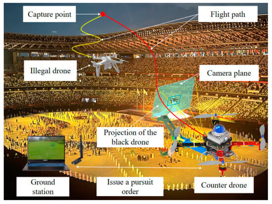
Figure 1.
Schematic diagram of the capture process of counter drone.
The core idea of the counter capture strategy is to integrate IBVS and EKF algorithms to estimate the future position of the illegal drone. The mechanical arm is then used to capture the target at a specified velocity, ultimately bringing the illegal drone to a designated area. Subsequently, key issues such as the dynamic modeling of the counter drone, IBVS, and trajectory prediction will be discussed.
2.1. Counter Drone Dynamics Modeling
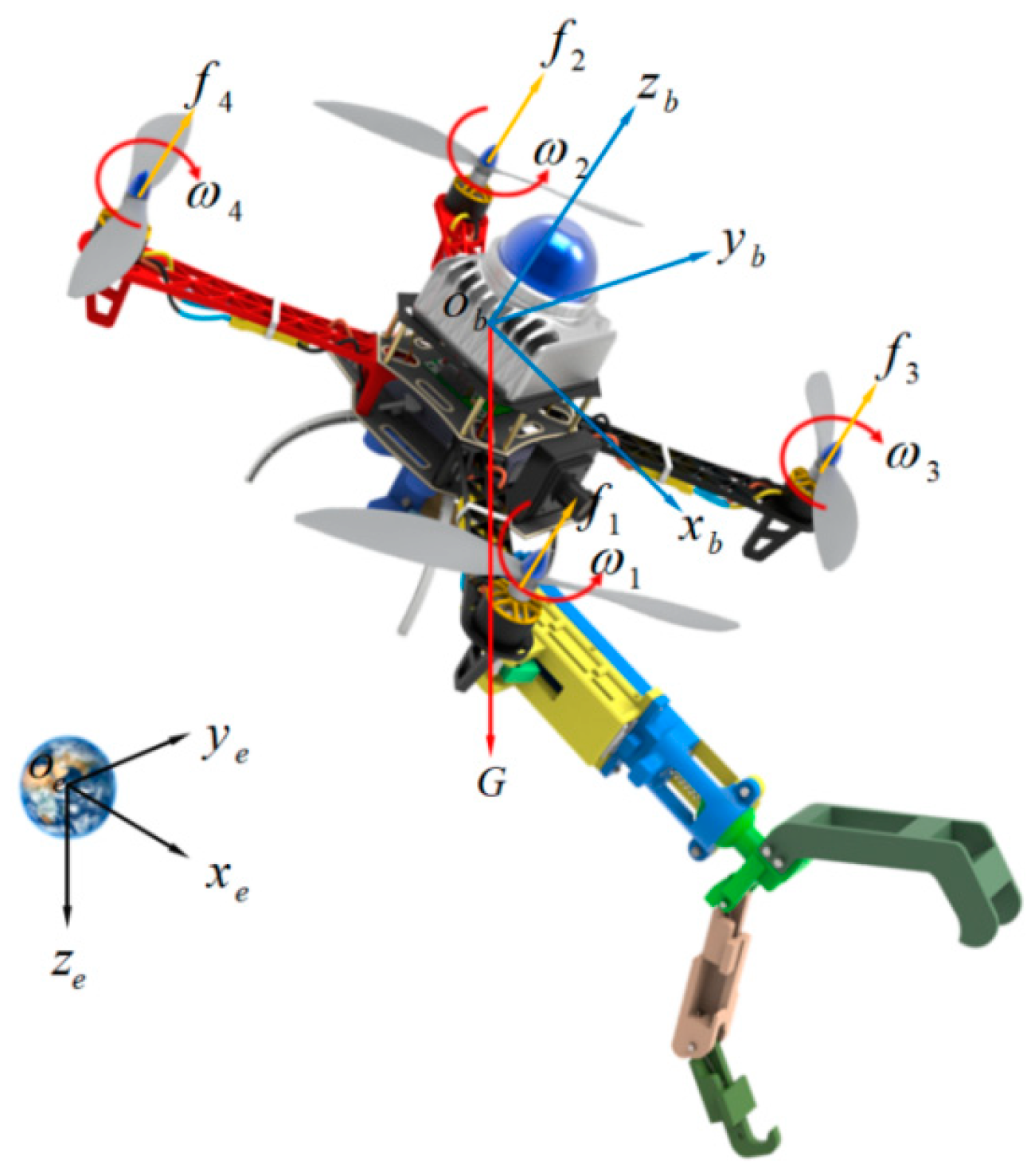
The dynamics model of the drone is utilized for designing robust controllers. The counter drone is a quadcopter, which is a nonlinear, underactuated, and strongly coupled dynamic system with four input control signals and six output states. As shown in Figure 2, the counter drone is considered as a rigid body model, experiencing the lift generated by four motors and its own weight, with three position coordinates and three attitude angles. The figure depicts the world coordinate system denoted as {e} and the body coordinate system denoted as {b}.

Figure 2.
Force diagram of counter drone.
The counter drone dynamics model consists of both position dynamics and attitude dynamics models, with the position dynamics model encompassing horizontal and vertical channel dynamics models [32].
The horizontal channel dynamics model is established based on the Newton–Euler dynamics theory [33]:
where represents the horizontal acceleration in the world coordinate system; X and Y represent the positions in the xe and ye directions under the world coordinate system, respectively; and represent the speeds in the xe and ye directions in the world coordinate system, respectively; ; ; represents the yaw angle; represents the roll angle; represents the pitch angle; represents the horizontal disturbance.
The dynamic model of the vertical channel is established as follows:
where is the total thrust of the drone; , , and are the displacements, velocities, and accelerations in the z direction in the world coordinate system, respectively; m is the total mass of the drone; g is the acceleration of gravity; l is the drag coefficient; and ΔP is the mechanical hand dynamics term.
We define as follows:
where can be considered as a lumped uncertainty term that includes counter drone gravity, torque, manipulator dynamics, and external disturbances. Then the above formula can be changed to:
The following content is the posture dynamics model
where represents the torque of the propeller relative to the body axis; denotes the rotational inertia about the three axes of the counter drone; corresponds to the angular velocity in the body coordinate system; stands for the angular acceleration in the body coordinate system; and signifies the gyroscopic torque experienced by the drone.
Based on the small perturbation assumption, we obtain
where .
2.2. Image-Based Visual Servoing Method
During the theoretical analysis phase, two fundamental assumptions are provided.
Assumption 1:
The relative position between the counter drone’s body coordinate system and the camera coordinate system remains constant.
Rotation matrix
Assumption 2:
The counter drone can record in real time the center coordinates of the illegal drone, which are acquired via machine vision methodologies, such as YOLO-v5 [34], and can be used to predict its future trajectory center coordinates .
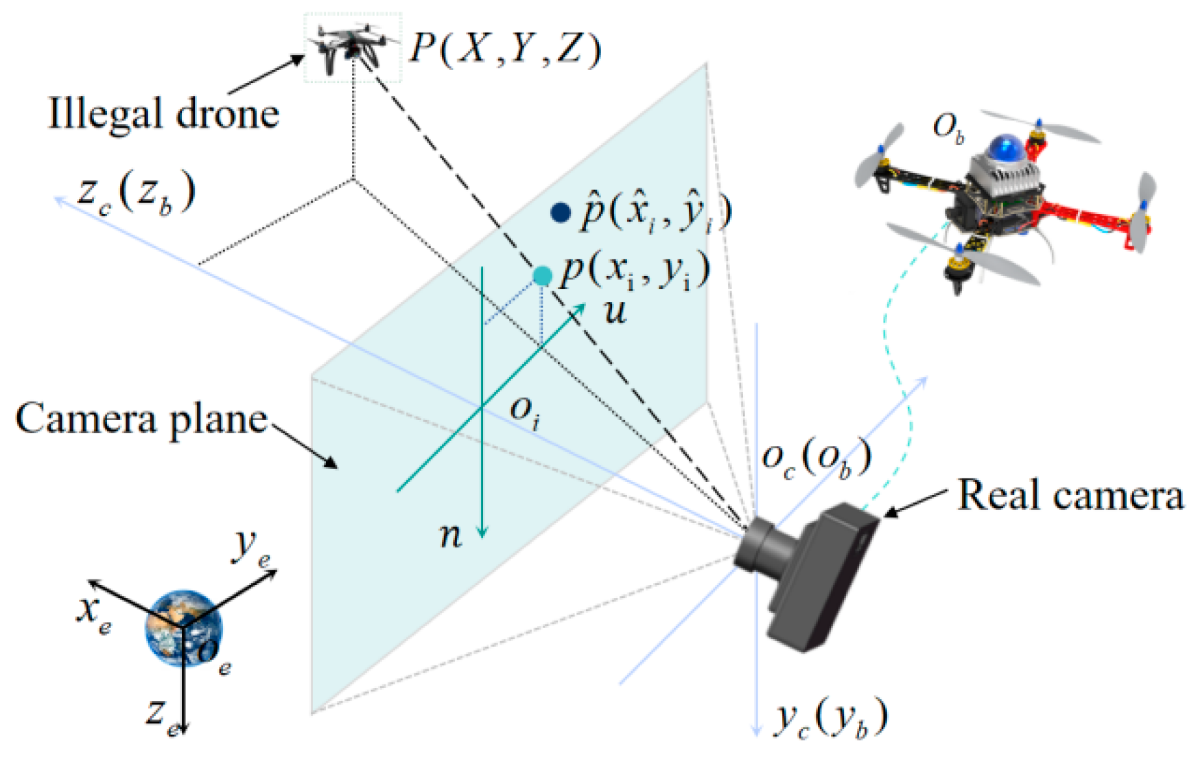
The core idea of IBVS is to achieve the coincidence of the future trajectory center coordinates of the illegal drone and the center coordinates of the manipulator claw in the pixel coordinate system {i} [35]. The relative positional relationships between the camera, camera plane, and the illegal drone are illustrated in Figure 3. In the figure, represents the camera coordinate system, and represents the pixel coordinate system.
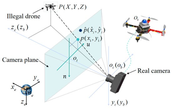
Figure 3.
Relative positional relationship between camera, camera plane and illegal drones.
The counter drone is equipped with a forward pinhole camera fixed on its lower part, denoted as coordinate system . and represent the image plane axis and the camera focal length, respectively. The quadcopter drone is an underactuated system. To decouple the dynamics of the quadcopter, a virtual camera frame is introduced. The origin of coincides with C, and the axis is always parallel to the axis. Additionally, the definition of the virtual image plane is similar to the definition of the image plane in C.
Assuming the illegal drone is a stationary target point P, with the world coordinate and the virtual camera frame, is and , respectively. Their transformation equations can be expressed as
where
Differentiating with respect to time
where the linear velocities of the illegal drone in the framesworld coordinate and virtual camera frame are denoted as and , respectively, with the unit vector .
Let the coordinates of the illegal drone P in the virtual image plane be labeled as P. The perspective projection equation in camera frame is then expressed as:
Substituting the above equation into Equation (11), the visual servoing equation is obtained, and the expression for the illegal drone P in the virtual image plane is:
where
Through the Jacobian matrix Jv in Equation (13), it is evident that is not related to the pitch and yaw angles of the counter drone. To maintain the stability of the counter drone’s flight, the desired pitch and yaw angles are set to zero.
Equation (13) expresses how the illegal drone moves in the image plane when the camera is in motion. For visual servoing, the focus is on its inverse problem—given the motion of the illegal drone in the camera plane, we determine the camera’s motion.
We then transform Equation (13) into:
The first term of corresponds to the velocity of the drone in the z-axis direction, denoted as B. Under the assumption of small perturbation linearization, the second term represents the angular rate of the desired roll angle. With this, the dynamic deconstruction of the counter drone in visual servoing is concluded.
2.3. Extended Kalman Filter Trajectory Prediction
To reach the interception position in advance, the EKF algorithm is employed to predict the position of the illegal drone in pixel coordinates. The EKF algorithm utilizes Taylor series expansion to linearize the treatment of nonlinear systems, followed by recursive computation and estimation. Its nonlinear expression is given by
In the equation, f(x) and h(x) represent the nonlinear mapping relationship; k is the time step; is the state vector; is the control vector; is the process noise; is the measurement vector; is the measurement noise; k−1 corresponds to the previous time step; ; ; ; ; is the observation error covariance matrix; is the measurement error covariance matrix.
The linearization process is as follows:
The linearized equation for Formula (11) is as follows:
The prediction process comprises a prediction equation and a correction equation.
Prediction Equation:
Correction Equation:
where ; represents the true value of the visual servoing feedback; is the a priori estimate; I is the identity matrix.
Directly predicting the coordinates in (x,y), we can define:
obtaining
We then define
and obtain
2.4. Controller Design
The goal of controller design is to endow the counter drone with high maneuverability and precision during the interception of the illegal drone, suppress disturbances caused by the illegal drone to the system, and achieve strong robustness.
Following the core idea of IBVS, the tracking error is defined as:
In the equation, and represent the tracking errors in the horizontal and vertical directions between the predicted center and the visual servoing center, respectively. denotes the coordinates of the visual servoing target point, chosen here as the center of the manipulator claw in the camera plane. represents the coordinates of the predicted center.
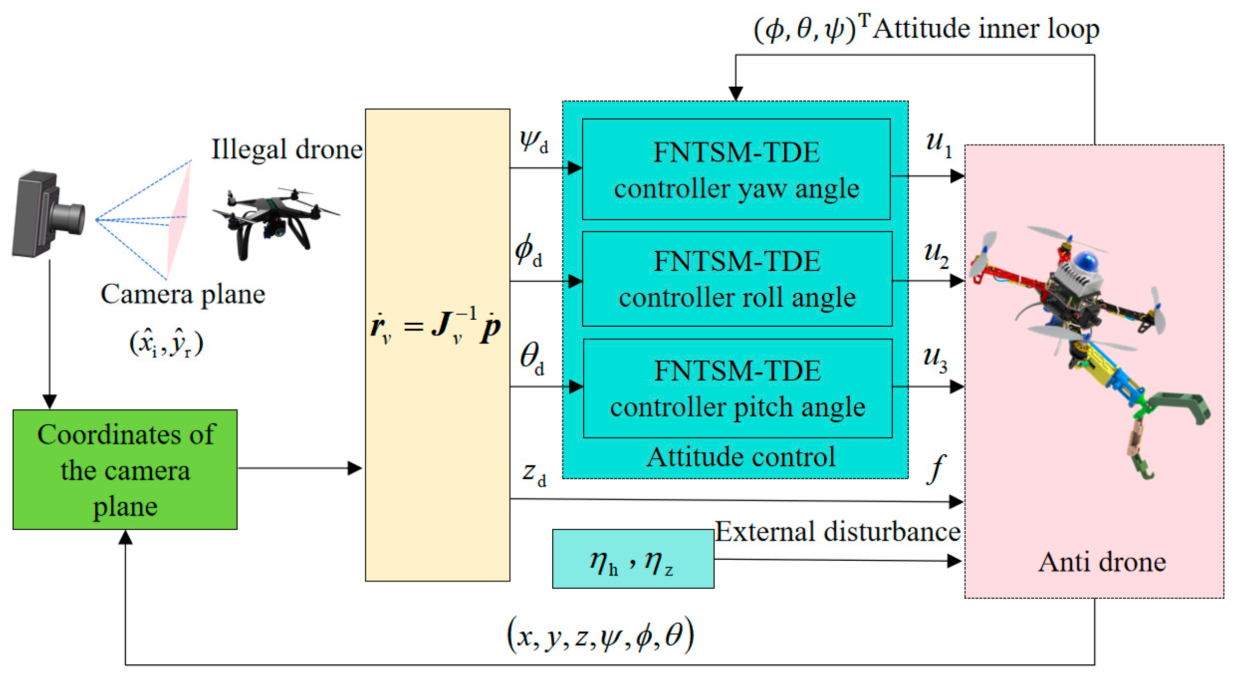
The drone’s control process is illustrated in Figure 4. To ensure the precise and rapid tracking of the target center in visual servoing, a controller is designed. We take the vertical channel as an example.

Figure 4.
Flight control structure diagram.
The following sliding mode surface [20] is chosen
where ; .
To eliminate oscillations and achieve finite-time convergence, the FTSM reaching law is employed.
where , is the sign function; ; .
The system’s stabilization time is
Since , considering Equation (4), the control law is designed as follows:
where .
Due to the inability to establish an accurate mathematical model for the impact disturbance at the moment of interception, the TDE technique is employed for online estimation and real-time compensation of unknown disturbances. This approach enables the acquisition of the nominal model of the controlled object, thereby simplifying the controller structure.
Based on the vertical channel’s dynamic model (4), in conjunction with Equation (27), the TDE technique is utilized to obtain :
where t represents the current time, and (t − k) corresponds to the current time delayed by k time. The complete expression of the control law is:
Similarly, the control law’s expression for the horizontal channel is
Taking the vertical channel as an example to demonstrate the stability of the proposed controller, the Lyapunov design is formulated as
The derivative with respect to time is
Taking the derivative of Equation (28) and substituting it into Equation (35), we get
By simultaneously solving Equations (30) and (31), we obtain
For the estimation error of TDE, there always exists a positive number such that is bounded, i.e., .
Substituting Equation (37) into Equation (36), we get:
The above equation is further discussed in the two cases
and
For equation (39), when , , the sliding surface can converge to the region in finite time
where .
For Equation (40), when , , the sliding surface can converge to the region in finite time
where .
Combining Equations (41) and (42), the sliding surface converges in finite time to
where .
3. Simulation and Experimentation
To validate the effectiveness of the proposed control strategy, Hardware in the Loop (HITL) [36] simulation experiments were conducted for algorithm verification. The HITL experiment involved the Robot Operating System (ROS) [37], Gazebo11 3D dynamic simulation software [38], and the Pixhawk 4 (PX 4) flight controller [39]. A repeatable, risk-free, and realistic simulation environment was established, incorporating physics characteristics such as collisions and aerodynamics to enhance development quality and efficiency. Subsequently, real flight experiments were conducted to optimize parameters during actual flights, further confirming the effectiveness of the proposed control strategy.
3.1. Hardware in the Loop Experiment
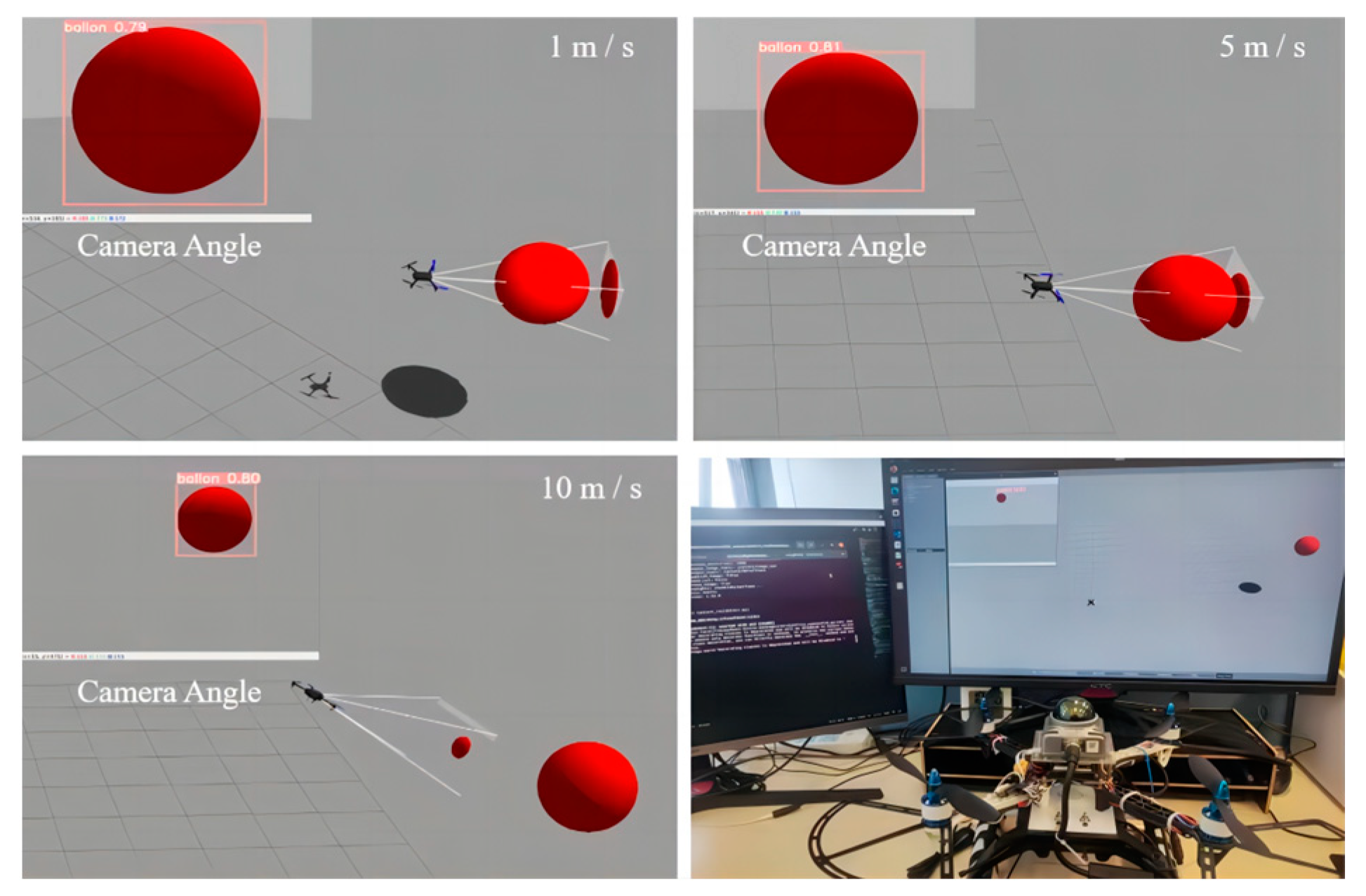
To simulate the states of actual flight, multiple states were set in the HITL simulation experiment, including environment initialization, take-off direction, target search, and tracking. Firstly, relevant scenes were created in the Gazebo 3D dynamic simulation environment, configured with capture objects, and simulated using an RGB camera to emulate a CCD industrial camera. Leveraging the distributed communication of the ROS system, target information was acquired, and the drone state was dynamically adjusted according to the proposed control strategy, reflecting real-time changes in the simulation scene. Finally, the PX 4 was used to control the drone to execute target capture tasks, as depicted in Figure 5 in the simulation scenario.

Figure 5.
HITL experiment.
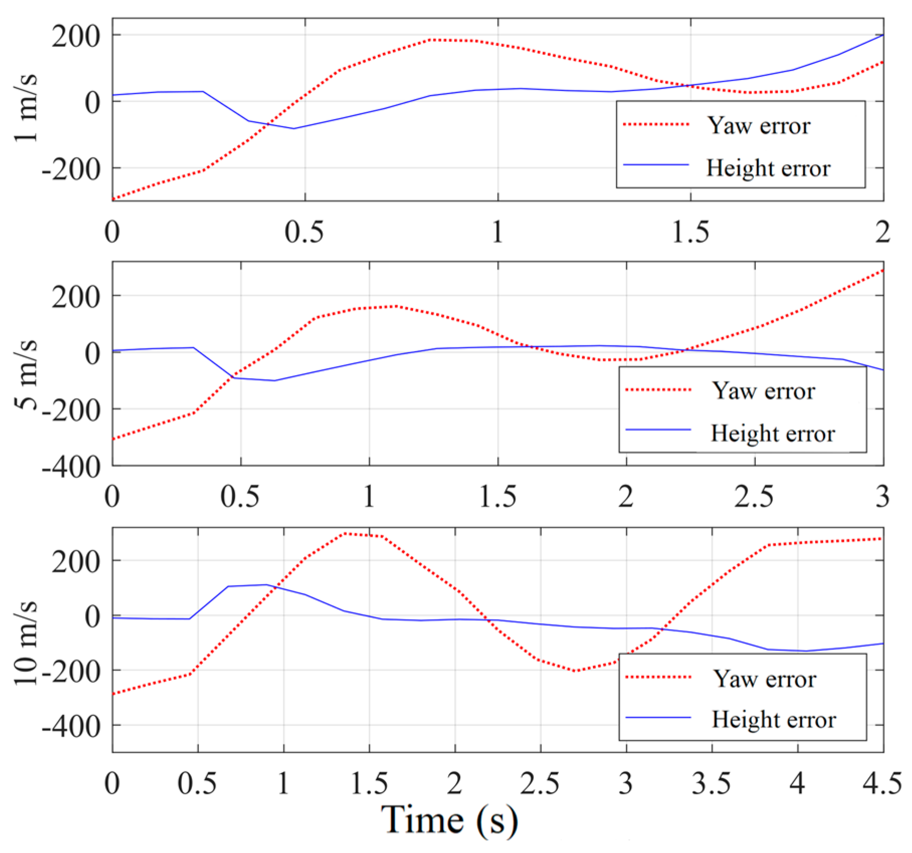
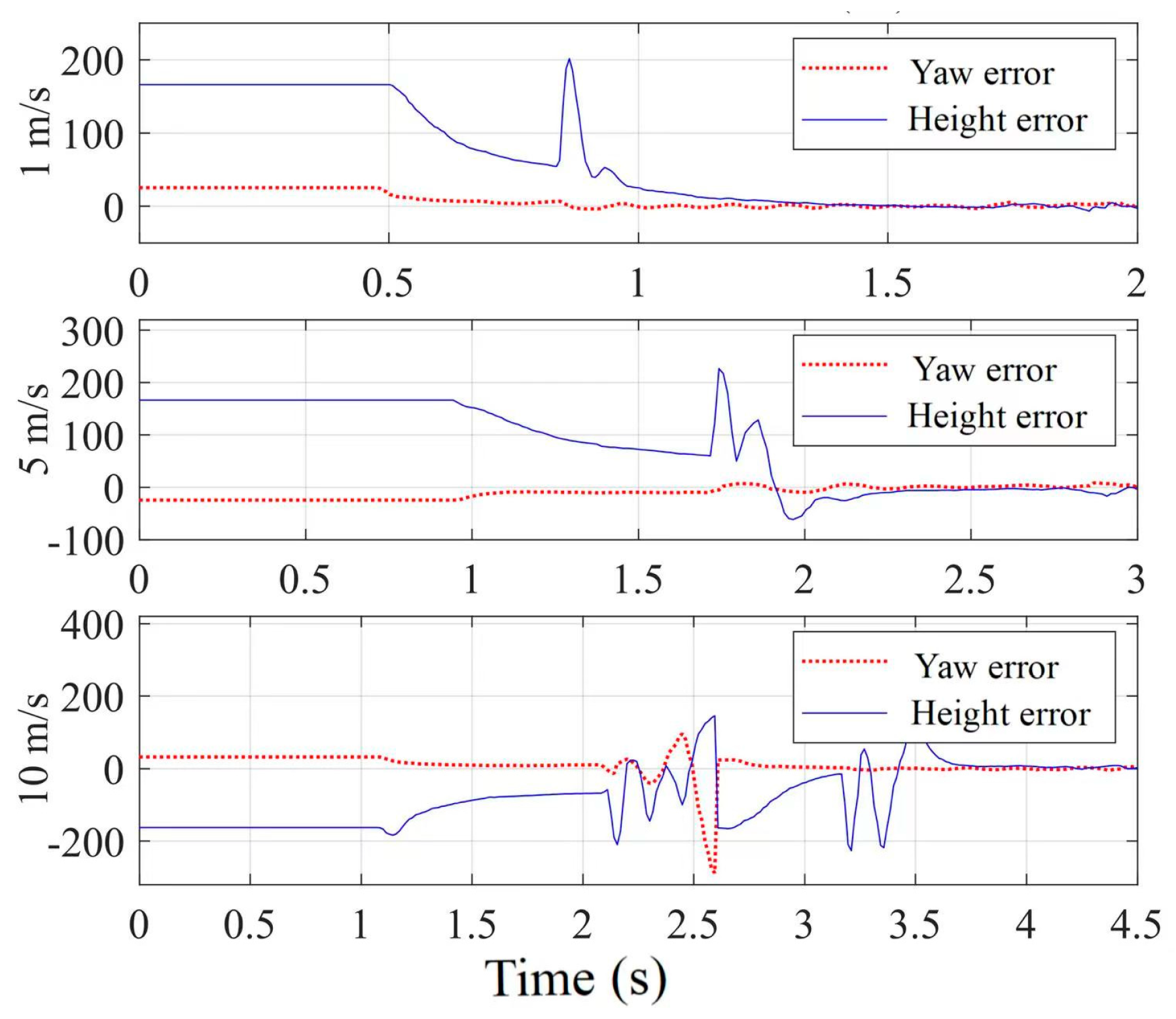
To reduce the requirements placed on the graphics card and enhance simulation efficiency, a red ball is used as a substitute for the illegal unmanned aerial vehicle. In the experiment, the red ball undergoes three-dimensional random movement with speeds set at 1 m/s, 5 m/s, and 10 m/s. The counter drone employs the same robust control strategy for tracking and capture. In the absence of EKF prediction, the tracking error in pixel coordinates is shown in Figure 6. When the tracking error is less than 20 pixels, it is considered as successfully tracking the target. In the HITL simulation experiments, the red ball moves at the aforementioned speeds, and the probabilities of the counter drone successfully tracking the target are 100%, 90%, and 12%, respectively. When EKF prediction is applied, the tracking error in pixel coordinates is shown in Figure 7, and the probabilities of the counter drone successfully tracking the target are 100%, 98%, and 80%, respectively. A comparison between Figure 6 and Figure 7 indicates that the use of EKF prediction improves the capture success rate and shortens the capture time. By predicting the future position of the target in advance, the drone can adjust its own state earlier for better target capture. When the red ball moves at a speed of 10 m/s, the counter drone approaches its thrust limit to catch up with the ball, and the pitch angle approaches 70° during acceleration. The HITL simulation results demonstrate that using EKF prediction allows for better target capture. As the target speed increases, both the drone’s flight speed and pitch angle show an increasing trend. Lower speeds result in a more stable capture process. The HITL simulation experiments also validate the robustness of the FNTSM-TDE control strategy.
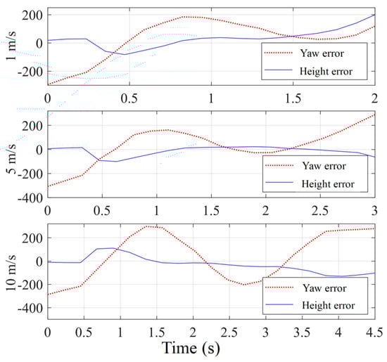
Figure 6.
Tracking error in the pixel coordinate system without EKF prediction in the simulation experiment.
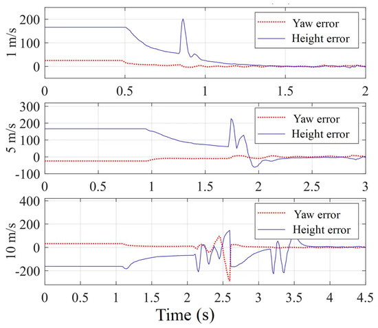
Figure 7.
Tracking error in the pixel coordinate system with EKF prediction in the simulation experiment.
Through HITL simulation experiments, the capture strategy is adjusted and optimized to more accurately capture the illegal unmanned aerial vehicle. In the visual servo system, controllers are designed by fully utilizing visual information, and the EKF algorithm is employed to predict the future trajectory of the illegal drone. Using the proposed controller as the underlying flight control strategy, the predicted trajectory is combined with the drone’s state, enabling the counter drone to obtain a feedforward control effect and enhance the capture success rate.
3.2. Flight Experiment
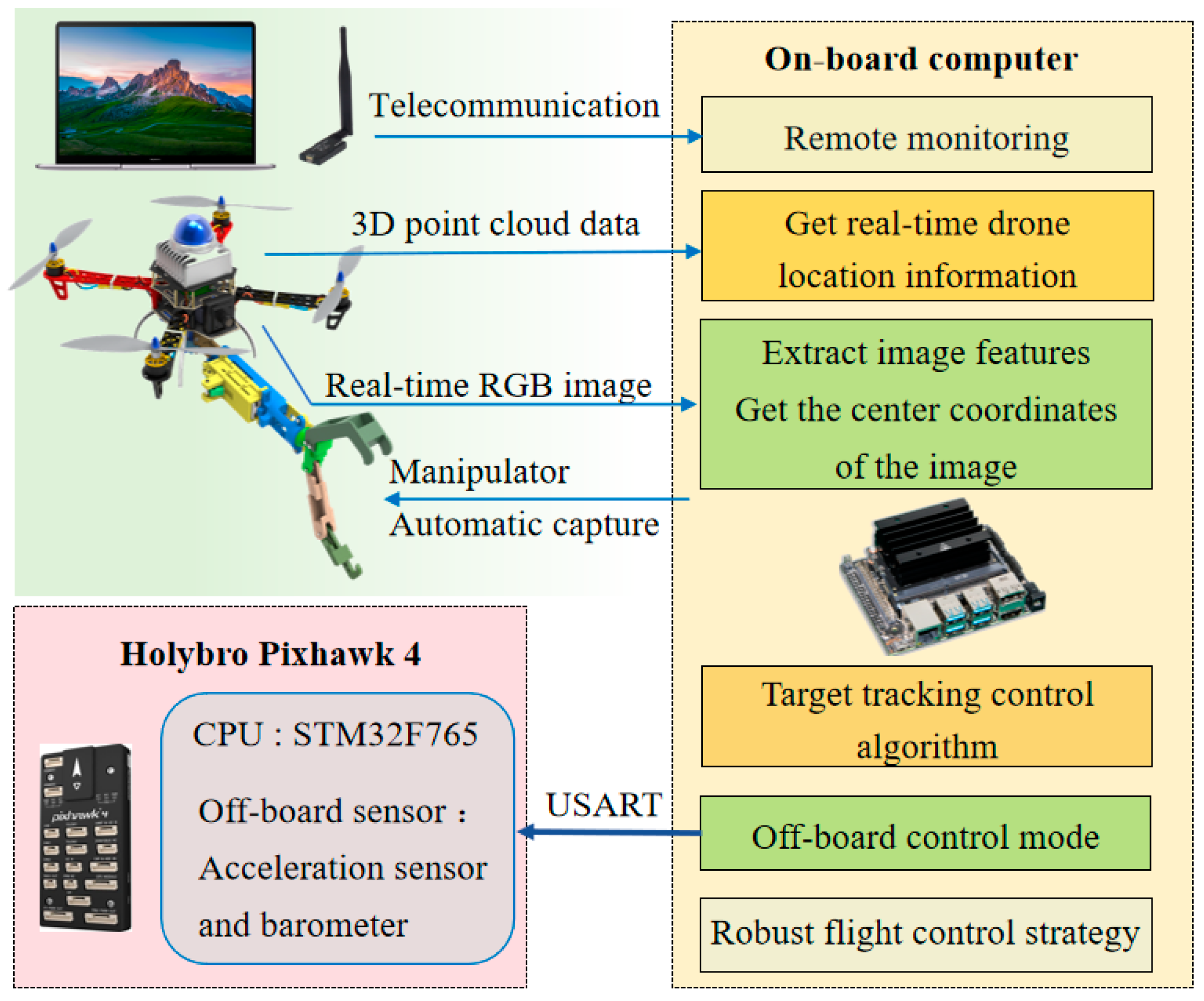
The counter drone comprises the drone mainframe and a manipulator suspended underneath. The top of the counter drone is equipped with the MID-360 laser radar, utilizing Simultaneous Localization and Mapping (SLAM) technology to create a high-resolution environmental map. By integrating SLAM technology and Inertial Measurement Unit (IMU) data, the counter drone obtains its own position, velocity, and acceleration. The system also includes an industrial camera and an on-board computer. The on-board computer is equipped with an Intel Core i7-1165G7 processor with 4 cores and 8 threads, used for running SLAM programs, recognizing the illegal drone, and running the EKF trajectory prediction program. The FNTSM-TDE control strategy operates within the PX 4, controlling the drone state and triggering manipulator actions.
The hardware composition schematic is shown in Figure 8. To meet the demands of rapid capture, the manipulator employs a passive triggering mechanism, utilizing elastic elements to store potential energy. When in contact with the illegal drone, the potential energy is converted into kinetic energy, causing the manipulator claws to close and capture the illegal drones. This design avoids the need for electronic devices such as sensors and drivers, and the weight of the manipulator is only 50 g, reducing the complexity and weight of the counter system.
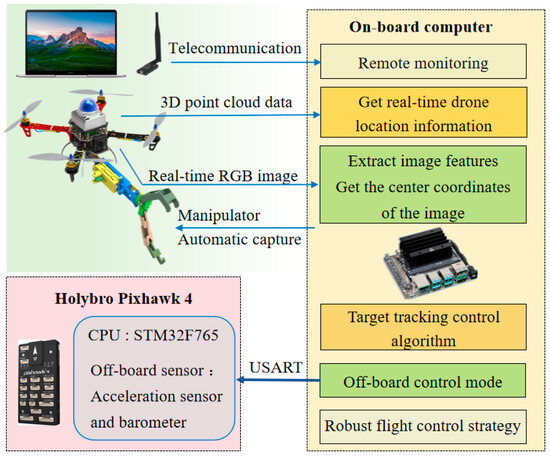
Figure 8.
Counter drone system hardware structure diagram.
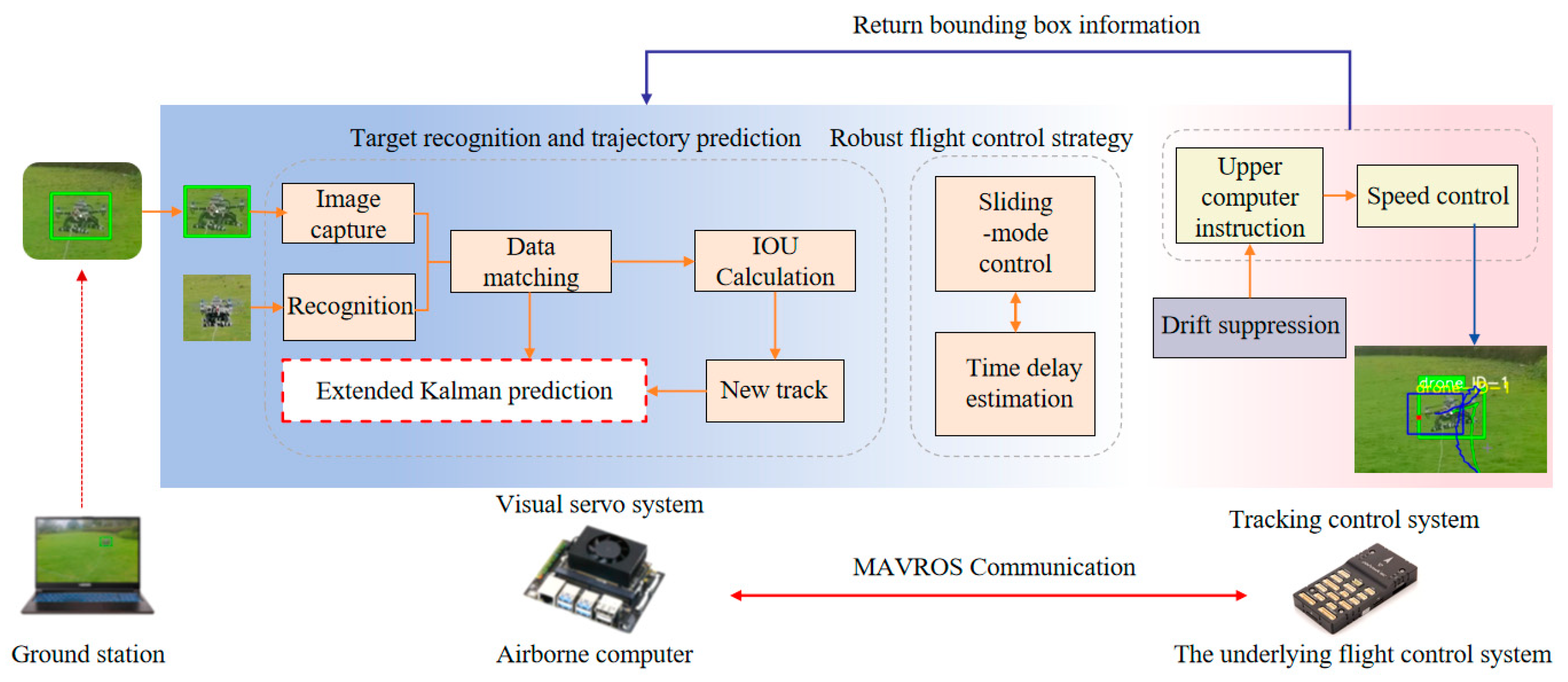
In the actual capture experiment, YOLOv5 technology was employed for target detection. To enhance tracking performance, a dataset comprising 6000 relevant drone images was collected and created. After 2500 iterations, the average Intersection over Union (IOU) on the test set reached 80%. To ensure accuracy and real-time capability, the video stream captured by the camera had a resolution of 1920 × 1080 pixels and a frame rate of 60 FPS. The overall system workflow is illustrated in Figure 9.
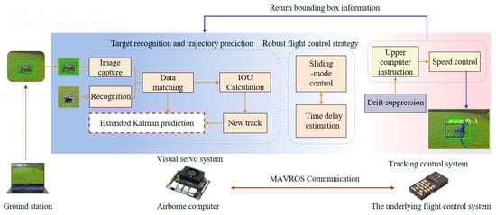
Figure 9.
Schematic diagram of the overall system structure.
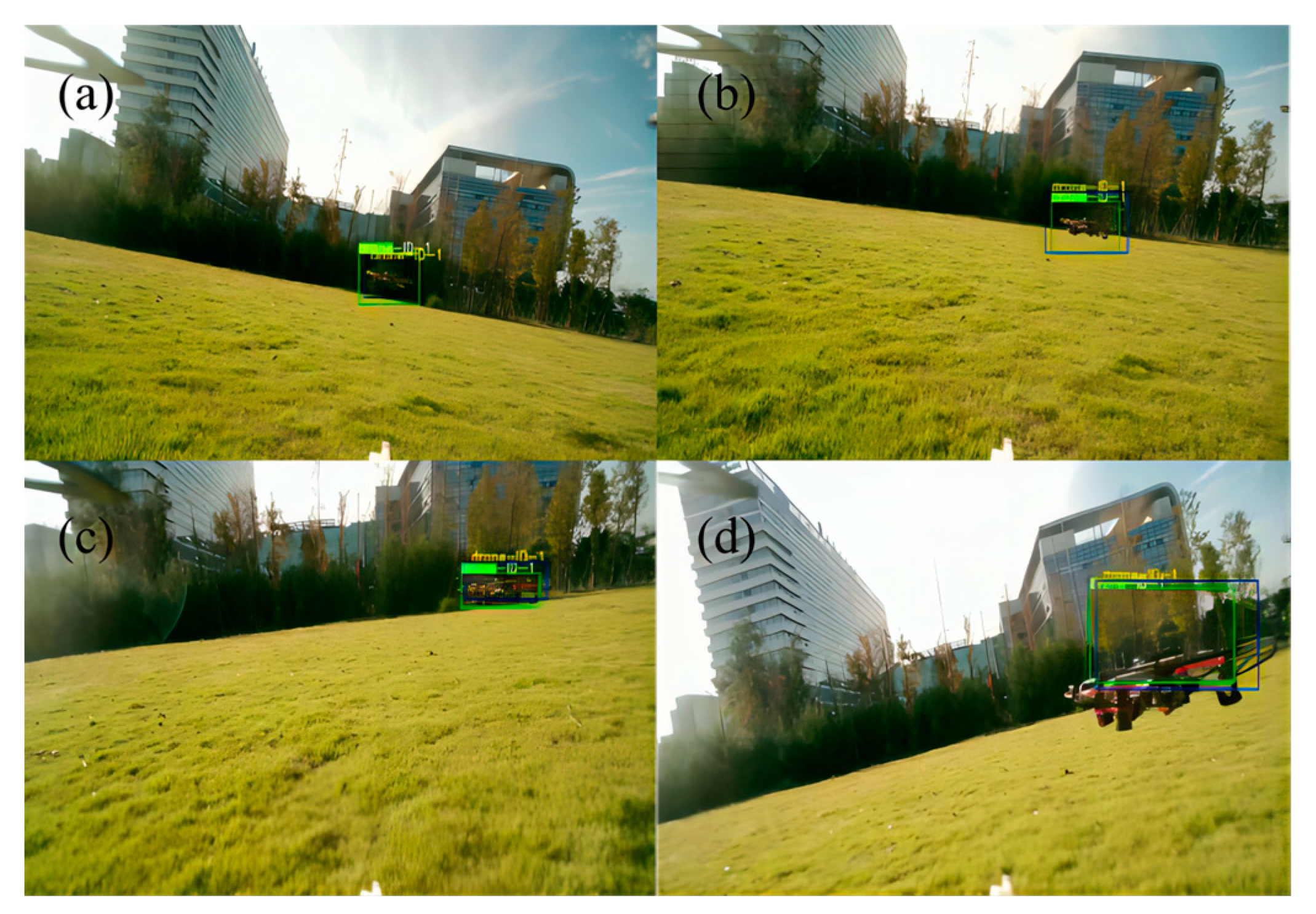
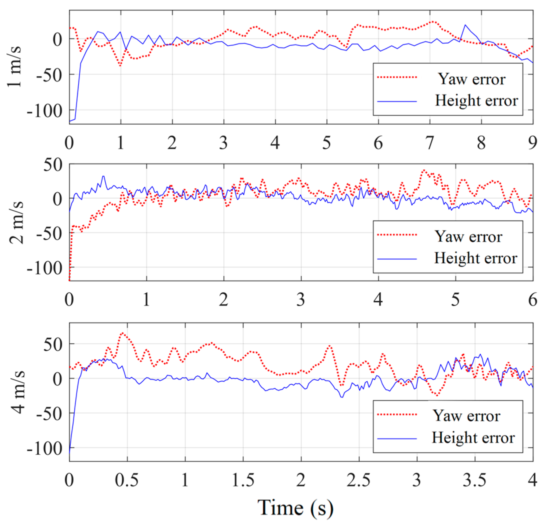
The flight experiment code is identical to the HITL, with the main difference lying in the source of sensor data. In the flight experiment, sensor signals come from the real world, whereas HITL receives sensor signals from the Gazebo 3D dynamic simulation software. In the experiment, the drone initially operates in the position mode, moving to a specified location. The counter drone possesses autonomous search capabilities, rotating around the Z-axis of its body to locate the target and bring the illegal drone into the camera’s field of view. Three capture experiments are conducted with the illegal drone flying at speeds of 1 m/s, 2 m/s, and 4 m/s, respectively. At the beginning of each experiment, the two drones are 8 m apart. Once the counter drone identifies the illegal drone, it autonomously predicts the future trajectory, adjusts its own state in real time, and tracks and captures the target. The capture process from the camera’s perspective is illustrated in Figure 10, where the YOLOv5 algorithm interprets the position of the illegal drone in the camera plane, and the EKF estimates its future trajectory. The four sub images represent the images and recognition effects captured by the drone at different positions and attitude angles, respectively. The pixel error curve during the capture process is shown in Figure 11. Due to the EKF algorithm predicting the trajectory of the illegal drone in advance, the tracking error rapidly converges to zero. In experiments without the EKF algorithm, the convergence time of the tracking error increased by a factor of 2.
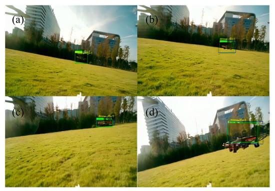
Figure 10.
(a–d) The capture process from the camera’s perspective at different positions and attitude angles, respectively.
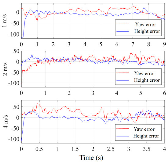
Figure 11.
Tracking error in the pixel coordinate system in real time.
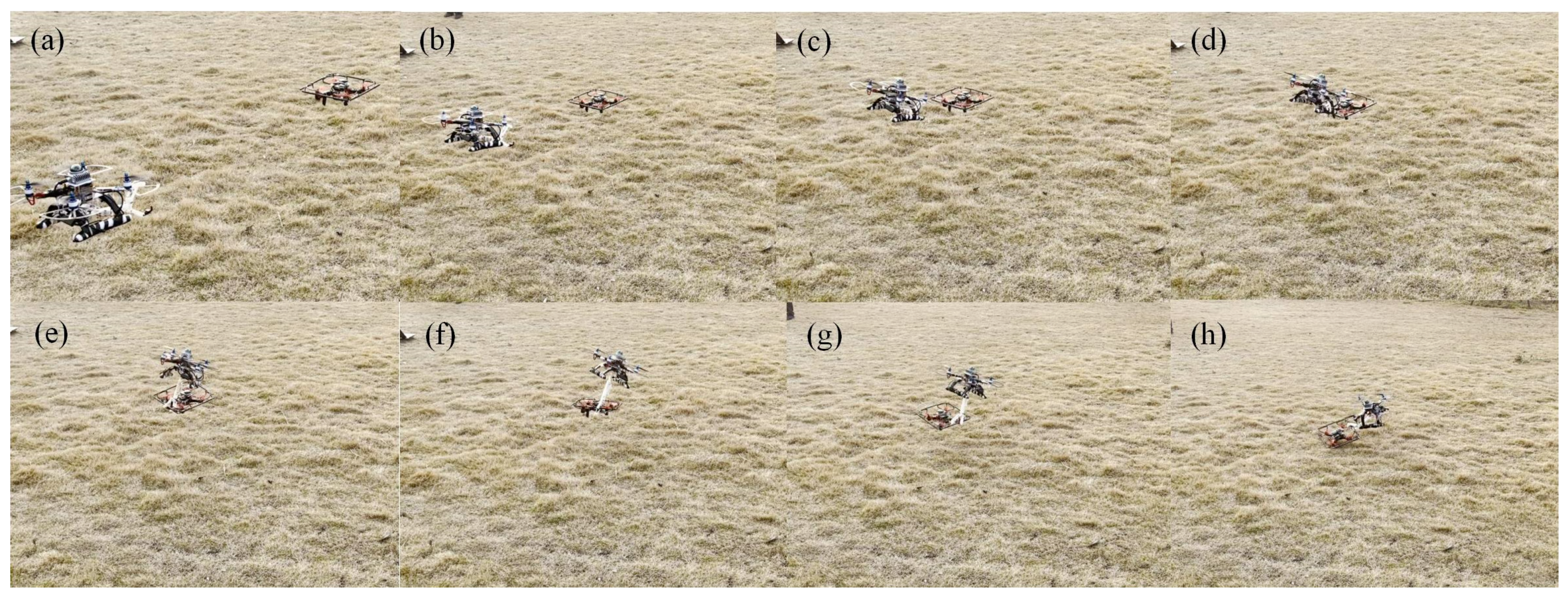
The eight subplots in Figure 12 depict capture scenes of the counter drone, demonstrating its autonomous tracking of the illegal drone and the automatic triggering and capture of the illegal drone by the manipulator. Once the manipulator makes contact with the illegal drone, the elastic elements are automatically triggered, and the claws of the manipulator capture the illegal drone.
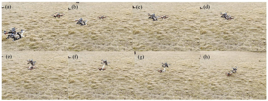
Figure 12.
(a–h) Eight capture scenes of the counter drone capturing an illegal drone.
4. Conclusions
This paper presents an airspace management strategy based on IBVS, utilizing a counter drone equipped with a robotic arm to capture illegal drones. The strategy achieves triple functionality: utilizing a neural network model based on the YOLO-v5 architecture for the visual recognition of an illegal drone, employing EKF for the advanced prediction of illegal drone flight trajectories to enhance capture success rates, utilizing a lightweight passive trigger mechanical hand weighing only 50 g for drone capture to reduce the weight and complexity of the capture system, and proposing the FNTSM-TDE control strategy to suppress the interference of rogue drones with counter UAVs during capture moments. This strategy features advantages of model-free control and finite-time convergence. The effectiveness of the proposed control strategy is validated through HITL simulation experiments and real flight tests. The EKF algorithm is employed to predict rogue drone trajectories in advance, resulting in the accelerated convergence of tracking errors to zero. Compared to capture strategies without EKF configuration, the convergence time is halved, thus enhancing capture success rates. Future efforts will focus on conducting capture experiments in more diverse scenarios to further enhance the robustness and practicality of the system.
5. Patents
The key technology disclosed in the paper has been applied for an invention patent in China, named an unpowered adaptive fast linkage manipulator and a drone capture device, patent No. 202311365289.2.
Author Contributions
Conceptualization and funding acquisition S.Y. and P.C.; methodology, validation, and data curation J.M.; visualization D.Z.; software, investigation, and formal analysis X.X. and L.Z. All authors have read and agreed to the published version of the manuscript.
Funding
This research was funded by the Wenzhou Key Laboratory of Biomaterials and Engineering, Wenzhou Institute, University of Chinese Academy of Sciences under Grant No. WIUCASSWCL21002, Wenzhou Scientific Research Project under Grant No. G20210045, Wenzhou Research Institute of the University of Chinese Academy of Sciences under Grant No. WIUCASQD2021009, Wenzhou Key Scientific Research Project under Grant No. ZGF2023056. The authors gratefully acknowledge the assistance of these support agencies.
Data Availability Statement
The data that support the findings of this study are available from the corresponding author upon reasonable request.
Conflicts of Interest
Author Xinhan Xiong and Liangcheng Zhang were employed by the company Zhejiang Gold Intelligent Suspension Corp, author Dongyuan Zhang was employed by the company Beiing CRRC CED Railway Electrical Technology Company. The remaining authors declare that the research was conducted in the absence of any commercial or financial relationships that could be construed as a potential conflict of interest.
References
- Pounds, P.E.I.; Deer, W. The safety rotor—An electromechanical rotor safety system for drones. IEEE Robot. Autom. Lett. 2018, 3, 2561–2568. [Google Scholar] [CrossRef]
- Ayamga, M.; Akaba, S.; Nyaaba, A.A. Multifaceted applicability of drones: A review. Technol. Forecast. Soc. Change 2021, 167, 120677. [Google Scholar] [CrossRef]
- Lee, I.J.; Choi, S.H.; Joo, I.O.; Jeon, J.W.; Cha, J.H.; Ahn, J.Y. Technical Trends on Low-Altitude Drone Detection Technology for Countering Illegal Drones. Electron. Telecommun. Trends 2022, 37, 10–20. [Google Scholar]
- Calcara, A.; Gilli, A.; Gilli, M.; Marchetti, R.; Zaccagnini, I. Why drones have not revolutionized war: The enduring hider-finder competition in air warfare. Int. Secur. 2022, 46, 130–171. [Google Scholar] [CrossRef]
- Hussain, A.; Saqib, N.A.; Qamar, U.; Zia, M.; Mahmood, H. Protocol-aware radio frequency jamming in Wi-Fi and commercial wireless networks. J. Commun. Netw. 2014, 16, 397–406. [Google Scholar] [CrossRef]
- Krayani, A.; Alam, A.S.; Marcenaro, L.; Nallanathan, A.; Regazzoni, C. Automatic Jamming Signal Classification in Cognitive UAV Radios. IEEE Trans. Veh. Technol. 2022, 71, 12972–12988. [Google Scholar] [CrossRef]
- Wang, J.; Jiang, C.; Kuang, L. High-mobility satellite-UAV communications: Challenges, solutions, and future research trends. IEEE Commun. Mag. 2022, 60, 38–43. [Google Scholar] [CrossRef]
- Wang, T.; Chen, B.; Zhang, Z.; Li, H.; Zhang, M. Applications of machine vision in agricultural robot navigation: A review. Comput. Electron. Agric. 2022, 198, 107085. [Google Scholar] [CrossRef]
- Lien, J.; Gillian, N.; Karagozler, M.E.; Amihood, P.; Schwesig, C.; Olson, E.; Raja, H.; Poupyrev, I. Soli: Ubiquitous gesture sensing with millimeter wave radar. ACM Trans. Graph. (TOG) 2016, 35, 1–19. [Google Scholar] [CrossRef]
- Wallace, L.; Lucieer, A.; Watson, C.S. Evaluating tree detection and segmentation routines on very high resolution UAV LiDAR data. IEEE Trans. Geosci. Remote Sens. 2014, 52, 7619–7628. [Google Scholar] [CrossRef]
- Jiang, P.; Ergu, D.; Liu, F.; Cai, Y.; Ma, B. A Review of Yolo algorithm developments. Procedia Comput. Sci. 2022, 199, 1066–1073. [Google Scholar] [CrossRef]
- Zhu, W.; Zhang, H.; Eastwood, J.; Qi, X.; Jia, J.; Cao, Y. Concrete crack detection using lightweight attention feature fusion single shot multibox detector. Knowl. Based Syst. 2023, 261, 110216. [Google Scholar] [CrossRef]
- Sankareshwaran, S.P.; Jayaraman, G.; Muthukumar, P.; Krishnan, A. Optimizing rice plant disease detection with crossover boosted artificial hummingbird algorithm based AX-RetinaNet. Environ. Monit. Assess. 2023, 195, 1070. [Google Scholar] [CrossRef] [PubMed]
- Vijayakumar, V.; Ampatzidis, Y.; Costa, L. Tree-level citrus yield prediction utilizing ground and aerial machine vision and machine learning. Smart Agric. Technol. 2023, 3, 100077. [Google Scholar] [CrossRef]
- Wu, J.; Jin, Z.; Liu, A.; Yu, L.; Yang, F. A survey of learning-based control of robotic visual servoing systems. J. Frankl. Inst. 2022, 359, 556–577. [Google Scholar] [CrossRef]
- Li, Z.; Lai, B.; Pan, Y. Image-based composite learning robot visual servoing with an uncalibrated eye-to-hand camera. IEEE/ASME Trans. Mechatron. 2024. [Google Scholar] [CrossRef]
- Costanzo, M.; De Maria, G.; Natale, C.; Russo, A. Modeling and Control of Sampled-Data Image-Based Visual Servoing with Three-Dimensional Features. IEEE Trans. Control Syst. Technol. 2023, 32, 31–46. [Google Scholar] [CrossRef]
- Ribeiro, E.G.; Mendes, R.Q.; Terra, M.H.; Grassi, V. Second-Order Position-Based Visual Servoing of a Robot Manipulator. IEEE Robot. Autom. Lett. 2023, 9, 207–214. [Google Scholar] [CrossRef]
- Miranda-Moya, A.; Castañeda, H.; Gordillo, J.L.; Wang, H. Ibvs based on adaptive sliding mode control for a quadrotor target tracking under perturbations. Mechatronics 2022, 88, 102909. [Google Scholar] [CrossRef]
- Li, B.; Na, Z.; Lin, B. Uav trajectory planning from a comprehensive energy efficiency perspective in harsh environments. IEEE Netw. 2022, 36, 62–68. [Google Scholar] [CrossRef]
- Zhang, J.D.; Shi, Z.Y.; Zhang, A.L.; Yang, Q.M.; Shi, G.Q.; Wu, Y. UAV Trajectory Prediction Based on Flight State Recognition. IEEE Trans. Aerosp. Electron. Syst. 2023. [Google Scholar] [CrossRef]
- Ostrowski, M.; Blachowski, B.; Mikułowski, G.; Jankowski, Ł. Influence of Noise in Computer-Vision-Based Measurements on Parameter Identification in Structural Dynamics. Sensors 2022, 23, 291. [Google Scholar] [CrossRef] [PubMed]
- Hossain, M.; Haque, M.E.; Arif, M.T. Kalman filtering techniques for the online model parameters and state of charge estimation of the Li-ion batteries: A comparative analysis. J. Energy Storage 2022, 51, 104174. [Google Scholar] [CrossRef]
- Singh, H.; Chattopadhyay, A.; Mishra, K.V. Inverse Extended Kalman Filter—Part I: Fundamentals. IEEE Trans. Signal Process. 2023, 71, 2936–2951. [Google Scholar] [CrossRef]
- Yu, S.; Xie, M.; Ma, J.; Yao, J.; Pan, L.; Wu, H. Precise robust motion tracking of a piezoactuated micropuncture mechanism with sliding mode control. J. Frankl. Inst. 2021, 358, 4410–4434. [Google Scholar] [CrossRef]
- Brahmi, B.; Driscoll, M.; El Bojairami, I.K.; Saad, M.; Brahmi, A. Novel adaptive impedance control for exoskeleton robot for rehabilitation using a nonlinear time-delay disturbance observer. ISA Trans. 2021, 108, 381–392. [Google Scholar] [CrossRef]
- Yu, S.; Wu, H.; Xie, M.; Lin, H.; Ma, J. Precise robust motion control of cell puncture mechanism driven by piezoelectric actuators with fractional-order nonsingular terminal sliding mode control. Bio-Des. Manuf. 2020, 3, 410–426. [Google Scholar] [CrossRef]
- Gambhire, S.J.; Kishore, D.R.; Londhe, P.S.; Pawar, S. Review of sliding mode based control techniques for control system applications. Int. J. Dyn. Control 2021, 9, 363–378. [Google Scholar] [CrossRef]
- Yu, S.; Xie, M.; Wu, H.; Ma, J.; Li, Y.; Gu, H. Composite proportional-integral sliding mode control with feedforward control for cell puncture mechanism with piezoelectric actuation. ISA Trans. 2022, 124, 427–435. [Google Scholar] [CrossRef]
- Ma, J.; Xie, M.; Chen, P.; Yu, S.; Zhou, H. Motion tracking of a piezo-driven cell puncture mechanism using enhanced sliding mode control with neural network. Control Eng. Pract. 2023, 134, 105487. [Google Scholar] [CrossRef]
- Xie, M.; Yu, S.; Lin, H.; Ma, J.; Wu, H. Improved sliding mode control with time delay estimation for motion tracking of cell puncture mechanism. IEEE Trans. Circuits Syst. I: Regul. Pap. 2020, 67, 3199–3210. [Google Scholar] [CrossRef]
- Wang, X.; van Kampen, E.-J.; Chu, Q. Quadrotor fault-tolerant incremental nonsingular terminal sliding mode control. Aerosp. Sci. Technol. 2019, 95, 105514. [Google Scholar] [CrossRef]
- Labbadi, M.; Cherkaoui, M. Novel robust super twisting integral sliding mode controller for a quadrotor under external disturbances. Int. J. Dyn. Control 2020, 8, 805–815. [Google Scholar] [CrossRef]
- Qiu, Z.; Bai, H.; Chen, T. Special Vehicle Detection from UAV Perspective via YOLO-GNS Based Deep Learning Network. Drones 2023, 7, 11. [Google Scholar] [CrossRef]
- Cintas, E.; Ozyer, B.; Simsek, E. Vision-based moving UAV tracking by another UAV on low-cost hardware and a new ground control station. IEEE Access 2020, 8, 194601–194611. [Google Scholar] [CrossRef]
- Haase, P.; Thomas, B. Test and optimization of a control algorithm for demand-oriented operation of CHP units using hardware-in-the-loop. Appl. Energy 2021, 294, 116974. [Google Scholar] [CrossRef]
- Macenski, S.; Foote, T.; Gerkey, B.; Lalancette, C.; Woodall, W. Robot Operating System 2: Design, architecture, and uses in the wild. Sci. Robot. 2022, 7, eabm6074. [Google Scholar] [CrossRef] [PubMed]
- Platt, J.; Ricks, K. Comparative Analysis of ROS-Unity3D and ROS-Gazebo for Mobile Ground Robot Simulation. J. Intell. Robot. Syst. 2022, 106, 80. [Google Scholar] [CrossRef]
- Nguyen, K.D.; Ha, C. Development of hardware-in-the-loop simulation based on gazebo and pixhawk for unmanned aerial vehicles. Int. J. Aeronaut. Space Sci. 2018, 19, 238–249. [Google Scholar] [CrossRef]

Disclaimer/Publisher’s Note: The statements, opinions and data contained in all publications are solely those of the individual author(s) and contributor(s) and not of MDPI and/or the editor(s). MDPI and/or the editor(s) disclaim responsibility for any injury to people or property resulting from any ideas, methods, instructions or products referred to in the content. |
© 2024 by the authors. Licensee MDPI, Basel, Switzerland. This article is an open access article distributed under the terms and conditions of the Creative Commons Attribution (CC BY) license (https://creativecommons.org/licenses/by/4.0/).