
LAEA: A 2D LiDAR-Assisted UAV Exploration Algorithm for Unknown Environments


Abstract
1. Introduction
- (1)
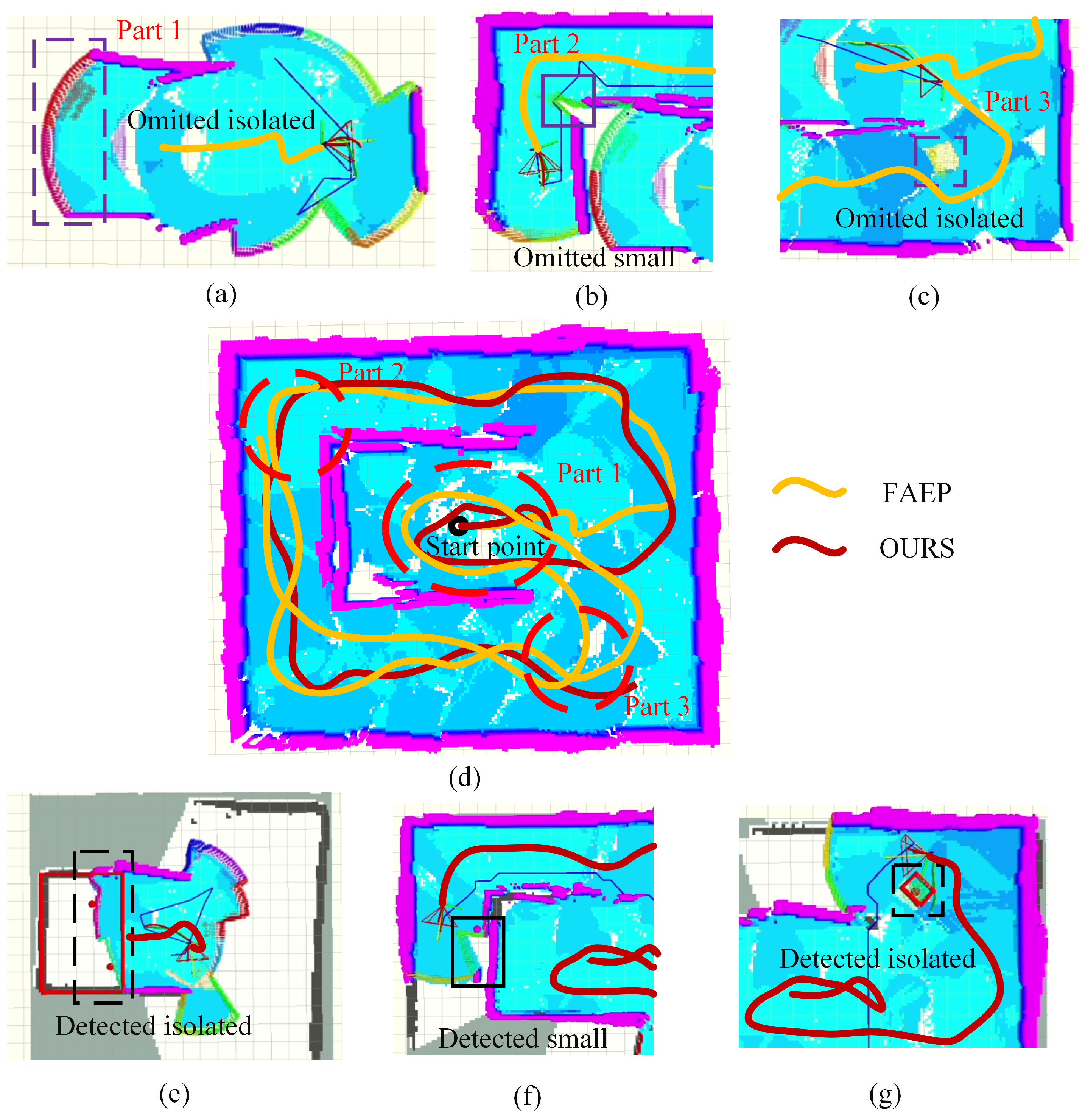
- The improper characterization of small frontier clusters leads the UAV to neglect such areas, which results in back-and-forth movements;
- (2)
- Frontiers adjacent to the flight trajectories to targets are often overlooked, which could also lead to back-and-forth movements.
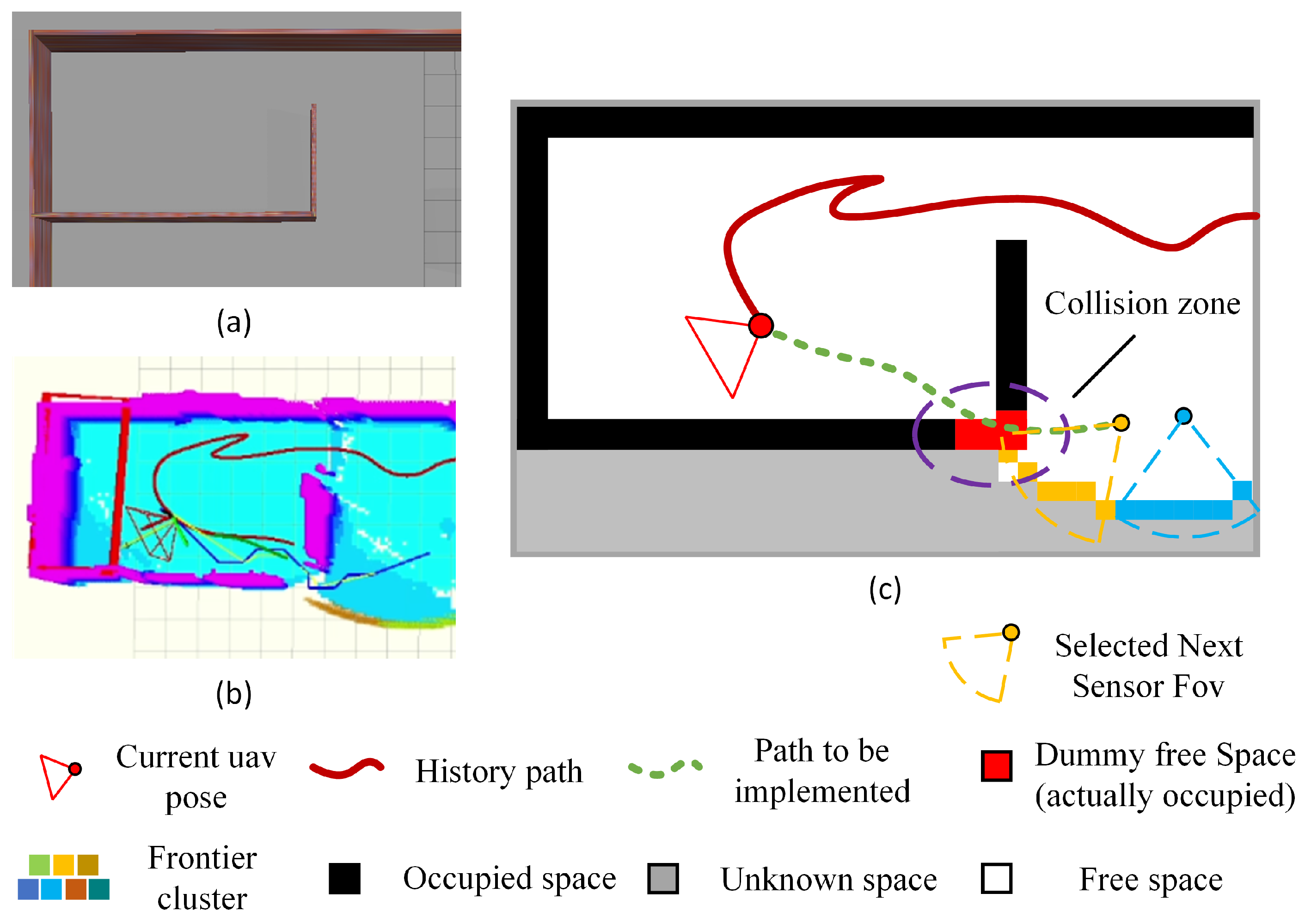
- A hybrid 2D map is constructed that offers a more effective method to detect and prioritize visits to small and isolated frontier clusters, which could reduce back-and-forth movements.
- An EIG optimization strategy is proposed that significantly improves the coverage of unknown frontier clusters during the UAV’s flight to the next target, as well as flight safety.
- The proposed algorithm is compared with two state-of-the-art algorithms through simulation, and then, validated on a robotic platform in different real-world scenarios.
2. Related Works
2.1. Sampling-Based Methods
2.2. Frontier-Based Methods
3. Proposed Method
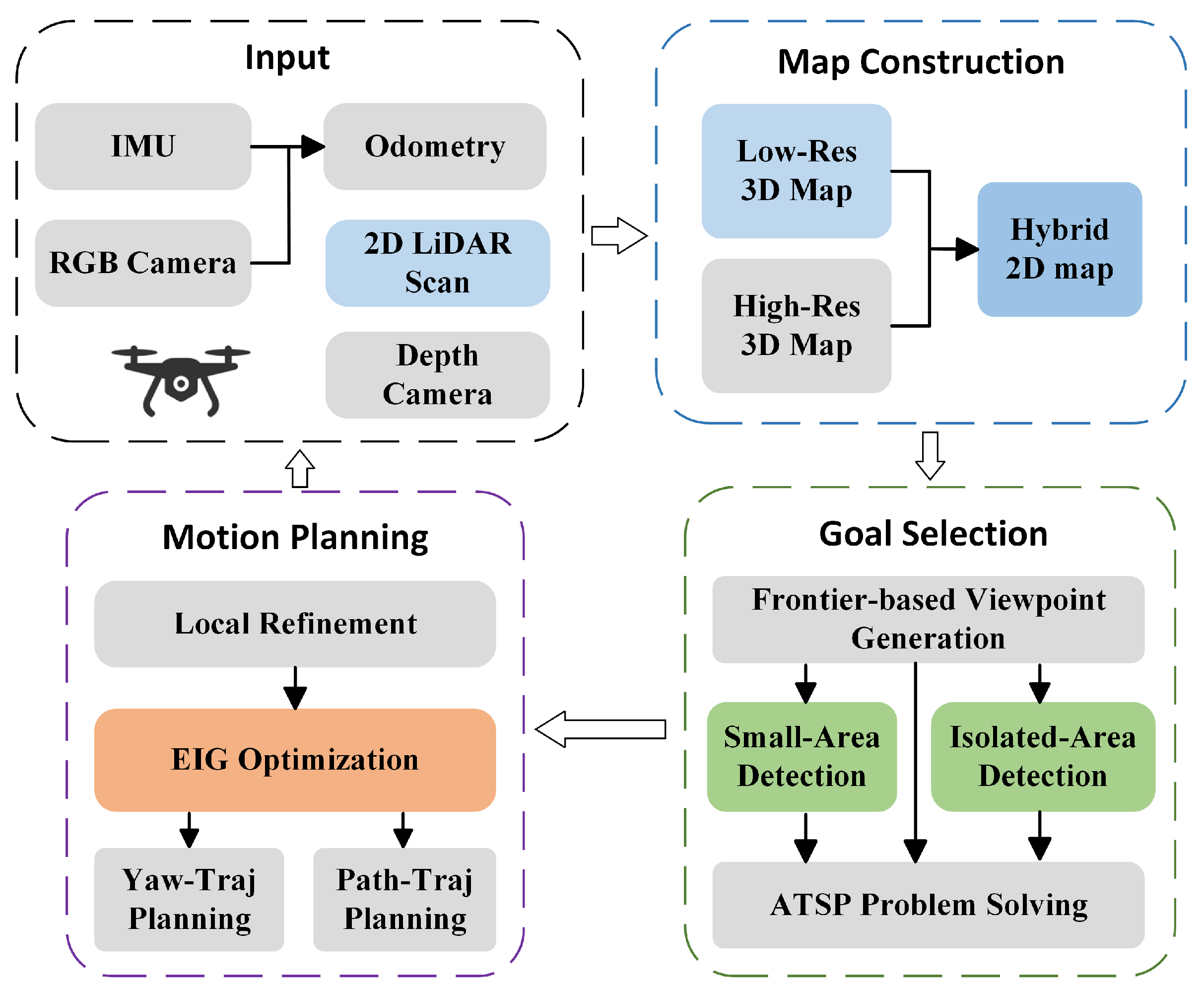
3.1. System Overview
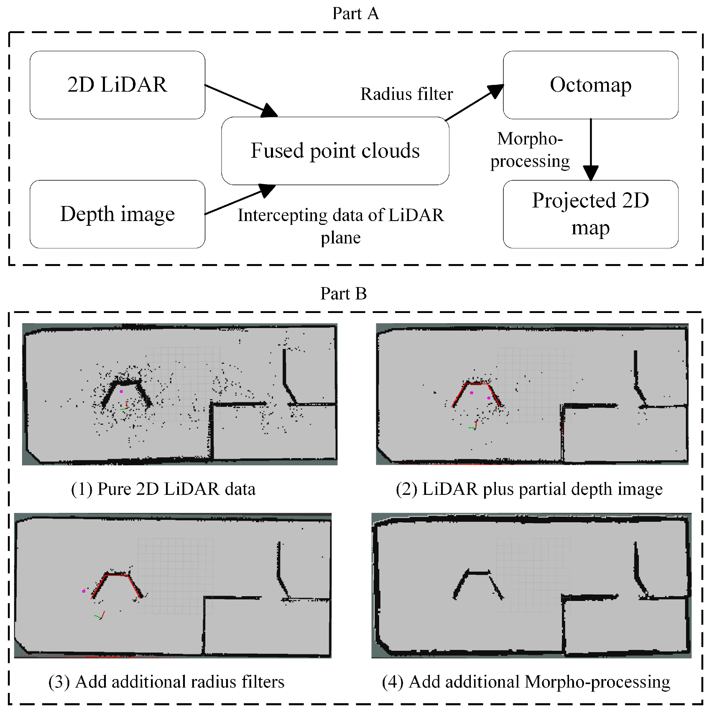
3.2. Map Construction Module
3.3. Target Selection Module
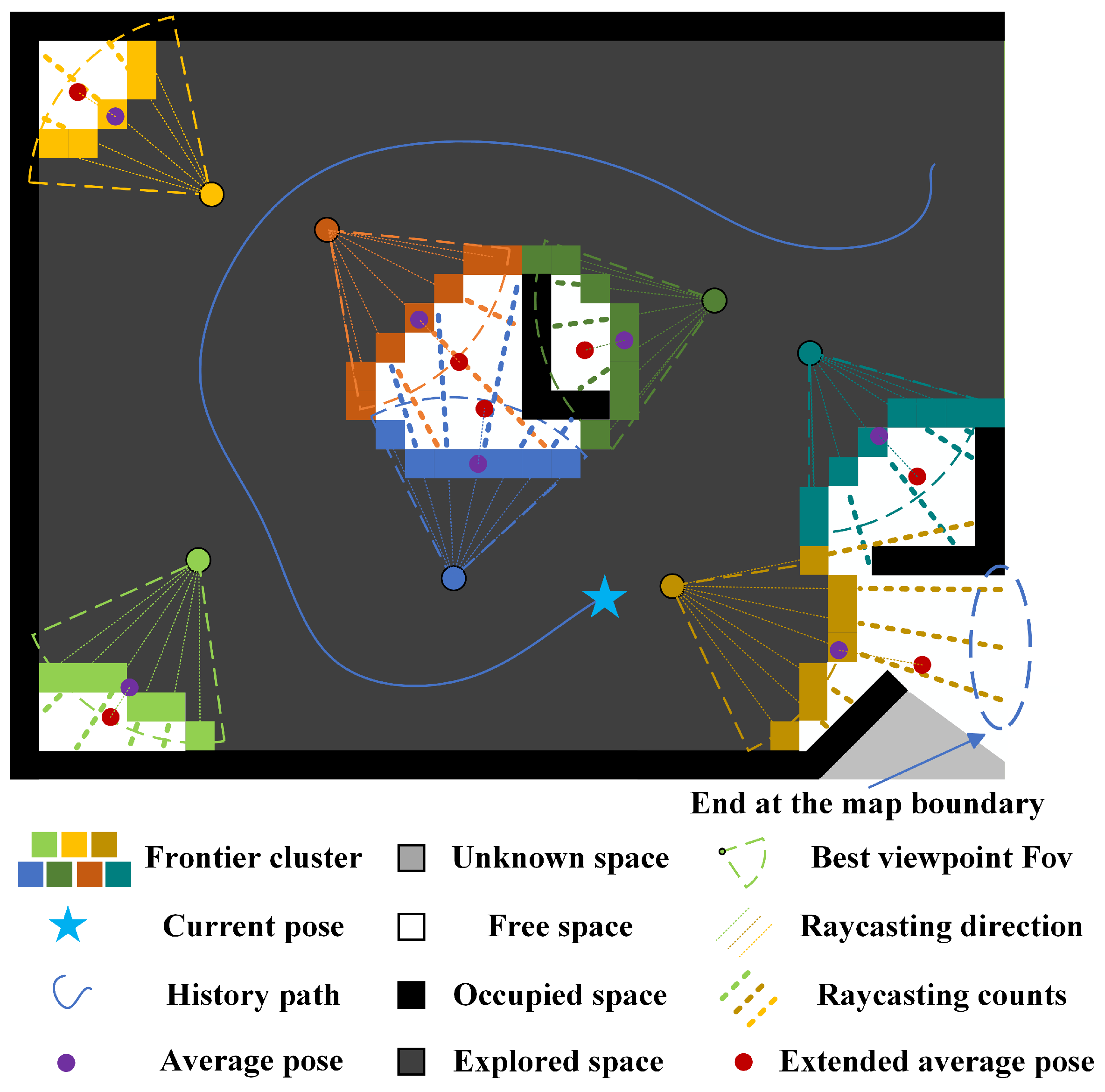
3.3.1. Frontier-Based Viewpoint Generation
3.3.2. Small-Area Cluster Detection
| Algorithm 1 Calculation of LiDAR information gain. |
| Input: , , , , Output: , ,
|
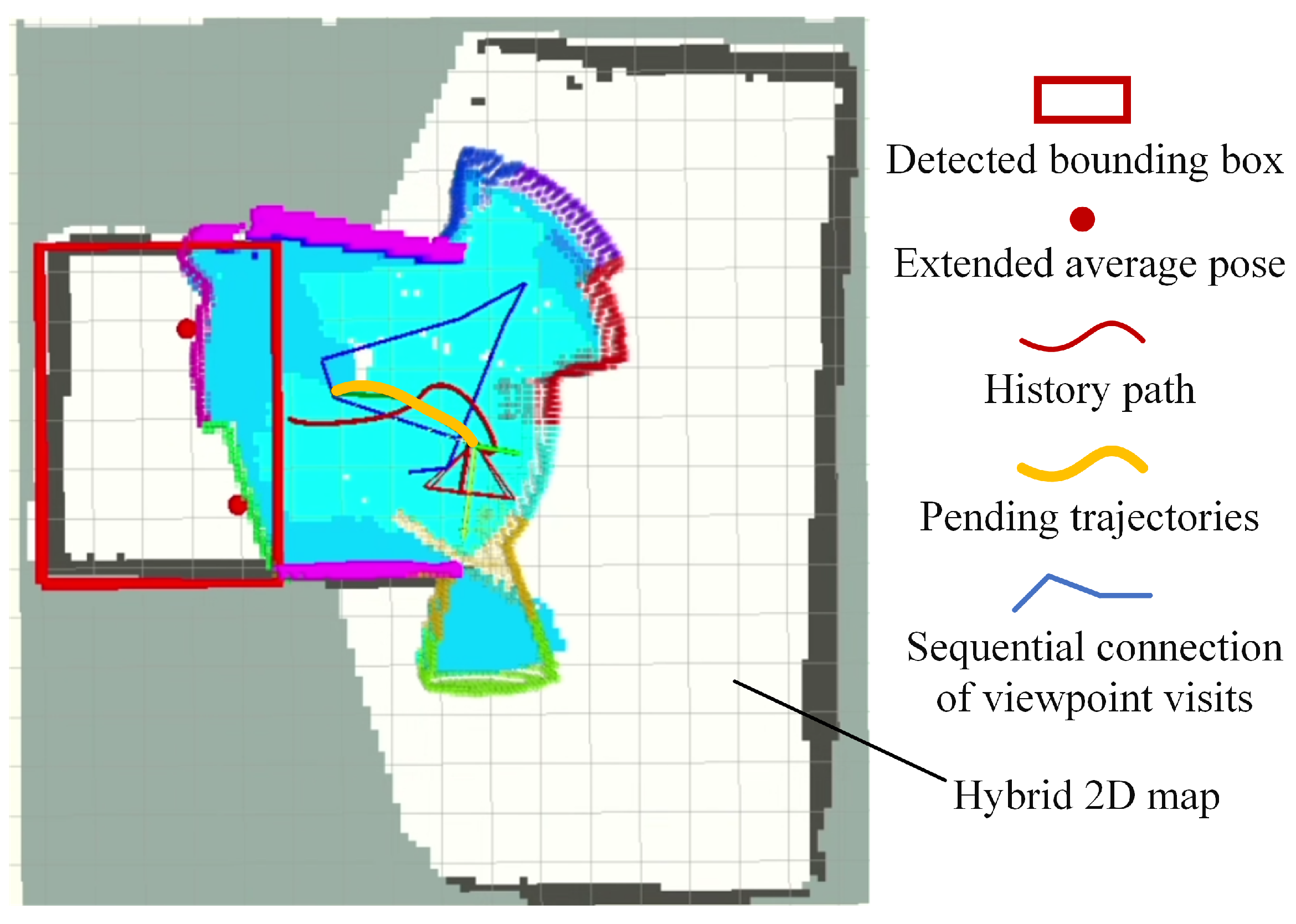
3.3.3. Isolated-Area Cluster Detection
3.3.4. Solving the ATSP
3.4. Motion Planning Module
| Algorithm 2 Path information gain optimization strategy. |
| Input: , , , , , , , Output: yaw Trajectory Y , , for each in do , if then , , end if end for if then return else return end if |
4. Experiments
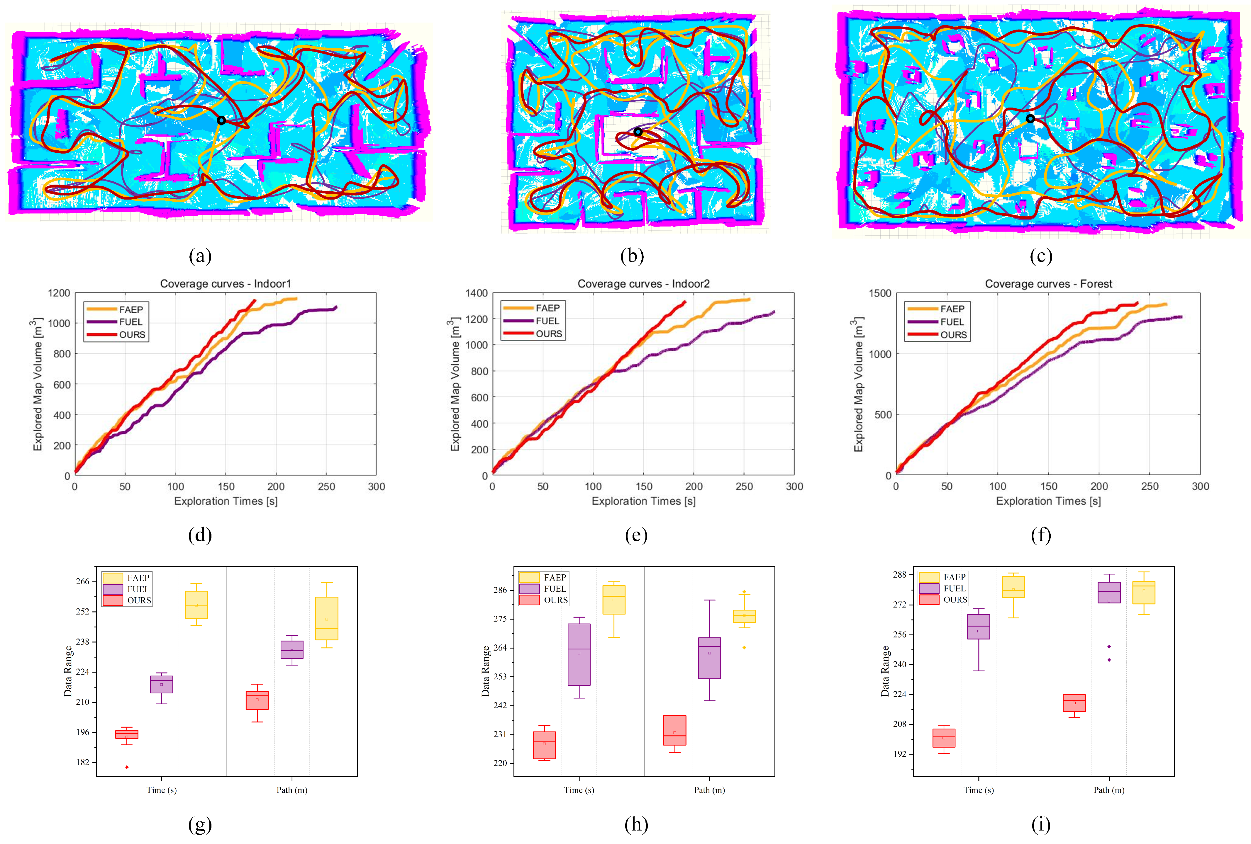
4.1. Simulations
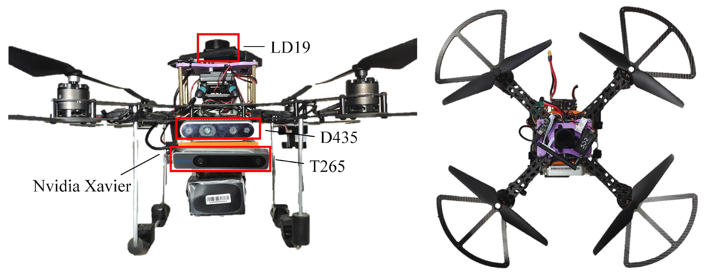
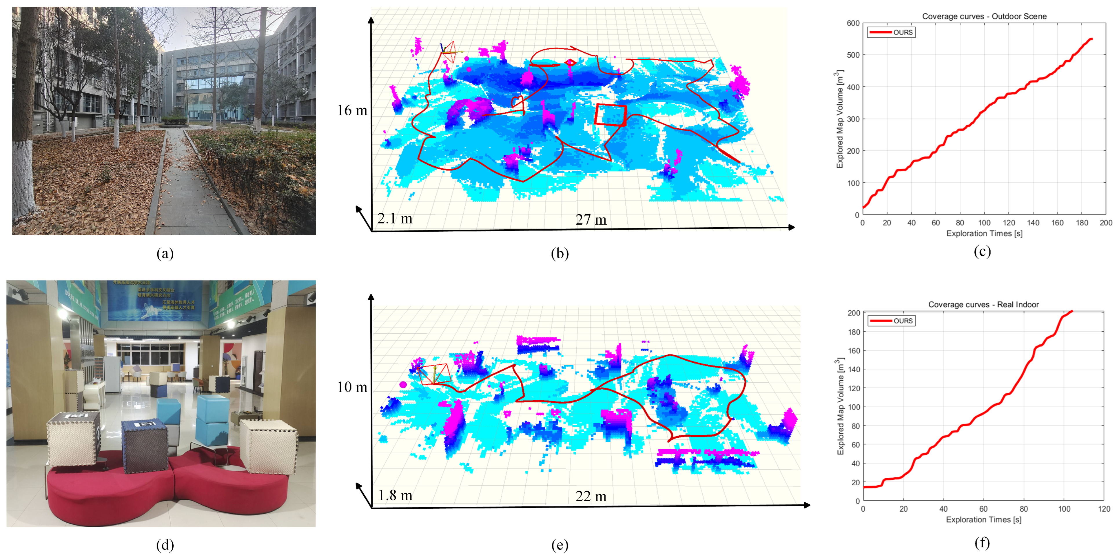
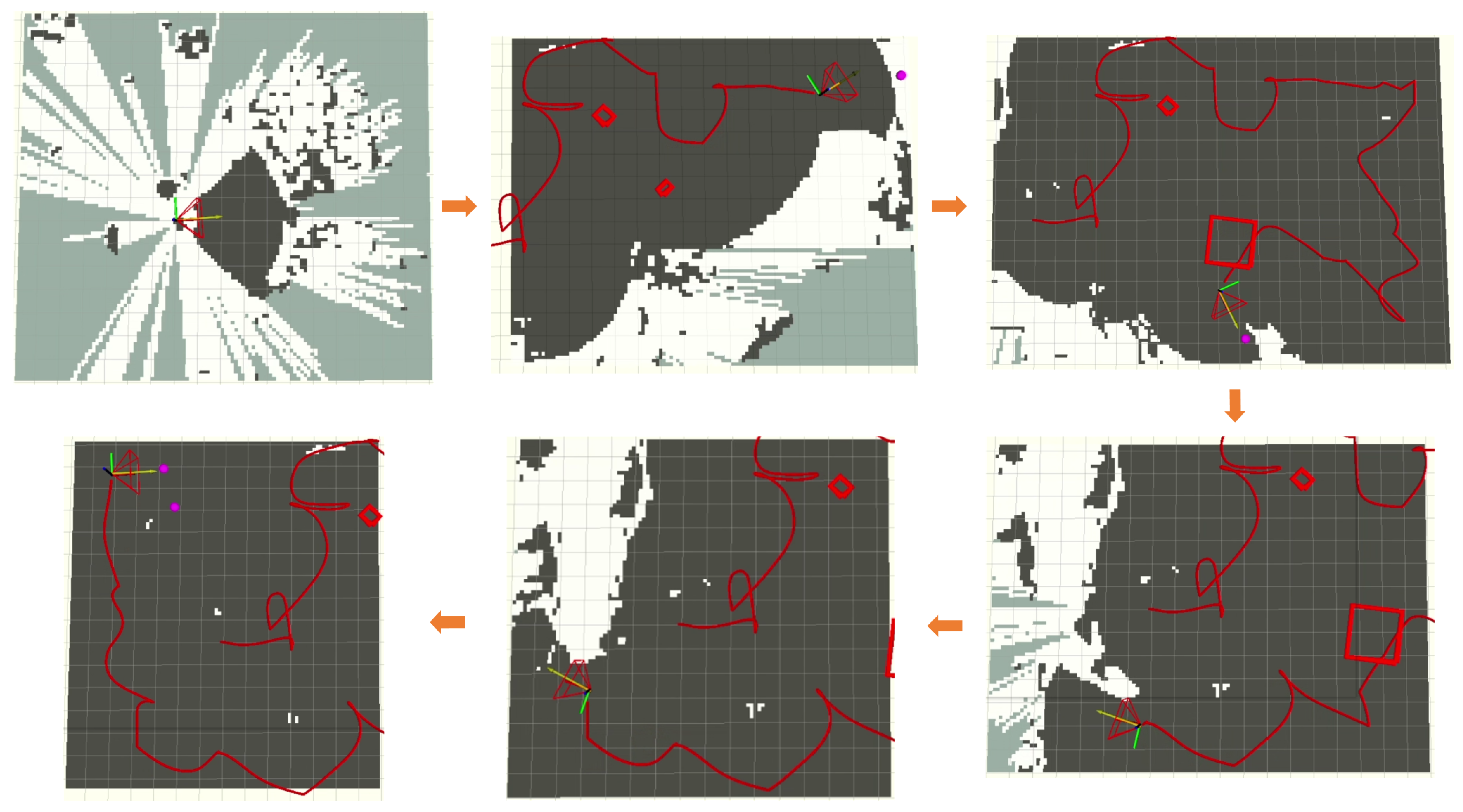
4.2. Real-World Experiments
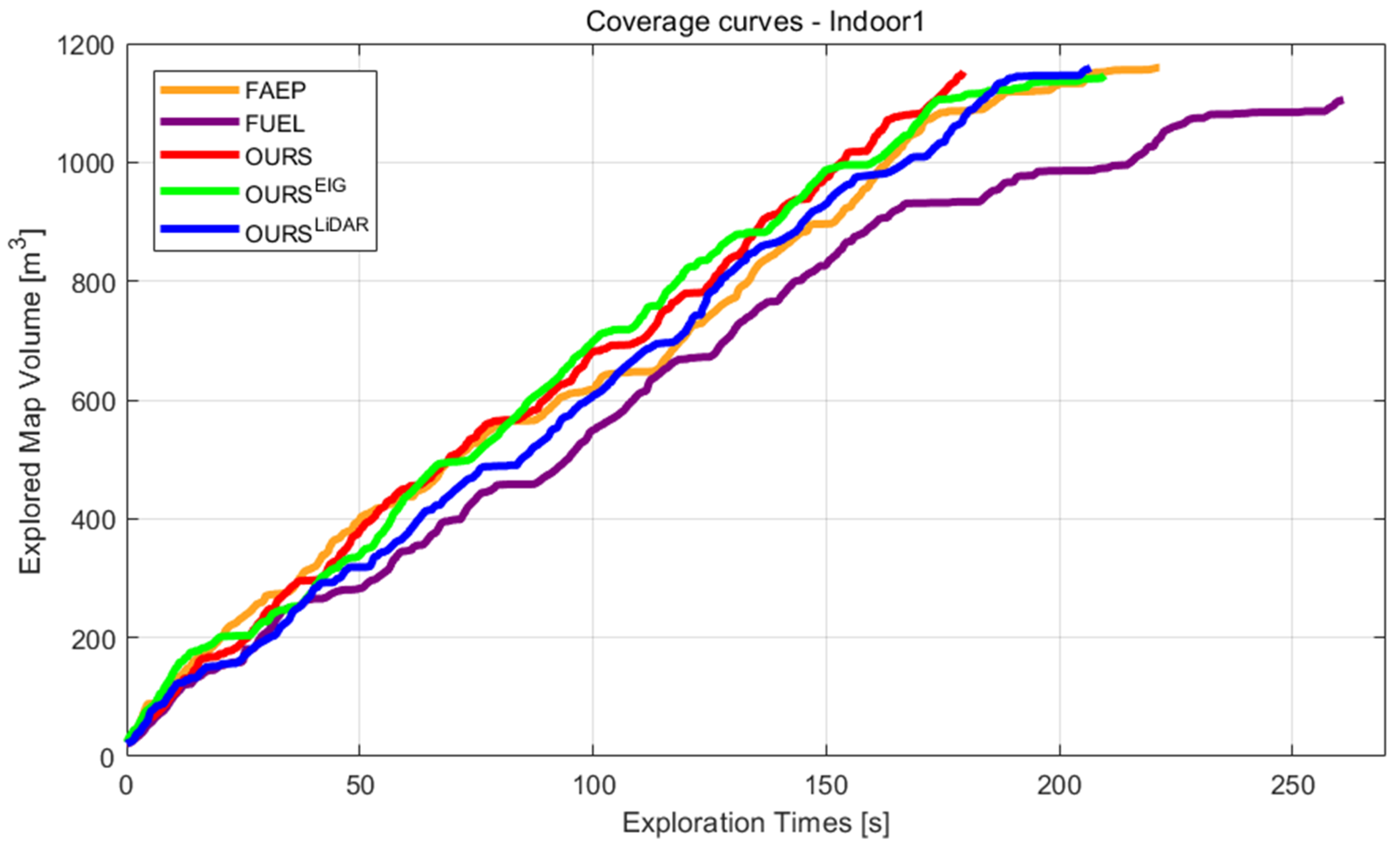
4.3. Discussion of the Use of LiDAR
5. Conclusions
Author Contributions
Funding
Data Availability Statement
Conflicts of Interest
References
- Siddiqui, Z.A.; Park, U. A drone based transmission line components inspection system with deep learning technique. Energies 2020, 13, 3348. [Google Scholar] [CrossRef]
- Yumin, Y. Research and design of high-precision positioning system for agricultural plant protection UAV—Based on GPS and GPRS. J. Agric. Mech. Res. 2016, 38, 227–231. [Google Scholar]
- Cho, S.W.; Park, H.J.; Lee, H.; Shim, D.H.; Kim, S.-Y. Coverage path planning for multiple unmanned aerial vehicles in maritime search and rescue operations. Comput. Ind. Eng. 2021, 161, 107612. [Google Scholar] [CrossRef]
- Duberg, D.; Jensfelt, P. Ufoexplorer: Fast and scalable sampling-based exploration with a graph-based planning structure. IEEE Robot. Autom. Lett. 2022, 7, 2487–2494. [Google Scholar] [CrossRef]
- Bircher, A.; Kamel, M.; Alexis, K.; Oleynikova, H.; Siegwart, R. Receding horizon “next-best-view” planner for 3d exploration. In Proceedings of the 2016 IEEE International Conference on Robotics and Automation (ICRA), Stockholm, Sweden, 16–21 May 2016; pp. 1462–1468. [Google Scholar]
- Dharmadhikari, M.; Dang, T.; Solanka, L.; Loje, J.; Nguyen, H.; Khedekar, N.; Alexis, K. Motion primitives-based path planning for fast and agile exploration using aerial robots. In Proceedings of the 2020 IEEE International Conference on Robotics and Automation (ICRA), Paris, France, 31 May–31 August 2020; pp. 179–185. [Google Scholar]
- Zhou, B.; Zhang, Y.; Chen, X.; Shen, S. Fuel: Fast uav exploration using incremental frontier structure and hierarchical planning. IEEE Robot. Autom. Lett. 2021, 6, 779–786. [Google Scholar] [CrossRef]
- Zhao, Y.; Yan, L.; Xie, H.; Dai, J.; Wei, P. Autonomous Exploration Method for Fast Unknown Environment Mapping by Using UAV Equipped with Limited FOV Sensor. IEEE Trans. Ind. Electron. 2023, 71, 4933–4943. [Google Scholar] [CrossRef]
- Tao, Y.; Wu, Y.; Li, B.; Cladera, F.; Zhou, A.; Thakur, D.; Kumar, V. Seer: Safe efficient exploration for aerial robots using learning to predict information gain. In Proceedings of the 2023 IEEE International Conference on Robotics and Automation (ICRA), London, UK, 29 May–2 June 2023; pp. 1235–1241. [Google Scholar]
- Umari, H.; Mukhopadhyay, S. Autonomous robotic exploration based on multiple rapidly-exploring randomized trees. In Proceedings of the 2017 IEEE/RSJ International Conference on Intelligent Robots and Systems (IROS), Vancouver, BC, Canada, 24–28 September 2017; pp. 1396–1402. [Google Scholar]
- Zhu, H.; Cao, C.; Xia, Y.; Scherer, S.; Zhang, J.; Wang, W. DSVP: Dual-stage viewpoint planner for rapid exploration by dynamic expansion. In Proceedings of the 2021 IEEE/RSJ International Conference on Intelligent Robots and Systems (IROS), Kyoto, Japan, 23–27 October 2021; pp. 7623–7630. [Google Scholar]
- Xu, Z.; Deng, D.; Shimada, K. Autonomous UAV exploration of dynamic environments via incremental sampling and probabilistic roadmap. IEEE Robot. Autom. Lett. 2021, 6, 2729–2736. [Google Scholar] [CrossRef]
- Xu, Z.; Suzuki, C.; Zhan, X.; Shimada, K. Heuristic-based Incremental Probabilistic Roadmap for Efficient UAV Exploration in Dynamic Environments. arXiv 2023, arXiv:2309.09121. [Google Scholar]
- Yamauchi, B. A frontier-based approach for autonomous exploration. In Proceedings of the 1997 IEEE International Symposium on Computational Intelligence in Robotics and Automation CIRA’97: Towards New Computational Principles for Robotics and Automation, Monterey, CA, USA, 10–11 July 1997; pp. 146–151. [Google Scholar]
- Kulich, M.; Faigl, J.; Přeučil, L. On distance utility in the exploration task. In Proceedings of the 2011 IEEE International Conference on Robotics and Automation, Shanghai, China, 9–13 May 2011; pp. 4455–4460. [Google Scholar]
- Kamalova, A.; Kim, K.D.; Lee, S.G. Waypoint mobile robot exploration based on biologically inspired algorithms. IEEE Access 2020, 8, 190342–190355. [Google Scholar] [CrossRef]
- Yu, J.; Shen, H.; Xu, J.; Zhang, T. ECHO: An Efficient Heuristic Viewpoint Determination Method on Frontier-based Autonomous Exploration for Quadrotors. IEEE Robot. Autom. Lett. 2023, 8, 5047–5054. [Google Scholar] [CrossRef]
- Amanatides, J.; Woo, A. A fast voxel traversal algorithm for ray tracing. Eurographics 1978, 87, 3–10. [Google Scholar]
- Helsgaun, K. An effective implementation of the Lin–Kernighan traveling salesman heuristic. Eur. J. Oper. Res. 2000, 126, 106–130. [Google Scholar] [CrossRef]
- Zhao, Y.; Yan, L.; Chen, Y.; Dai, J.; Liu, Y. Robust and efficient trajectory replanning based on guiding path for quadrotor fast autonomous flight. Remote Sens. 2021, 13, 972. [Google Scholar] [CrossRef]
- Faessler, M.; Franchi, A.; Scaramuzza, D. Differential flatness of quadrotor dynamics subject to rotor drag for accurate tracking of high-speed trajectories. IEEE Robot. Autom. Lett. 2017, 3, 620–626. [Google Scholar] [CrossRef]
- Han, L.; Gao, F.; Zhou, B.; Shen, S. Fiesta: Fast incremental euclidean distance fields for online motion planning of aerial robots. In Proceedings of the 2019 IEEE/RSJ International Conference on Intelligent Robots and Systems (IROS), Macau, China, 3–8 November 2019; pp. 4423–4430. [Google Scholar]
- Hornung, A.; Wurm, K.M.; Bennewitz, M.; Stachniss, C.; Burgard, W. OctoMap: An efficient probabilistic 3D mapping framework based on octrees. Auton. Robot. 2013, 34, 189–206. [Google Scholar] [CrossRef]
- LDRobot. Available online: https://www.ldrobot.com/ProductDetails?sensor_name=STL-19P (accessed on 1 January 2020).
- Shi, D.; Dai, X.; Zhang, X.; Quan, Q. A practical performance evaluation method for electric multicopters. IEEE/ASME Trans. Mechatron. 2017, 22, 1337–1348. [Google Scholar] [CrossRef]


| Data | Explanation |
|---|---|
| The extra information gain observed using LiDAR (m) | |
| Extension of average position of cluster by | |
| Cluster with low | |
| Another cluster tends to cause back-and-forth motion |
| Camera FOV | [80,60] deg | Camera range | 4.5 m |
| LiDAR FOV | 360 deg | LiDAR range | 12 m |
| Max velocity | 1.0 m/s | Max accelerate | 1.0 m/s2 |
| Max yaw rate | 1.0 rad/s | ROS version | Melodic |
| Hardware configuration | Intel Core i5-12500H@3.10 GHz, 16 GB memory | ||
| Scene | Method | Exploration Times (s) | Flight Distance (m) | ||||
|---|---|---|---|---|---|---|---|
| Avg | Std | Min | Avg | Std | Min | ||
| Indoor1 | FUEL [7] | 255.0 | 7.0 | 245.8 | 248.5 | 10.4 | 235.3 |
| FAEP [8] | 218.2 | 5.0 | 209.3 | 234.0 | 4.4 | 227.3 | |
| OURS | 193.8 | 5.1 | 179.9 | 211.1 | 5.1 | 200.9 | |
| 206.7 | 4.5 | 199.4 | 232.2 | 5.6 | 224.6 | ||
| 204.6 | 7.1 | 189.9 | 228.9 | 5.1 | 218.2 | ||
| Indoor2 | FUEL [7] | 280.1 | 7.1 | 265.0 | 279.6 | 7.5 | 266.8 |
| FAEP [8] | 257.9 | 11.0 | 236.7 | 274.0 | 14.6 | 242.6 | |
| OURS | 200.7 | 5.6 | 192.4 | 219.4 | 5.0 | 211.9 | |
| Forest | FUEL [7] | 282.3 | 6.3 | 268.1 | 276.4 | 5.7 | 264.2 |
| FAEP [8] | 262.1 | 10.7 | 244.9 | 262.1 | 12.0 | 243.9 | |
| OURS | 227.6 | 5.3 | 221.2 | 231.7 | 5.8 | 224.3 | |
Disclaimer/Publisher’s Note: The statements, opinions and data contained in all publications are solely those of the individual author(s) and contributor(s) and not of MDPI and/or the editor(s). MDPI and/or the editor(s) disclaim responsibility for any injury to people or property resulting from any ideas, methods, instructions or products referred to in the content. |
© 2024 by the authors. Licensee MDPI, Basel, Switzerland. This article is an open access article distributed under the terms and conditions of the Creative Commons Attribution (CC BY) license (https://creativecommons.org/licenses/by/4.0/).
Share and Cite
Hou, X.; Pan, Z.; Lu, L.; Wu, Y.; Hu, J.; Lyu, Y.; Zhao, C. LAEA: A 2D LiDAR-Assisted UAV Exploration Algorithm for Unknown Environments. Drones 2024, 8, 128. https://doi.org/10.3390/drones8040128
Hou X, Pan Z, Lu L, Wu Y, Hu J, Lyu Y, Zhao C. LAEA: A 2D LiDAR-Assisted UAV Exploration Algorithm for Unknown Environments. Drones. 2024; 8(4):128. https://doi.org/10.3390/drones8040128
Chicago/Turabian StyleHou, Xiaolei, Zheng Pan, Li Lu, Yuhang Wu, Jinwen Hu, Yang Lyu, and Chunhui Zhao. 2024. "LAEA: A 2D LiDAR-Assisted UAV Exploration Algorithm for Unknown Environments" Drones 8, no. 4: 128. https://doi.org/10.3390/drones8040128
APA StyleHou, X., Pan, Z., Lu, L., Wu, Y., Hu, J., Lyu, Y., & Zhao, C. (2024). LAEA: A 2D LiDAR-Assisted UAV Exploration Algorithm for Unknown Environments. Drones, 8(4), 128. https://doi.org/10.3390/drones8040128