Extending Conflict-Based Search for Optimal and Efficient Quadrotor Swarm Motion Planning

Abstract

Multi-agent pathfinding has been extensively studied by the robotics and artificial intelligence communities. The classical algorithm, conflict-based search (CBS), is widely used in various real-world applications due to its ability to solve large-scale conflict-free paths. However, classical CBS assumes discrete time–space planning and overlooks physical constraints in actual scenarios, making it unsuitable for direct application in unmanned aerial vehicle (UAV) swarm. Inspired by the decentralized planning and centralized conflict resolution ideas of CBS, we propose, for the first time, an optimal and efficient UAV swarm motion planner that integrates state lattice with CBS without any underlying assumption, named SL-CBS. SL-CBS is a two-layer search algorithm: (1) The low-level search utilizes an improved state lattice. We design emergency stop motion primitives to ensure complete UAV dynamics and handle spatio-temporal constraints from high-level conflicts. (2) The high-level algorithm defines comprehensive conflict types and proposes a motion primitive conflict detection method with linear time complexity based on Sturm’s theory. Additionally, our modified independence detection (ID) technique is applied to enable parallel conflict processing. We validate the planning capabilities of SL-CBS in classical scenarios and compare these with the latest state-of-the-art (SOTA) algorithms, showing great improvements in success rate, computation time, and flight time. Finally, we conduct large-scale tests to analyze the performance boundaries of SL-CBS+ID.

1. Introduction

Swarm motion planning is a fundamental technology for the autonomous flight of unmanned aerial vehicle (UAV) swarm, aiming to solve a dynamically feasible and collision-free flight trajectory for each one. Based on the organizational structure of the swarm, swarm motion planning generally employs either centralized or decentralized methods. Centralized methods struggle to provide feasible solutions within a limited time due to the curse of dimensionality [1]. In contrast, decentralized methods plan independently, offering fast computation but often lacking optimality, resulting in poor solution quality and potential deadlocks (especially in symmetrical scenarios) [2,3]. Balancing optimality, high-quality solutions, and computational efficiency remains an unresolved challenge in swarm motion planning.

A simplified problem corresponding to swarm motion planning in discrete time–space is multi-agent PathFinding (MAPF). MAPF is an NP-hard graph search problem that seeks to find multiple conflict-free paths [4]. The classical algorithm conflict-based search (CBS) and its variants have made great progress in recent years and have been widely applied in fields such as warehouse management, airport towing, and railway planning [5]. CBS consists of two layers: the low-level algorithm plans a collision-free path for each agent in a decentralized manner, like A* or SIPP (safe interval path planning). The high-level algorithm centrally detects conflicts among all paths and resolves them by imposing constraints at the low level, iterating until no conflicts are found [6]. However, due to the movement constraints of agents in MAPF and various physical assumptions, such as 4/8-neighbors search space and waiting at the same location, CBS is difficult to directly apply to robots like UAVs that require continuous motion planning.

Inspired by the CBS algorithm for solving MAPF, its decentralized planning and centralized conflict resolution provide a new approach for UAV swarm motion planning. By enhancing the low-level discrete path planning to continuous motion planning that accounts for UAV dynamics, defining new conflict types and implementing conflict detection methods at the high level, the CBS can be extended to swarm motion planning.

Similarly, we integrate state lattice with CBS to propose an optimal and efficient swarm motion planner suitable for a quadrotor swarm, named SL-CBS. The SL-CBS algorithm is also divided into two layers. The low-level is an improved state lattice based on motion primitive search. To implement waiting actions, we design an emergency stop motion primitive. Additionally, we handle spatio-temporal constraints from high-level conflict resolution. At the high level, we define comprehensive conflict types, particularly motion primitive conflicts. Instead of sampling in the time dimension for conflict detection, we propose a linear complexity conflict detection method based on Sturm’s theory. Additionally, our modified independent detection (ID) technology applied to the SL-CBS provides the ability to parallel process conflicts, enhancing planning ability in certain scenarios. Our main contributions are as follows:

(1)

We extend the CBS algorithm to quadrotor swarm motion planning and propose the optimal and efficient SL-CBS planner integrating state lattice and CBS.

(2)

At the low-level, we improve state lattice based on motion primitive search that considers a complete dynamic model. We design emergency stop motion primitives and address the corresponding spatio-temporal constraints.

(3)

At the high-level, we define motion primitive conflicts and propose a conflict detection method with linear time complexity based on Sturm’s theory.

(4)

We validate the planning capabilities of SL-CBS in classical scenarios such as CrossAndSwap, Cross and Swap.

(5)

The benchmarks are designed and compared to the latest state-of-the-art (SOTA) algorithms, and SL-CBS demonstrates higher success rates, reduced computation time, and lower flight costs.

(6)

We analyze the performance boundaries of SL-CBS+ID in large-scale batch testing.

2. Related Work

2.1. MAPF

Consider an undirected graph $G\left(V,E\right)$, where V represents vertices and E represents edges connecting two vertices, assuming a set of K agents $\left\{a_1,a_2,\dots ,a_K\right\}$ with starting positions $s=\left(s_1,s_2,\dots ,s_K\right)$ and goal positions $g=\left(g_1,g_2,\dots ,g_K\right)$, where $s_i\in V$ and $g_i\in V$ for $1\le i\le K$. Time is discretized as $t=1,2,\dots$. At each time step, agents can perform one of two actions: move to a neighboring node (4/8-neighbors) or wait at their current position. Each action incurs a unit cost of 1. The objective of MAPF is to determine conflict-free paths for each agent while minimizing the total travel cost. Conflicts typically fall into two categories: vertex conflicts and edge conflicts. A vertex conflict $〈a_i,a_j,v_i,v_j,t〉$ indicates that agents $a_i$ and $a_j$ are in conflict at positions $v_i$ and $v_j$, respectively, at time t, typically with $v_i=v_j$. An edge conflict $〈a_i,a_j,v_i,v_{i+1},v_j,v_{j+1},t〉$ occurs when agent $a_i$ moves from $v_i$ to $v_{i+1}$ and agent $a_j$ moves from $v_j$ to $v_{j+1}$ at time t, typically with $v_i=v_{j+1}$ and $v_{i+1}=v_j$.

2.2. CBS and Its Developments

The main methods for solving the MAPF include A*-based methods, reduction-based methods, ICTS (increasing cost tree search) and CBS, with detailed reviews in [7,8]. In recent years, the CBS algorithm has attracted significant interest from researchers and scholars due to its powerful conflict resolution capabilities and large-scale conflict-free paths planning abilities.

CBS is a two-layer search algorithm, and its detailed process can be found in [6]. The low-level finds optimal paths for each agent that satisfy spatio-temporal constraints, often using the A* algorithm. The high-level maintains a constraint tree $CT$, where each node $N\in CT$ consists of three components: (1) a set of constraints applied to the agents, $N.constraints$; (2) a set of solutions satisfying all constraints, $N.solutions$; (3) the cost of the solutions, $N.cost$. The root node of the $CT$ is constructed from the solutions of single-agent planning without constraints, and the optimal node is selected for expansion based on a greedy search strategy. After selecting a node for expansion, the high-level algorithm checks for conflicts among the agents. If no conflicts exist, the current node is considered as the goal node, and the high-level algorithm terminates, returning the solutions. Otherwise, CBS selects a conflict to resolve, such as $〈a_i,a_j,v_i,v_j,t〉$. Two child nodes are created, inheriting the parent node’s constraints. Then, constraints $〈a_i,v_i,t〉$ and $〈a_j,v_j,t〉$ are added to each child node, respectively. The constraint $〈a_i,v_i,t〉$ prohibits agent $a_i$ from moving to vertex $v_i$ at time t, and similarly for $〈a_j,v_j,t〉$. After adding constraints, the child nodes are replanned using the low-level algorithm and added to the $CT$.

Subsequent developments in CBS have been significant. Ref. [9] classifies conflicts among agents into cardinal, semi-cardinal, and non-cardinal conflicts, prioritizing the resolution of cardinal conflicts. For semi-cardinal and non-cardinal conflicts, agents with alternative paths of equal cost are rerouted to bypass conflicts [10]. In [11,12], the symmetry-breaking technique and weighted dependency graph heuristic are proposed for four-connected grid maps, solving paths for hundreds of agents in dense maps.

2.3. Swarm Motion Planning Using CBS

In existing work, the CCBS (continuous-time CBS) algorithm proposed in [13] is an attempt to extend CBS to real-world robots. It defines state conflict types that consider the geometric sizes of robots in the high-level algorithm and computes unsafe time intervals. The low-level search uses the SIPP for continuous time planning to handle unsafe time interval constraints. Although in subsequent works, ICCBS (improved CCBS) [14] and CCBS-PGA (CBS with partitioned groups of agents) [15] employ techniques like prioritizing conflicts (PCs), disjoint splitting (DC), high-level heuristics (HH), and prioritized planning (PP) to reduce computing time, they are limited to disc robots and have many physical constraints, such as simple motion models, constant velocity, and ignoring inertia. The CBS-MP (CBS motion planning) proposed in [16] constructs a roadmap using the PRM (probabilistic RoadMap) sampling algorithm during preprocessing, providing feasible paths for all agents. Although roadmap-based CBS efficiently solves paths, the low-level algorithm does not consider dynamic and kinematic models, making the paths suitable only for discrete motion operators.

The work in [17] first integrates the CBS with the hybrid-state A* algorithm considering dynamics, proposing the CL-CBS (car-like CBS) for Ackermann-steering vehicles. However, the low-level hybrid-state A* requires vehicles to move at constant speed, accelerate instantly to constant speed, and brake instantly, which is unrealistic. Moreover, the CBS high level only considers state conflicts between vehicles, ignoring motion primitive conflicts, leading to a lack of safety guarantees. Although in a subsequent work HG-CBS (heuristic group-based CBS) [18] improves computational efficiency through grouping and improved search strategies, it does not overcome the original issues. The K-CBS (Kinodynamic CBS) proposed in [19] uses a sampling algorithm considering full dynamics for low-level planning, with high-level algorithms performing state conflict detection after uniform time sampling to determine conflict intervals. Although its multiple motion trajectory results are suitable for real-world swarm motion scenarios, inefficient conflict detection and single-agent planning limit its scalability. In [20], CB-MPC (conflict-based model predictive control) fully considers the dynamic and kinematic models of nonlinear unicycles, using an MPC optimal controller for CBS’s low-level algorithm. It solves multiple motion trajectories for complex scenarios through iterative continuous planning, but the large computational load and long optimization time of the MPC optimal control problem result in low overall computational efficiency. The latest db-CBS (discontinuity-bounded CBS) [21] implements low-level planning based on db-A* [22], which pre-solves two-point boundary value problems to compute motion primitives meeting dynamic requirements, followed by bounded discontinuous A* search for motion trajectories. Outside the CBS’s two-layer algorithm, db-CBS designs a multi-robot trajectory optimization layer to address bounded discontinuities in low-level planning. db-CBS efficiently solves large-scale swarm motion trajectories but relies on the time-consuming offline pre-computation of motion primitives.

The aforementioned works, Refs. [13,14,15,16] do not consider a comprehensive kinematic and dynamic model for robots. Refs. [17,18] lack safety guarantees, refs. [19,20] suffer from low computational efficiency, and ref. [21] requires an offline pre-computation process. Our aim is to overcome all these existing issues by following the CBS framework to propose an online, complete, optimal, and efficient UAV swarm motion planner that accounts for full dynamics.

The organization of this paper is as follows: Section 3 formally defines the UAV swarm motion planning problem. In Section 4, we introduce the SL-CBS+ID algorithm framework and its corresponding components. Section 5 presents the experimental results, including tests on classical scenarios, comparisons with baseline algorithms, and performance boundary analysis. Finally, Section 6 provides a summary of the work and suggests potential future research directions.

3. Problem Description

The UAV swarm consists of K identical quadrotors, operating within a workspace W, where $W\subset R^m$ and $m=2,3$. Given an obstacle space $P^{obs}$, the free space is defined as $P^{free}=W\setminus P^{obs}$.

The state of $UA{V}_i$ is represented as $x_i\left(t\right)={\left[p_i^T\left(t\right),v_i^T\left(t\right),\dots ,p_i^{{\left(q-1\right)}^T}\left(t\right)\right]}^T$, where $x_i\left(t\right)\in \chi \subset R^{mq}$, $1\le i\le K$, and $\chi$ is the state space. The state $x_i\left(t\right)$ includes the UAV’s position $p_i\left(t\right)$, velocity $v_i\left(t\right)$ and the derivatives up to order $q-1$. The q-th derivative of $p_i\left(t\right)$ is the control input $u_i\left(t\right)$, where $u_i\left(t\right)=p_i^{\left(q\right)}\left(t\right)$, and $u_i\left(t\right)\in U:={[-u_{max},u_{max}]}^m$, with $u_{max}$ being the maximum control input. The UAVs follow the system model:

$$\dot{x}=Ax+Bu$$

(1)

where

$$A={\left[\begin{array}{ccccc}0& I_m& 0& \cdots & 0\\ 0& 0& I_m& \cdots & 0\\ ⋮& \ddots & \ddots & \ddots & ⋮\\ 0& \cdots & \cdots & 0& I_m\\ 0& \cdots & \cdots & 0& 0\end{array}\right]}_{qm\times qm},B={\left[\begin{array}{c}0\\ 0\\ ⋮\\ 0\\ I_m\end{array}\right]}_{qm\times m}$$

UAVs are subject to kinematic constraints such as maximum velocity $v_{max}$ and maximum acceleration $a_{max}$. The safe state space ${\chi }^{free}$ is defined as:

$${\chi }^{free}=P^{free}\times {\left[-v_{max},v_{max}\right]}^m\times {\left[-a_{max},a_{max}\right]}^m\times \dots$$

(2)

Additionally, $UA{V}_i$ is modeled as a rigid body, with $S\left(x_i\right)$ representing the workspace occupied by the $UA{V}_i$ in state $x_i\left(t\right)$. The UAV is geometrically modeled as a circle or sphere with its center at the UAV’s centroid and radius $r_c$.

The UAV swarm motion planning problem is described as follows: given each initial state $x_{i0}\in {\chi }^{free}$ for $UA{V}_i$, the goal is to reach the target region $X_i^G\subset {\chi }^{free}$. Within the given control input U, design the control input $u_i\left(t\right)$ for each UAV, adhering to the system model (1) and kino-dynamic constraints (2), to obtain the trajectory $T_i\left(t\right)$ such that $T_i\left(t_0\right)=x_{i0}$ and $T_i\left(t_{fi}\right)\in X_i^G$, where $t_0$ is the initial time of the swarm and $t_{fi}$ is the arrival time for $UA{V}_i$. The trajectories $T_1,T_2,\dots ,T_K$ must be conflict-free at any time t, meaning:

$$S\left(T_i\left(t\right)\right)\cap S\left(T_j\left(t\right)\right)=\mathrm{\varnothing },\hspace{1em}\forall 1\le i<j\le K$$

(3)

$$S\left(T_i\left(t\right)\right)\cap P^{obs}=\varnothing ,\hspace{1em}\forall 1\le i\le K$$

(4)

4. Algorithm

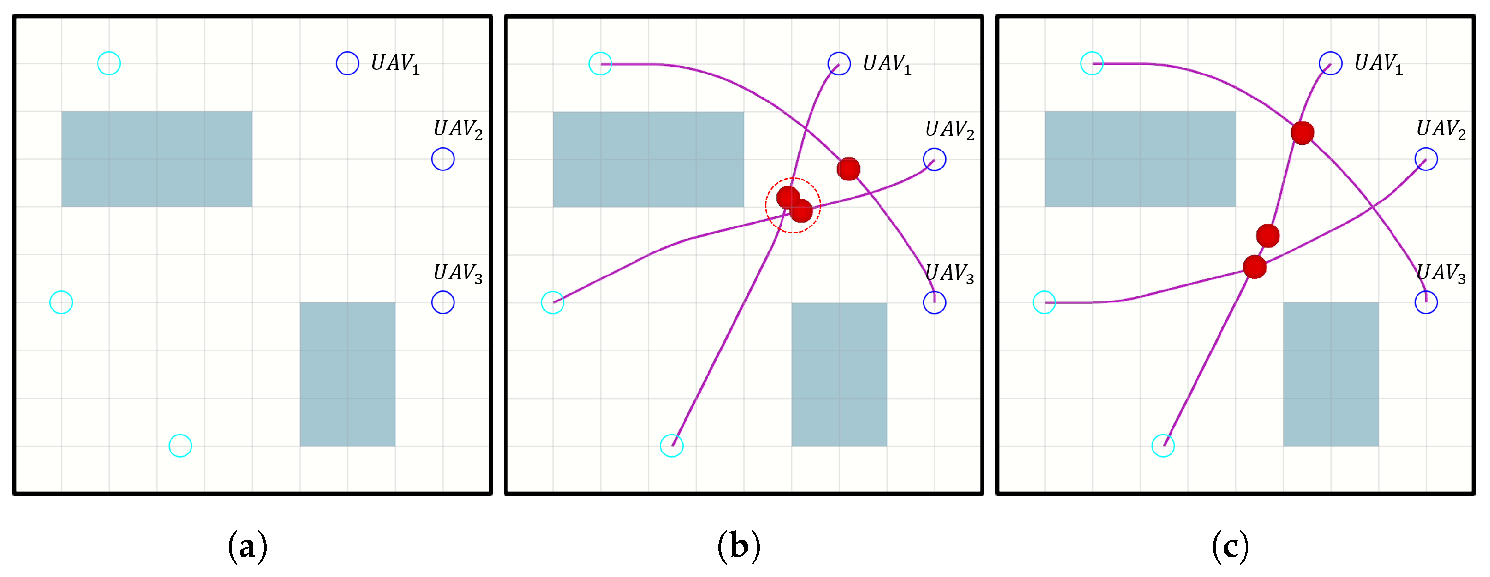
The SL-CBS algorithm builds upon the classic CBS framework, defining two conflict types: state conflicts and motion primitive conflicts. The low-level employs a state lattice algorithm based on motion primitive search to effectively handle spatio-temporal constraints, while the high-level introduces a conflict detection method based on Sturm’s theory and implements conflict resolution. Figure 1 clearly illustrates the planning process of the SL-CBS algorithm. Figure 1a depicts the initial state of a UAV swarm consisting of three UAVs, showcasing a map with obstacles, as well as the initial positions and target regions of the UAV swarm. Figure 1b presents the planning result of the first iteration of SL-CBS, where each UAV independently plans its trajectory without considering constraints. A collision occurs between the flight trajectories of $UA{V}_1$ and $UA{V}_2$. Figure 1c shows the planning result of the second iteration. After detecting the conflict in the higher-level algorithm, SL-CBS applies the corresponding constraints to the relevant UAVs and replans the trajectories. It can be observed that the three flight trajectories are now collision-free. The flight trajectories of $UA{V}_1$ and $UA{V}_3$ remain unchanged from Figure 1b, while $UA{V}_2$’s trajectory is replanned with the necessary constraints applied to avoid the collision detected in Figure 1b.

4.1. Definition of Two Conflict Types

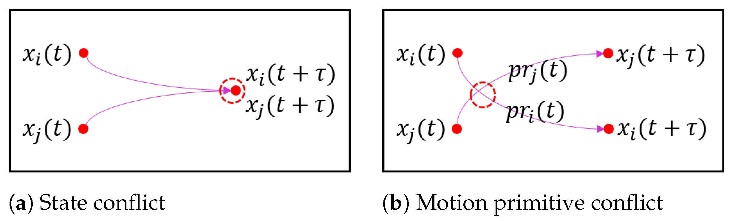
We comprehensively define two conflict types: state conflicts and motion primitive conflicts, addressing the limitation in [17] which only considers state conflicts. As shown in Figure 2, a state conflict, corresponding to a vertex conflict in the MAPF problem, is denoted as $〈x_i\left(t\right),x_j\left(t\right),t+\tau 〉$, indicating a conflict between the states $x_i(t+\tau )$ of $UA{V}_i$ and $x_j(t+\tau )$ of $UA{V}_j$ occurring at time $t+\tau$. A motion primitive conflict, also akin to an edge conflict in MAPF, is represented as $〈x_i\left(t\right),x_j\left(t\right),{pr}_i\left(t\right),{pr}_j\left(t\right),t,t+\tau 〉$, indicating a conflict between the motion primitive segment $p{r}_i\left(t\right)$ of $UA{V}_i$ and $p{r}_j\left(t\right)$ of $UA{V}_j$ over the interval $(t,t+\tau )$. The exact time and location of the conflict require precise calculation, but it occurs within $(t,t+\tau )$. A detailed description of motion primitive segments $p{r}_i\left(t\right)$ and $p{r}_j\left(t\right)$ is defined in Section 4.2.

After detecting conflicts and selecting one for resolution, the selected conflict is divided into specific constraints for the low-level algorithm to handle. A state conflict, $〈x_i\left(t\right),x_j\left(t\right),t+\tau 〉$, can be divided into constraints $〈UA{V}_i,\overline{x_j\left(t\right)},t+\tau 〉$ and $〈UA{V}_j,\overline{x_i\left(t\right)},t+\tau 〉$, where $〈UA{V}_i,\overline{x_j\left(t\right)},t+\tau 〉$ prohibits $UA{V}_i$ from reaching the vicinity of state $x_j\left(t\right)$ at time $t+\tau$, and similarly for $〈UA{V}_j,\overline{x_i\left(t\right)},t+\tau 〉$. A motion primitive conflict, $〈x_i\left(t\right),x_j\left(t\right),{pr}_i\left(t\right),{pr}_j\left(t\right),t,t+\tau 〉$, can be divided into constraints $〈UA{V}_i,\overline{{pr}_j\left(t\right)},t,t+\tau 〉$ and $〈UA{V}_j,\overline{{pr}_i\left(t\right)},t,t+\tau 〉$, where $〈UA{V}_i,\overline{{pr}_j\left(t\right)},t,t+\tau 〉$ prohibits $UA{V}_i$ from conflicting with motion primitive $p{r}_j\left(t\right)$ during $(t,t+\tau )$, and similarly for $〈UA{V}_j,\overline{{pr}_i\left(t\right)},t,t+\tau 〉$.

4.2. Improved State Lattice

State lattice is a motion planning method based on motion primitive search, integrating the advantages of considering UAV dynamics and A* search [23]. The state lattice algorithm first uniformly samples each dimension of the control input U over $[0,u_{max}]$ with a sampling number $\mu$, generating a control input sample set $U_M:=\left\{u_1,u_2,\dots ,u_M\right\}$, where $M={(2\mu +1)}^3$. Given the initial state $x_0:={\left(p_0^T,v_0^T,a_0^T,\dots \right)}^T$, time interval $t>0$, and control input $u_m$, the motion primitive $pr\left(t\right)$ is generated based on the UAV system model (1):

$$pr\left(t\right)=x\left(t\right)=e^{At}{x}_0+\left[{\int }_0^t{e}^{A\left(t-\sigma \right)}Bd\sigma \right]u_m$$

(5)

The state transition equation $x\left(t\right)$ is represented by $pr\left(t\right)$ for clarity. According to [23], the motion primitive $pr\left(t\right)$ is a polynomial curve of the order $2q-1$. Similarly, we design the motion primitive cost J as follows:

$$J=J_s+\rho T=\underset{0}{\overset{T}{\int }}{∥u\left(t\right)∥}^{2}dt+\rho T$$

(6)

It is a linear combination of the smoothness cost $J_s$ and time cost T (note that, here, T refers to the time interval of the motion primitive as described in [23]). Assuming the time interval $t=\tau$, the motion primitive cost is $\left({∥u_m∥}^2+\rho \right)\tau$, where $\rho$ is the time cost weight. After constructing the motion primitive graph, the final trajectory is searched using the A* algorithm.

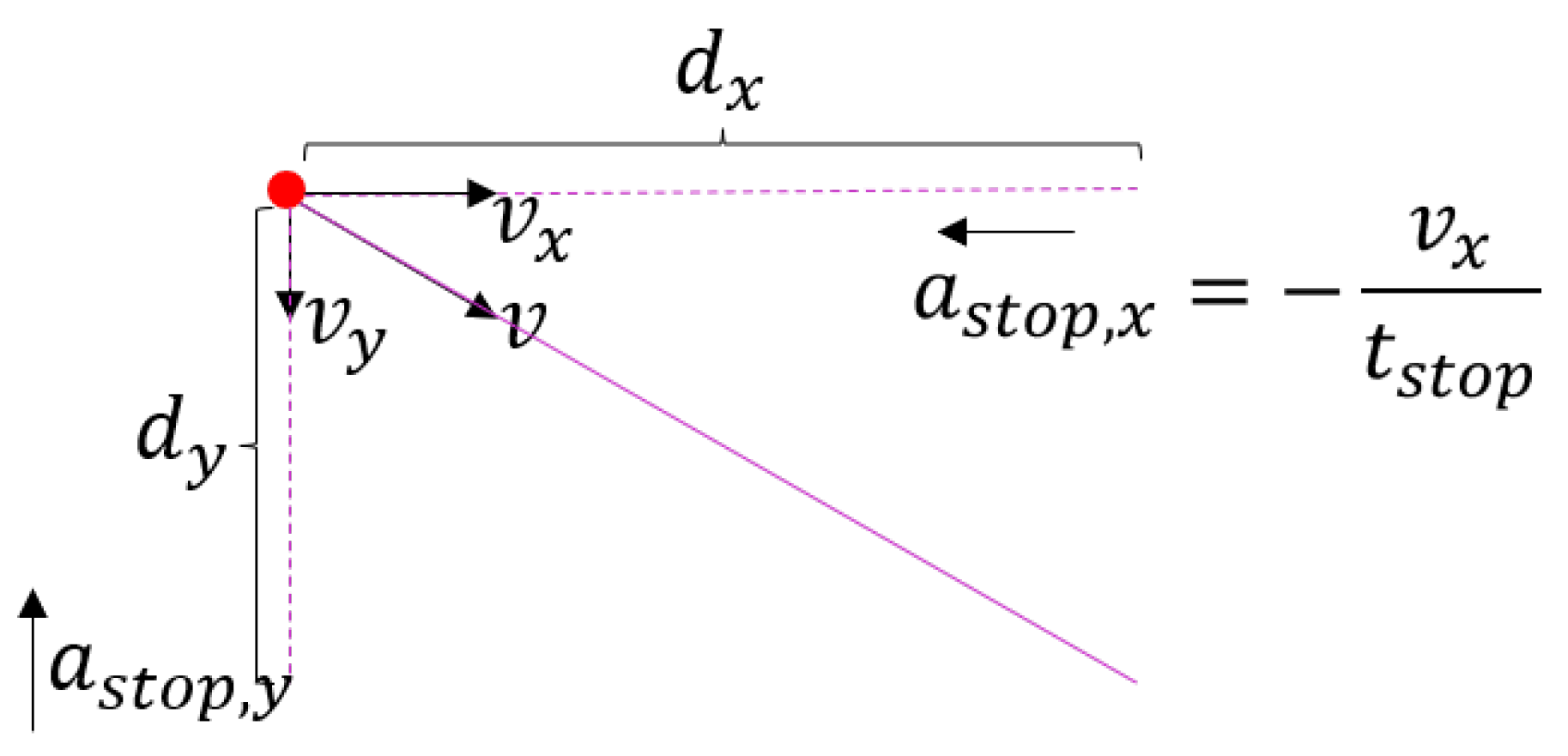
4.2.1. Emergency Stop Motion Primitive

In MAPF, the wait action is crucial, offering more possibilities in the motion space. When extended to UAV motion planning, an emergency stop motion primitive corresponding to the wait action is needed. Most existing work assumes that robots can stop instantaneously. However, we design an emergency stop motion primitive based on a maximum acceleration braking model, which is implemented through the three following steps: (1) Calculate the maximum braking time $t_{stop}$:

$$t_{stop}={\displaystyle \frac{{∥vs.∥}_{\infty }}{\lambda a_{max}}}$$

(7)

Here, $\lambda$ is a factor adjusting braking intensity to ensure completion within $\tau$; (2) Calculate braking acceleration:

$$a_{stop}=-{\displaystyle \frac{v}{t_{stop}}}=-{\displaystyle \frac{\lambda v{a}_{max}}{{∥vs.∥}_{\infty }}}$$

(8)

(3) For each axis, calculate the emergency stop motion primitive $p{r}_{stop}$ based on the braking model $d_i$:

$$d_i={\displaystyle \frac{v_i^2}{2a_{stop,i}}}$$

(9)

where $d_i$ is the displacement vector of braking distance in different dimensions. Taking a 2D workspace as an example, $i\in \left\{x,y\right\}$, as shown in Figure 3. The cost of the emergency stop motion primitive is designed as $J_{stop}=\rho \tau$, assuming no control input effect.

4.2.2. Spatio-Temporal Constraints

The high-level algorithm defines state and motion primitive conflicts, dividing them into specific state and motion primitive constraints. In the improved state lattice algorithm, these constraints are processed to prevent corresponding conflicts. The legality detection process after motion primitive generation involves two steps: (1) Check whether the constraint occurrence time overlaps with the current expanded state/motion primitive time. If not, skip the check; otherwise, proceed to (2); (2) For state constraints, check whether the current state conflicts with the constrained state. For motion primitive constraints, check whether the current motion primitive conflicts with the constrained motion primitive. The specific detection method is detailed in the conflict detection scheme in Section 4.3.

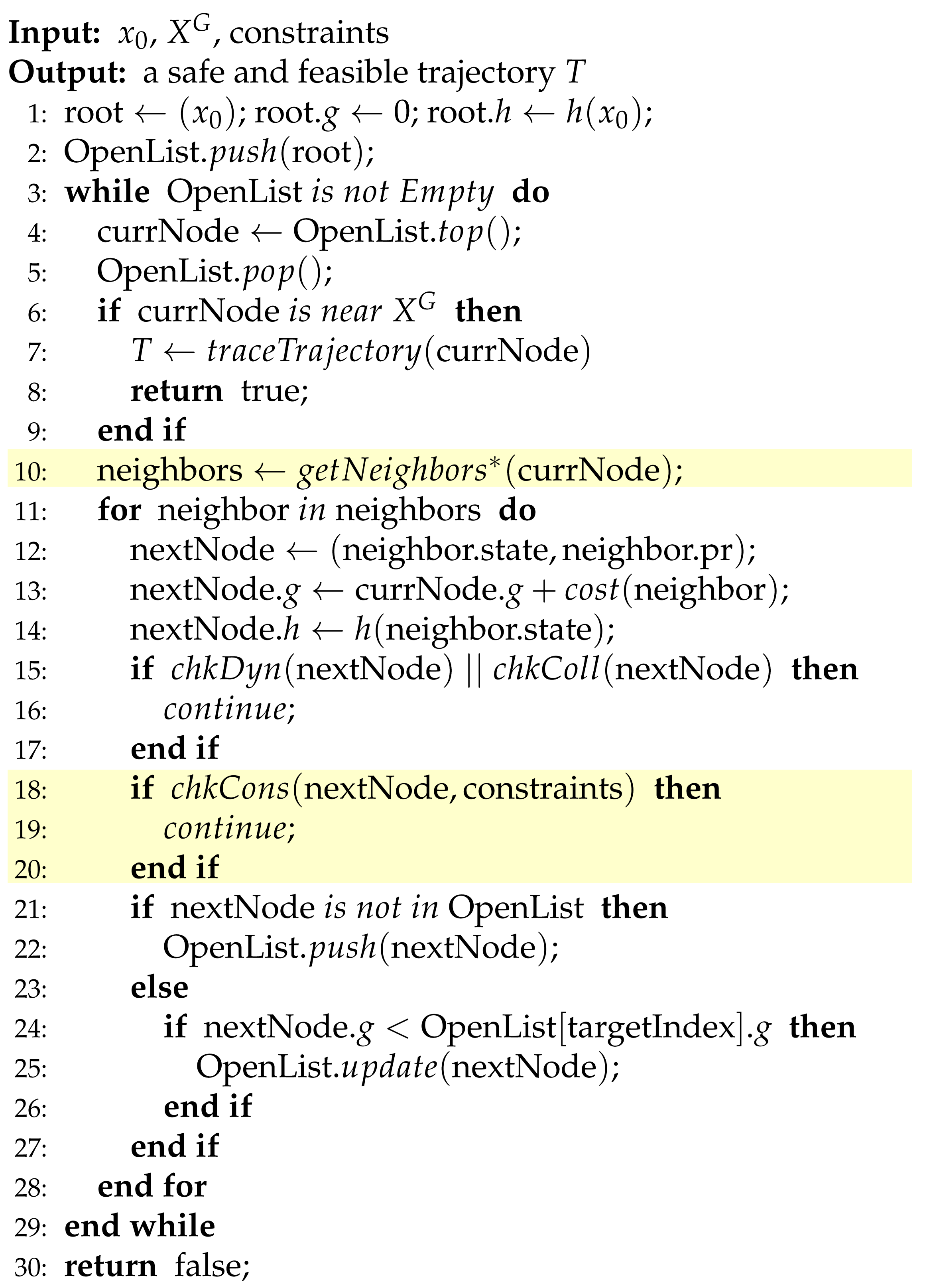
The improved state lattice pseudo-code is shown in Algorithm 1, with major improvements marked with light yellow areas, while the rest remains consistent with the original algorithm. In line 10, the $getNeighbor{s}^{*}$ function includes the design of emergency stop motion primitives, and lines 18–20 add a new check for potential violations of high-level constraints with $chkCons\left(\right)$.

Algorithm 1 Improved SLPlanner

4.3. Conflict Detection Method Based on Sturm’s Theory

Detecting state and motion primitive conflicts is a frequent operation that directly impacts the efficiency of swarm motion planning. State conflict detection can be directly performed using the geometric model and pose information of the UAVs. Given that $UA{V}_i$ is in state $x_i\left(t\right)$ with position $p_i\left(t\right)$ at time t, and $UA{V}_j$ is in state $x_j\left(t\right)$ with position $p_j\left(t\right)$ at the same time, a state conflict between $UA{V}_i$ and $UA{V}_j$ at time t is determined by the following condition:

$${∥p_i\left(t\right)-p_j\left(t\right)∥}_2<2r_c$$

(10)

Detecting motion primitive conflicts is more complex. The motion primitive of $UA{V}_i$ is $p{r}_i\left(t\right)$, and for $UA{V}_j$, it is $p{r}_j\left(t\right)$, with the time interval for motion primitives being $(t,t+\mathsf{∆}t)$. Due to the presence of emergency stop motion primitives, the time step $\mathsf{∆}t$ is less than $\tau$. For simplicity, we normalize the process and check whether the motion primitives $p{r}_i\left(t\right)$ and $p{r}_j\left(t\right)$ conflict over the interval $t\in (0,\mathsf{∆}t)$ using the following condition:

$${∥{pr}_i\left(t\right)-{pr}_j\left(t\right)∥}_2<2r_c,t\in (0,\mathsf{∆}t)$$

(11)

Ref. [19] indicates that sampling-based detection in the time dimension is inefficient, and its completeness depends on sampling precision. Solving the intersection of two motion primitives analytically from Formula (11) can lead to numerical instability, and finding the roots of high-order polynomials is challenging. Inspired by the method in [24] using Sturm’s theory for polynomial constraint satisfaction problem, which determines the number of roots without calculating their exact values, we apply this approach to a conflict detection process because it perfectly suits our needs. Using Sturm’s theory, we detect motion primitive conflicts by first constructing a multivariable polynomial function $G\left(t\right)$:

$$G\left(t\right)={∥p{r}_i\left(t\right)-p{r}_j\left(t\right)∥}^2-4r_c^2,t\in (0,\mathsf{∆}t)$$

(12)

If $G\left(t\right)$ has roots within the interval $t\in (0,\mathsf{∆}t)$, a conflict occurs; otherwise, there is no conflict. According to Sturm’s theory, determining the existence of roots involves constructing the Sturm sequence of $G\left(t\right)$ and calculating the difference in the number of sign changes at the endpoints of the interval $(0,\mathsf{∆}t)$. For detailed information on constructing the Sturm sequence and calculating sign changes at interval endpoints, refer to [24].

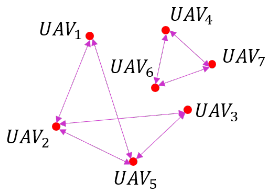
4.4. SL-CBS+ID

After detecting all conflicts within the UAV swarm, a conflict graph is constructed for the UAVs. As shown in Figure 4, we observe that conflicts between $UA{V}_1$, $UA{V}_2$, $UA{V}_3$, and $UA{V}_5$, as well as those between $UA{V}_4$, $UA{V}_6$, and $UA{V}_7$ can be handled in parallel, thus reducing the iteration numbers of the SL-CBS algorithm. The independence detection (ID) technique addresses this issue by determining that, if the optimal solutions for each group of agents are not in conflict with one another, the groups are considered independent. We integrate the ID concept from [25] into the SL-CBS algorithm as follows: (1) Construct a conflict graph from the trajectory results of the UAV swarm; (2) Group the UAV swarm using depth-first search (DFS); (3) Solve each group in parallel using the SL-CBS algorithm; (4) Check whether there are any conflicts in the trajectory results of the entire UAV swarm. If conflicts exist, return to step (1); otherwise, terminate the algorithm. To prevent ID from entering a loop of iterations, we stipulate that, if the ID iteration exceeds a specified value, all agents are grouped together. Overall, with ID acceleration, the optimality and completeness of the original SL-CBS algorithm are maintained, while enabling parallel computation to enhance performance.

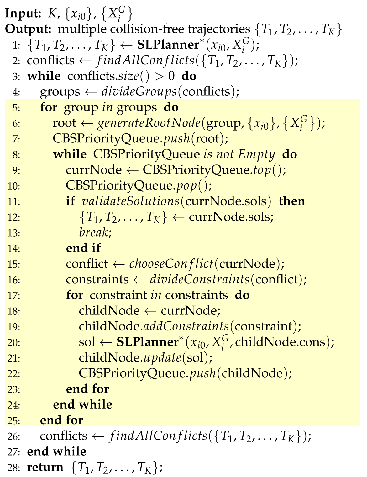
The complete pseudo-code for the SL-CBS+ID algorithm is shown in Algorithm 2. Lines 5–25 outline the SL-CBS algorithm process, while the remaining lines implement the ID. In line 2, a conflict graph is constructed based on the initial solution from line 1. Line 4 involves grouping the UAV swarm based on the conflict graph. Within lines 5–19, line 6 constructs the root node of the $CT$ tree based on the initial states and target regions, where the $CT$ tree is maintained by the priority queue CBSPriorityQueue. In line 9, a greedy search retrieves the current optimal node from the CBSPriorityQueue. Lines 11–14 assess whether the current node has any conflicts; if none are present, the solution is returned. Otherwise, line 15 extracts the earliest occurring conflict for processing. Subsequently, line 16 partitions the relevant constraints for the current conflict. Lines 17–23 handle these constraints, with line 18 constructing new child nodes that inherit the constraints of the parent node. Line 19 adds new constraints, and line 20 resolves the current conflict through replanning based on the improved state lattice. Finally, in line 22, the newly created child nodes are added to the CBSPriorityQueue.

Algorithm 2 SL-CBS+ID

5. Experiment

Our proposed SL-CBS+ID algorithm runs on a system equipped with an Intel Core i7-8700@3.2GHz CPU and 16GB RAM, utilizing Ubuntu and ROS environments. The complete C++ project code is open source at https://github.com/ucas-zihaowang/SL-CBS.git, accessed on 17 November 2024. The complexity of the environment, along with the initial and target states of the UAV swarm and kino-dynamic models, directly affect the results of swarm motion planning. We strictly establish a unified benchmark and consistent UAV kino-dynamic models to ensure the accuracy and fairness of the experimental results. Ultimately, we conduct three types of experiments: classic scenario testing, comparison with baseline algorithms, and analysis of the algorithm’s performance boundaries.

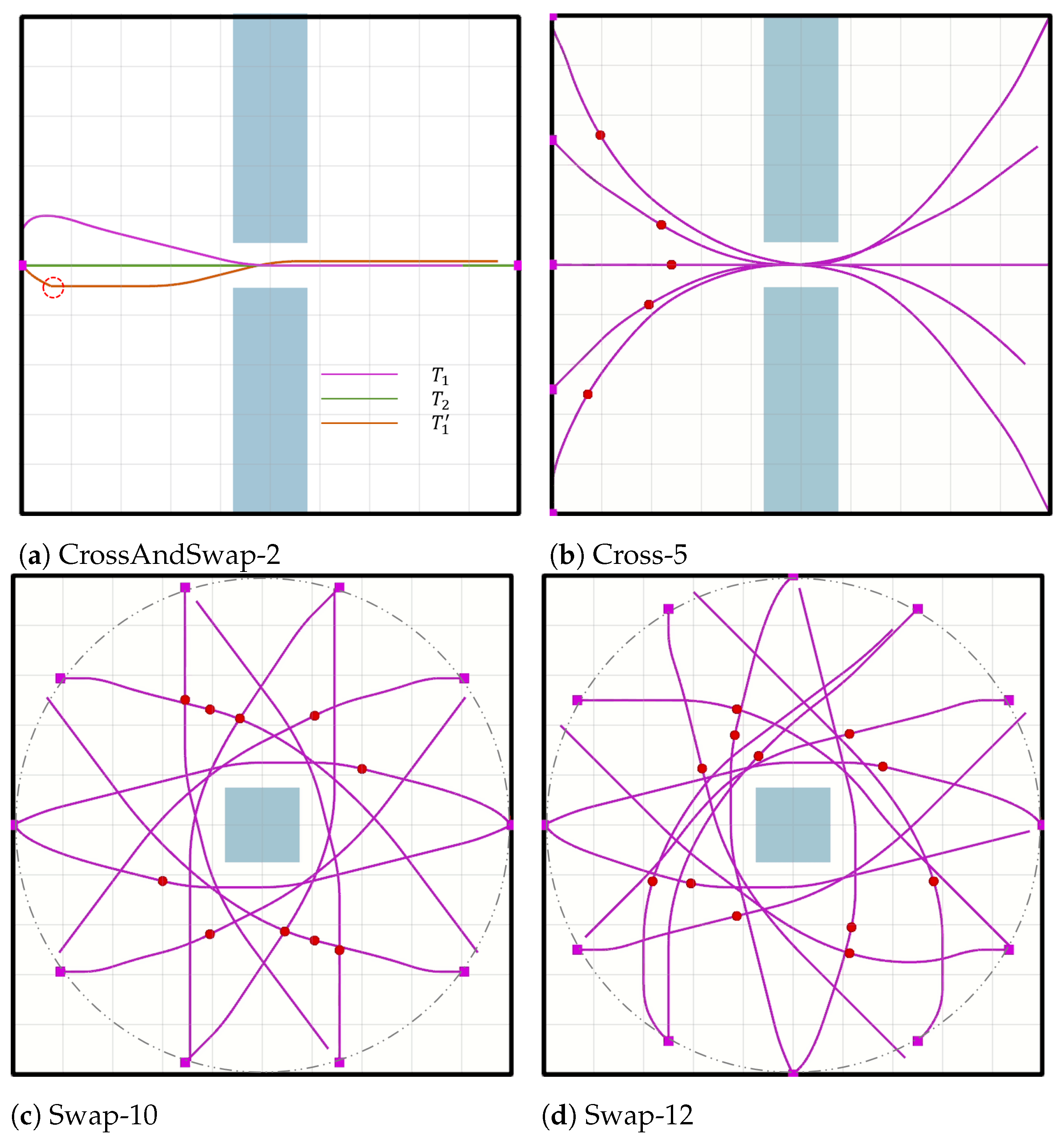
5.1. Test on Classical Scenarios

5.1.1. Setup

The Tunnel Configuration and Star Configuration are two classic test scenarios [2]. Figure 5a,b illustrate the tunnel configuration, while Figure 5c,d show the star configuration, both measuring 10 m by 10 m. The light green rectangular areas represent static obstacles. We conduct three types of tests in these scenarios: CrossAndSwap, Cross, and Swap. The UAV’s maximum speed $v_{max}$ is 2 m/s, with acceleration-based control and a maximum control input $u_{max}$ of 1. The control space sampling number $\mu$ is set to 1, the time interval $\tau$ is 0.5 s, and the time weight of the motion primitive cost function $\rho$ is 10. Additionally, the UAV’s geometric model is a circle with a radius $r_c$ of 0.1 m.

We select sequential planning and decentralized planning from [2] as baseline algorithms. Sequential planning is a centralized algorithm that plans flight trajectories for each UAV in order of priority, treating the trajectories of previously planned UAVs as dynamic obstacles. In decentralized planning, each UAV plans independently, treating others as dynamic obstacles, and iteratively replanning based on a receding horizon control. Both algorithms maintain consistent UAV models and parameters, using computation time, trajectory flight time, and total trajectory cost as evaluation metrics.

5.1.2. Result

In Figure 5a, two UAVs cross a narrow gap to reach each other’s positions, where only one UAV can pass through at a time. $T_1$ is the flight trajectory of $UA{V}_1$ without using an emergency stop, while $T_1^{\prime }$ includes the emergency stop motion primitive, and $T_2$ is the trajectory of $UA{V}_2$. The flight trajectory $T_1^{\prime }$ shows a noticeable emergency stop at the red circle, with a significantly reduced detour. According to

Table 1. Evaluation metrics results of CrossAndSwap-2.

Planner	Cross and Swap-2
	Computation Time	Flight Time	Total Trajectory Cost
SL-CBS (no $p{r}_{stop}$)	706 ms	13.5 s	141
SL-CBS ($p{r}_{stop}$)	1665 ms	13 s	136.5

, using the emergency stop motion primitive reduces both the flight time and total trajectory cost. However, it should be noted that the addition of emergency stop motion primitives increases the search space, leading to a longer computation time. Typically, the increase in computation time is not substantial, but our CrossAndSwap-2 test represents an extreme case.

In Figure 5b–d, we conduct tests for Cross-5 (five UAVs crossing a gap), Swap-10 (10 UAVs swapping positions), and Swap-12 (12 UAVs swapping positions), respectively. According to

Table 2. Evaluation metrics results of classic scenario test instances.

Planner	Cross-5			Swap-10			Swap-12
	Comp. Time	Flight Time	Total Traj. Cost	Comp. Time	Flight Time	Total Traj. Cost	Comp. Time	Flight Time	Total Traj. Cost
Seq Planner [2]	1384 ms	35 s	381	953 ms	58.5 s	628	1304 ms	70 s	758
Dec Planner [2]	4861 ms	43.04 s	465.46	2464 ms	60.45 s	660.65	2684 ms	74.13 s	808.93
SL-CBS	1211 ms	34 s	371.5	2128 ms	58 s	621	27,533 ms	68 s	735
SL-CBS+ID	1220 ms	34 s	371.5	2294 ms	58 s	621	2653 ms	68 s	736

, our proposed SL-CBS shows a great reduction in both trajectory flight time and total trajectory cost across all test instances compared to sequential planning and decentralized planning. This is because sequential planning sacrifices trajectory quality to obtain suboptimal solutions, while decentralized planning focuses on local optima for each UAV, thereby losing the global optimal solution. In terms of computation time, sequential planning is highly efficient as it plans the trajectory for each UAV only once, but it is prone to unsolvable situations in complex environments. Decentralized planning, on the other hand, requires the iterative computation of each UAV’s flight trajectory from its current state to the target region, resulting in a longer computation time. As shown in Table 2, SL-CBS generally takes a longer computation time than sequential planning in most test instances but performs better than decentralized planning. Additionally, we observe that, in the Swap-12 test, due to the dispersed distribution of conflicts, the use of the ID technique greatly reduces the computation time by grouping.

5.2. Compared to Baseline Algorithms

5.2.1. Setup

Most benchmarks for MAPF are based on 4/8-connected grid maps, which cannot be directly applied to continuous space motion planning for UAV swarm. To address this, we design a continuous map with dimensions of 5 m by 5 m, featuring 20 randomly generated circular obstacles with a radius of 0.2 m, resulting in an obstacle density of approximately 10%. The initial and target positions of the UAV swarm must satisfy the following requirements: (1) The initial and target positions of the UAVs must not collide with each other or with the obstacle regions; (2) The Euclidean distance between each UAV’s initial and target position is greater than 1/4 of the map width and less than 3/4 of the map width. Here, the maximum speed of the UAVs $v_{max}$ is 0.5 m/s, with an acceleration-based control and a maximum control input $u_{max}$ of 2, Additionally, the geometric model of the UAVs is a circle with a radius $r_c$ of 0.15 m.

We select the latest algorithms suitable for UAVs, K-CBS [19], and db-CBS [21], which share the same technical approach as SL-CBS, as baseline algorithms. The control interval length is crucial for a fair comparison. K-CBS employs a sampling-based low-level algorithm with control interval lengths varying between $\left[0.1,1\right]$. The db-CBS low-level algorithm is based on db-A*, with pre-computed motion primitives consisting of states and actions at time intervals of 0.1 s. Analysis of db-CBS local motion primitives shows a basic time interval length greater than 0.5 s. Therefore, we set the time interval $\tau$ for SL-CBS to 0.5 s. Given the high obstacle density and complex environment of our benchmark, the SL-CBS control input sampling number $\mu$ is set to 4.

We conduct batch tests with swarm sizes of $K=2,4,6,8,10$, testing each scenario with 10 trials, with a time limit of 300 s. Consistent with the db-CBS project [21], we use the success rate, average computation time, and average trajectory flight time as evaluation metrics.

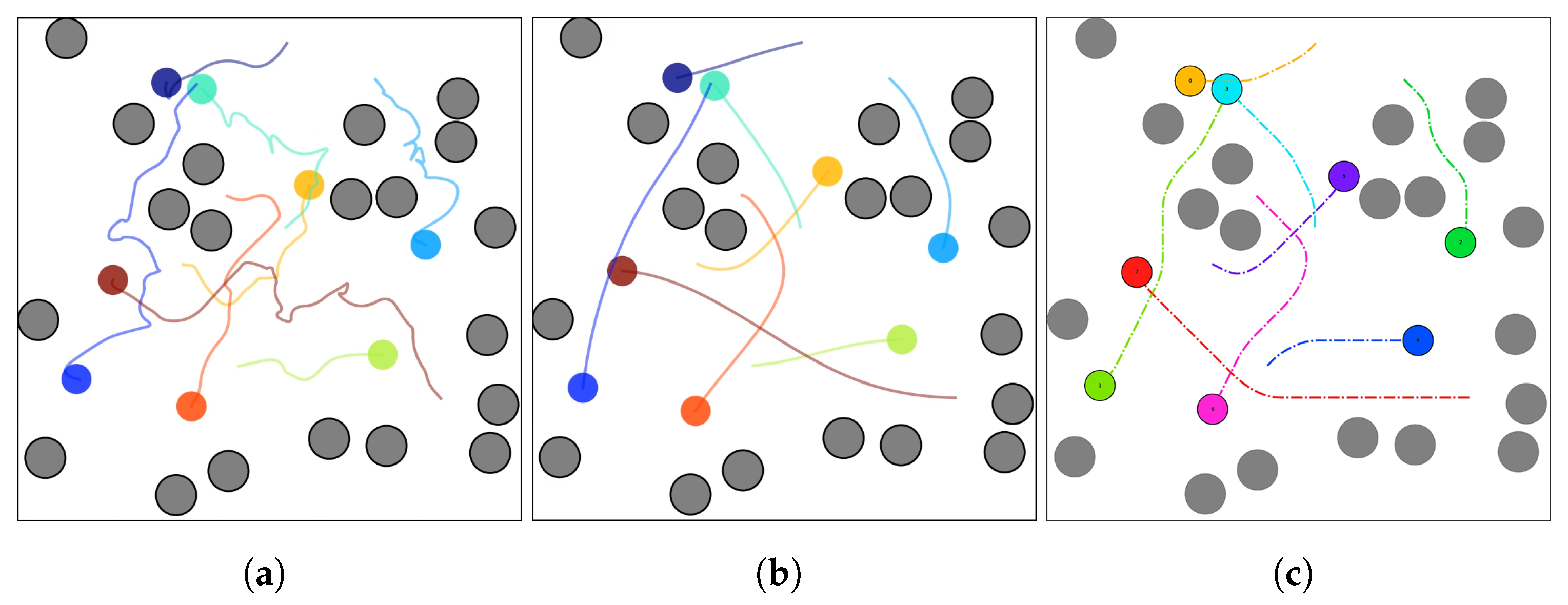
5.2.2. Result

Figure 6 illustrates the flight trajectories of SL-CBS and its baseline algorithms for a swarm size of $K=8$. The trajectories planned by K-CBS are relatively rugged and contain numerous bends, primarily because its low-level search relies on a sampling algorithm and lacks back-end optimization. Although the low-level of db-CBS uses db-A* to search discontinuous trajectories, these become smooth and continuous after trajectory optimization. Our SL-CBS employs an improved state lattice at the low level, which considers complete dynamics, resulting in smooth and continuous trajectories.

Table 3. Evaluation metrics results of K-CBS, db-CBS, and SL-CBS.

Swarm Size	K-CBS			db-CBS			SL-CBS
	Success Rate	Average Comp. Time	Average Flight Time	Success Rate	Average Comp. Time	Average Flight Time	Success Rate	Average Comp. Time	Average Flight Time
$K=2$	1	2.62 s	28.66 s	1	0.38 s	11.61 s	1	0.24 s	9.5 s
$K=4$	1	21.89 s	50.46 s	1	4.77 s	24.89 s	1	0.26 s	20.65 s
$K=6$	0.7	55.3 s	67.66 s	0.9	11.48 s	38.73 s	1	0.62 s	30.6 s
$K=8$	0.5	116.13 s	88.94 s	0.8	36.05 s	53.69 s	1	10.0 2s	41.5 s
$K=10$	0	-	-	0.8	43.91 s	67.93 s	0.9	63.98 s	52.38 s

presents the batch test results for SL-CBS and baseline algorithms across different swarm sizes. Due to the inefficient search of the sampling algorithm and the ineffective conflict interval detection method, K-CBS can only solve most instances for a swarm size of 2–6, consistent with the experimental results in [19]. The db-CBS low-level, utilizing pre-computed motion primitives for search, can solve most instances for a swarm size of 2–10. However, because it includes an additional layer of trajectory optimization and its conflict detection method in the high level is less effective than that of SL-CBS, its computation time is generally longer than SL-CBS. Only for a swarm size of 10 does SL-CBS take a longer time to compute than db-CBS, as our method for calculating an average computation time includes all successfully solved instances. SL-CBS, with its optimal two-layer search, substantially outperforms K-CBS and db-CBS in terms of trajectory flight time. Therefore, based on the test results and the above analysis, SL-CBS demonstrates clear improvements over K-CBS and db-CBS in success rate, computation time, and flight time.

5.3. Performance Boundaries

5.3.1. Setup

Similarly to CL-CBS [17] used in the car-like robots, we conduct batch testing on SL-CBS to analyze its performance boundaries across different swarm sizes. Here, the map size is 50 m by 50 m, with 25 randomly generated circular obstacles, each with a radius of 0.5 m. The initial and target positions of the swarm are randomly generated, consistent with the requirements in Section 5.2. The maximum speed of the UAVs is 2 m/s, controlled by acceleration, with a maximum control input $u_{max}$ of 1. Additionally, we introduce yaw control to achieve full state-space planning for the UAVs, with a maximum yaw of 0.27 radian and a maximum yaw control input of 0.5. We also set the control space sampling number $\mu$ to 1 and the time interval $\tau$ to 1. The geometric model of the UAV is a circle with a radius $r_c$ of 1 m.

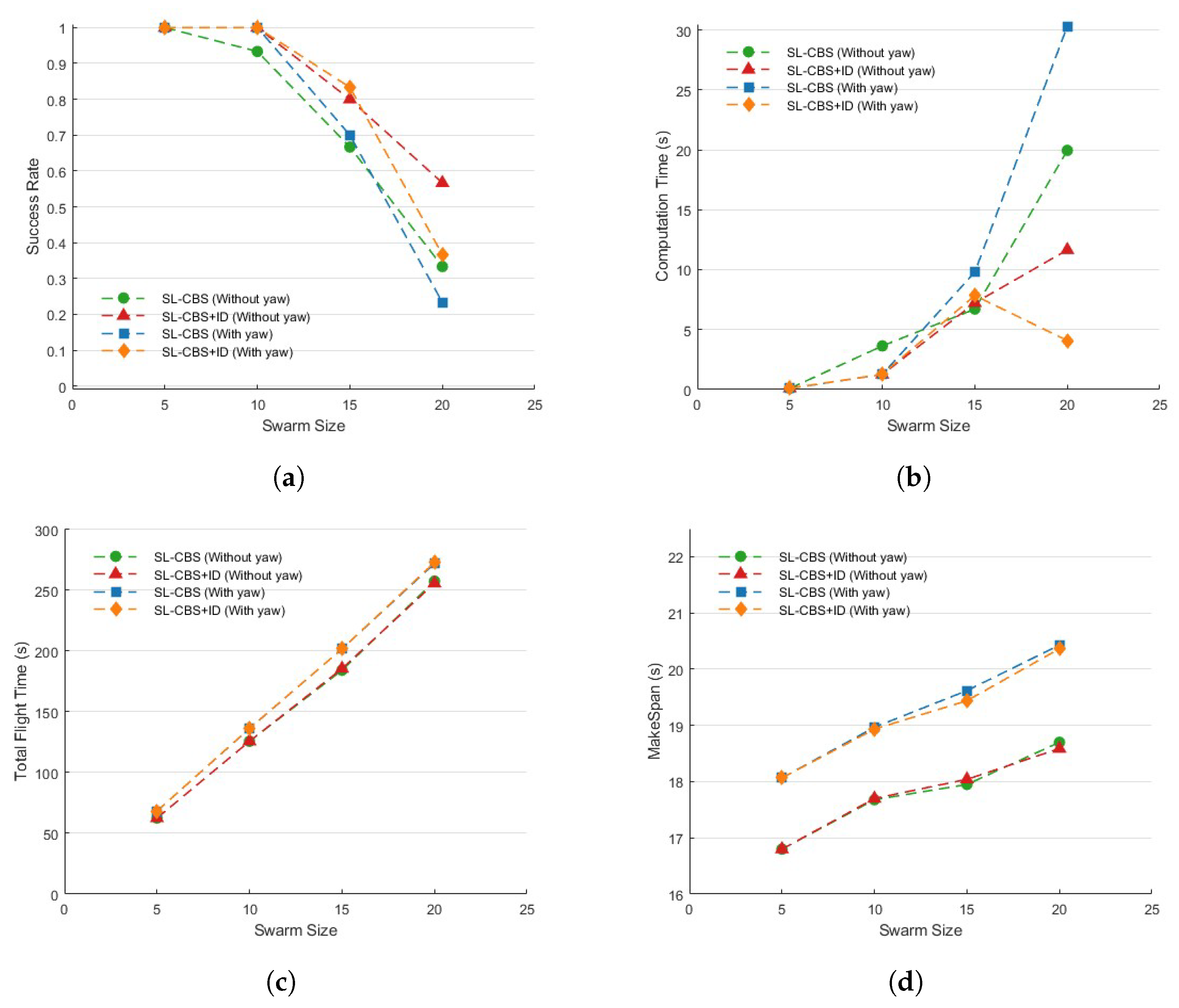
For each randomly generated scenario, we test it with 30 trials, with the computation time limited to 90 s. We conduct batch tests using four algorithm configurations: SL-CBS (Without yaw), SL-CBS+ID (without yaw), SL-CBS (with yaw), and SL-CBS+ID (with yaw), across swarm sizes of 5, 10, 15, and 20. The evaluation metrics are success rate, average computation time, average total trajectory flight time, and average makespan, where makespan is defined as the maximum flight time within the UAV swarm.

5.3.2. Result

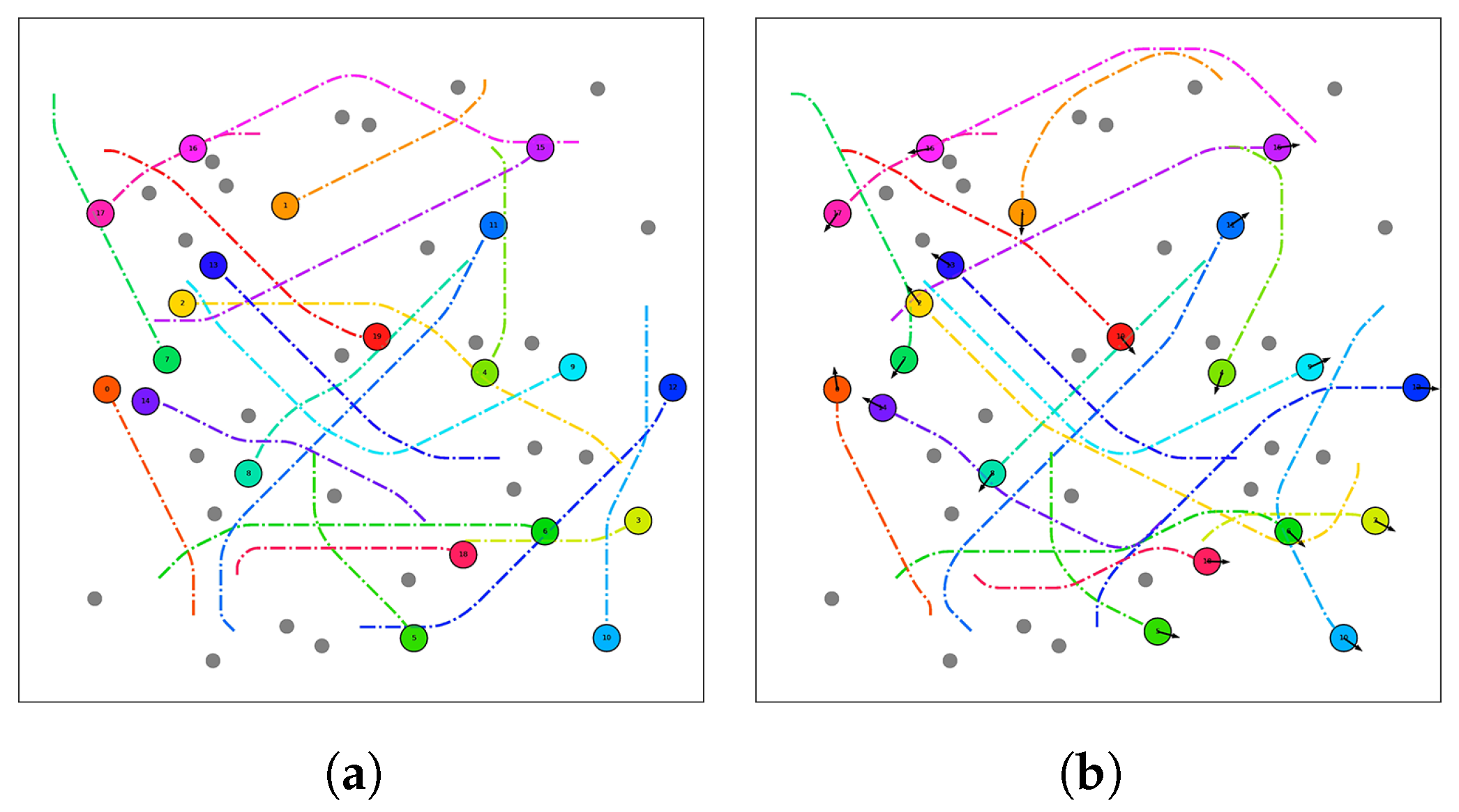
Figure 7 shows the planned trajectories for SL-CBS with and without yaw for a swarm size of 20. It demonstrates the algorithm’s planning capability to solve large-scale, collision-free trajectories in dense environments. Figure 8 illustrates the relationship and trends between various evaluation metrics and swarm size. According to Figure 8a, when the swarm size is 10 or less, SL-CBS+ID can solve all instances, while SL-CBS solves over 90% of them. As the swarm size exceeds 10, the performance of SL-CBS declines, which aligns with the trend in Figure 8b where the computation time increases linearly with swarm size. When the swarm size is 20, SL-CBS+ID (without yaw) still maintains a success rate of over 50%. From Figure 8b, SL-CBS can solve problems within 5 s for swarm sizes of 10 or less, and requires 10 s for a swarm size of 15. It is noteworthy that, for SL-CBS+ID (with yaw), the computation time decreases at a swarm size of 20 due to its lower success rate, which only includes a limited sample of successful instances.

Figure 8c,d reveal that the total trajectory flight time and makespan cost curves for SL-CBS and SL-CBS+ID nearly overlap, further indicating that our ID technique does not affect actual trajectory results. Combined with Figure 8a,b, SL-CBS+ID consistently outperforms SL-CBS. Particularly for a larger swarm size, when the swarm size is 20, the success rate improves by approximately 13.4%, and the computation time is reduced by about 8.3 s.

6. Conclusions

We extend conflict-based search from the MAPF domain to UAV swarm motion planning, formally defining the swarm motion planning problem and proposing the optimal and efficient SL-CBS+ID algorithm. SL-CBS+ID eliminates the need for motion constraints and physical assumptions, making it fully suitable for autonomous UAV swarm flight.

SL-CBS+ID features a two-layer search algorithm: the low-level uses an improved state lattice algorithm for UAVs, incorporating emergency stop primitives and effectively handling spatio-temporal constraints. The high level considers complete state and motion primitive conflicts, introducing a linear time complexity motion conflict detection method based on Sturm’s theory. Additionally, our modified ID is applied to enable parallel conflict processing.

We conduct tests on classic scenarios such as swap and cross. SL-CBS+ID demonstrates substantial advantages over sequential and decentralized planning in terms of flight time and total trajectory cost. It also shows a better computation time in dense environments compared to decentralized planning. By comparing our algorithm within a unified benchmark against the latest SOTA algorithms, K-CBS and db-CBS, our proposed SL-CBS offers clear advantages in success rate, computation time, and trajectory flight time. Finally, we perform the batch testing of SL-CBS+ID to analyze performance boundaries across different swarm sizes.

However, the capability of SL-CBS to solve larger-scale swarm flight trajectories still requires further enhancement. In the future, we plan to explore the application of various CBS improvement techniques, such as conflict classification and high-level heuristic, to SL-CBS. This will aim to enhance its solving capacity without compromising its optimality and completeness. Additionally, SL-CBS currently operates as a one-shot swarm planner, whereas many applications demand lifelong swarm planning. This will also be a focus of our future research.

References

- Chen, J.; Li, J.; Fan, C.; Williams, B.C. Scalable and safe multi-agent motion planning with nonlinear dynamics and bounded disturbances. In Proceedings of the AAAI Conference on Artificial Intelligence, Online, 9 February 2021; Volume 35, pp. 11237–11245. [Google Scholar]
- Liu, S.; Mohta, K.; Atanasov, N.; Kumar, V. Towards search-based motion planning for micro aerial vehicles. arXiv 2018, arXiv:1810.03071. [Google Scholar]
- Li, J.; Ran, M.; Xie, L. Efficient Trajectory Planning for Multiple Non-holonomic Mobile Robots via Prioritized Trajectory Optimization. IEEE Robot. Autom. Lett. 2021, 6, 405–412. [Google Scholar] [CrossRef]
- Yu, J.; LaValle, S. Structure and intractability of optimal multi-robot path planning on graphs. In Proceedings of the AAAI Conference on Artificial Intelligence, Bellevue, WA, USA, 14–18 July 2013; Volume 27, pp. 1443–1449. [Google Scholar]
- Ma, H.; Koenig, S.; Ayanian, N.; Cohen, L.; Hönig, W.; Kumar, T.; Uras, T.; Xu, H.; Tovey, C.; Sharon, G. Overview: Generalizations of multi-agent path finding to real-world scenarios. arXiv 2017, arXiv:1702.05515. [Google Scholar]
- Sharon, G.; Stern, R.; Felner, A.; Sturtevant, N.R. Conflict-based search for optimal multi-agent pathfinding. Artif. Intell. 2015, 219, 40–66. [Google Scholar] [CrossRef]
- Stern, R.; Sturtevant, N.; Felner, A.; Koenig, S.; Ma, H.; Walker, T.; Li, J.; Atzmon, D.; Cohen, L.; Kumar, T.; et al. Multi-agent pathfinding: Definitions, variants, and benchmarks. In Proceedings of the International Symposium on Combinatorial Search, Napa, CA, USA, 16–17 July 2019; Volume 10, pp. 151–158. [Google Scholar]
- Felner, A.; Stern, R.; Shimony, S.; Boyarski, E.; Goldenberg, M.; Sharon, G.; Sturtevant, N.; Wagner, G.; Surynek, P. Search-based optimal solvers for the multi-agent pathfinding problem: Summary and challenges. In Proceedings of the International Symposium on Combinatorial Search, Pittsburgh, PA, USA, 16–17 June 2017; Volume 8, pp. 29–37. [Google Scholar]
- Boyarski, E.; Felner, A.; Stern, R.; Sharon, G.; Betzalel, O.; Tolpin, D.; Shimony, E. Icbs: The improved conflict-based search algorithm for multi-agent pathfinding. In Proceedings of the International Symposium on Combinatorial Search, Ein Gedi, Israel, 11–13 June 2015; Volume 6, pp. 223–225. [Google Scholar]
- Boyarski, E.; Felner, A.; Sharon, G.; Stern, R. Do not split, try to work it out: Bypassing conflicts in multi-agent pathfinding. In Proceedings of the International Conference on Automated Planning and Scheduling, Jerusalem, Israel, 7–11 June 2015; Volume 25, pp. 47–51. [Google Scholar]
- Li, J.; Harabor, D.; Stuckey, P.J.; Ma, H.; Koenig, S. Symmetry-breaking constraints for grid-based multi-agent path finding. In Proceedings of the AAAI Conference on Artificial Intelligence, Honolulu, HI, USA, 27 January–1 February 2019; Volume 33, pp. 6087–6095. [Google Scholar]
- Li, J.; Felner, A.; Boyarski, E.; Ma, H.; Koenig, S. Improved Heuristics for Multi-Agent Path Finding with Conflict-Based Search. In Proceedings of the IJCAI, Macao, China, 10–16 August 2019; Volume 2019, pp. 442–449. [Google Scholar]
- Andreychuk, A.; Yakovlev, K.; Surynek, P.; Atzmon, D.; Stern, R. Multi-agent pathfinding with continuous time. Artif. Intell. 2022, 305, 103662. [Google Scholar] [CrossRef]
- Andreychuk, A.; Yakovlev, K.; Boyarski, E.; Stern, R. Improving continuous-time conflict based search. In Proceedings of the AAAI Conference on Artificial Intelligence, Virtual, 2–9 February 2021; Volume 35, pp. 11220–11227. [Google Scholar]
- Park, C.; Lee, S.; Yang, H.; Shin, D.; Kang, S.; Kim, Y. Conflict-Based Search with Partitioned Groups of Agents for Real-World Scenarios. In Proceedings of the 2023 20th International Conference on Ubiquitous Robots (UR), Honolulu, HI, USA, 25–28 June 2023; pp. 986–992. [Google Scholar]
- Solis, I.; Motes, J.; Sandström, R.; Amato, N.M. Representation-optimal multi-robot motion planning using conflict-based search. IEEE Robot. Autom. Lett. 2021, 6, 4608–4615. [Google Scholar] [CrossRef]
- Wen, L.; Liu, Y.; Li, H. CL-MAPF: Multi-agent path finding for car-like robots with kinematic and spatiotemporal constraints. Robot. Auton. Syst. 2022, 150, 103997. [Google Scholar] [CrossRef]
- Liu, W.; Wang, J.; Zhang, K.; Yu, H.; Zheng, Z.; Lu, G. HG-CBS Planner: Heuristic Group-based Motion Planning for Multi-robot. In Proceedings of the 2023 IEEE 18th Conference on Industrial Electronics and Applications (ICIEA), Ningbo, China, 18–22 August 2023; pp. 687–692. [Google Scholar]
- Kottinger, J.; Almagor, S.; Lahijanian, M. Conflict-based search for multi-robot motion planning with kinodynamic constraints. In Proceedings of the 2022 IEEE/RSJ International Conference on Intelligent Robots and Systems (IROS), Kyoto, Japan, 23–27 October 2022; pp. 13494–13499. [Google Scholar]
- Tajbakhsh, A.; Biegler, L.T.; Johnson, A.M. Conflict-based model predictive control for scalable multi-robot motion planning. In Proceedings of the 2024 IEEE International Conference on Robotics and Automation (ICRA), Yokohama, Japan, 13–17 May 2024; pp. 14562–14568. [Google Scholar]
- Moldagalieva, A.; Ortiz-Haro, J.; Toussaint, M.; Hönig, W. db-cbs: Discontinuity-bounded conflict-based search for multi-robot kinodynamic motion planning. In Proceedings of the 2024 IEEE International Conference on Robotics and Automation (ICRA), Yokohama, Japan, 13–17 May 2024; pp. 14569–14575. [Google Scholar]
- Hönig, W.; Ortiz-Haro, J.; Toussaint, M. db-A*: Discontinuity-bounded Search for Kinodynamic Mobile Robot Motion Planning. In Proceedings of the 2022 IEEE/RSJ International Conference on Intelligent Robots and Systems (IROS), Kyoto, Japan, 23–27 October 2022; pp. 13540–13547. [Google Scholar]
- Liu, S.; Atanasov, N.; Mohta, K.; Kumar, V. Search-based motion planning for quadrotors using linear quadratic minimum time control. In Proceedings of the 2017 IEEE/RSJ International Conference on Intelligent Robots and Systems (IROS), Vancouver, BC, Canada, 24–28 September 2017; pp. 2872–2879. [Google Scholar]
- Wang, Z.; Zhou, X.; Xu, C.; Chu, J.; Gao, F. Alternating minimization based trajectory generation for quadrotor aggressive flight. IEEE Robot. Autom. Lett. 2020, 5, 4836–4843. [Google Scholar] [CrossRef]
- Standley, T. Finding optimal solutions to cooperative pathfinding problems. In Proceedings of the AAAI Conference on Artificial Intelligence, Atlanta, GA, USA, 11–15 July 2010; Volume 24, pp. 173–178. [Google Scholar]
Figure 1.
Planning process of the SL-CBS algorithm. The black border represents the map boundary, the light green rectangles denote static obstacles, the blue hollow circles indicate the initial positions of the UAVs, and the cyan hollow circles represent the UAVs’ target regions. The magenta curves depict the planned UAV flight trajectories, with the solid red circles on the curves indicating the UAV states. (a) initial state; (b) the first iteration; and (c) the second iteration.
Figure 2.
Two types of conflicts. In (a), a state conflict occurs at the extended state at time , while in (b), a motion primitive conflict occurs at some location within . Here, is time interval.
Figure 3.
Emergency stop motion primitive model.
Figure 4.
UAV swarm conflict graph. The magenta double-headed arrows represent the existence of conflicts between the trajectories of the UAVs.
Figure 5.
Flight trajectories of UAV swarm in classic scenario test instances. The black border represents the map boundary, while the light green areas indicate static obstacles. The magenta curves depict the flight trajectories of the UAVs. In (a), the green and orange curves also represent UAV flight trajectories. In (b–d), the solid red circles indicate the flight states of the UAV at intermediate times.
Figure 6.
Flight trajectories planned by K-CBS, db-CBS, and SL-CBS for swarm size . The black border represents the map boundaries, while the 20 gray circles indicate obstacle regions. The solid circles in various colors depict the current states of the UAV swarm, and the curves in different colors represent the trajectories already flown by the UAV swarm. (a) K-CBS; (b) db-CBS; and (c) SL-CBS.
Figure 7.
Flight trajectories planned by SL-CBS for a swarm size of . The black border represents the map boundary, while the 25 gray circles indicate obstacle regions. The solid circles in various colors represent the current states of the UAV swarm, with black arrows on the circles indicating the yaw direction of each UAV. The curves in different colors illustrate the trajectories already traveled by the UAV swarm. (a) (without yaw); and (b) (with yaw).
Figure 8.
Evaluation metrics results of SL-CBS under different swarm sizes: (a) success rate; (b) computation time; (c) total flight time; and (d) makespan.