A Vision-Based End-to-End Reinforcement Learning Framework for Drone Target Tracking

Abstract

Drone target tracking, which involves instructing drone movement to follow a moving target, encounters several challenges: (1) traditional methods need accurate state estimation of both the drone and target; (2) conventional Proportional–Derivative (PD) controllers require tedious parameter tuning and struggle with nonlinear properties; and (3) reinforcement learning methods, though promising, rely on the drone’s self-state estimation, adding complexity and computational load and reducing reliability. To address these challenges, this study proposes an innovative model-free end-to-end reinforcement learning framework, the VTD3 (Vision-Based Twin Delayed Deep Deterministic Policy Gradient), for drone target tracking tasks. This framework focuses on controlling the drone to follow a moving target while maintaining a specific distance. VTD3 is a pure vision-based tracking algorithm which integrates the YOLOv8 detector, the BoT-SORT tracking algorithm, and the Twin Delayed Deep Deterministic Policy Gradient (TD3) algorithm. It diminishes reliance on GPS and other sensors while simultaneously enhancing the tracking capability for complex target motion trajectories. In a simulated environment, we assess the tracking performance of VTD3 across four complex target motion trajectories (triangular, square, sawtooth, and square wave, including scenarios with occlusions). The experimental results indicate that our proposed VTD3 reinforcement learning algorithm substantially outperforms conventional PD controllers in drone target tracking applications. Across various target trajectories, the VTD3 algorithm demonstrates a significant reduction in average tracking errors along the X-axis and Y-axis of up to $34.35\%$ and $45.36\%$, respectively. Additionally, it achieves a notable improvement of up to $66.10\%$ in altitude control precision. In terms of motion smoothness, the VTD3 algorithm markedly enhances performance metrics, with improvements of up to $37.70\%$ in jitter and $60.64\%$ in Jerk RMS. Empirical results verify the superiority and feasibility of our proposed VTD3 framework for drone target tracking.

1. Introduction

Autonomous drone control technology has been extensively adopted in sectors such as agriculture [1], military operations [2], and search-and-rescue missions [3], thereby enhancing task efficiency, reducing operational costs, and mitigating human risk. Drones can also optimize mining operations by conducting terrain surveys, monitoring safety conditions, and collecting data [4]. Additionally, they are capable of accessing environments that are typically inaccessible or pose high risks, such as areas with nuclear contamination [5] or chemical spill sites [6].

In the domain of autonomous drone target tracking, conventional methods predominantly depend on accurate coordinate relationships between the drone and the target to devise tracking strategies [7]. Nevertheless, drones frequently operate in intricate environments where they may encounter GPS signal loss and imprecise self-state estimation [8], potentially resulting in the failure of traditional tracking strategies. Vision-based tracking methods utilizing monocular cameras present a viable alternative. Recent studies [9] have introduced innovative methodologies that leverage the bounding box area generated by object detection algorithms as a proxy for distance estimation, thereby effectively mitigating the depth estimation issue.

Upon acquiring target information through object detection algorithms, it is imperative for controllers to generate control commands for the drone. Scholars commonly categorize controllers into two distinct components: high-level controllers, which are tasked with determining the drone’s desired position, velocity, and navigation parameters [10,11,12], and low-level controllers, which are responsible for managing the drone’s attitude to effectively implement the directives issued by the high-level controllers. Although optimal solutions for low-level controllers have been extensively studied [13], high-level controllers still face challenges. Among model-based methods, Model Predictive Control (MPC) [14] utilizes system models to predict future states and optimize control actions. However, when faced with highly nonlinear tasks, its performance heavily relies on model accuracy and incurs high computational costs [15]. The Probabilistic Ensembles with Trajectory Sampling (PETS) [16] method enhances robustness by combining ensemble dynamics models with sampling-based uncertainty propagation, but it demonstrates instability in highly nonlinear and uncertain tasks [17]. Model-Based Policy Optimization (MBPO) [18] enhances sample efficiency by integrating model-based planning with policy optimization; however, due to the inevitable errors in learned models, it struggles to achieve the same asymptotic performance as model-free methods [19]. In the realm of model-free methods, Proximal Policy Optimization (PPO) [20], a policy gradient approach, improves the stability of policy updates. However, as an on-policy algorithm, PPO suffers from sample inefficiency and poor policy exploration [21]. The Deep Deterministic Policy Gradient (DDPG) [22] integrates deep neural networks with deterministic actor–critic methods, demonstrating effective learning in continuous action spaces. Nevertheless, the DDPG was found to be sensitive to hyperparameters and exhibited stability issues.

To address these limitations, the Twin Delayed Deep Deterministic Policy Gradient (TD3) algorithm [23] was developed. As an enhancement of the DDPG, the TD3 incorporates novel mechanisms such as a delayed training architecture and clipped double Q-learning [24]. These innovations significantly improve the algorithm’s stability and performance by addressing overestimation bias. The TD3 excels in handling nonlinear dynamics and offers high learning efficiency, making it a strong baseline for continuous control tasks, particularly in complex environments such as drone target tracking.

This paper aims to investigate a novel vision-based reinforcement learning tracking system named VTD3 to enhance the accuracy and stability of drone target tracking. The VTD3 system integrates computer vision and reinforcement learning techniques, establishing an efficient closed-loop control architecture. It employs YOLOv8 [25] for real-time object detection and incorporates the BoT-SORT [26] algorithm to achieve precise target tracking. Detection results are transformed into state vectors and input into the TD3 network to generate corresponding control actions. The system continuously optimizes network performance through reward calculation and executes final control commands via a low-level control module. This closed-loop design enables VTD3 to continuously learn and adapt to changing environments, progressively enhancing the effectiveness and robustness of its control strategies.

The main contributions of this work are as follows:

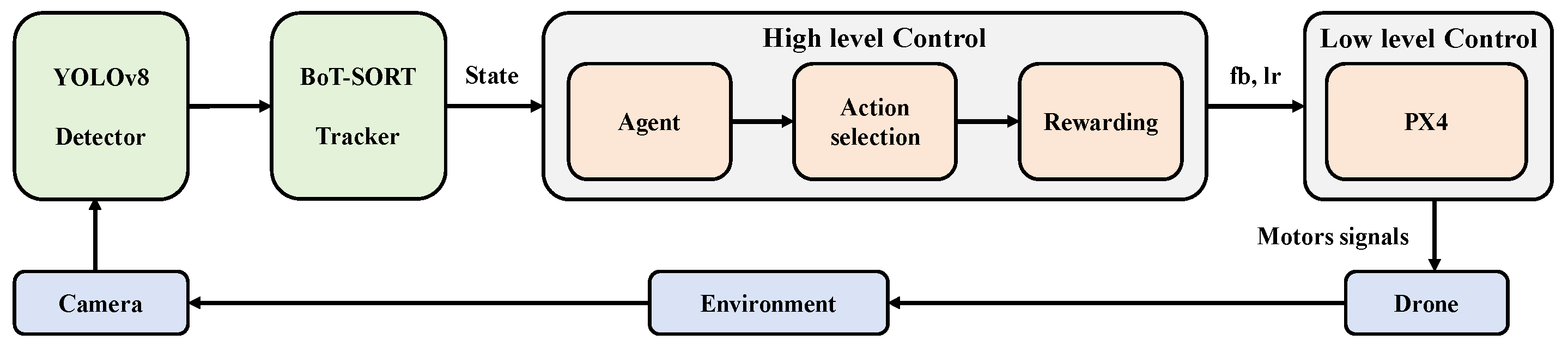
• We propose an advanced end-to-end reinforcement learning framework named VTD3, specifically designed for drone target tracking. This framework synergistically incorporates the YOLOv8 detection model, the BoT-SORT tracking algorithm, and the TD3 algorithm. Through this integration, the TD3 algorithm is trained to function as the drone’s high-level controller, thereby facilitating efficient and autonomous target tracking.
• We introduce a vision-based navigation strategy that significantly reduces reliance on GPS and ancillary sensors. This advancement enhances the system’s adaptability and reliability in complex environments while reducing hardware demands and overall system complexity.
• We showcase the tracking performance of our proposed VTD3, which significantly enhances the system’s handling of nonlinear and highly dynamic target motions. Experiments reveal notable gains for VTD3 in tracking accuracy, jitter reduction, and motion smoothness over traditional PD controllers.

The subsequent sections of this paper are organized as follows: Section 2 reviews related work. Section 3 elaborates on the methodology, including the algorithms employed and the simulation software. Section 4 presents the experimental design and analyzes the results. Finally, Section 5 concludes the study and explores potential directions for future research.

2. Related Works

This section provides a comprehensive overview of recent advancements in drone target tracking and the application of reinforcement learning for drone control. The intersection of these domains forms a critical foundation for our research.

2.1. Drone Target Tracking

In recent years, there have been notable advancements in drone target tracking technology. Sun et al. [27] conducted an extensive review of the field, proposing a novel classification framework that categorizes target tracking techniques into detection tracking, following tracking, and cooperative tracking. Detection tracking focuses on target appearance changes, often using correlation filters or deep learning, while following tracking emphasizes controlling UAV flight based on target movement. Cooperative tracking involves multiple UAVs working together, such as swarms using reinforcement learning.

Ajmera and Singh [28] developed an advanced system for autonomous UAV-based search and rescue. Their approach combines reinforcement learning for navigation, YOLO for target detection, and optical flow for tracking. The system enables drones to efficiently locate victims in unknown environments, then track and follow them in real time. Simulations demonstrated its effectiveness in realistic urban search-and-rescue scenarios. Liu et al. [29] introduced an end-to-end visual navigation system leveraging deep learning techniques. They optimized YOLOX for runway region-of-interest detection and designed RLDNet for precise runway line detection. The system further employs Kalman filtering to fuse visual localization results with IMU data, enhancing positioning accuracy. Simulations and flight tests demonstrated the system’s superior detection accuracy, real-time performance, and generalization capability in various scenarios.

Sun et al. [9] introduced a real-time target tracking system utilizing Siamese Transformer networks (SiamTrans), effectively addressing the trade-off between speed and accuracy in visual tracking systems. Using the UAV123 benchmark, SiamTrans improves the success rate by 3.6% compared to SiamRPN++ while maintaining comparable speed on the NVIDIA Jetson AGX Xavier embedded platform. The authors also proposed a Tracking Drift Suppression Strategy to enhance robustness in complex scenes. Farkhodov et al. [30] implemented an integration of deep reinforcement learning (DRL) with the AirSim virtual simulation platform to advance drone tracking capabilities in complex environments. By employing a DQN and RNN for prediction and control tasks, their method exhibited superior performance on the VisDrone2019 and OTB-100 datasets. Compared to the ADNet approach, their method improved accuracy by 11.07% on the OTB-100 dataset. On the VisDrone2019 dataset, it outperformed ASRL Track by 7.35%.

2.2. Drone Reinforcement Learning

In recent years, significant advancements have been made in the application of reinforcement learning within the domain of unmanned aerial vehicles (UAVs). Liu and Suzuki [13] introduced a novel approach that integrates a Proportional–Integral–Derivative (PID) low-level controller with a Proximal Policy Optimization (PPO) algorithm to enhance high-level navigation planning. This deep-reinforcement-learning-based method demonstrated the capability to achieve high-speed and safe navigation in complex environments, attaining a maximum velocity of 7 m per second, thereby more than doubling the performance metrics of conventional PID controllers. Sha and Wang [31] introduced a deep reinforcement learning framework tailored for autonomous navigation in resource-constrained environments. This framework also combines PPO and PID algorithms, integrating PID algorithms to manage drone attitude and position control while employing the PPO algorithm to enhance navigation planning. To adapt to constrained environments, they designed a customized reward function incorporating penalties for obstacles and out-of-bounds movements, as well as rewards for reaching the target position. Their experiments in a simulated Pybullet environment demonstrated the framework’s ability to navigate a quadcopter UAV to a target position while avoiding obstacles within a limited space.

Li et al. [32] proposed a novel approach utilizing an enhanced Deep Deterministic Policy Gradient (MN-DDPG) algorithm combined with transfer learning to facilitate autonomous real-time tracking and obstacle avoidance for maneuvering targets. This methodology integrates mixed noise to aid in the exploration of random policies and improves generalization capabilities through task decomposition and pre-training. Their experimental results demonstrated that the MN-DDPG with transfer learning approach achieved stable high rewards after only 270 training episodes, significantly outperforming the traditional DDPG, which required about 480 episodes to show unstable improvements. Srivastava et al. [33] introduced a method for maneuvering target tracking that employs least squares policy iteration (LSPI) and relies exclusively on visual feedback. This approach learns optimal control policies through interaction with the environment, thereby eliminating the need for predefined interaction matrices. In planar target tracking scenarios, their LSPI-based controller achieved relatively small root mean square errors along all three axes, outperforming conventional methods. The approach demonstrated robust performance in both 2D and 3D tracking tasks.

Ma et al. [34] and Mosali et al. [35] investigated the application of reinforcement learning in the domains of drone camera gimbal control and target tracking, respectively. Ma et al. applied the DDPG to camera gimbal control, achieving a stable reward convergence and reducing unnecessary movements to a two-step tracking process. Their approach demonstrated superior performance in continuous and mixed interference environments compared to PID control. Mosali et al. combined the TD3 with a PD controller for exploration enhancement, and introduced a novel reward formulation incorporating exponential functions to limit velocity and acceleration effects. Their method achieved an up to 86% error reduction compared to traditional controllers in tracking fixed, moving, and blinking targets.

For the autonomous landing task, Vankadari et al. [36] proposed a least squares policy iteration (LSPI) reinforcement learning method to achieve precise quadrotor drone landings. This method was trained in simulation and deployed on a real drone equipped with PTAM visual odometry and demonstrated effective landing trajectory generation and accurate landings within 20 cm of the target in complex real-world environments while showing robustness to sensor noise and temporary marker loss. In the domain of multi-agent collaboration, Du et al. [37] proposed a cellular-enabled MARL framework for the cooperative pursuit of unauthorized drones in urban airspace, integrating parameter sharing and curriculum learning to significantly improve capture performance. Their experimental results demonstrated that the proposed method achieved an 81.1% capture probability and an average capture time of 29.21 s when pursuing an evader 1.3 times faster than the pursuers, significantly outperforming baseline approaches.

3. Methods

This section presents our proposed reinforcement-learning-based methodology for drone target tracking. Initially, we provide an overview of the framework design, highlighting the integration of computer vision and reinforcement learning techniques. Subsequently, we delve into the essential components of the system: the YOLOv8 detector, the BoT-SORT tracker, and the TD3 controller. Finally, we introduce the SIGMA simulation environment utilized for performance evaluation. Collectively, these methods constitute an efficient solution for drone target tracking.

3.1. Framework

The proposed vision-based end-to-end reinforcement learning framework, denoted as VTD3, is illustrated in Figure 1. VTD3 integrates computer vision and reinforcement learning techniques, enabling seamless transition from visual input to control output. The primary workflow encompasses the following steps: employment of YOLOv8 for object detection and BoT-SORT for target tracking, deriving state vectors from the detection outcomes, utilizing a TD3 network to produce control actions based on these state vectors, calculating reward values for training the network, and ultimately executing control commands via low-level control (PX4 flight control system) to facilitate interaction with the environment. This closed-loop design enables the system to perpetually learn and optimize control strategies. The TD3 algorithm guarantees stability and efficiency throughout the learning process, while advanced computer vision techniques furnish precise environmental perception capabilities.

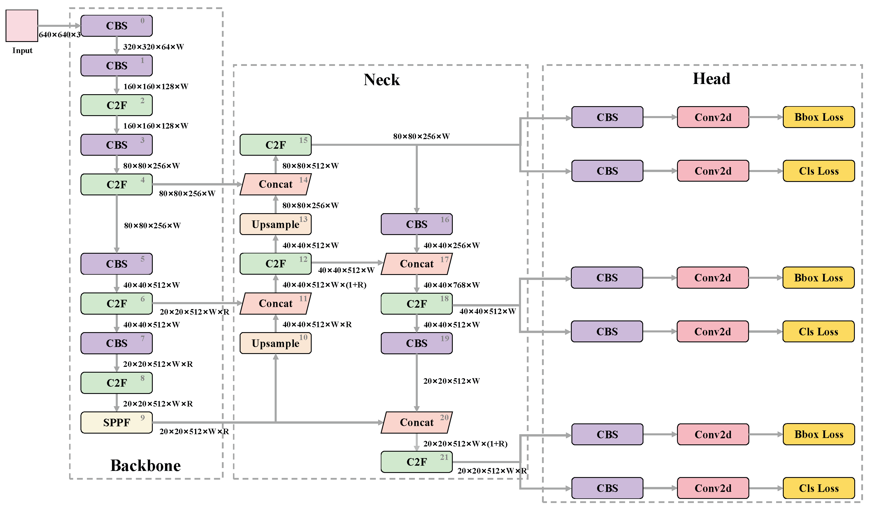
3.2. YOLOv8 Detector

3.2.1. Model Structure

YOLOv8 [25] represents a novel state-of-the-art (SOTA) model for object detection and instance segmentation, available in two resolutions: P5 at 640 pixels and P6 at 1280 pixels. The model adheres to the scaling strategy employed in YOLOv5 [38] and is offered in various versions (N/S/M/L/X) to address diverse application requirements. As illustrated in Figure 2, YOLOv8’s architecture consists of several key components: a backbone for feature extraction, a neck for feature fusion, and a head for final detection and classification.

Key improvements in YOLOv8 include an enhanced backbone architecture for more efficient feature extraction, a refined neck structure for better feature fusion, and an advanced head design for improved detection accuracy. These advancements result in improved overall performance and lower resource consumption compared to previous architectures, making it particularly suitable for real-time applications such as drone-based target tracking. In our study, we utilize YOLOv8 for its superior object detection capabilities, which are crucial for accurate target identification and tracking in drone applications. The model’s efficiency and accuracy contribute significantly to our system’s ability to maintain reliable target tracking while operating under the computational constraints of a drone platform.

3.2.2. Loss Function

The loss function is a metric to quantify the difference between model predictions and ground truth labels, thereby facilitating the optimization of model parameters during the training process. In the context of YOLOv8, the loss function is composed of several components, with the primary elements being classification loss and regression loss.

Classification Loss: YOLOv8 employs Varifocal Loss (VFL) as its classification loss. VFL represents an advancement over binary cross-entropy (BCE) by dynamically adjusting loss weights according to the overlap between predicted and target bounding boxes. This adjustment effectively mitigates the imbalance between positive and negative samples. Let p denote the predicted IACS (Intersection over Area of Circumscribing Square), a metric for assessing prediction accuracy, and q denote the IOU (Intersection over Union), a metric for object detection accuracy between the candidate box and the ground truth box. For negative samples, the value of q is set to 0. $\alpha$ is a scaling factor that controls the overall magnitude of the loss for negative samples, while $\gamma$ is an exponential factor that adjusts the sensitivity of the loss to predictions with different confidence levels. The VFL formula is as follows:

$$\mathrm{VFL}(p,q)=\left\{\begin{array}{cc}-q·[qlog(p)+(1-q)log(1-p\left)\right]\hfill & \mathrm{if}q>0\hfill \\ -\alpha p^{\gamma }log(1-p)\hfill & \mathrm{if}q=0\hfill \end{array}\right.$$

(1)

Regression Loss: The regression loss consists of two parts: CIOU (Complete IoU) Loss and Distribution Focal Loss (DFL).

(a) CIOU Loss: The CIOU Loss extends the traditional IoU Loss by integrating additional metrics such as the distance between center points and the aspect ratio of bounding boxes. This extension offers a more holistic evaluation of the alignment between predicted and target boxes. d is the center point distance, c is the diagonal length of the bounding box, v is the measure of aspect ratio consistency, and $\alpha >0$ is a balance parameter. The formula for CIOU Loss is as follows:

$$L_{CIOU}=1-IoU+{\displaystyle \frac{d^2}{c^2}}+\alpha v$$

(2)

(b) Distribution Focal Loss (DFL): DFL is introduced to support the Anchor-Free paradigm. It improves the model’s generalization ability in complex scenarios by optimizing the probability distribution around the target location. Let ${\mathcal{S}}_i$ and ${\mathcal{S}}_{i+1}$ represent the “predicted value” and the “adjacent predicted value” output by the network, respectively. y denotes the “actual value” of the label, while $y_i$ and $y_{i+1}$ correspond to the “label integral value” and “adjacent label integral value”, respectively. The DFL formula is as follows:

$$\mathrm{DFL}({\mathcal{S}}_i,{\mathcal{S}}_{i+1})=-((y_{i+1}-y)log\left({\mathcal{S}}_i\right)+(y-y_i)log\left({\mathcal{S}}_{i+1}\right))$$

(3)

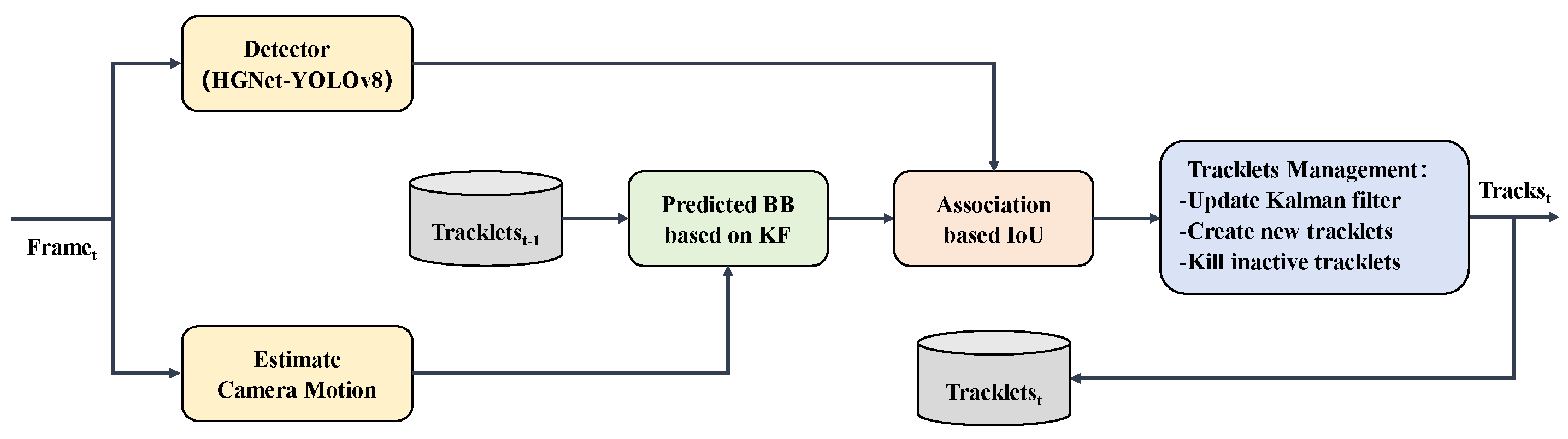
3.3. BoT-SORT Tracker

BoT-SORT [26] is an advanced “Tracking-by-Detection” paradigm engineered to precisely track the spatiotemporal trajectories of multiple objects in video streams. This algorithm finds extensive application in contexts such as autonomous driving and video surveillance. Notably, considering the computational resource constraints and deployment considerations, the implementation of the BoT-SORT in this paper omits the ReID module.

The workflow of BoT-SORT is illustrated in Figure 3. It contains three stages: detection, tracking, and track management. During the detection stage, the YOLOv8 is employed to identify objects within video frames. In the tracking stage, an enhanced Kalman filter is utilized to construct the motion model of the targets, thereby facilitating the prediction of their positions in subsequent frames. Traditionally, most tracking methods, such as those employed in Deep SORT [39], utilize a seven-element state vector (Equation (4)) that includes the bounding box’s center coordinates $(x,y)$, area (s), and aspect ratio (r).

$$x_k={[x_c\left(k\right),y_c\left(k\right),s,r,{\dot{x}}_c\left(k\right),{\dot{y}}_c\left(k\right),\dot{s}]}^T$$

(4)

However, as the aspect ratio alone does not adequately characterize a bounding box (bbox), BoT-SORT refines the state representation to an eight-element vector. This modification involves substituting the area and aspect ratio with the precise values of bbox width (w) and height (h), thereby improving the accuracy of the predicted bbox, as shown in Equation (5).

$$x_k={\left[\begin{array}{c}{x}_c\left(k\right),y_c\left(k\right),w\left(k\right),h\left(k\right),{\dot{x}}_c\left(k\right),{\dot{y}}_c\left(k\right),\dot{w}\left(k\right),\dot{h}\left(k\right)\end{array}\right]}^T$$

(5)

BoT-SORT introduces a tracking methodology based on camera motion compensation. Trackers that utilize the “Tracking-by-Detection” paradigm are heavily dependent on the overlap between the predicted and detected bbox. In scenarios involving dynamic camera settings, substantial displacements in the bbox positions on the image plane can occur, which may result in ID switches or false negatives. BoT-SORT addresses this issue by employing global motion estimation (GMC) techniques from OpenCV to model background motion.

Initially, image keypoints are extracted and tracked using sparse optical flow in conjunction with translation-based local outlier suppression. Subsequently, the Random Sample Consensus (RANSAC) algorithm is employed to compute the affine transformation matrix, facilitating the transition of the predicted bbox from frame $k-1$ to frame k. Following the completion of IoU calculation, the track management module is responsible for updating and maintaining the tracks. This module not only updates the association of new detections with existing tracks but also addresses occlusions and interactions among objects. Additionally, it evaluates the validity of tracks by assessing the continuity and reliability of detections to decide whether to continue or terminate a track. Through meticulous management, BoT-SORT ensures high accuracy and stability, optimizing the overall performance of the tracking system.

3.4. TD3-Based Controller

3.4.1. TD3 Algorithm Architecture

The Twin Delayed Deep Deterministic Policy Gradient (TD3) is a reinforcement learning algorithm specifically designed for continuous action spaces. It effectively mitigates the overestimation bias commonly associated with the DDPG algorithm. The TD3 achieves this by integrating dual Q-learning, delayed policy updates, and target policy smoothing techniques, which collectively enhance the stability and performance of the algorithm. The core architecture of the TD3 consists of two critic networks, referred to as Critic1 and Critic2, alongside an actor network. Furthermore, each of these networks is paired with corresponding target networks, namely, Critic_T1, Critic_T2, and Actor_T, which facilitate the accurate updating of target values during the training process.

The training process of the TD3 is shown in Figure 4. Initially, the actor network and both critic networks, along with their corresponding target counterparts, are initialized. The algorithm then interacts with the environment to collect experiences, which are subsequently stored in a replay buffer. During the training phase, the algorithm draws batches of samples from the replay buffer. The target critic networks, Critic_T1 and Critic_T2, along with the target actor network Actor_T, are used to compute the target values for the subsequent states. In particular, during the parameter update process for the Critic1 and Critic2 networks, the subsequent state action $A^{\prime }$ is first determined using the target actor network Actor_T. Subsequently, the algorithm evaluates $A^{\prime }$ by both target critic networks, Critic_T1 and Critic_T2, with the lesser of the two evaluations being selected. This minimum value, combined with the immediate reward r and the discount factor $\gamma$, constitutes the target value y. The critic networks are then updated by minimizing the mean squared error between their outputs and the calculated target value y. Let $Q{1}^{\prime }$ and $Q{2}^{\prime }$ represent the target critic networks Critic_T1 and Critic_T2, respectively, and $s^{\prime }$ denote the subsequent state. The target value y is then calculated as follows:

$$y=r+\gamma ·min\left(Q{1}^{\prime }(s^{\prime },A^{\prime }\left(s^{\prime }\right)),Q{2}^{\prime }(s^{\prime },A^{\prime }\left(s^{\prime }\right))\right)$$

(6)

To enhance the regulation of policy updates and mitigate variance, the TD3 employs a delayed update mechanism for the actor network. Specifically, the actor network is updated at a lower frequency compared to the critic networks. Additionally, the parameters of all target networks are gradually aligned with their corresponding main networks via a soft update mechanism, thereby ensuring a smooth and stable learning process.

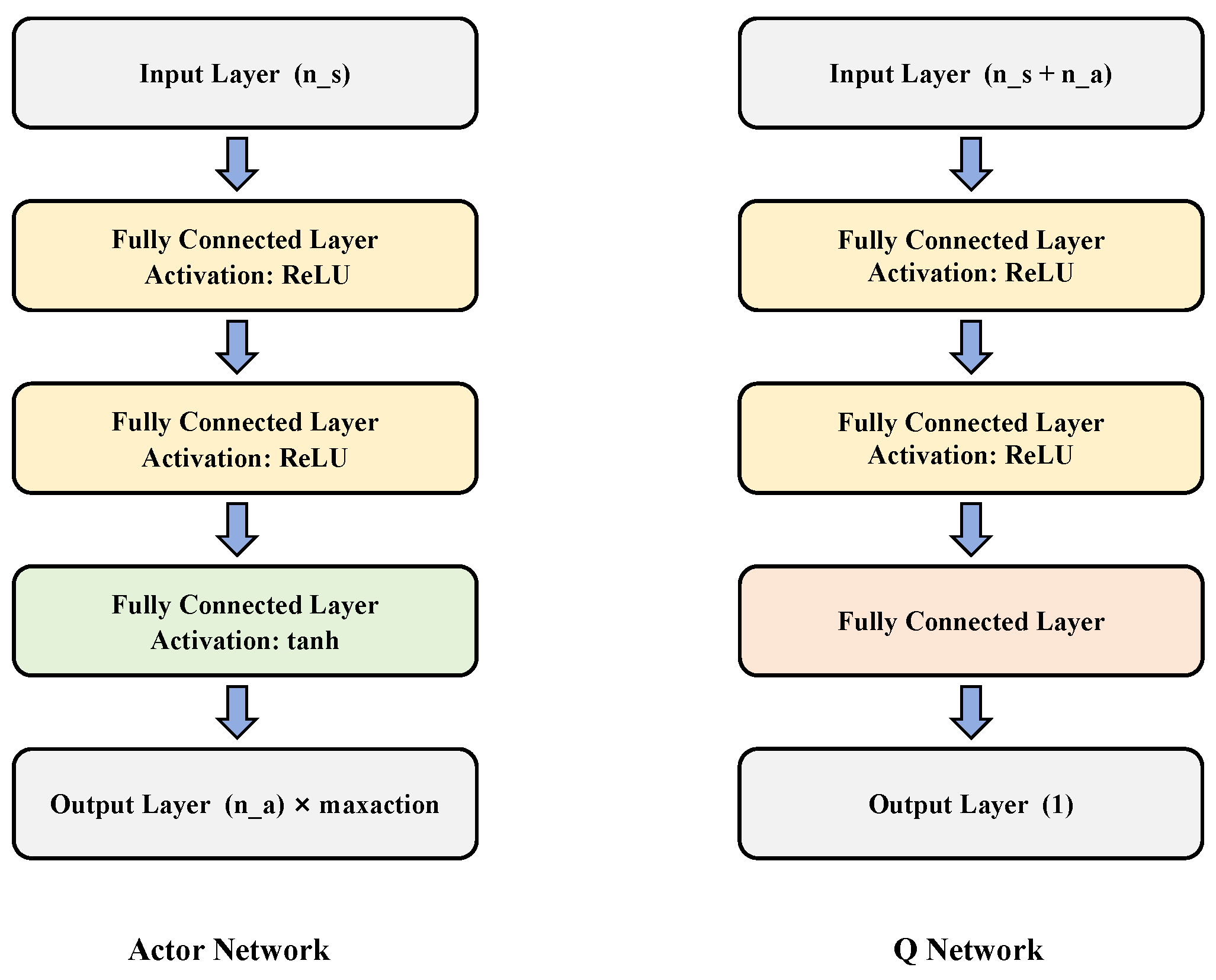
3.4.2. Actor and Q Network Structures

In the TD3, both the actor network and the two Q networks employ fully connected feedforward neural network architectures, as illustrated in Figure 5. The actor network takes a state s with dimension $n\_s$ (state dimension) as input. This input is processed through two hidden layers (each comprising $n\_h$ neurons (hidden layer width) with ReLU activation functions). The network concludes with an output layer that utilizes a tanh activation function to generate an action a of dimension $n\_a$. The output action is then scaled by a maximum action coefficient to produce the final action output. The Q networks receive a concatenated input comprising the state s and action a, which is processed through two hidden layers, each containing $n\_h$ neurons and utilizing the ReLU activation function. This processing culminates in an output layer without activation functions, which directly provides the Q-value. The weight initialization for all networks follows a uniform distribution.

3.4.3. State and Action

Due to the challenges of accurately measuring object distances through purely visual methods, we utilize the area of the bbox as a surrogate for distance estimation and the x-coordinate of the detection box to ascertain the target’s horizontal position within the field of view. Indeed, in practical applications, a more accurate distance estimation method is favored (which may incur additional computational overhead and require the use of other sensors, such as Lidar). However, this paper mainly studies the vision-based reinforcement learning drone control strategy VTD3. In experimental settings, this distance estimation method is reasonable, provided that different control methods employ the same distance estimation algorithm.

The difference between the current state $(S_{\mathrm{box}},x_{\mathrm{box}})$ and the desired state $(S_{\mathrm{des}},x_{\mathrm{des}})$ serves as the state input $(s_1,s_2)$.

$$s_1=(x_{\mathrm{box}}-x_{\mathrm{des}})/x_{\mathrm{des}}$$

(7)

$$s_2=(S_{\mathrm{box}}-S_{\mathrm{des}})/S_{\mathrm{des}}$$

(8)

This choice is based on several critical considerations. Firstly, it standardizes the input state, thereby ensuring consistent handling of targets with varying sizes and positions, and eliminates the necessity for retraining when the input image size changes. This standardization is essential for dynamic drone control and enables the system to adapt to drones equipped with different cameras. Secondly, this approach simplifies the design of the reward function by directly associating the reward with the reduction in state deviation, thereby enhancing the optimization performance of the algorithm. These strategies not only strengthen the theoretical foundation of the algorithm but also enhance its efficacy in practical application. The TD3 network outputs a two-dimensional action vector, wherein $fb$ represents the velocity along the x-axis and $lr$ signifies the velocity along the y-axis. Upon establishing the initial altitude, the system does not control the velocity in the z-axis direction.

Table 1. Parameters of the TD3 algorithm.

Parameter Name	Concept
Hidden layers number	Determines the depth of neural networks
Hidden layer width	Defines the number of neurons in each hidden layer
Buffer size	Capacity of the experience replay memory
Batch size	Number of samples used in each training iteration
UPDATE_INTERVAL	Frequency of policy updates in environment steps
Learning rate for actor networks	Controls the step size for updating the actor network
Learning rate for Q networks	Controls the step size for updating the critic network
Discount factor	Weighs the importance of future rewards
Explore_noise	Magnitude of noise added for action exploration
Explore_noise_decay	Rate at which exploration noise decreases over time

presents the key parameters of the TD3 algorithm and their concise definitions, illustrating the main components that influence the training process.

3.4.4. Reward Function

The reward function of the TD3 is formulated to evaluate the efficacy of the drone control strategy. By employing a system of rewards and penalties, it guides the policy network to minimize deviations and optimize the control strategy. To fulfill this objective, the reward function should ensure that the control strategy can rapidly reduce the distance to the target and maintain stability upon attaining the desired position. Furthermore, to ensure stable convergence and mitigate the risk of local optima, the reward function must exhibit continuity and smoothness to the greatest extent possible. In alignment with these criteria, we develop a composite reward function R consisting of three distinct components, each assigned a specific weight:

$$R=W_1·R_s+W_2·R_{speed}+W_3·R_{stability}$$

(9)

The first component, denoted as $R_s$ in Equation (10), provides a positive reward when the drone’s distance to the target approaches the desired value, and a negative reward otherwise. Here, $s_{1,t}$ and $s_{2,t}$ represent two distance state variables.

$$R_s=\left(\right|s_{1,t-1}|-|s_{1,t}\left|\right)+\left(\right|s_{2,t-1}|-|s_{2,t}\left|\right)$$

(10)

The second component, the speed reward $R_{speed}$ in Equation (11), is intended to encourage the drone to maintain a high speed when the target distance is large. Specifically, when either of the distance state variables $s_{1,t}$ or $s_{2,t}$ exceeds $1.5$, a positive reward is given if the corresponding directional speed exceeds $0.9·\mathrm{Maxaction}$; otherwise, a negative reward is given. This component is designed to optimize the drone’s speed based on its distance to the target.

$$R_{speed}=\left\{\begin{array}{cc}+\left|v\right|,\hfill & \mathrm{if}\left(s_1>1.5\mathrm{and}fb>0.9·\mathrm{Maxaction}\right)or\left(s_2>1.5\mathrm{and}lr>0.9·\mathrm{Maxaction}\right)\hfill \\ -\left|v\right|,\hfill & \mathrm{otherwise}\hfill \end{array}\right.$$

(11)

The third component is the arrival and stability reward $R_{stability}$ in Equation (12), which emphasizes the drone’s precision and stability upon reaching the target. A positive reward is conferred when either the distance state variable $s_{1,t}$ or $s_{2,t}$ is close to the target and the corresponding directional speed is less than $0.1$. Conversely, a negative reward is given if the speed exceeds this threshold near the target, to penalize instability.

By integrating these three components, the reward function ensures that the drone can navigate towards the target, modulate its speed in accordance with the distance, and achieve stable positioning upon arrival.

$$R_{stability}=\left\{\begin{array}{cc}+\left|v\right|,\hfill & \mathrm{if}\left(s_1<0.015\mathrm{and}fb<0.1\right)or\left(s_2<0.02\mathrm{and}lr<0.1\right)\hfill \\ -\left|v\right|,\hfill & \mathrm{otherwise}\hfill \end{array}\right.$$

(12)

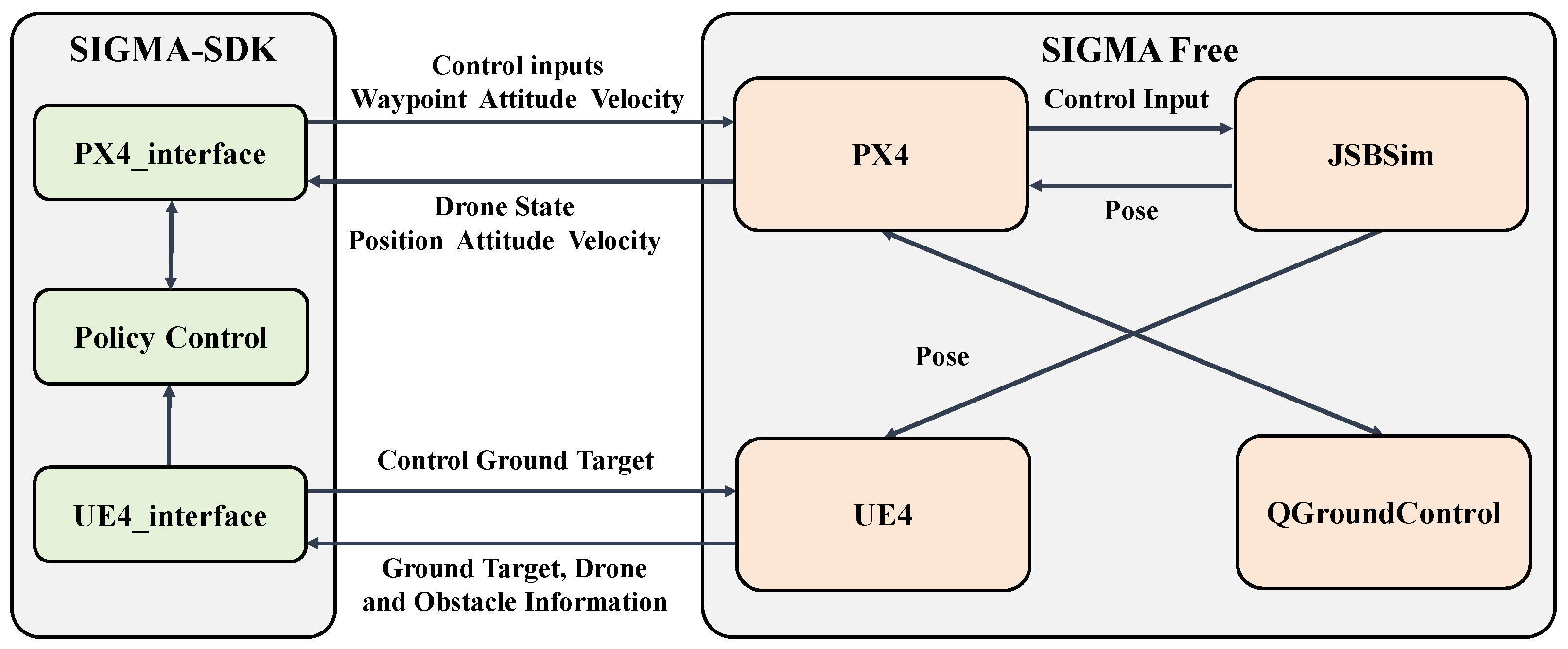
3.4.5. Simulation Environment

SIGMA (Swarm Intelligence General Machine Learning Environment for Unmanned Aerial Vehicles) [40] is an open-source and freely available simulation platform designed for low-altitude, slow-speed, and small rotorcrafts. The platform encompasses two fixed-wing aircraft and one quadrotor, with aerodynamic models refined through experimental data validation. The system integrates all algorithms within the flight controllers into the loop simulation, thereby ensuring that the relevant parameters and flight control mechanisms can be directly transferred to field testing scenarios.

Figure 6 shows the architecture of SIGMA Free. This system leverages UE4 as its rendering engine, providing detailed modeling and dynamic visualization of the aircraft’s physical and lighting characteristics, as well as the flight environment and target features. The software’s rendering video channel supports frame-by-frame image processing, thereby enabling the execution of more complex and intelligent tasks through deep learning techniques.

4. Experiments and Results

This chapter presents a detailed experimental validation and results analysis for our proposed VTD3. Firstly, the training process of the YOLOv8 model is outlined. Subsequently, the application of our VTD3 for the development of an advanced drone controller is demonstrated. Finally, through comparative experiments conducted in a simulated environment, the advantages of our proposed framework over traditional PD controllers in target tracking tasks are validated, with a particular emphasis on tracking accuracy and velocity smoothness.

4.1. YOLOv8 Model Training Process

4.1.1. Dataset

This study focuses on vehicle tracking in a simulated environment and constructs an extensive vehicle dataset specific to this simulation. To ensure data diversity and representativeness, we collect 400 images of vehicles under various lighting conditions, at various distances, at various altitudes, and in environmental contexts. Each image is standardized to a resolution of $1280\times 720$ pixels. The dataset comprises three typical scenarios: fully visible vehicles, partially occluded vehicles with the front half obstructed, and partially occluded vehicles with the rear half obstructed. Figure 7 presents representative examples of these three scenarios from our validation set. This design aims to comprehensively simulate a range of complex situations that may be encountered in practical applications, thereby enhancing the robustness of our tracking algorithm.

We use the Labelme tool (Labelme is an open-source Python package used for image annotation) for data annotation. For dataset partitioning, 40 images ($10\%$) are randomly chosen as the validation set, and the remaining 360 images ($90\%$) are used for training to ensure model generalization.

4.1.2. Model Configuration and Parameter Settings

We utilize the YOLOv8l model as our object detection method. The model is initialized with weights pre-trained on the COCO dataset to accelerate convergence speed. The training parameters are as follows: the total number of epochs is 300, with a batch size of 4 and an input image size of $640\times 640$. Stochastic Gradient Descent (SGD) is employed as the optimization algorithm, with a momentum of $0.937$ and a weight decay of $0.0005$. We use cosine annealing decay as our learning rate strategy, initiating at $0.01$ and progressively reducing to $0.0001$. Data augmentation techniques, such as random horizontal flips and scale transformations, are applied during the training process. Experiments are conducted on a machine equipped with an Intel i5-13400F CPU (Intel Corporation, Santa Clara, CA, USA) and an NVIDIA GeForce RTX 4070 Ti Super GPU (Nvidia, Santa Clara, CA, USA).

4.1.3. Evaluation Metrics

Precision and recall are essential metrics for the evaluation of object detection models. Precision measures the accuracy of the model’s predictions, whereas recall evaluates the model’s capability to identify all pertinent instances. These metrics are computed as follows:

$$\mathrm{Precision}={\displaystyle \frac{\mathrm{TP}}{\mathrm{TP}+\mathrm{FP}}}$$

(13)

$$\mathrm{Recall}={\displaystyle \frac{\mathrm{TP}}{\mathrm{TP}+\mathrm{FN}}}$$

(14)

where TP, FP, and FN represent true positives, false positives, and false negatives, respectively.

The metrics ${\mathrm{mAP}}_{50}$ and ${\mathrm{mAP}}_{50-95}$ provide a more comprehensive evaluation by considering the performance across the entire precision–recall curve. Specifically, ${\mathrm{mAP}}_{50}$ refers to the mean Average Precision at an IoU threshold of $50\%$, whereas ${\mathrm{mAP}}_{50-95}$ represents the average of mAP values computed over the IoU range from $50\%$ to $95\%$ with increments of $5\%$. N is the number of classes; $p_{i,50}\left(r\right)$ is the precision for the i-th class at a recall r with an IoU threshold of $50\%$; and $p_{i,j}\left(r\right)$ is the precision function for the i-th class at a recall r with an IoU threshold of $(45+5j)\%$. The calculation of these metrics can be expressed in integral form as follows:

$${\mathrm{mAP}}_{50}={\displaystyle \frac{1}{N}}\sum _{i=1}^N{\int }_0^1{p}_{i,50}\left(r\right)dr$$

(15)

$${\mathrm{mAP}}_{50-95}={\displaystyle \frac{1}{10}}\sum _{j=5}^{10}\left[{\displaystyle \frac{1}{N}}\sum _{i=1}^N{\int }_0^1{p}_{i,j}\left(r\right)dr\right]$$

(16)

These metrics provide a comprehensive evaluation of the model’s performance across varying detection accuracy requirements by calculating the area under the precision–recall curve at various IoU thresholds.

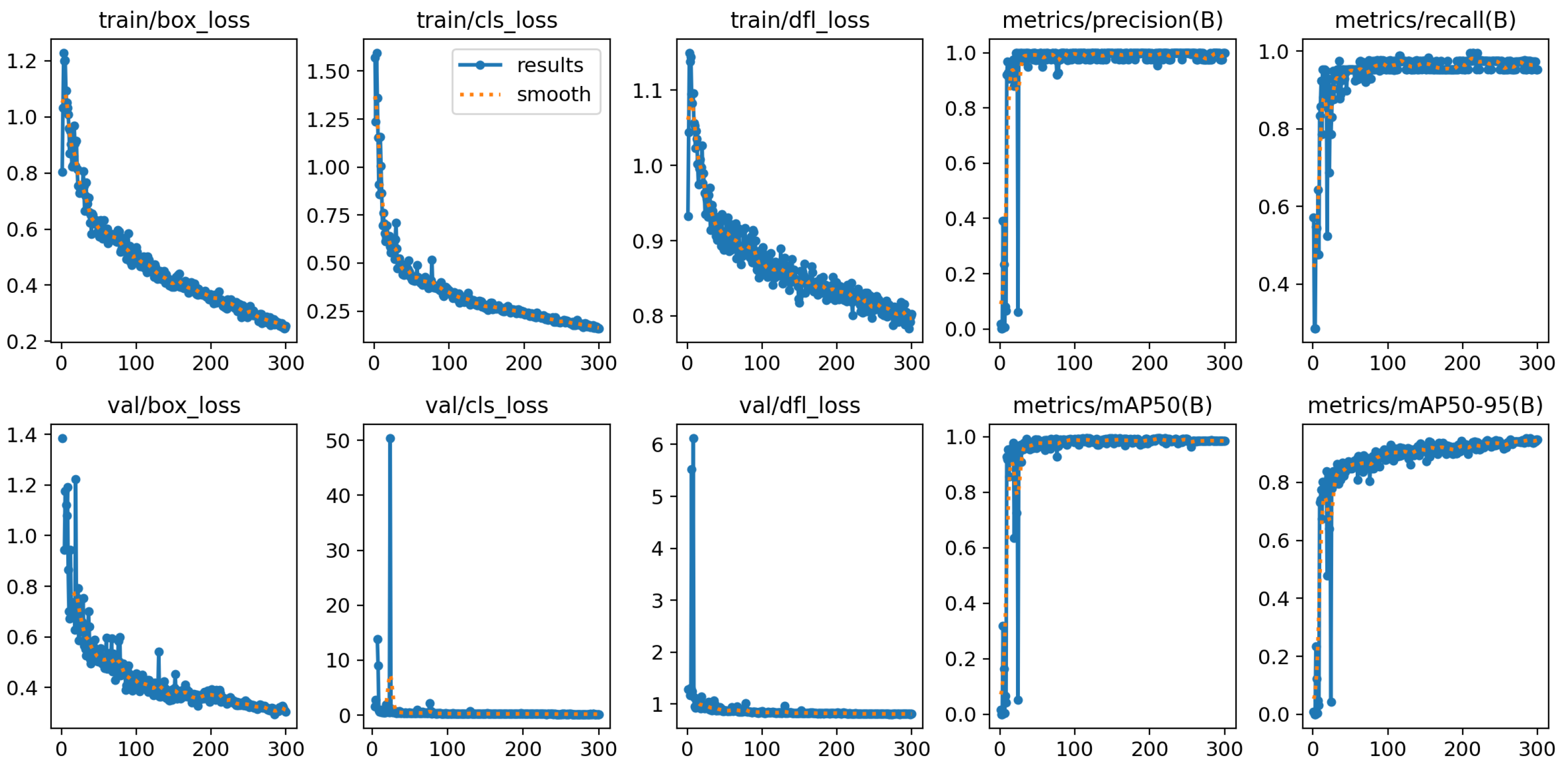
4.1.4. YOLOv8 Model Training Results

Figure 8 depicts the training results of YOLOv8. It is evident that an increase in the number of training epochs correlates with a marked enhancement in the model’s performance on both the training and validation datasets. Notably, the three primary loss functions demonstrate a consistent decline, while evaluation metrics (precision, recall, ${\mathrm{mAP}}_{50}$, and ${\mathrm{mAP}}_{50-95}$) exhibit progressive improvement throughout the training process.

Figure 9 shows the detection results of representative samples from three typical scenarios in the validation set. The model accurately detects vehicles across all scenarios, exhibiting high confidence scores (Unoccluded: $0.94$, Rear Occluded: $0.93$, Front Occluded: $0.89$). These results suggest that YOLOv8 effectively learns the salient visual features of vehicles during the training phase, demonstrating robust performance even under challenging conditions such as partial occlusion. The model’s robustness across various scenarios provides a reliable foundation for subsequent drone-based vehicle tracking applications.

The observed consistent trend of performance enhancement robustly signifies the efficacy of the model’s learning process. In particular, the network progressively acquires the critical appearance features of vehicles, enabling it to execute accurate detection and classification across diverse and complex scenarios. Importantly, the sustained improvement in performance on the validation set indicates that the model possesses strong generalization capabilities.

It is important to note that these results are based on training and validation using virtual images collected from a simulated environment. Our proposed VTD3 demonstrates high accuracy in this simulated setting. Some studies have shown that virtual datasets can effectively assist in solving many practical problems and improve their performance [41,42]. Indeed, performance may differ in real-world situations due to additional complexities and variations not present in the simulation. Factors such as lighting conditions, weather effects, and the diversity of real-world vehicle appearances could potentially impact the detection accuracy. Future work may involve testing and fine-tuning the model on real-world data to improve its performance in practical applications.

4.2. TD3 Network Training Process

4.2.1. TD3 Network Training Framework and Strategy

This research devises a vision-based end-to-end reinforcement learning framework VTD3 for drone target tracking control. The framework integrates computer vision methodologies with deep reinforcement learning algorithms to achieve efficient autonomous drone control. The core framework pipeline is as follows:

• Visual Perception: The drone captures real-time video streams via its onboard camera and processes the current frame using a YOLOv8 object detection algorithm.
• Target Tracking: The detection results are fed into a BoT-SORT tracker, enabling continuous target identification and verification.
• State Representation: Based on the detected target information (the bbox coordinates), the system computes and generates a state vector.
• Action Generation: The state vector is input into the TD3 network, which outputs control actions for the drone, including forward/backward and left/right control magnitudes.
• Reward Calculation and Learning: The system computes reward values based on the current state and executed actions. Information pertaining to state, action, and reward is archived in an experience replay buffer for network training and policy optimization.
• Action Execution: Control commands, generated by the TD3 network, are transmitted to the drone’s PX4 flight control system, which subsequently modulates the rotational speed of the four rotors to implement the specified actions.
• Environmental Interaction: The drone performs actions within the simulation environment and acquires new image data via its onboard camera, thereby initiating the subsequent processing cycle.
• Iterative Optimization: The system perpetually executes the aforementioned pipeline, progressively improving the target tracking performance of the TD3 controller through iterative interactions and learning.

To enhance learning efficiency and policy robustness, we employ a three-stage training strategy:

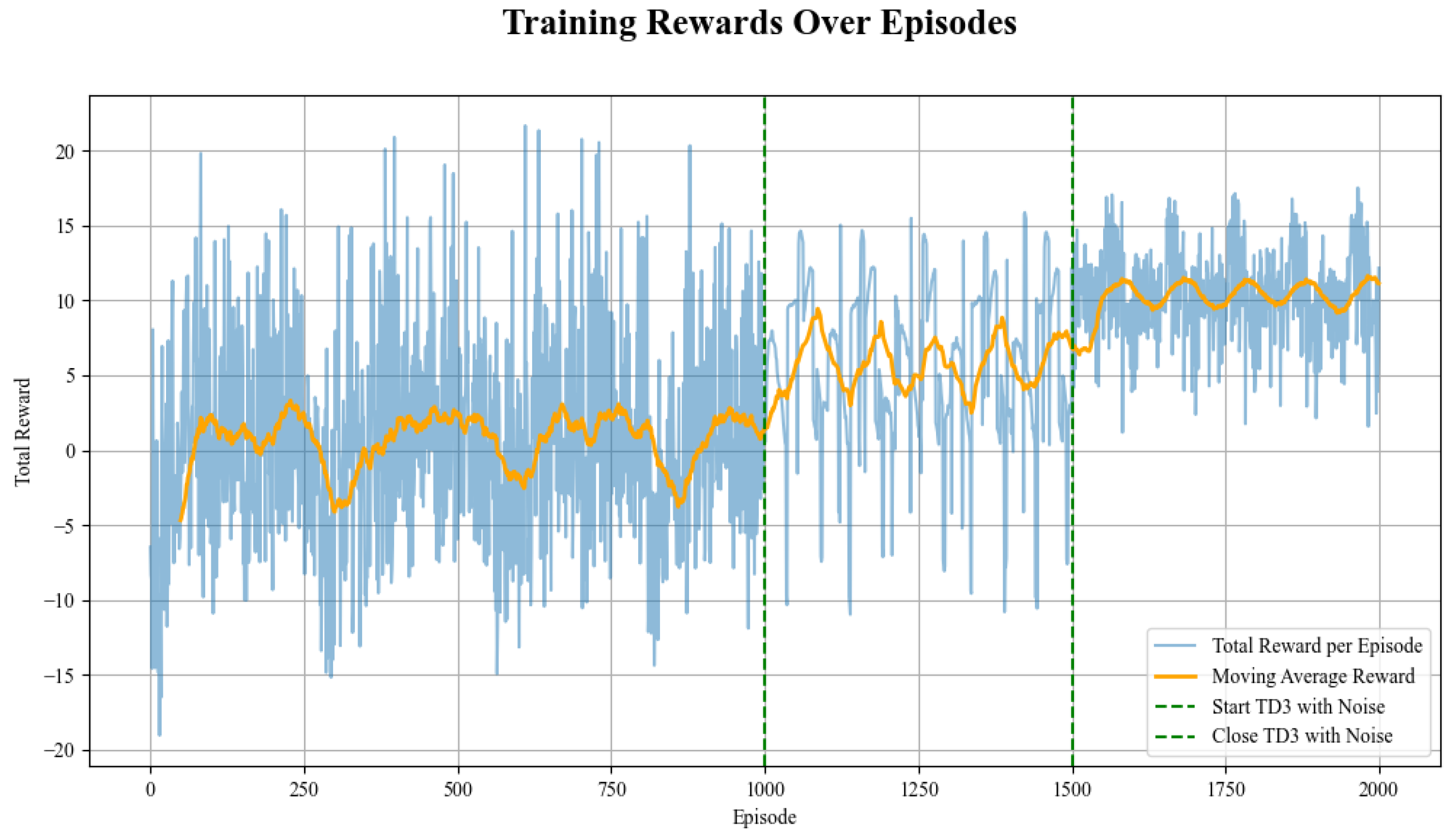
• Random Exploration Stage: This stage involves the TD3 network generating random control actions. This phase is designed to comprehensively explore the state space, thereby gathering a diverse set of experiential data that serves as a foundational basis for subsequent learning stages.
• Noisy Exploration Stage: As training advances, the TD3 network starts to produce intentional control actions. To enhance the learning process, Gaussian noise is introduced to the network’s output actions. This strategy effectively balances exploration and exploitation, thereby augmenting the diversity of data in the experience replay buffer and enabling the network to learn more robust control policies.
• Pure Policy Stage: During the final training stage, the TD3 network autonomously generates control actions without additional noise. This phase is dedicated to policy optimization, enabling the network to leverage the experiential knowledge acquired in the preceding stages to fine-tune the optimal control strategy.

To further enhance the model’s generalization capability, we periodically alter the target vehicle’s position within the drone’s field of view every 100 time steps. This dynamic environment setup ensures a diverse set of training data, thereby enhancing the network’s ability to learn more generalized and robust tracking strategies. To provide a comprehensive understanding of our framework and to elucidate the precise implementation of the TD3 algorithm within our multi-stage training strategy, we present the following pseudocode of the core algorithm in Algorithm 1:

Algorithm 1 TD3: Vision-Based End-to-End TD3 Reinforcement Learning Method

1: procedure Initialize   2:     MAX_STEPS ← Set maximum number of steps   3:     RANDOM_STEPS ← Set steps for random exploration   4:     TD3_NOISE_STEPS ← Set steps for TD3 with noise   5:     TD3_STEPS ← Set steps for pure TD3   6:     UPDATE_INTERVAL ← Set update interval   7:     agent ← Initialize TD3 agent   8:     buffer ← Initialize experience replay buffer   9: end procedure 10:    11: procedure TrainAgent 12:     frameSteps ← 0 13:     while frameSteps < MAX_STEPS do 14:       state ← GetStateFromYOLOv8() 15:       if frameSteps < RANDOM_STEPS then 16:           action ← RandomAction() 17:       else if frameSteps < TD3_NOISE_STEPS then 18:           action ← TD3ActionWithNoise(state) 19:       else if frameSteps < TD3_STEPS then 20:           action ← TD3Action(state) 21:       end if 22:       ExecuteAction(action) // Send Mavlink message 23:       new_state ← ObserveNewState() 24:       reward ← CalculateReward() 25:       buffer.Add(state, action, reward, new_state) 26:       if frameSteps % UPDATE_INTERVAL $==0$ and frameSteps $\ge 2\ast$ UPDATE_INTERVAL then 27:           agent.Update(buffer) 28:       end if 29:       frameSteps ← frameSteps + 1 30:     end while 31: end procedure 32:    33: procedure Main 34:     Initialize() 35:     TrainAgent() 36: end procedure

4.2.2. Simulation Platform and Parameter Settings

In the simulation environment of this study, we employ the F450 quadrotor drone as the experimental platform. The F450 is a widely used classic quadrotor design, distinguished by its “X”-shaped frame and a 450 mm wheelbase, which offers superior stability and reliability. Within our simulation model, the F450 is equipped with the PX4 flight control system serving as the low-level controller. This configuration leverages the PX4’s fundamental flight stabilization capabilities, thereby establishing a dependable foundation for our investigation into advanced control algorithms.

Table 2. Parameters of the TD3 algorithm.

Parameter Name	Value
Hidden layer number	2
Hidden layer width	64
Dimension of states	2
Dimension of actions	2
Max_action	6 m/s
Control period	0.3 s
Buffer size	${10}^6$
Batch size	64
MAX_STEPS	2000
RANDOM_STEPS	1000
TD3_NOISE_STEPS	500
TD3_STEPS	500
UPDATE_INTERVAL	50
Optimizer	Adam
Learning rate for actor networks	0.001
Learning rate for Q networks	0.001
Discount factor	0.99
Explore_noise	0.15
Explore_noise_decay	0.998

provides the hyperparameter values employed during the training phase of the TD3 algorithm. Each time step is set to $0.3$ s, which includes the duration required for target detection. Empirical observations indicate that the interval from target detection in the video stream to action generation is approximately $0.05$ s, whereas the execution time for the drone’s actions is about $0.25$ s. This temporal distribution ensures that the low-level controller is allotted adequate time to execute actions effectively, thereby minimizing tracking delays.

In terms of network architecture, we employ two hidden layers, each consisting of 64 hidden units. For both the actor network and the Q network, the learning rate is set to $0.001$. Given that both the state space and action space are two dimensional, this network configuration enables rapid convergence to the optimal policy while mitigating the risks associated with prolonged training times and overfitting, which may result from an excessive number of layers or hidden units. This balanced parameter selection enhances the network’s learning efficiency and generalization capability.

4.2.3. TD3 Network Training Results

Figure 10 illustrates the evolution of the total rewards throughout the training process of the TD3 network. The x-axis represents the number of training episodes, while the y-axis indicates the total reward per episode. The blue curve represents the total reward for each individual episode, and the yellow curve signifies the moving average of total rewards, which serves to smooth short-term fluctuations and emphasize long-term trends.

During the initial phase of random exploration, encompassing the first 1000 episodes, the total reward demonstrates considerable variability, accompanied by a relatively low moving average. This phenomenon can be attributed to the network’s emphasis on random exploration. The aim is to thoroughly comprehend the state–action space pertinent to the target tracking task. As training progresses, the TD3 algorithm introduces noise for exploration between episodes 1000 and 1500. During this interval, there is a noticeable increase in the moving average reward, suggesting that the introduction of noise aids the network in obtaining higher rewards during the exploration process.

After 1500 episodes, the network primarily operates based on the learned policy. The volatility in total rewards decreases, and the moving average reward improves and stabilizes, further indicating that the network has identified an optimal control strategy for the target tracking task. These findings corroborate the efficacy of the TD3 for this task. They illustrate how the algorithm incrementally enhances the drone’s control performance in target tracking. This improvement occurs through three phases: an initial phase of random exploration, followed by noise-assisted exploration in the intermediate phase, and culminating in pure policy operation. Ultimately, this process achieves high and stable rewards.

4.3. Comparative Experiments

4.3.1. Experimental Setup

We perform a comparative evaluation of TD3 and PD controllers for drone-based visual target tracking tasks in a simulated environment. To rigorously validate the efficacy of the TD3 controller in tracking nonlinear motions, as illustrated in Figure 11, we design four distinct vehicle motion trajectories: triangular, square, sawtooth, and square wave. Notably, the square wave trajectory includes three instances of target occlusion, thereby simulating the complex visual disturbances commonly encountered in real-world scenarios. The experimental setup is as follows:

• Initial Conditions:
  • Vehicle starting position: (30 m, 100 m, 0 m);
  • Drone initial position: (30 m, 60 m, 4 m);
  • To simulate real-world hovering instabilities, the drone’s actual initial position in the simulation is subjected to a maximum random deviation of $1\%$ from the ideal position.
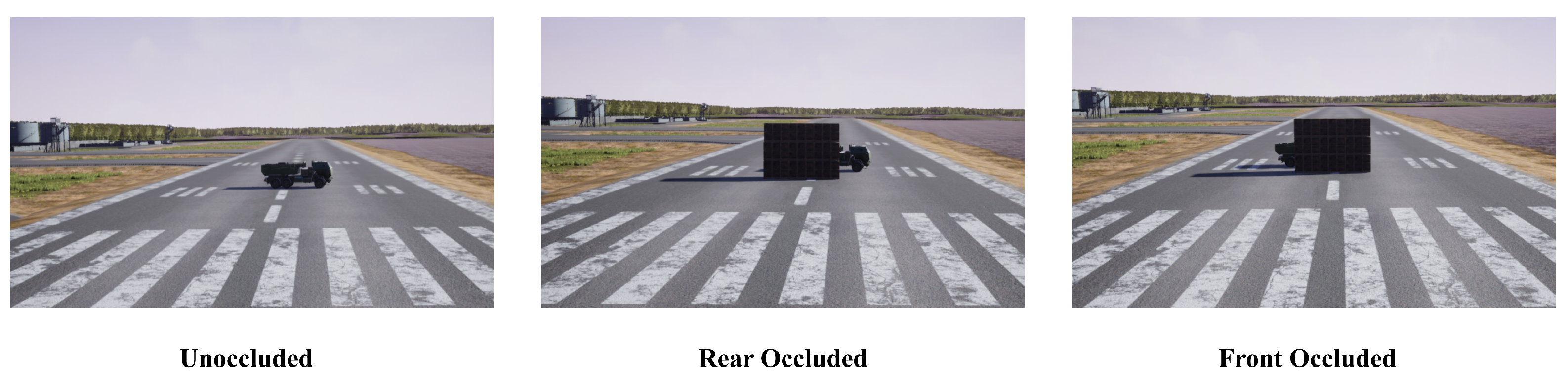
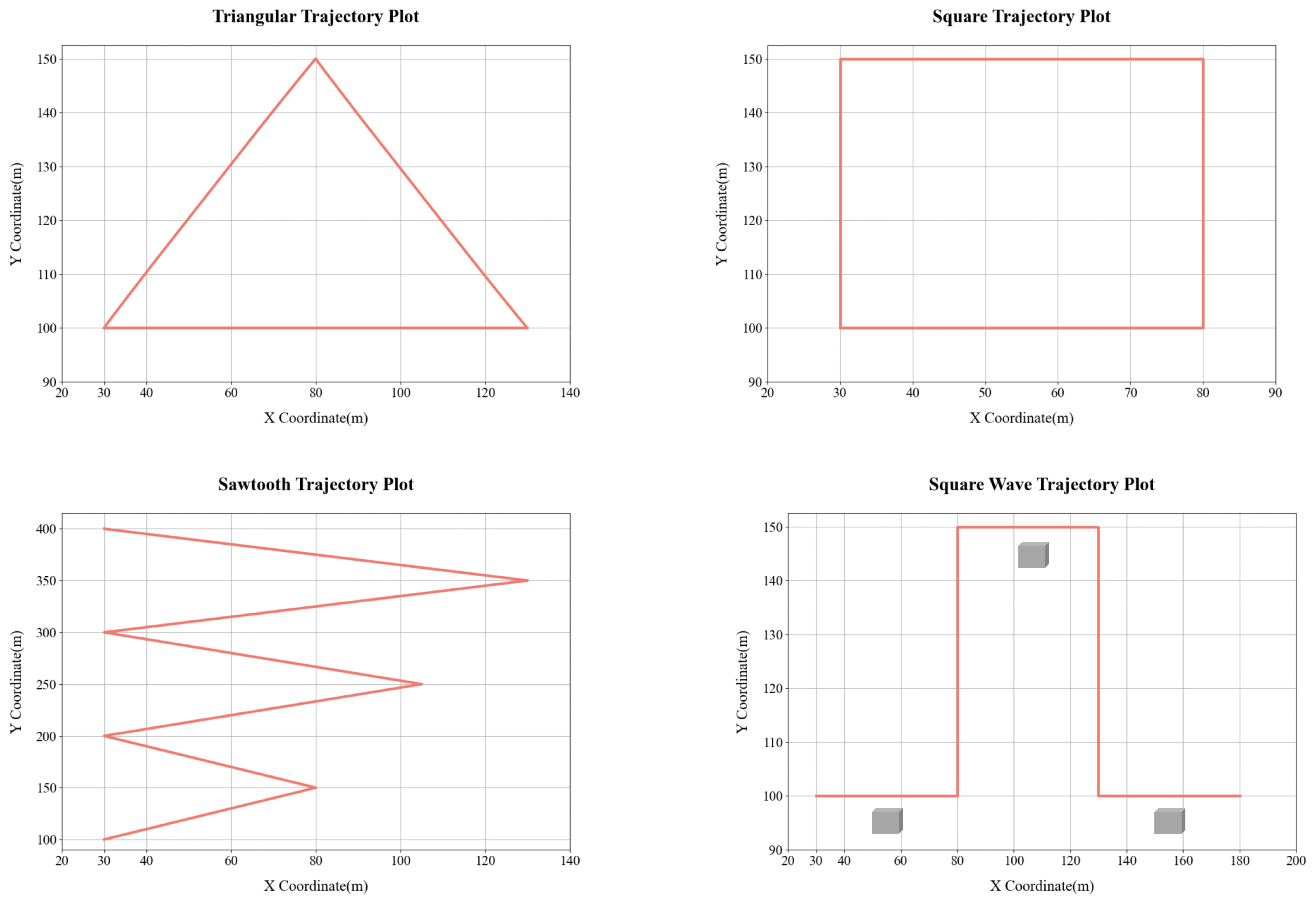
• Occlusion Setup:

   

  For the square wave trajectory, three occlusion walls are strategically positioned:

  •

  Position 1: (55 m, 95 m, 0 m);

  •

  Position 2: (105 m, 145 m, 0 m);

  •

  Position 3: (155 m, 105 m, 0 m).

   

  Each occlusion wall measures 8 m in width and 5 m in height, designed to create

   

  realistic visual obstruction scenarios.
• Vehicle Trajectory Design:
  • The simulated vehicle’s trajectory consists of multiple consecutive start–end segments, each completed in a fixed duration of $16.5$ s. Each segment adheres to a standard three-phase motion pattern: uniform acceleration, constant velocity, and uniform deceleration, mimicking typical vehicular movement characteristics. After completing each motion segment, the vehicle undergoes a 2 s pause to alter its direction. This segmented design enables the construction of complex overall trajectories (such as triangular, square, sawtooth, and square wave patterns) while ensuring uniformity within each motion segment. Consequently, it offers a dependable benchmark for assessing the performance of drone tracking controllers across a variety of motion scenarios.

This experimental design seeks to rigorously evaluate the visual tracking accuracy, system stability, and environmental adaptability of both controllers across trajectories of varying complexity. Additionally, by introducing visual disturbances such as target occlusion, we further investigate the robustness of the controllers under conditions of uncertainty and intermittent image data.

4.3.2. Evaluation Metrics

To comprehensively evaluate the performance of the TD3 and PD controllers in drone visual target tracking tasks, this study employs five key indicators:

• X-Axis Average Tracking Error ($X_{dif}$)
  • This metric reflects the tracking precision of the drone in the lateral direction. We record the positions of both the vehicle and the drone at 0.1 s intervals. We then compute the mean absolute difference in their X-axis positions across the entire trajectory. N denotes the total number of samples, and x_drone,i and x_target,i represent the X-coordinates of the drone and target vehicle at the i-th sample, respectively. A lower X_dif value signifies higher precision in lateral tracking. The formula is defined as follows:

    $$X_{dif}={\displaystyle \frac{1}{N}}\sum _{i=1}^N|x_{drone,i}-x_{vehicle,i}|\left(m\right)$$

    (17)
• Y-Axis Average Tracking Error ($Y_{dif}$)
  • This metric evaluates the drone’s ability to sustain a specified tracking distance along the longitudinal axis. The computational approach parallels that of X_dif but with a target value set at 40 m. The proximity of Y_dif to 40mserves as an indicator of the controller’s precision in maintaining the designated tracking distance, thereby reflecting enhanced control performance. The formula is as follows:

    $$Y_{dif}={\displaystyle \frac{1}{N}}\sum _{i=1}^N|y_{drone,i}-y_{vehicle,i}-40|\left(m\right)$$

    (18)
• Z-Axis Average Altitude Error ($Z_{dif}$)
  • This metric quantifies the mean absolute deviation of the drone’s actual flight altitude from the initial set altitude of 4 m. Despite the lack of direct altitude control in the experiment, variations in altitude still arise due to the inherent dynamics of the quadrotor drone during planar motion execution. A smaller Z_dif value indicates higher precision and the superior dynamic compensation capability of the controller during complex planar maneuvers. The formula is as follows:

    $$Z_{dif}={\displaystyle \frac{1}{N}}\sum _{i=1}^N|z_{drone,i}-4|\left(m\right)$$

    (19)
• Velocity Jitter Metric ($J_v$)
  • The velocity jitter metric quantifies the extent of rapid velocity fluctuations over brief temporal intervals. In this study, utilizing velocity data sampled at 0.1 s intervals, it is determined by calculating the standard deviation of the first-order difference in velocity across the entire duration of observation. Let v_i be the velocity at the i-th sample. A lower mean value of the velocity jitter indicates smoother overall motion, reflecting the controller’s ability to maintain stable velocity changes. The formula is as follows:

    $$J_v=\sqrt{{\displaystyle \frac{1}{N-1}}\sum _{i=1}^{N-1}{(v_{i+1}-v_i)}^2}(m/s)$$

    (20)
• Jerk Root Mean Square Metric ($J_{RMS}$)
  • The Jerk Root Mean Square (Jerk RMS) indicator is the root mean square value of the time derivative of acceleration, thereby reflecting the intensity of the variations in acceleration. This metric is derived by computing the root mean square of the second-order differences in velocity data, utilizing a sampling interval of 0.1 s. Let Δt be the time interval between samples (0.1 s in this study). A lower average Jerk RMS value indicates the controller’s capability to produce smoother acceleration changes, thus enhancing the fluidity and efficiency of motion control. The formula for Jerk RMS is as follows:

    $$J_{RMS}=\sqrt{{\displaystyle \frac{1}{N-2}}\sum _{i=1}^{N-2}{\left({\displaystyle \frac{v_{i+2}-2v_{i+1}+v_i}{{(\Delta t)}^2}}\right)}^2}(m/s^3)$$

    (21)

These five indicators form a comprehensive evaluation system encompassing spatial position accuracy, motion smoothness, and control stability. By comparing the performance of various controllers across these metrics, we can rigorously assess their efficacy in complex visual target tracking tasks. Lower error values and motion indicators generally suggest that a controller exhibits higher precision, better stability, and smoother motion characteristics, which are crucial for practical target tracking applications.

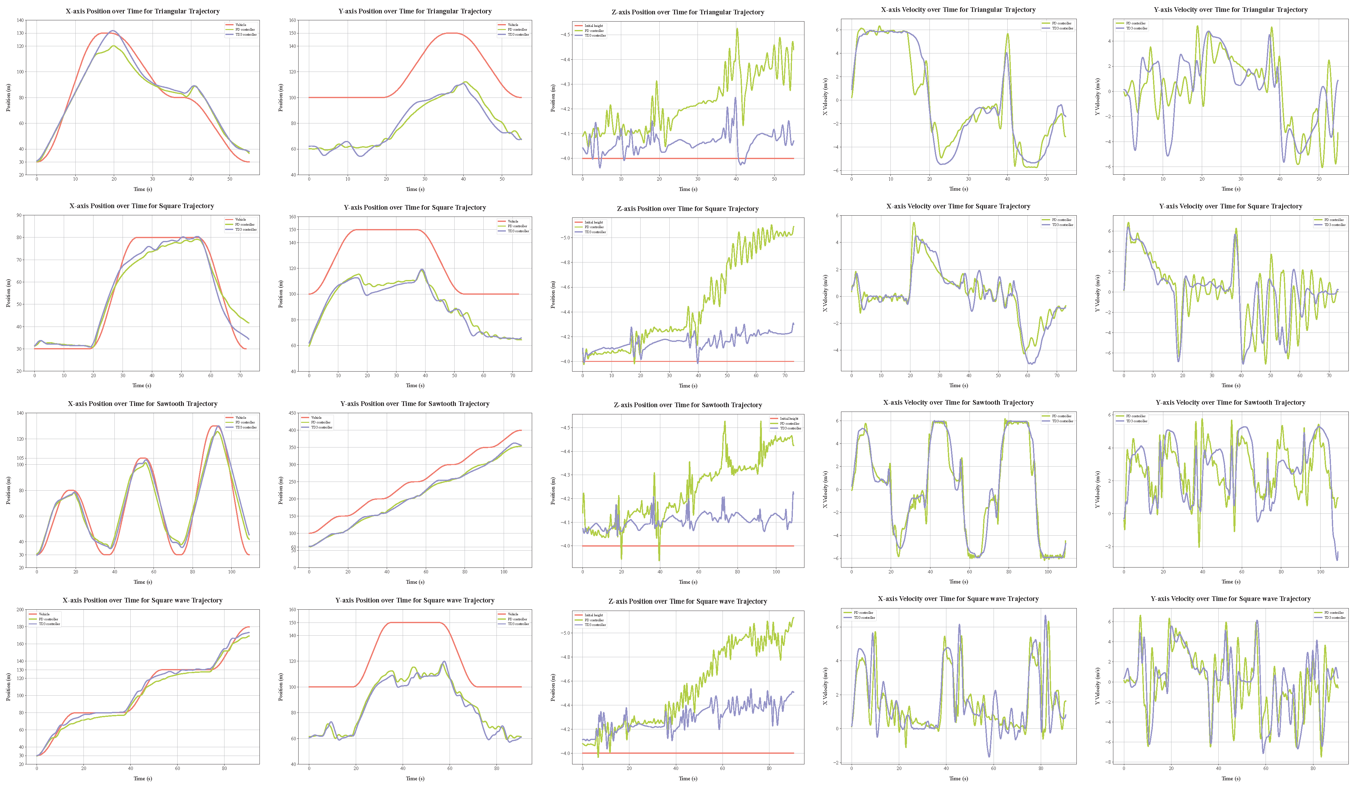
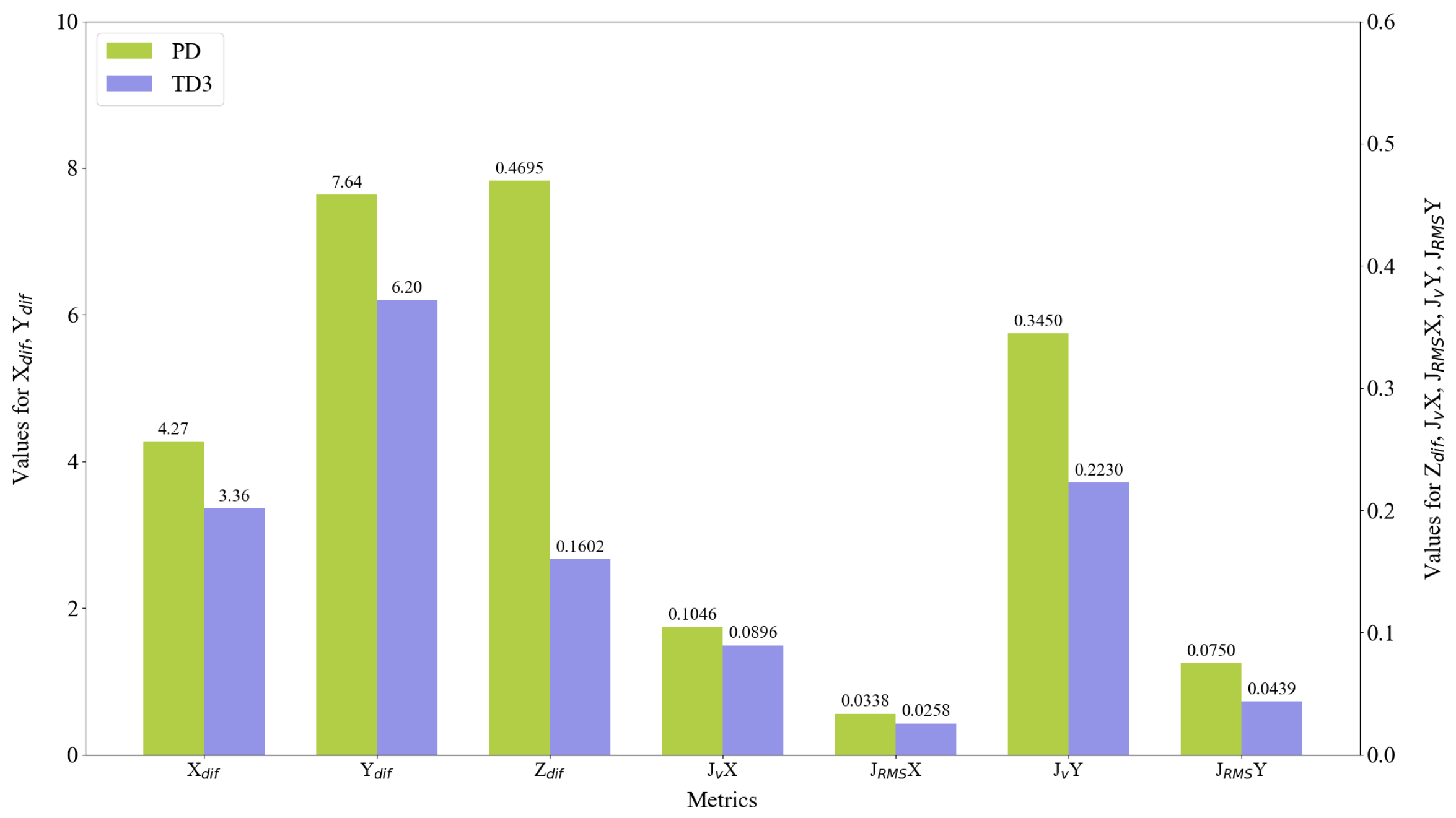
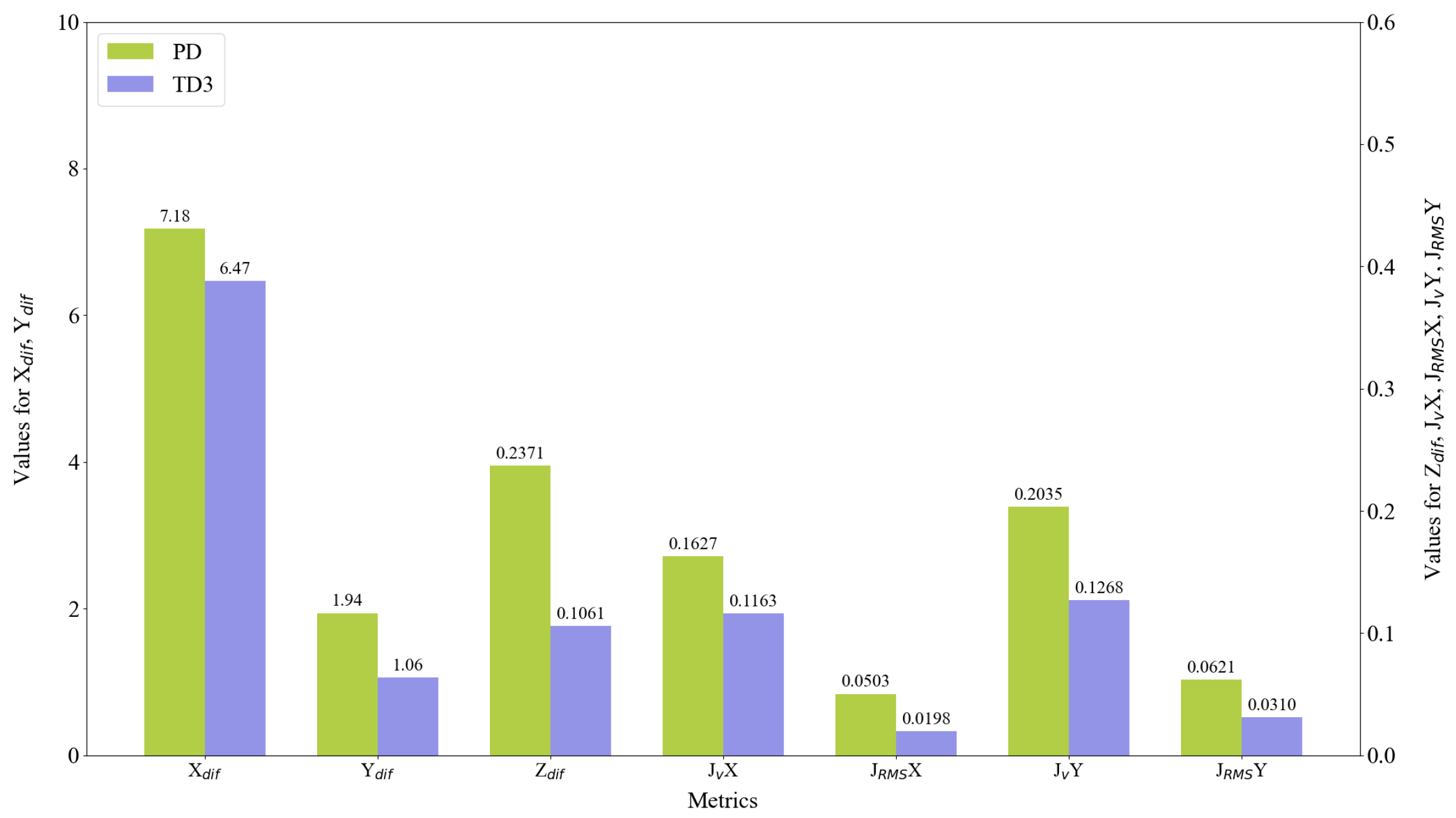
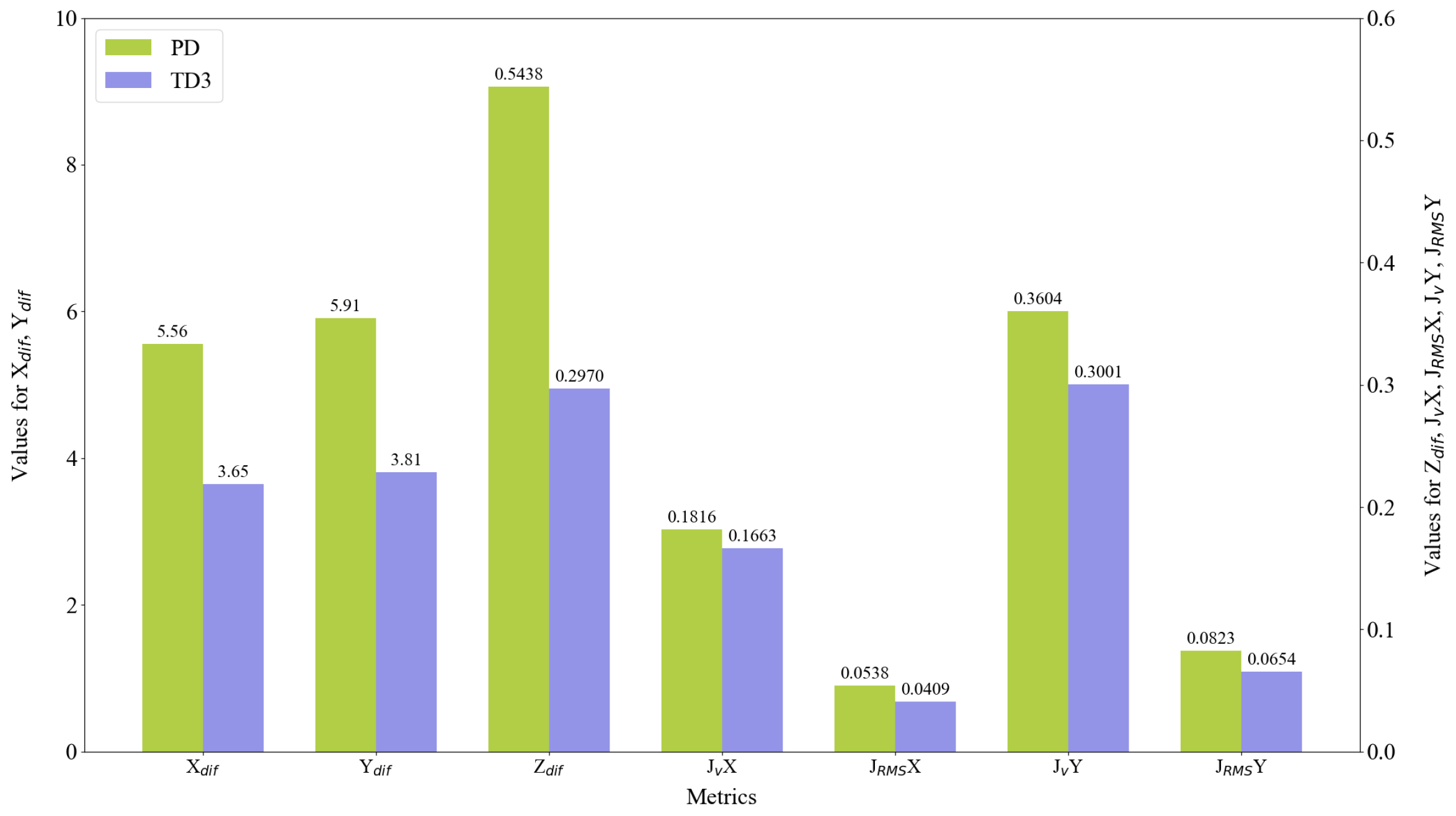
4.3.3. Comparative Experiments Results

Figure 12 presents the results of position–time relationships for the X- and Y-axis across the four trajectories. It indicates that the TD3 controller exhibits superior tracking accuracy relative to the PD controller. The temporal variations in altitude along the Z-axis underscore a notable enhancement in altitude stability when utilizing the TD3 controller. This improvement can be ascribed to the TD3 algorithm’s adaptability and its ability to optimize complex nonlinear systems.

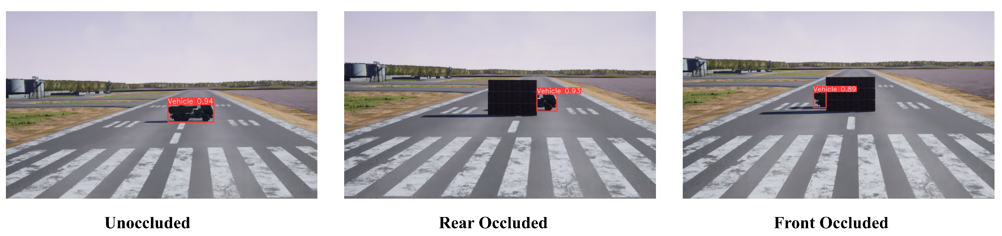
Qualitative Analysis

Regarding velocity control, the TD3 controller exhibits a more assertive approach while maintaining smoother velocity curves, indicating more stable drone control. This attribute can be attributed to the design of the reward function employed during the TD3 training process. The reward function not only incentivizes a rapid approach to the target but also promotes stability upon nearing the target, thereby achieving an optimal balance between speed and stability.

It is important to note that, during the vehicle turning phases, the drone’s motion trajectory exhibits a certain degree of deviation. This primarily arises from the pure vision-based method employed in this study, which estimates the vehicle’s distance along the Y-axis by analyzing the area of the target detection box. When the vehicle turns, the area of the detection box inevitably changes, resulting in errors in distance estimation and subsequently impacting the drone’s tracking accuracy. This phenomenon highlights the limitations of vision-based distance estimation in dynamic scenarios.

Quantitative Analysis of Four Trajectory Types

The experimental results for the different scenarios are presented in Figure 13, Figure 14, Figure 15 and Figure 16. In these figures, the blue curves represent the TD3 controller, and the green curves represent the PD controller. The left Y-axis corresponds to $X_{dif}$ and $Y_{dif}$, while the right Y-axis corresponds to $Z_{dif}$, $J_v$, and $J_{RMS}$. The units for $X_{dif}$, $Y_{dif}$, and $Z_{dif}$ are meters (m), $J_v$ is in meters per second (m/s), and $J_{RMS}$ is in meters per second cubed (m/s³).

(1)

Tracking Accuracy and Trajectory Characteristics Analysis

• X-axis direction: The TD3 controller outperforms the PD controller in all trajectories. The improvement ranges from a minimum of 9.89% (Figure 15) for the sawtooth trajectory to a maximum of 34.35% (Figure 16) for the square wave trajectory, with an average improvement of 20.20%.
• Y-axis direction: The TD3 similarly demonstrates advantages. The improvement ranges from 18.85% (Figure 14) for the square trajectory to 45.36% (Figure 15) for the sawtooth trajectory, with an average improvement of 32.08%.
• Z-axis direction (altitude control): The TD3 shows the most significant improvement. The minimum improvement is 45.38% (Figure 16) for the square wave trajectory, while the maximum is 70.38% (Figure 13) for the triangular trajectory, with an average improvement of 59.22%.

(2)

Motion Smoothness Analysis

• X-axis velocity jitter ($J_{v}X$): The TD3 reduces velocity jitter in all trajectories. The minimum improvement is 8.42% (Figure 16) for the square wave trajectory, while the maximum is 36.01% (Figure 13) for the triangular trajectory, with an average improvement of 21.82%.
• X-axis jerk ($J_{RMS}X$): The TD3 also improves jerk. The minimum improvement is 23.67% (Figure 14) for the square trajectory, while the maximum is 60.64% (Figure 15) for the sawtooth trajectory, with an average improvement of 38.82%.
• Y-axis velocity jitter ($J_{v}Y$): The TD3 similarly reduces velocity jitter in the Y-axis direction. The minimum improvement is 16.73% (Figure 16) for the square wave trajectory, while the maximum is 37.70% (Figure 15) for the sawtooth trajectory, with an average improvement of 27.90%.
• Y-axis jerk ($J_{RMS}Y$): The TD3 also shows improvement in reducing Y-axis jerk. The minimum improvement is 20.53% (Figure 16) for the square wave trajectory, while the maximum is 50.08% (Figure 15) for the sawtooth trajectory, with an average improvement of 36.26%.

(3)

Comprehensive Analysis

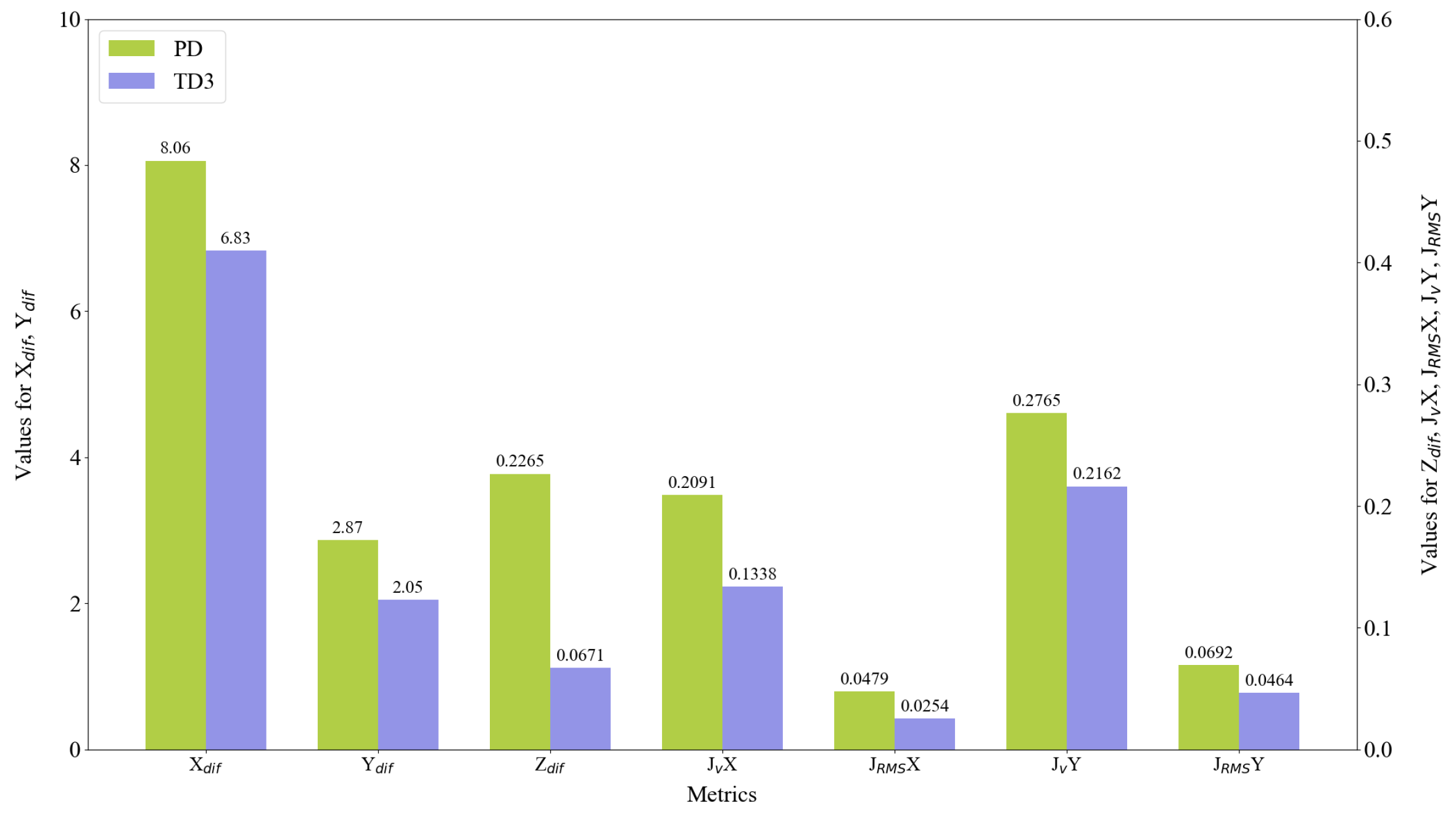
• The TD3 controller outperforms the PD controller in all evaluation metrics, demonstrating significant advantages in complex trajectory tracking tasks.
• Altitude control (Z-axis) shows the most substantial improvement, with an average of 59.22%, which is crucial for maintaining a stable tracking perspective.
• The reduction in velocity jitter is also notable, especially in the Y-axis direction, with an average improvement of 27.90%, contributing to enhanced flight stability and energy efficiency.
• In the square wave trajectory, which includes target occlusion scenarios, the TD3 maintains significant performance advantages, particularly in XY-plane tracking accuracy (a 34.35% and 35.52% improvement, respectively), demonstrating strong robustness and adaptability.
• In the sawtooth trajectory, the TD3 performs best in Y-axis tracking accuracy and X-axis velocity jerk reduction, with improvements of 45.36% and 60.64%, respectively, indicating its superior handling of frequent direction changes.
• For the square trajectory, the TD3 shows the greatest improvement in Z-axis control (66.10%), suggesting its particular effectiveness in scenarios requiring stable altitude maintenance.

5. Conclusions and Discussion

Based on the TD3 algorithm, this paper proposes a vision-based end-to-end reinforcement learning framework, VTD3, for drone target tracking tasks. When evaluated across four complex trajectories—triangular, square, sawtooth, and square wave with occlusions—the TD3 controller significantly outperforms the traditional PD controller. Experimental results indicate that the TD3 algorithm reduces average tracking errors by up to 34.35% and 45.36% on the X- and Y-axis, respectively, while achieving a remarkable 70.38% improvement in altitude control precision.

Regarding motion smoothness, the TD3 algorithm exhibits substantial advancements, achieving improvements of up to 37.70% in jitter metrics and 60.64% in Jerk RMS indicators. These enhancements not only significantly improve tracking accuracy but also markedly enhance motion smoothness, which is critical for advancing drone performance in purely vision-based tracking tasks. Specifically, in managing complex trajectories and occlusion scenarios, the TD3 controller’s demonstrated adaptability and robustness make it a compelling choice for vision-based tracking applications.

The TD3 controller demonstrates a substantial enhancement in altitude control, with an average improvement of $59.22\%$. This advancement not only enhances tracking performance but also holds potential benefits for other applications that depend on stable flight platforms, including aerial photography and precision mapping. In terms of motion smoothness, the TD3 controller significantly mitigates velocity jitter and jerk, resulting in smoother motion characteristics. This improvement in tracking efficiency may also confer additional advantages, such as reduced energy consumption and extended flight duration.

Nonetheless, the study also identifies limitations inherent to purely vision-based methods in dynamic environments, particularly noting trajectory deviations during vehicle turning phases. This finding underscores the persistent challenges in the field of visual navigation. Future research directions may encompass the exploration of multi-sensor fusion technologies to improve distance estimation accuracy and the investigation of efficient implementations of complex reinforcement learning algorithms on physical hardware. These advancements are poised to significantly enhance the capabilities of autonomous drone systems operating in complex environments, concurrently offering novel insights into the mitigation of computational complexity and resource constraints in practical applications.

Future research in this domain will focus on two main directions. Firstly, we aim to explore more precise depth estimation techniques using RGB images, moving beyond the current use of the YOLOv8 detection box area as a proxy for target distance. The goal is to achieve accurate distance estimation without significantly increasing computational load, potentially through advanced computer vision algorithms or lightweight depth estimation networks.

Secondly, bridging the gap between simulation and real-world environments is crucial. This involves fine-tuning the YOLOv8 model on real-world data and enhancing the TD3 algorithm’s control capabilities in diverse visual environments, accounting for varying lighting, weather, and dynamic obstacles. These efforts aim to ensure system robustness in practical applications.

References

- Aliloo, J.; Abbasi, E.; Karamidehkordi, E.; Parmehr, E.G.; Canavari, M. Dos and Don’ts of using drone technology in the crop fields. Technol. Soc. 2024, 76, 102456. [Google Scholar] [CrossRef]
- Liu, H.; Tsang, Y.; Lee, C. A cyber-physical social system for autonomous drone trajectory planning in last-mile superchilling delivery. Transp. Res. Part C Emerg. Technol. 2024, 158, 104448. [Google Scholar] [CrossRef]
- Khosravi, M.; Arora, R.; Enayati, S.; Pishro-Nik, H. A search and detection autonomous drone system: From design to implementation. IEEE Trans. Autom. Sci. Eng. 2024, 1–17. [Google Scholar] [CrossRef]
- Aboelezz, A.; Wetz, D.; Lehr, J.; Roghanchi, P.; Hassanalian, M. Intrinsically Safe Drone Propulsion System for Underground Coal Mining Applications: Computational and Experimental Studies. Drones 2023, 7, 44. [Google Scholar] [CrossRef]
- Sheng, H.; Chen, G.; Xu, Q.; Li, X.; Men, J.; Zhou, L.; Zhao, J. An advanced gas leakage traceability & dispersion prediction methodology using unmanned aerial vehicle. J. Loss Prev. Process. Ind. 2024, 88, 105276. [Google Scholar]
- Ardiny, H.; Beigzadeh, A.; Mahani, H. Applications of unmanned aerial vehicles in radiological monitoring: A review. Nucl. Eng. Des. 2024, 422, 113110. [Google Scholar] [CrossRef]
- Do, T.T.; Ahn, H. Visual-GPS combined ‘follow-me’tracking for selfie drones. Adv. Robot. 2018, 32, 1047–1060. [Google Scholar] [CrossRef]
- Upadhyay, J.; Rawat, A.; Deb, D. Multiple drone navigation and formation using selective target tracking-based computer vision. Electronics 2021, 10, 2125. [Google Scholar] [CrossRef]
- Sun, X.; Wang, Q.; Xie, F.; Quan, Z.; Wang, W.; Wang, H.; Yao, Y.; Yang, W.; Suzuki, S. Siamese Transformer Network: Building an autonomous real-time target tracking system for UAV. J. Syst. Archit. 2022, 130, 102675. [Google Scholar] [CrossRef]
- Li, S.; Ozo, M.M.; de Wagter, C.; de Croon, G.C. Autonomous drone race: A computationally efficient vision-based navigation and control strategy. Robot. Auton. Syst. 2020, 133, 103621. [Google Scholar] [CrossRef]
- Song, Y.; Scaramuzza, D. Policy search for model predictive control with application to agile drone flight. IEEE Trans. Robot. 2022, 38, 2114–2130. [Google Scholar] [CrossRef]
- Nonami, K. Present state and future prospect of autonomous control technology for industrial drones. IEEJ Trans. Electr. Electron. Eng. 2020, 15, 6–11. [Google Scholar] [CrossRef]
- Liu, H.; Suzuki, S. Model-Free Guidance Method for Drones in Complex Environments Using Direct Policy Exploration and Optimization. Drones 2023, 7, 514. [Google Scholar] [CrossRef]
- Qin, S.J.; Badgwell, T.A. A survey of industrial model predictive control technology. Control Eng. Pract. 2003, 11, 733–764. [Google Scholar] [CrossRef]
- Sun, D.; Jamshidnejad, A.; de Schutter, B. Optimal Sub-References for Setpoint Tracking: A Multi-level MPC Approach. IFAC-PapersOnLine 2023, 56, 9411–9416. [Google Scholar] [CrossRef]
- Chua, K.; Calandra, R.; McAllister, R.; Levine, S. Deep reinforcement learning in a handful of trials using probabilistic dynamics models. Adv. Neural Inf. Process. Syst. 2018, 31, 4759–4770. Available online: https://proceedings.neurips.cc/paper_files/paper/2018/file/3de568f8597b94bda53149c7d7f5958c-Paper.pdf (accessed on 24 October 2024).
- Wen, R.; Huang, J.; Li, R.; Ding, G.; Zhao, Z. Multi-Agent Probabilistic Ensembles with Trajectory Sampling for Connected Autonomous Vehicles. IEEE Trans. Veh. Technol. 2024, 2025–2030. [Google Scholar] [CrossRef]
- Janner, M.; Fu, J.; Zhang, M.; Levine, S. When to trust your model: Model-based policy optimization. Adv. Neural Inf. Process. Syst. 2019, 32, 12519–12530. Available online: https://proceedings.neurips.cc/paper_files/paper/2019/file/5faf461eff3099671ad63c6f3f094f7f-Paper.pdf (accessed on 24 October 2024).
- Zhou, Q.; Li, H.; Wang, J. Deep model-based reinforcement learning via estimated uncertainty and conservative policy optimization. In Proceedings of the AAAI Conference on Artificial Intelligence, New York, NY, USA, 7–12 February 2020; Volume 34, pp. 6941–6948. [Google Scholar]
- Schulman, J.; Wolski, F.; Dhariwal, P.; Radford, A.; Klimov, O. Proximal policy optimization algorithms. arXiv 2017, arXiv:1707.06347. [Google Scholar]
- Cheng, Y.; Guo, Q.; Wang, X. Proximal Policy Optimization with Advantage Reuse Competition. IEEE Trans. Artif. Intell. 2024, 5, 3915–3925. [Google Scholar] [CrossRef]
- Lillicrap, T.P.; Hunt, J.J.; Pritzel, A.; Heess, N.; Erez, T.; Tassa, Y.; Silver, D.; Wierstra, D. Continuous control with deep reinforcement learning. arXiv 2015, arXiv:1509.02971. [Google Scholar]
- Fujimoto, S.; Hoof, H.; Meger, D. Addressing function approximation error in actor-critic methods. In Proceedings of the International Conference on Machine Learning, Stockholm, Sweden, 10–15 July 2018; pp. 1587–1596. [Google Scholar]
- Watkins, C.J.; Dayan, P. Q-learning. Mach. Learn. 1992, 8, 279–292. [Google Scholar] [CrossRef]
- Jocher, G.; Chaurasia, A.; Qiu, J. Ultralytics YOLO v8.0.0 [Software]. Available online: https://github.com/ultralytics/ultralytics (accessed on 24 October 2024).
- Aharon, N.; Orfaig, R.; Bobrovsky, B.Z. BoT-SORT: Robust associations multi-pedestrian tracking. arXiv 2022, arXiv:2206.14651. [Google Scholar]
- Sun, N.; Zhao, J.; Shi, Q.; Liu, C.; Liu, P. Moving Target Tracking by Unmanned Aerial Vehicle: A Survey and Taxonomy. IEEE Trans. Ind. Inform. 2024, 20, 7056–7068. [Google Scholar] [CrossRef]
- Ajmera, Y.; Singh, S.P. Autonomous UAV-based target search, tracking and following using reinforcement learning and YOLOFlow. In Proceedings of the 2020 IEEE International Symposium on Safety, Security, and Rescue Robotics (SSRR), Abu Dhabi, United Arab Emirates, 4–6 November 2020; pp. 15–20. [Google Scholar]
- Liu, X.; Xue, W.; Xu, X.; Zhao, M.; Qin, B. Research on Unmanned Aerial Vehicle (UAV) Visual Landing Guidance and Positioning Algorithms. Drones 2024, 8, 257. [Google Scholar] [CrossRef]
- Farkhodov, K.; Park, J.H.; Lee, S.H.; Kwon, K.R. Virtual Simulation based Visual Object Tracking via Deep Reinforcement Learning. In Proceedings of the 2022 International Conference on Information Science and Communications Technologies (ICISCT), Tashkent, Uzbekistan, 28–30 September 2022; pp. 1–4. [Google Scholar]
- Sha, P.; Wang, Q. Autonomous Navigation of UAVs in Resource Limited Environment Using Deep Reinforcement Learning. In Proceedings of the 2022 37th Youth Academic Annual Conference of Chinese Association of Automation (YAC), Beijing, China, 19–20 November 2022; pp. 36–41. [Google Scholar]
- Li, B.; Yang, Z.P.; Chen, D.Q.; Liang, S.Y.; Ma, H. Maneuvering target tracking of UAV based on MN-DDPG and transfer learning. Def. Technol. 2021, 17, 457–466. [Google Scholar] [CrossRef]
- Srivastava, R.; Lima, R.; Das, K.; Maity, A. Least square policy iteration for ibvs based dynamic target tracking. In Proceedings of the 2019 International Conference on Unmanned Aircraft Systems (ICUAS), Atlanta, GA, USA, 11–14 June 2019; pp. 1089–1098. [Google Scholar]
- Ma, M.Y.; Huang, Y.H.; Shen, S.E.; Huang, Y.C. Manipulating Camera Gimbal Positioning by Deep Deterministic Policy Gradient Reinforcement Learning for Drone Object Detection. Drones 2024, 8, 174. [Google Scholar] [CrossRef]
- Mosali, N.A.; Shamsudin, S.S.; Alfandi, O.; Omar, R.; Al-Fadhali, N. Twin delayed deep deterministic policy gradient-based target tracking for unmanned aerial vehicle with achievement rewarding and multistage training. IEEE Access 2022, 10, 23545–23559. [Google Scholar] [CrossRef]
- Vankadari, M.B.; Das, K.; Shinde, C.; Kumar, S. A reinforcement learning approach for autonomous control and landing of a quadrotor. In Proceedings of the 2018 International Conference on Unmanned Aircraft Systems (ICUAS), Dallas, TX, USA, 12–15 June 2018; pp. 676–683. [Google Scholar]
- Du, W.; Guo, T.; Chen, J.; Li, B.; Zhu, G.; Cao, X. Cooperative pursuit of unauthorized UAVs in urban airspace via Multi-agent reinforcement learning. Transp. Res. Part Emerg. Technol. 2021, 128, 103122. [Google Scholar] [CrossRef]
- Jocher, G. Ultralytics YOLOv5 [Software]. AGPL-3.0 License. Available online: https://github.com/ultralytics/yolov5 (accessed on 24 October 2024). [CrossRef]
- Wojke, N.; Bewley, A.; Paulus, D. Simple online and realtime tracking with a deep association metric. In Proceedings of the 2017 IEEE International Conference on Image Processing (ICIP), Beijing, China, 17–20 September 2017; pp. 3645–3649. [Google Scholar]
- Airlines, B.D. Sigma Free Project. Available online: https://gitee.com/beijing-daxiang-airlines/sigma-free/ (accessed on 10 July 2024).
- Tian, Y.; Li, X.; Wang, K.; Wang, F.Y. Training and testing object detectors with virtual images. IEEE/CAA J. Autom. Sin. 2018, 5, 539–546. [Google Scholar] [CrossRef]
- Ye, H.; Sunderraman, R.; Ji, S. UAV3D: A Large-scale 3D Perception Benchmark for Unmanned Aerial Vehicles. Adv. Neural Inf. Process. Syst. arXiv 2024, arXiv:2410.11125. [Google Scholar]