Joint Optimization Control Algorithm for Passive Multi-Sensors on Drones for Multi-Target Tracking

Abstract

A distributed network of multiple unmanned aerial vehicles (UAVs) equipped with airborne passive bistatic radar (APBR) can form a passive detection network through cooperative networking technology, a novel passive early warning detection system. Its multi-target tracking performance has a significant impact on situational awareness of the detection area. This paper proposes a passive multi-sensors joint optimization control algorithm based on task adaptive switching, with the aim of addressing the impact of limited UAV sensors’ field of view (FOV) on multi-target tracking performance in APBR networks. Firstly, for a single UAV node, the Poisson Labeled Multi-Bernoulli (PLMB) filter is selected as the local filter of each node, with the objective of obtaining the local multi-target density independently. Subsequently, the consensus arithmetic average fusion rule is employed to address the multi-sensors density fusion problem in APBR networks. This enables the acquisition of the global multi-target density and multi-target tracks of the network. The task adaptive switching mechanism of the nodes is constructed further based on the partially observable Markov decision process (POMDP), and the objective functions for the UAV to perform the search task and the tracking task are derived based on differential entropy, respectively. Ultimately, a multi-node joint optimization control algorithm is devised. The simulation experiment demonstrates that the proposed algorithm is capable of effective control of multiple nodes to solve the multi-target search and tracking problem when the node FOV is limited. This further improves the multi-target tracking and fusion capability of the distributed APBR network.

1. Introduction

Airborne Passive Bistatic Radar (APBR) is a novel radar system that employs third-party non-cooperative emitters’ signals (including radio and television signals [1,2,3], communication and navigation signals [4], and non-cooperative radar signals [5], among various others) as the emitters and relies on onboard passive sensors to detect and track targets. This radar system does not emit electromagnetic waves actively; as a result, it has significant advantages in anti-stealth, anti-jamming, and low-slow small target detection. The rapid advancement of unmanned aerial vehicle (UAV) technology has enabled the networking of UAV formations equipped with passive sensors, thereby creating a distributed APBR network [6]. This network facilitates the fusion of multi-sensor information within the detection area, enhancing the flexibility and stability of the system’s early warning and detection capabilities. This innovative application has attracted significant research attention in recent years. The passive multi-sensor, multi-target tracking process in distributed APBR networks will continue to face challenges such as missed detections, false alarms, trajectory interruptions, and label switching. These issues stem from inherent limitations in sensor field of view (FOV), signal range, and the strength of non-cooperative radiation sources. However, by optimizing and collectively controlling the multi-sensors, the detection efficiency of the targets can be enhanced, thereby improving the multi-target tracking performance of the network. Therefore, achieving a rational joint optimal control of airborne passive multi-sensors is a crucial issue to address when utilizing distributed APBR networks for multi-target tracking tasks.

In a distributed APBR network, the detection and tracking performance of each sensor must be considered in addition to the network’s information fusion capabilities. The spatial distribution of multi-sensors, resource allocation, network topology, and other factors influence the network’s multi-target tracking performance. The current mainstream multi-target tracking algorithms are based on the theoretical framework of Random Finite Sets (RFS). Examples of such algorithms include Probability Hypothesis Density (PHD) filters [7], Cardinalized PHD (CPHD) filters [8], Multi-Bernoulli (MB) filter [9], and Poisson multi-Bernoulli mixture (PMBM) filter [10,11]. Furthermore, researchers have developed several sophisticated filters for estimating multi-target tracks, including generalized labeled multi-Bernoulli (GLMB) filters [12], LMB filters [13], Gibbs-GLMB filters [14], and Poisson labeled multi-Bernoulli (PLMB) filters [15], among others. To improve the multi-target tracking performance of distributed multi-sensor systems, multi-sensor fusion algorithms based on RFS theory have also been intensively studied. These algorithms are mainly based on two fusion rules, Geometric Average (GA) [16,17,18] and Arithmetic Average (AA) [19,20,21,22], and have emerged as distributed PHD filters [23,24], consensus CPHD filters [24], consensus LMB filters [18,25], and label-matched GA-LMB filters [26], among others. However, when the FOV of each node in a distributed APBR network is limited, it is not possible to obtain information on all interesting targets in the detection area solely through multi-target information fusion. Consequently, it is necessary to study multi-target control management and resource optimization algorithms to improve the target search and tracking capabilities of distributed APBR networks.

In essence, the design of multi-sensor optimal control for multi-target tracking tasks aims to enhance the future performance of the sensor network by adjusting detection resources (such as power and bandwidth) or the motion states (such as position and heading) of each sensor. Given that distributed APBR networks consist of passive sensors and non-cooperative radiation sources, the optimized control objective is focused on the motion state. Once the optimized control objective is established, the control algorithm needs to construct a target function pertaining to the control objective to determine the optimal control command. Consequently, the choice of target function plays a pivotal role in the decision-making process of multi-target sensor joint optimal control algorithms. In [27], a posteriori expected target number error and multi-target state estimation error are employed as objective functions in a proposed sensor control management approach. This was performed to quantify the variation of target tracking errors during the control process. In [28], a multi-target posteriori discretization based on optimal sub-pattern assignment (OSPA) is employed to quantify the confidence of target state estimation accuracy, with the confidence serving as the objective function. However, this approach results in the loss of some target information during estimation, which is suboptimal for decision-making. In light of the aforementioned considerations, R’enyi divergence is employed in [29] as a metric for quantifying the change in multi-target information during the control process, utilizing it as a measure of multi-target a posteriori density information gain. Similarly, Cauchy-Schwarz (CS) divergence is adopted in [30,31] and Kullback–Leibler (KL) divergence is adopted in [32] as measures of multi-target a posteriori density information gain for constructing the objective function of multi-sensor optimal control, respectively. Furthermore, the notion of differential entropy is expanded to encompass RFS theory in [33]. This resulted in the derivation of the value function associated with multi-target density information based on differential entropy. Additionally, the value function was presented as the objective function for target searching and target tracking tasks, respectively. This approach effectively reduced the computational burden and enhanced the efficiency of control decisions.

Considering limited node FOV in a distributed APBR network poses challenges for complete target detection in the specified area. This paper investigates a multi-node joint optimal control algorithm suitable for distributed APBR networks. The goal is to simultaneously achieve target search and tracking tasks to effectively enhance the multi-target tracking fusion performance of the network. Firstly, in terms of the selection of local node filters, this paper models detected and undetected targets using the PLMB filter to estimate the posteriori density of multiple targets and the density information of undetected targets. Secondly, in the design of information fusion algorithms for distributed networks, this paper adopts a flooding communication strategy [34] to ensure that all nodes can perceive target information from other nodes in the network. Additionally, applying the arithmetic mean fusion criterion can reduce computational complexity and promote multi-target density fusion. In the design of optimization control algorithms for multiple sensor nodes, this paper employs a task-adaptive switching mechanism to decompose the multi-target optimization problem into single-target optimization problems. Furthermore, target functions for tracking and search tasks are derived based on the differential entropy function and density function. Finally, the use of the Cubature Kalman Filter (CKF) [35] based on the Gaussian Mixture (GM) method [36] realizes local filtering for nodes and multi-node density fusion. Additionally, using a greedy algorithm [33,37] solves the single-task optimization problem, thereby obtaining optimal control commands and promoting real-time joint optimization and control of multiple nodes, enhancing the multi-target tracking fusion performance of distributed APBR networks. Figure 1 provides an overview of the research that forms the core of this paper.

2. Problem Description and Mathematical Model

Within a distributed APBR network, each sensor node must initially acquire multi-target fusion information. Subsequently, they are required to define a specific optimization objective function based on their individual task requirements. Following this, an optimal control algorithm is deployed to select optimal control instructions from a set of alternatives, which are then executed to enhance multi-target control and tracking performance. Following this process description, the multi-target tracking fusion and multi-sensor optimal control problem can be segmented into two components: the former involves a parameter estimation problem, while the latter centers around an optimization decision problem. The mathematical models for these two issues will be elucidated later.

2.1. Multi-Target Tracking Model for Distributed APBR Networks

A distributed APBR network performing multi-target tracking tasks within a detection area is considered, where each node of the network represents a UAV equipped with passive sensors and will be referred to as a node hereafter. Due to the limited FOV of each node, a single node may not be able to detect all the targets appearing in the network detection area at a certain moment; the local multi-target density needs to be able to describe both the undetected and detected targets in the network. In this paper, we consider the PLMB filter as a local filter for each node and use the Poisson point process (PPP) density [35] to model potential targets that have not yet been detected and the LMB density to model detected targets. Assuming that the multi-target state RFS at time $k-1$ is denoted as ${\mathit{X}}_{k-1}$, and the targets within the node FOV will either die out or born in, without considering the target spawning phenomenon, then the multi-target state set at time $k$ consists of the targets that survive from time $k-1$ to time $k$ and the targets that are newly born at time $k$, then the multi-target state RFS at time can be modeled as follows:

$${\mathit{X}}_k=\left[{\displaystyle \underset{\mathit{x}\in {\mathit{X}}_{k-1}}{\cup }{\tilde{\mathit{X}}}_S\left(\mathit{x}\right)}\right]\cup {\mathit{X}}_B.$$

(1)

In the PLMB filter, the multi-target state RFS ${\mathit{X}}_k$ at the time $k$ is represented by the union of the set ${\mathit{X}}_k^u$ of potential targets that have not yet been detected and the set ${\tilde{\mathit{X}}}_k^d$ of detected targets, as in the following:

$${\mathit{X}}_k={\mathit{X}}_k^u\uplus {\tilde{\mathit{X}}}_k^d.$$

(2)

Equation (2) denotes ${\mathit{X}}_k={\mathit{X}}_k^u \cup {\tilde{\mathit{X}}}_k^d$ and ${\mathit{X}}_k^u \cap {\tilde{X}}_k^d=\oslash$, then, the PLMB density form of the multi-target state set can be expressed as the following:

$${\mathit{\pi }}_{PLMB}={\displaystyle \sum _{{\mathit{X}}_k}{\mathit{\pi }}_{PPP}\left({\mathit{X}}_k^u\right){\mathit{\pi }}_{LMB }\left({\tilde{\mathit{X}}}_k^d\right)}.$$

(3)

${\mathit{\pi }}_{PPP}\left(X_k^u\right)$ and ${\mathit{\pi }}_{LMB }\left({\tilde{X}}_k^d\right)$ denote the PPP density distribution and LMB density distribution, respectively, with the expressions as follows:

$${\mathit{\pi }}_{PPP}\left(X_k^u\right)=e^{-\lambda }{\displaystyle \prod _{x\in X_k^u}\lambda p\left(x\right)},$$

(4)

$${\mathit{\pi }}_{LMB }\left({\tilde{X}}_k^d\right)=\Delta \left({\tilde{X}}_k^d\right)\prod _{i\in \mathbb{L}\backslash \mathcal{L}({\tilde{X}}_k^d)}\left(1-r^{\left(i\right)}\right){\displaystyle \prod _{\mathcal{l}\in \mathcal{L}({\tilde{X}}_k^d)}{1}_{\mathbb{L}}\left(\mathcal{l}\right)r^{\left(\mathcal{l}\right)}{p}^{{\tilde{\mathit{X}}}_k^d}}.$$

(5)

where $r^{\left(\mathcal{l}\right)}$ denotes the existence probability of the target $\mathcal{l}$, $p\left(\mathit{x}\right)$ denotes the Probability Density Function (PDF) of the target $\mathcal{l}$, $\lambda$ denotes the expected number of targets, $\mu \left(\mathit{x}\right)=\lambda p\left(\mathit{x}\right)$ denotes the intensity function; $\mathbb{L}$ denotes the label space, $\mathcal{l}$ denotes the target identity label. The set of labels of a set ${\tilde{X}}_k^d$ is denoted by Notation: $\mathcal{L}$: $\mathbb{X}\times \mathbb{L}\to \mathbb{L}$ denotes the projection $\mathcal{L}\left(\tilde{x}\right)=\mathcal{l}$, then the set $L$ of labels is denoted as $L=\mathcal{L}\left({\tilde{X}}_k^d\right)=\left\{\mathcal{l}\in L:\exists \tilde{x}\in {\tilde{X}}_k^d s.t. \mathcal{L}\left(\tilde{x}\right)=\mathcal{l}\right\},$ $\Delta \left({\tilde{X}}_k^d\right)$ denotes the labeling distinct indicator when $\left|{\tilde{X}}_k^d\right|=\left|\mathcal{L}\left({\tilde{\mathit{X}}}_k^d\right)\right|$, $\Delta \left({\tilde{X}}_k^d\right)=1$, otherwise $\Delta \left({\tilde{X}}_k^d\right)=0$, $\left|·\right|$ denotes the cardinality of the set to be solved.

The multi-target measurement of the APBR network node is represented by the combination of the target’s Direction of Arrival (DOA), the bistatic range (also known as Time Difference of Arrival (TDOA)), and the range rate (also known as Frequency Difference of Arrival (FDOA)). Assuming that the set of multi-target measurements received by the node $i$ at the time $k$ is $Z_k$, the state of the detected target $\mathcal{l}$ is denoted as ${\tilde{x}}_k^{\mathcal{l}}=(p_k^{\mathcal{l}},v_k^{\mathcal{l}})$, $\mathcal{l}\in \left\{1,2,\cdots ,M\right\}$, where $N=\left|{\tilde{X}}_k\right|$. The state of the emitter is denoted as ${\mathit{x}}_k^s=(p_k^s,v_k^s)$, $s\in \left\{1,2,\cdots ,S\right\}$, and the state of the node itself is denoted as ${\mathit{x}}_k^i=(p_k^i,v_k^i)$, and the vectors $p$ and $v$ denote the position and velocity components of the above entity, respectively, and the vector dimension is determined by the space in which the target entity is located. As nodes will inevitably result in the generation of false alarm clutter during the detection process, the multi-target measurement set is typically composed of target point measurements and clutter measurements, expressed in the following manner:

$$Z_k=\left[{\displaystyle {\cup }_{\tilde{\mathit{x}}\in {\tilde{X}}_k}z\left(\tilde{\mathit{x}}\right)}\right]\cup Z_k^c,$$

(6)

$$z\left({\tilde{x}}_k^{\mathcal{l}}\right)=\left\{\begin{array}{c}h({\tilde{x}}_k^{\mathcal{l}},x_k^i,x_k^s)+{\upsilon }_k, {\tilde{x}}_k^{\mathcal{l}} \mathrm{detected} \mathrm{in} \mathrm{FOV}\\ \varnothing , \mathrm{otherwise}\end{array}\right.,$$

(7)

$$h\left({\tilde{x}}_k^{\mathcal{l}},x_k^i,x_k^s\right)=\left[{\varphi }_k^{\mathcal{l}};{\varphi }_k^s;d_k^{\mathcal{l}};{\dot{d}}_k^{\mathcal{l}}\right],$$

(8)

$$\mathit{\pi }\left(Z_k^c\right)=e{-}^{<1,{\mathcal{K}}_k>}·{\left({\mathcal{K}}_k\right)}^{Z_k^c}.$$

(9)

$h\left({\tilde{x}}_k^{\mathcal{l}},x_k^i,x_k^s\right)$ contains the return signal DOA ${\varphi }_k^{\mathcal{l}}$ of the target $\mathcal{l}$, the DOA ${\varphi }_k^s$ of the direct wave signal of the emitter, TDOA $d_k^{\mathcal{l}}$, and FDOA ${\dot{d}}_k^{\mathcal{l}}$. ${\upsilon }_k$ denotes the independent identically distributed measurement noise whose vector dimension is determined by $h\left({\tilde{x}}_k^{\mathcal{l}},x_k^i,x_k^s\right)$. Assume that ${\upsilon }_k~\mathcal{N}\left(0,V_k\right)$, $\mathcal{N}\left(0,V_k\right)$ denotes a Gaussian distribution with mean 0 and covariance $V_k$ of the measurement noise. The formula for calculating the angular information in Equation (8) is determined by the spatial dimension of the target entity in the detection scene, and the formula for calculating the bistatic range is as follows:

$$d_k^{\mathcal{l}}=d_k^{s\mathcal{l}}+d_k^{i\mathcal{l}}-d_k^{si}$$

(10)

where, $d_k^{s\ell }=\parallel {\mathit{p}}_k^s-{\mathit{p}}_k^{\ell }\parallel$, $d_k^{i\mathcal{l}}=\Vert p_k^i-p_k^{\mathcal{l}}\Vert$, $d_k^{si}=\Vert p_k^s-p_k^i\Vert$, $\Vert ·\Vert$ denotes the Euclidean norm. The calculation of the bistatic range rate is given by the following:

$${\dot{d}}_k^{\mathcal{l}}={\dot{d}}_k^{s\mathcal{l}}+{\dot{d}}_k^{i\mathcal{l}}-{\dot{d}}_k^{si}$$

(11)

where ${\dot{d}}_k^{s\mathcal{l}}={\displaystyle \frac{{(p_k^s-p_k^{\mathcal{l}})}^T·(v_k^s-v_k^{\mathcal{l}})}{\Vert p_k^s-p_k^{\mathcal{l}}\Vert }}$, ${\dot{d}}_k^{i\mathcal{l}}={\displaystyle \frac{{(p_k^i-p_k^{\mathcal{l}})}^T·(v_k^i-v_k^{\mathcal{l}})}{\Vert p_k^i-p_k^{\mathcal{l}}\Vert }}$, ${\dot{d}}_k^{si}={\displaystyle \frac{{(p_k^s-p_k^i)}^T·(v_k^s-v_k^i)}{\Vert p_k^s-p_k^i\Vert }}$.

The clutter is modeled as a Poisson RFS distribution with intensity function ${\mathcal{K}}_k\left(·\right)={\lambda }_{k}c\left(·\right)$, ${\lambda }_k$ denotes the clutter rate, i.e., the average number of clutters, and $c\left(·\right)$ denotes the spatial PDF of the clutter. Given a multi-target LRFS ${\tilde{X}}_k$, the multi-target likelihood function of the measurements RFS $Z_k$ can be computed by combining Equations (6)–(11) as follows:

$$g\left(Z_k\left|{\tilde{\mathit{X}}}_k\right.\right)=e{-}^{<1,{\mathcal{K}}_k>}·{\left({\mathcal{K}}_k\right)}^{Z_k^c}{\displaystyle {\sum }_{\theta \in \Theta \left(L\right)}{\left[{\psi }_{Z_k}\left(\tilde{x};\theta \right)\right]}^{{\tilde{\mathit{X}}}_k}},$$

(12)

$${\psi }_{Z_k}\left(\tilde{x};\theta \right)=\left\{\begin{array}{c}{\displaystyle \frac{p_d\left(\tilde{x}\right)g\left(z_{\theta \left(\mathcal{l}\right)}\left|\tilde{x}\right.\right)}{{\mathcal{K}}_k\left(z_{\theta \left(\mathcal{l}\right)}\right)}},\theta \left(\mathcal{l}\right)>0\\ q_d\left(\tilde{x}\right), \theta \left(\mathcal{l}\right)=0\end{array}\right..$$

(13)

where $\theta :\mathbb{L}\to \{0,1,\cdots ,|Z\left|\right\}$ denotes the association mapping function that satisfies: when and only when $i=i^{\prime }$, there is $\theta \left(i\right)=\theta (i^{\prime })>0$, $\Theta \left(L\right)$ denotes the set of association mapping functions whose domain of definition is $L$. $p_d\left(\tilde{x}\right)$ denotes the probability that APBR detects the target $\mathcal{l}$, and the corresponding miss detection probability is denoted as $q_d\left(\tilde{x}\right)=1-p_d\left(\tilde{x}\right)$. When the node FOV is finite, the detection probability can be modeled as follows:

$$p_d\left(\tilde{x}\right)=\left\{\begin{array}{c}{P}_D,\Vert p_k^i-p_k^{\mathcal{l}}\Vert \le R_{\mathrm{FOV}}\\ 0,\Vert p_k^i-p_k^{\mathcal{l}}\Vert >R_{\mathrm{FOV}}\end{array}\right.$$

(14)

After each node receives the multi-target measurements within its respective FOV, it runs the PLMB filter locally to obtain the local multi-target densities and then interacts with the information using the flooding strategy [31] and selects the optimal fusion rule to perform the multi-sensor density fusion, and finally, the obtained global multi-target densities of the network are used for the subsequent optimal control of the sensors. Considering the nonlinearity of the measurements, the specific implementation of the local PLMB filter chooses CKF as the embedded filtering algorithm, which is implemented using the GM method.

2.2. Multi-Node Optimal Control Model for Distributed APBR Networks

When dealing with multi-node optimal control problems, the nodes are not informed of the measurement results received after the execution of control commands, resulting in a decision-making process that often faces the challenge of incomplete information. In view of this, the distributed passive multi-sensor optimal control problem can be modeled as a Partially Observable Markov Decision Process (POMDP) [11], i.e., the node’s control command at the next moment is determined only by the states of the UAV, multi-target, and non-cooperative emitters at the current moment, independent of the state at the previous moment’s state. The following key elements need to be included when modeling a multi-sensor optimal control problem using POMDP: (1) a multi-target state set, (2) a multi-target measurement data set, (3) a state transfer model and a measurement model for the target, (4) a set of control instructions for the node, and (5) a reward or cost function associated with the control instructions. The first three elements are given in the multi-target tracking model in Section 2.1, and the last two elements are modeled next.

In principle, the space of the set of control instructions should be infinite and continuous, but to ensure the running efficiency of the algorithm, this paper needs to simplify the control process. Assuming that the set of control instructions of all nodes is represented by a finite set, only the control instructions of each node are allowed to be selected within the given finite set. Given the node $i\in R$, $R$ is the set composed of all nodes in the network, Let $R=\left|R\right|$ denotes as the number of nodes in the network, the sensor state transfer model under control instruction optimization is expressed as follows:

$${\mathit{x}}_{k+1}^i=f\left(x_k^i,c_k^i\right).$$

(15)

where $c_k^i$ denotes the node control command vector consisting of heading ${\phi }_k^i$ at the time $k$. $f\left(·\right)$ denotes the state transfer function of the sensor $i$. The set of all alternative control commands for a node $i$ is denoted by $C_k^i$, and the set of joint optimization control commands for all nodes is denoted by $C_k=C_k^1\cup C_k^2\cdots \cup C_k^R$. The optimal joint optimization control instruction at the time is denoted as $c_k^{opt}=\left[c_{1,k}^{opt},c_{2,k}^{opt},\cdots ,c_{R,k}^{opt}\right]\subset C_k$. The joint optimization control instruction at the time $k$ is $c_k$, and the control horizon length of all nodes is $l$, and the control horizon length indicates that after the control instruction is determined at the time $k$, the control instruction remains unchanged for the subsequent time period $\left[k,k+l\right]$. The Predicted Ideal Measurement Sets (PIMS) received by a node after executing a control command is denoted as ${\tilde{Z}}_{k+l}^i\left(c_k^i\right)$, and the concatenated set of PIMS received by all nodes at the time is denoted as ${\tilde{Z}}_{k+l}\left(c_k\right)={\displaystyle \underset{i=1:R}{\cup }{\tilde{Z}}_{k+l}^i\left(c_k^i\right)}$. Each node uses the received PIMS to run the PLMB filter locally to update and fuse the multi-target state a posteriori density information, and the global multi-target a posteriori density of the network at time $k+l$ can be obtained, which is denoted as ${\overline{\mathit{\pi }}}_{k+l}\left(c_k\right)$. The optimal joint optimization control command in the POMDP framework can be solved by building an optimization model with constraints, which is given by the following expression:

$$\begin{gathered} {\mathit{c}}_k^{\mathrm{opt}}=\arg \underset{{\mathit{c}}_k\in {\mathit{C}}_k}{min}/\arg \underset{{\mathit{c}}_k\in {\mathit{C}}_k}{max}\mathbb{E}\left[\theta \left({\overline{\mathit{\pi }}}_{k+l\mid k},{\tilde{\mathit{Z}}}_{k+l}\left({\mathit{c}}_k\right)\right)\right] \\ s.t.\left\{\begin{array}{c}{\mathit{x}}_{k+l}^i=f\left({\mathit{x}}_k^i,{\mathit{c}}_k^i\right)\\ {\tilde{\mathit{z}}}_{k+l}\left({\mathit{c}}_k\right)=h\left({\mathit{x}}_{k+l}^i,{\mathit{x}}_s,{\mathit{x}}_k^{\ell }\right)\\ {\mathit{\pi }}_{k+l\mid k}^i={\mathit{\pi }}_{PLMB}\left({\mathit{x}}_{k+l}^i,{\tilde{\mathit{z}}}_{k+l}\right)\\ {\overline{\mathit{\pi }}}_{k+l\mid k}=\underset{i=1:R}{fused}\left({\mathit{\pi }}_{k+l\mid k}^i\right)\end{array}\right. \end{gathered}$$

(16)

where $\theta \left({\overline{\mathit{\pi }}}_{k+l\mid k},{\tilde{Z}}_{k+l}\left(c_k\right)\right)$ denotes the objective optimization function specified by the task demand, which is used to measure the multi-target tracking fusion performance under the optimized control instructions, and $\mathbb{E}\left[·\right]$ denotes the expectation. The selection of the objective function is determined by different task requirements, and the specific selection and corresponding theoretical analysis of this paper will be given subsequently. In addition, to ensure that the objective functions calculated by different control instructions have obvious differentiation, it is necessary to set a reasonable length of the control FOV so that the optimization algorithm can quickly converge while minimizing the amount of computation.

In summary, the main process of multi-node joint optimization control is as follows: first, each node calculates the predicted multi-target density ${\overline{\mathit{\pi }}}_{k+l|k}$ at time $k+l$ based on the global multi-target density of the network at time $k$. In this process, the newborn and death of multi-targets are not considered, and the predicted multi-target density is called pseudo-predicted density. Then, the multi-target states ${\widehat{X}}_{k+l}$ at time $k+l$ are extracted from the pseudo-predictive density and combined with the control command alternative set $C_k$ of optimized node states to calculate the PIMS $Z_{k+l}^i\left(C_k^i\right){|}_{i=1:R}$ obtained by all node. Here, the PIMS does not consider any measurement noise, association error, or false alarm clutter, so it is called the pseudo measurement set. Each sensor uses the PIMS to execute the PLMB filter to obtain the updated pseudo-posteriori density ${\mathit{\pi }}_{k+l}^i{|}_{i=1:R}\left(C_k\right)$, which is fused to obtain the global pseudo-posteriori density ${\overline{\mathit{\pi }}}_{k+l}\left(C_k\right)$ of the network at time $k+l$. Finally, the pseudo-predicted density ${\overline{\mathit{\pi }}}_{k+l|k}$ and the pseudo-posteriori density ${\overline{\mathit{\pi }}}_{k+l}\left(C_k\right)$ are jointly used in the computation of the objective function to decide the optimal control commands. The distributed passive multi-node joint optimal control flow is shown in Figure 2.

3. Multi-Target Density Fusion Method Under Limited FOV

This paper emphasizes the utilization of the PLMB filter at the node level to facilitate track initiation for new targets and continuous tracking of existing targets within the field of view during the optimal control process. Detailed implementation specifications of the PLMB filter can be found in [15]. The adoption of the PLMB filter by network nodes leads to labeled multi-target densities; however, this fusion process may exhibit label inconsistencies, resulting in suboptimal fusion effects. To address this issue, a solution for multi-target density fusion in distributed APBR networks is presented in this section.

3.1. AA Fusion Based on LMB Density

Considering that the detection probability of passive sensors is low, and the label-matching process also increases a certain amount of computation, this paper prioritizes the AA fusion rule to avoid an excessive computational load of sensor nodes and reduce the missing of target detection [36].

The multi-target density obtained by any node in the network after locally executing the PLMB filter obeys the PLMB distribution, so the multi-target density can be decomposed into the PPP density and the LMB density. The fusion of the PPP density is mainly carried out with respect to its intensity function and the AA fusion process, which can be referenced to the PHD-AA fusion algorithm [23]. The AA fusion process of the LMB density is relatively complex, and it is necessary to solve the label-matching problem before the AA fusion of Bernoulli density can be executed. For any node $i\in R$, the distribution form of the decomposed LMB density of its multi-target density is denoted as the following:

$${\mathit{\pi }}_i\left(\tilde{X}\right)=\Delta \left(\tilde{X}\right)w_i\left(\mathcal{L}\left(\tilde{X}\right)\right)p_i^{\tilde{X}},$$

(17)

$$w_i\left(L\right)={\displaystyle \prod _{m\in \mathbb{L}}\left(1-r_i^{\left(m\right)}\right)}{\displaystyle \prod _{\mathcal{l}\in L}\frac{1_{\mathbb{L}}\left(\mathcal{l}\right)r_i^{\left(\mathcal{l}\right)}}{1-r_i^{\left(\mathcal{l}\right)}}}.$$

(18)

where $r_i^{\left(\mathcal{l}\right)}$ denotes the existence probability of target $\mathcal{l}$ in the FOV of node $i$, and $p_i^{\left(\mathcal{l}\right)}$ denotes the PDF when target $\mathcal{l}$ exists. Consider any two network nodes i,j at time $k$ perform AA fusion, and the decomposed LMB densities from their local PLMB densities are represented by their respective corresponding parameter sets ${\mathit{\pi }}_i={\left\{\left(r_i^{\left(\mathcal{l}\right)},p_i^{\left(\mathcal{l}\right)}\right)\right\}}_{\mathcal{l}\in {\mathbb{L}}_i}$ and ${\mathit{\pi }}_j={\left\{\left(r_j^{\left(\mathcal{l}\right)},p_j^{\left(\mathcal{l}\right)}\right)\right\}}_{\mathcal{l}\in {\mathbb{L}}_j}$, respectively. If the label space of the two nodes is the same, then according to PHD consistency [21], using the PHD-AA fusion principle, we can derive the parameter representation of the fused LMB density as follows:

$${\mathit{\pi }}_{fused}\left(X\right)={\left\{\left(r_{fused}^{\left(\mathcal{l}\right)},p_{fused}^{\left(\mathcal{l}\right)}\right)\right\}}_{\mathcal{l}\in \mathbb{L}},$$

(19)

$$r_{fused}^{\left(\mathcal{l}\right)}=w_i{r}_i^{\left(\mathcal{l}\right)}+w_j{r}_j^{\left(\mathcal{l}\right)},$$

(20)

$$p_{fused}^{\left(\mathcal{l}\right)}={\displaystyle \frac{1}{r_{fused}^{\left(\mathcal{l}\right)}}}\left(w_i{r}_i^{\left(\mathcal{l}\right)}{p}_i^{\left(\mathcal{l}\right)}+w_j{r}_j^{\left(\mathcal{l}\right)}{p}_j^{\left(\mathcal{l}\right)}\right).$$

(21)

From Equations (19) and (20), LMB-AA fusion can perform a linear fusion of Bernoulli densities independently and in parallel under each label. This label-by-label fusion has high computational efficiency, but it needs to ensure that the multi-target densities provided by different nodes have the same labeling information, and if the labels are inconsistent, it is not possible to perform LMB-AA fusion directly. Therefore, in this paper, the optimal assignment strategy proposed in [26] is first used to calculate the optimal label assignment, and then the LMB-AA fusion is executed. The specific steps of the optimal label assignment strategy are as follows.

Step 1: Calculate the difference $L_j^c$ between the label cardinality of the two to-be-fused nodes and construct the assisted label set $L_j^a$. For the convenience of discussion, the label sets corresponding to the LMB densities of the two to-be-fused nodes are denoted as $L_i$ and $L_j$, assuming that $\left|L_i\right|\ge \left|L_j\right|$, then the difference of cardinality $L_j^c$ between the two label sets can be computed as the following:

$$L_j^c=\left|L_i\right|-\left|L_j\right|.$$

(22)

To ensure that the set $L_i$ and the set $L_j$ have the same cardinality, the set of assisted labels $L_j^a$ is constructed as follows:

$$L_j^a=L_j\cup L_j^c.$$

(23)

where $L_j^c$ denotes an arbitrary subset of the cardinality $L_j^c$ in $L\setminus L_j$. Then, the optimal label assignment problem can be modeled as the following:

$$\underset{\tau \in \mathbb{U}}{\min }\mathbf{J}(\tau )=\underset{\tilde{\tau }\in \mathcal{T}\left(L_i,L_j^a\right)}{\min }-\log {\displaystyle \sum _{I\in \mathcal{F}\left(L_i\right)}\eta }(I,\tilde{\tau }(I)).$$

(24)

The corresponding optimal assignment can be expressed as follows:

$${\tilde{\tau }}^{*}=\arg \underset{\tilde{\tau }\in \mathcal{T}\left(L_i,L_j^a\right)}{\min }-\log {\displaystyle \sum _{I\in \mathcal{F}\left(L_i\right)}\eta }(I,\tilde{\tau }(I)).$$

(25)

where $\tau :L_i\to L_j$ denotes the assignment function of the set label, which is expressed as follows:

$$\tau =\left\{(\mathcal{l},\tau (\mathcal{l})):\mathcal{l}\in L_i,\tau (\mathcal{l})\in L_j\right\}.$$

(26)

$\eta \left(·,·\right)$ denotes the GCI divergence between two label sets corresponding to multi-target densities, with the expression as the following:

$$\eta \left(\left\{{\mathcal{l}}_1^i,\cdots ,{\mathcal{l}}_n^i\right\},\left\{{\mathcal{l}}_1^j,\cdots ,{\mathcal{l}}_n^j\right\}\right)={\displaystyle \int {\mathit{\pi }}_i}{\left({\tilde{\mathit{X}}}_i\right)}^{w_i}{\mathit{\pi }}_j{\left({\tilde{\mathit{X}}}_j\right)}^{w_j}d\left(x_1,\cdots ,x_n\right).$$

(27)

Step 2: Construct the corresponding label distribution based on the difference set of two sensor label sets. For all labels $\mathcal{l}\in L_j^c$, set their existence probability to be $r_j^{\left(\mathcal{l}\right)}=0$ based on the truncation strategy employed by the local filter.

Step 3: Calculate the cost function matrix. Combining the set of assisted labels and the cost function constructed by Equation (25), the optimal assignment problem is simplified as the following:

$$J(\tilde{\tau })={\displaystyle \sum _{\mathcal{l}\in {\mathbb{L}}_i}{C}_{\mathcal{l},\tilde{\tau }(\mathcal{l})}},$$

(28)

$$C_{{\mathcal{l}}^i,{\mathcal{l}}^j}=-\log \left[{\left(1-r_i^{({\mathcal{l}}^i)}\right)}^{w_i}{\left(1-r_j^{({\mathcal{l}}^j)}\right)}^{w_j}+{\left(r_i^{({\mathcal{l}}_i)}\right)}^{w_i}{\left(r_j^{({\mathcal{l}}_j)}\right)}^{w_j}{c}_{{\mathcal{l}}^i,{\mathcal{l}}^j}\right],$$

(29)

$$c_{{\mathcal{l}}^i,{\mathcal{l}}^j}={\displaystyle \int p_i^{{\mathcal{l}}^i}}{(x)}^{w_i}{p}_j^{{\mathcal{l}}^j}{(x)}^{w_j}dx.$$

(30)

At this point, the optimal assignment problem is degraded to the combinatorial optimization problem, and the matrix of the cost function is a $L_i\times L_i$ matrix of the following:

$$\mathbf{C}\triangleq \left(\begin{array}{ccc}{C}_{{\ell }_1^i,{\ell }_1^j}& \cdots & C_{{\ell }_1^i,{\ell }_{L_i}^j}\\ ⋮& \ddots & ⋮\\ C_{{\ell }_{L_i}^i,{\ell }_1^j}& \cdots & C_{{\ell }_{L_i}^i,{\ell }_{L_i}^j}\end{array}\right)$$

(31)

where the element in $C_{{\mathcal{l}}^i,{\mathcal{l}}^j}$ is computed from Equation (29) and represents the cost of the association between node-tracked target ${\mathcal{l}}^i$ and node-tracked target ${\mathcal{l}}^j$.

Step 4: Based on the linear assignment function, the Hungarian algorithm is utilized to solve the optimal assignment matrix, and the optimal assignment matrix is obtained to be denoted as $C^{*}=\left\{c_{\mathcal{l},{\tau }^{*}(\mathcal{l})}:\mathcal{l}\in {\mathbb{L}}_i\right\}$, and the detailed computation process is described in [26].

When the number of nodes in the network is more than 2, considering that all nodes need to perform joint optimization control, the flooding strategy is used to make all nodes receive multi-target densities from other nodes in the network before performing density fusion. The fusion process uses a pair-by-pair fusion method to perform LMB-AA fusion, and the specific algorithm flow is shown in Algorithm 1.

Algorithm 1: The flow of the LMB-AA fusion algorithm based on the flooding strategy

$$\begin{gathered} \mathrm{Input}:\mathrm{local}\mathrm{LMB}\mathrm{density}\mathrm{of}\mathrm{nodes}\mathrm{with}\mathrm{parameter}\mathrm{set}{\mathit{\pi }}_i=\left\{\left(r_i^{(\mathcal{l})},p_i^{(\mathcal{l})}(·)\right):\mathcal{l}\in L_i\right\},\hspace{1em}i=1,\cdots ,R. \\ \mathrm{Output}:\mathrm{fused}\mathrm{LMB}\mathrm{density}\mathrm{with}\mathrm{parameter}\mathrm{set}{\mathit{\pi }}_{fused}=\left\{\left(r_{fused}^{(\mathcal{l})},p_{fused}^{(\mathcal{l})}(·)\right):\mathcal{l}\in L_{matched}\right\}. \end{gathered}$$

$$\begin{gathered} \mathrm{Function}:\mathrm{LMB}\text{-}\mathrm{AA}\left({\mathit{\pi }}_1,{\mathit{\pi }}_2,\cdots ,{\mathit{\pi }}_R\right) \\ \mathrm{For}j=2:R\mathrm{do} \\ \left[{\tau }^{*},C^{*}\right]=\mathrm{opt}\_\mathrm{matching}\_\mathrm{algorithm}\left({\mathit{\pi }}_1-{\mathit{\pi }}_{\mathrm{j}}\right) \\ \mathrm{For}\mathcal{l}\in L_1\mathrm{do} \\ r_{fused}^{\left(\mathcal{l}\right)}=w_1{r}_1^{\left(\mathcal{l}\right)}+w_j{r}_j^{\left(\mathcal{l}\right)} \\ p_{fused}^{\left(\mathcal{l}\right)}={\displaystyle \frac{1}{r_{fused}^{\left(\mathcal{l}\right)}}}\left(w_1{r}_1^{\left(\mathcal{l}\right)}{p}_1^{\left(\mathcal{l}\right)}+w_j{r}_j^{\left(\mathcal{l}\right)}{p}_j^{\left(\mathcal{l}\right)}\right) \\ \mathrm{End} \\ {\mathit{\pi }}_1=\left\{\left(r_{fused}^{(\mathcal{l})},p_{fused}^{(\mathcal{l})}(·)\right):\mathcal{l}\in {\mathbb{L}}_1\right\}; \\ \mathrm{End} \\ {\mathit{\pi }}_{fused}={\mathit{\pi }}_1 \\ \mathrm{Return}:{\mathit{\pi }}_{fused} \end{gathered}$$

3.2. AA Fusion Based on PLMB Density

For network nodes with limited FOV, their local multi-target density consists of PPP density and LMB density, where LMB density represents the density information of the detected targets, and PPP density represents the potentially undetected targets and the undetected targets outside the FOV. Therefore, the LMB density is concentrated within the FOV of each node, while the PPP density is mainly concentrated outside the FOV, and there may be a very small portion of PPP density that tends to zero within the FOV. The AA fusion process for LMB density has been given in the previous section, and the AA fusion process for PPP density is described next.

Unlike PHD-AA fusion, the PPP density decomposed from the PLMB density has a different range of values of intensity functions, although it also fuses the intensity functions. When a node with a limited FOV performs PHD filtering and then directly performs PHD-AA fusion, its fused intensity function is only concentrated within the FOV, while the intensity function to be fused in the PPP density is not only distributed within the FOV but also exists outside the FOV. The PPP density describes the distribution of potentially undetected targets that are not yet detected but are theoretically present, and therefore, more reliance should be placed on the information within the node’s FOV when evaluating the distribution of the density of these undetected targets. Specifically, for a region located within a node $i$’s FOV, when it is not within the node $j$’s FOV, estimation of undetected targets in that region should favor trusting the node $i$, even though the intensity function corresponding to the node $j$’s PPP density may be larger, the node $i$’s estimation may be more accurate. The key to the fusion of PPP density lies in how to design reasonable fusion weights based on the information within the node FOV to ensure that the fused PPP density can more accurately reflect the actual distribution of undetected targets. To this end, this paper proposes a PPP density fusion weight design method based on confidence update, which is described as follows.

Firstly, the area covered by the network is denoted as $U$, the area not covered is denoted as $U_C$, and the covered area is uniformly divided into $N$ sub-regions $U={\displaystyle {\cup }_1^N{G}^i}$, and each node decomposes the intensity function corresponding to its respective PPP density into sub-intensity functions according to the sub-areas. Then, for any sub-region $G^i$, the nodes corresponding to the sub-intensity functions present in the region form a set $R^i$, and the corresponding number of nodes is denoted as $R^i$, then the AA fusion is performed on different node sub-intensity in the sub-region to obtain the fused intensity of the region is denoted as follows:

$${\overline{D}}_{fused}^i(x)={\displaystyle \sum _{j\in R^i}{w}_j}{D}^j(x).$$

(32)

Since the FOV of each node is different and the sub-intensity functions present in each sub-region are also different, the sub-intensity fusion weights from different nodes are updated according to different confidence levels, for example, as follows:

$${\overline{\omega }}_j={\displaystyle \frac{{\omega }_j·1_{Fo{V}^j}(x)}{{\displaystyle \sum _{j\in R^i}{\omega }_j}·1_{Fo{V}^j}(x)}}.$$

(33)

where $Fo{V}^j$ denotes the FOV of the node in the sub-region, $1_{Fo{V}^j}(x)$ denotes the indicator function, and the specific expression is as follows:

$$1_{F_{oV}{V}^j}(x)=\left\{\begin{array}{cc}1,\hfill & \mathit{x}\in Fo{V}^j \mathrm{or} \mathit{x}\in C\hfill \\ 0,\hfill & \mathrm{otherwise}\hfill \end{array}\right..$$

(34)

This equation shows that a node’s sub-intensity function is trustworthy when it is within that node’s FOV or is not covered by any node’s FOV. If the sub-intensity function is not within its own node FOV but appears in other node FOVs, then the sub-intensity function is not trustworthy. Finally, according to the above method, the intensities of all subregions are fused, and the fusion results are summed to obtain the globally fused PPP density of the network and the corresponding fused intensities are denoted as follows:

$${\overline{D}}^U(x)={\displaystyle \sum _{i=1}^N{\displaystyle \sum _{j\in R^i}{\overline{w}}_j}{D}^j(x)}.$$

(35)

In conclusion, by combining Equations (19) and (35), a description of the fused multi-target density represented by the PLMB parameterization can be obtained as follows:

$${\mathit{\pi }}_{fused}^{PLMB}\left(\mathit{X}\right)={\left({\overline{D}}^U(x),\left\{r_{fused}^{\left(\mathcal{l}\right)},p_{fused}^{\left(\mathcal{l}\right)}\right\}\right)}_{\mathcal{l}\in L_{matched}}.$$

(36)

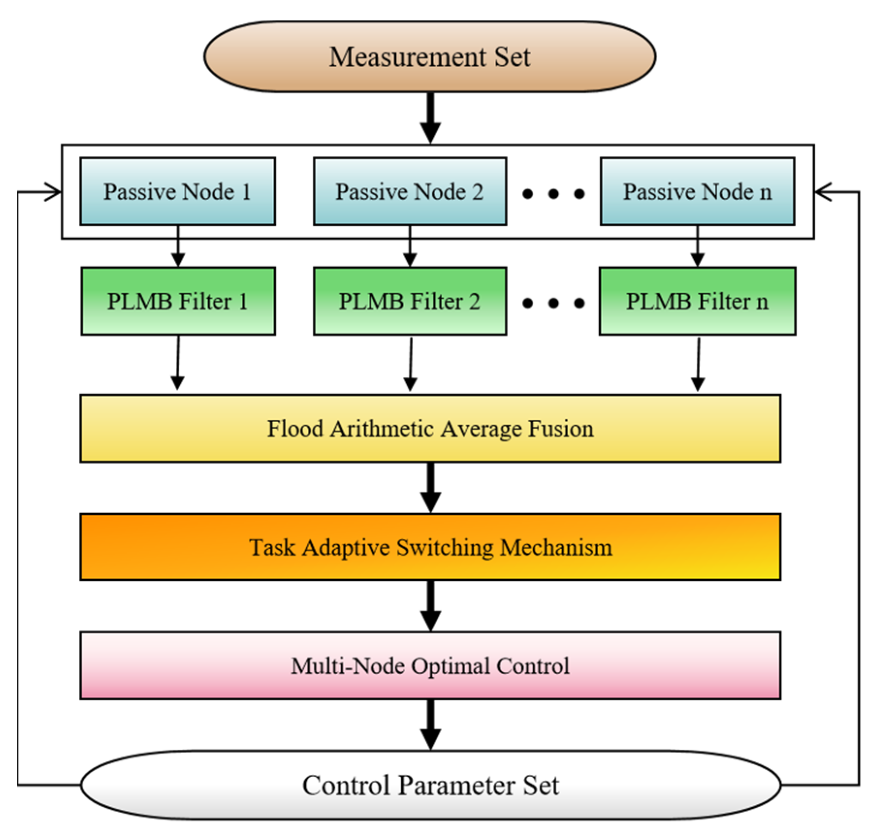
4. Multi-Node Joint Optimization Control Algorithm

Due to the limited FOV of the nodes and the stochastic nature of the appearance/disappearance of targets, the distributed APBR network needs to simultaneously search for undetected targets and track detected targets. In this paper, from the perspective of global optimization of the network, the search task and tracking task are decomposed so that all nodes execute only one task independently at any moment. In the network, a single node will perform task adaptive switching based on the local multi-target density to ensure that it performs optimization control based on the objective function of only one task. After completing the task adaptive switching, all nodes will be clustered according to the executed tasks, and nodes executing the same task will perform joint optimization control according to the objective function of the task, thus making the optimization result of a single task optimal and realizing the multi-target joint optimization control. In this way, the multi-objective optimization problem of the network is transformed into a single-objective optimization problem, which not only avoids the competition of detection resources between tasks but also improves the global optimization effect of the network. Next, the multi-node joint optimization control algorithm based on the task adaptive switching mechanism is given in this section.

4.1. Task Adaptive Switching Mechanism

The task adaptive switching means that each node automatically adapts the optimization task to be performed based on the target information within the FOV at the current moment and the global multi-target tracking situation of the network. To maximize the utilization of the detection resources of all nodes within the network, individual nodes must have the real-time switching capability of the tasks to be optimized. In this paper, each node can be defined according to the task type as S node and T node, and the corresponding set of nodes are denoted as $R_{\mathrm{S}}$ and $R_{\mathrm{T}}$. The S node is responsible for performing the target search task, and the task goal is to search the unknown region to detect more potential targets; T node is responsible for performing the target tracking task, and the task goal is to continuously track the detected targets. When the node performing the search task detects a target, it needs to stop searching and switch to performing the tracking task; when all targets within the FOV of the node performing the tracking task are dying out, the node needs to switch to performing the search task in time.

At the initial moment, the state, number, and distribution of targets in the network are unknown, and all sensor nodes are set as S nodes. For any S node, when the estimated number of targets within its FOV is greater than 0 for $m$ consecutive moments, its search task is switched to a tracking task and labeled as a T node. For any T node, when the number of targets in its FOV is estimated to be 0 for $m$ consecutive moments, its tracking task is switched to a searching task and labeled as an S node. $m$ is adjusted according to the detection probability of the receiver, and when the detection probability is larger, $m$ can be set smaller, on the contrary, when the detection probability is smaller, $m$ should be set larger.

In addition, assuming that the network multi-target tracking fusion error is set within the threshold range $\left[T{h}_{lower},T{h}_{upper}\right]$, when the network global multi-target tracking fusion error is higher than the upper bound of the threshold range, it indicates that the multi-target tracking fusion effect is poor and some of the S nodes should be switched to T nodes according to the principle of proximity to the target to perform the tracking task, so as to improve the tracking accuracy of the network to the detected target. When the global tracking fusion error of the network is lower than the upper bound of the threshold range, it indicates that the multi-target tracking fusion effect is better, and some of the T nodes can be switched to S nodes according to the overlap of the FOV coverage to improve the network’s search coverage of the undetected targets. In summary, all nodes in the network will adaptively switch the executed optimization control tasks in accordance with the designed task adaptive switching mechanism, combining their own state and the global multi-target tracking fusion results of the network.

4.2. Optimization Objective Function for Different Tasks

After the nodes in the network perform a fusion update of multi-target density, they need to estimate the target state and the number of targets at the same time, and the multi-target tracking performance will be affected by both the target state estimation and the number estimation. In view of this, the information entropy can be used in the optimal control algorithm to measure the information difference between the pseudo-predicted multi-target densities of the global fusion of the network and the pseudo-posteriori multi-target densities of the fusion of the different control schemes. In this way, the information difference of the multi-target densities can be measured directly, which can consider the effects of the target state estimation and the number estimation at the same time. Considering the computational complexity of the algorithm, this paper adopts differential entropy as the information difference measurement to derive the objective function for the target tracking task. In addition, the fusion intensity is used as the main measurement in the construction of the objective function for the target search task. Next, in this section, the objective functions in the search task and the tracking task are derived, respectively.

4.2.1. Derivation of the Objective Function for Tracking Tasks

The task-switching indicator function for T nodes is first constructed. The global multi-target tracking performance of the network is related to the PLMB density of the detected targets, and the LMB density part of the PLMB density reflects the tracking performance of the detected targets and the PDF of a single detected target can be expressed by the Gaussian component as the following:

$${\overline{p}}_{k+l}^{\mathcal{l}}\left(c_k\right){|}_{\mathcal{l}\in L_{k+l}}=\mathcal{N}\left(x;m_{k+l}^{\mathcal{l}}\left(c_k\right),P_{k+l}^{\mathcal{l}}\left(c_k\right)\right),$$

(37)

where $\left|L_{k+l}\right|$ reflects the estimation of the number of detected targets, and the covariance of the single-target PDF reflects the state estimation error of the detected targets. On this basis, this section uses the average tracking error function [37] of all detected targets as the task-switching indicator function of the T-node, for example, as follows:

$$D_{switch}=\frac{{\displaystyle \sum _{\mathcal{l}=1}^{\left|L_{k+l}\right|}tr\left(W{P}_{k+l}^{\mathcal{l}}\left(c_k\right)W\right)}}{\left|L_{k+l}\right|}.$$

(38)

where $\left|L_{k+l}\right|$ denotes the number of targets, $W$ denotes the extraction matrix of the position component in the covariance matrix $P_{k+l}^{\mathcal{l}}\left(c_k\right)$, and the multi-target average tracking error is taken to avoid the overall error becoming larger with the increase of the number of detected targets.

When $D_{switch}<T{h}_{lower}$, the multi-target tracking accuracy of the network is judged to be better, then some of the T nodes can be switched to S nodes to improve the network’s ability to search for undetected targets; the specific switching steps are as follows:

Step 1: Based on the respective tracking errors of the detected targets, find the label corresponding to the target with the smallest tracking error as follows:

$${\mathcal{l}}_{good}=\underset{\mathcal{l}}{\min } \mathrm{tr}\left(W{P}_k^{\mathcal{l}}{W}^{\mathrm{T}}\right),$$

(39)

Step 2: Extract the target position $m_k^{{\mathcal{l}}_{good}}$ corresponding to the label and find out all the T-nodes that have detected this target in the FOV and put them into the set $R_{\mathrm{T}/\mathrm{S}}$ of to-be-switched nodes. At the same time, to ensure that the estimation of the number of targets is not affected, T-nodes that contain other independent targets (which are only tracked by this T-node) in the FOV should be excluded from the set $R_{\mathrm{T}/\mathrm{S}}$.

Step 3: Based on the distance of this target from all the T-sensors in the set $R_{\mathrm{T}/\mathrm{S}}$, it is sorted according to the size of the distance. Considering that the farther the node is from the target, the larger the detection error is and the smaller the contribution to the target tracking performance. Switch the T node with the farthest distance in the set $R_{\mathrm{T}/\mathrm{S}}$ to an S node.

Next, the differential entropy is used to construct the optimal control cost function of T nodes. The differential entropy in the framework of RFS theory is defined as follows: for any RFS $X$, whose probability density is $f_X$, its corresponding differential entropy $h\left(X\right)$ is defined as the following:

$$h\left(X\right)=-{\mathbb{E}}_X\left[\ln f_X\right]=-{\displaystyle \int \ln \left(f_X\left(Y\right)\right)f_{\mathit{X}}\left(Y\right)\mu \left(dY\right)}.$$

(40)

$Y$ in Equation (39) denotes any finite subset of the RFS $X$ and $\mu$ is a reference measure defined as the following:

$$\mu \left(T\right)\triangleq {\displaystyle \sum _{i=0}^{\infty }\frac{1}{i!K^i}{\displaystyle \int 1_T(y_1,...,y_i)d(y_1,...,y_i)}}.$$

(41)

where $K$ is the hyper-volume unit on $X$, like the volume unit in the Euclidean space. $T$ is a finite subset of $X$, and $1_T\left(·\right)$ is the indicator function of $T$. Observing Equation (39), we can find that the differential entropy is essentially the negative logarithmic expectation of the probability density, which is used to measure the uncertainty of the RFS $X$, and the smaller the differential entropy, the smaller the uncertainty. The expectation ${\mathbb{E}}_X\left[\ln f_X\right]$ is obtained by taking the logarithm of the probability density $f_X$ and multiplying it by itself, and integrating over all possible subsets $Y$. Let $f_{X|Z}$ denote the conditional probability density of the RFS $X$ on $Z$, then based on Equation (39), can be expanded to obtain the definition of the conditional differential entropy as follows:

$$h(X\mid Z)=-{\mathbb{E}}_{X,Z}\left[\ln f_{X\mid Z}\right].$$

(42)

Further, let the multi-target density of the RFS $X$ be ${\mathit{\pi }}_X$, then the differential entropy of the multi-target density can be expressed using the definition of set integral aa follows:

$$h(\mathit{X})=-{\displaystyle \int \ln }\left(K^{\left|Y\right|}{\mathit{\pi }}_X(Y)\right){\mathit{\pi }}_X(Y)\delta Y.$$

(43)

Combining Equations (39) and (41) yields the mutual information between two RFSs $X$ and $Z$ can be expressed as follows:

$$I(\mathit{X};Z)=h(\mathit{X})-h(\mathit{X}\mid Z).$$

(44)

The mutual information in Equation (44) indicates the amount of information obtained by the RFS $X$ when acquiring the RFS $Z$, and the larger the mutual information, the smaller the uncertainty of $X$. Therefore, from the perspective of multi-target optimal control, the smaller the differential entropy of the multi-target state set or the larger the mutual information between the multi-target state set and the PIMS, the higher the accuracy of the multi-target trajectory estimation, and the T-node’s task is accomplished better. In this section, the LMB density part of the multi-target density at the time denotes the detected targets, denoted as ${\mathit{\pi }}_k^{LMB}\left(X\right)$. The optimal control of a T-node is essentially to solve for the optimal control scheme that minimizes the information difference between the multi-target predicted density ${\mathit{\pi }}_{k+l}^{LMB}\left(X\right)$ at time $k+l$ and the multi-target density ${\mathit{\pi }}_{k+l}^{LMB}\left(X|Z\left(c_k\right)\right)$ after the PIMS update. For an LMB density with a parameter set of ${\left\{r^{(\mathcal{l})},p^{(\mathcal{l})}(·)\right\}}_{\mathcal{l}\in \mathbb{L}}$, its differential entropy expression is as follows:

$$h(\mathit{X})=-{\displaystyle \sum _{\mathcal{l}\in \mathbb{L}}\left[r^{(\mathcal{l})}\ln r^{(\mathcal{l})}+{\tilde{r}}^{(\mathcal{l})}\ln {\tilde{r}}^{(\mathcal{l})}+r^{(\mathcal{l})}<p^{(\mathcal{l})},\ln \left(K{p}^{(\mathcal{l})}\right)>\right]}.$$

(45)

where ${\tilde{r}}^{(\mathcal{l})}=1-r^{(\mathcal{l})}$. Therefore, combining the multi-node optimal control model given in Equation (16) and the differential entropy definition of the LMB density in Equation (43), the optimal control function for all T nodes under the control scheme can be constructed as follows:

$$V_{track}\left(c_k\right)=-{\displaystyle \sum _{j=k+1}^{k+l}h\left({\mathit{X}}_j|Z_j\left(c_k\right)\right)}.$$

(46)

Equation (46) represents the cumulative differential entropy of the multi-target state given the PIMS in the control horizon $l$. To facilitate the calculation, Equation (46) is further disassembled as follows in conjunction with the definition of the PIMS value function in [37], as follows:

$$V_{track}(c_k)={\displaystyle \sum _{j=k+1}^{k+l}{\displaystyle \int \mathit{\varrho }}}\left(Z\left(c_k\right),X_j\right){\mathit{\pi }}_j^{lmb}\left(X_j\mid Z\left(c_k\right)\right)\delta X_j,$$

(47)

$$\mathit{\varrho }\left(Z\left(c_k\right),X_j\right)=\ln \left(K^{\left|\mathit{X}\right|}{\mathit{\pi }}_j^{lmb}(X_j\mid Z\left(c_k\right))\right).$$

(48)

In summary, Equations (38) and (46) are jointly constructed as the objective function in the tracking task, expressed as follows:

$${\theta }_{track}=\left[V_{track},D_{switch}\right].$$

(49)

The former represents the mutual information measurement function between the multi-target prediction density and the PIMS update density, which serves as the joint optimization control function of the T nodes in order to obtain more informative multi-target measurements; the latter represents the average tracking error function of all detected targets, which serves as the task-switching indicator function of the T nodes in order to better balance the allocation of the node’s detection resources in the network, and to improve the network’s potential undetected target search capability of the network.

4.2.2. Derivation of the Objective Function for Searching Tasks

The task-switching indicator function of S nodes is decided according to the global multi-target tracking performance of the network, and the task-switching indicator function given in Equation (38) is still used here; only the conditions of task-switching are different. When $D_{switch}>T{h}_{upper}$, the multi-target tracking performance of the network is judged to be poor, then some of the S nodes can be switched to T nodes to improve the tracking ability of the network on the detected targets; the specific switching steps are:

Step 1: Based on the global multi-target density of the network, extract the set of states of the detected targets at the current moment and find the target with the largest state estimation error, whose corresponding label is as follows:

$${\mathcal{l}}_{bad}=\underset{\mathcal{l}}{\max }\mathrm{tr}\left(W{P}_k^{\mathcal{l}}{W}^{\mathrm{T}}\right).$$

(50)

Step 2: Extract the location $m_k^{{\mathcal{l}}_{bad}}$ of the target corresponding to the label, calculate the distance from all S nodes to the target, and find the closest S node to the target as the to-be-switched node ${\mathrm{S}}_{\mathrm{T}}$ according to the proximity principle as follows:

$${\mathrm{S}}_{\mathrm{T}}=\underset{i\in R_S}{\min }\Vert m_k^{{\mathcal{l}}_{bad}}-m_k^i\Vert .$$

(51)

Step 3: If the target is located within the FOV of the node ${\mathrm{S}}_{\mathrm{T}}$, switch the node ${\mathrm{S}}_{\mathrm{T}}$ to T-node directly; if the target is located outside the FOV of the node ${\mathrm{S}}_{\mathrm{T}}$, control the node to move towards the target until the target enters the FOV of the node ${\mathrm{S}}_{\mathrm{T}}$, and then switch it to T-node.

Considering that the multi-target fusion density obtained by Equation (36) is the PLMB density, where the PPP part represents the intensity function of the undetected targets, integrating the PPP intensity function in the search area of the S node can get the expectation of the number of targets in the search area. Notice that the task-switching mechanism can ensure independence between the two tasks, and different methods can be chosen in the construction of the objective function according to the specific needs of the task. Therefore, to make the number of undetected targets in the network coverage area as small as possible, the objective function of the search task does not need to use the differential entropy construction method in the tracking task, and it can be directly integrated over the PPP intensity function in the coverage area of all S nodes as the optimization control function of the search task, for example, as follows:

$${\overline{D}}_{k+l}^U\left(c_k\right)={\displaystyle \sum _{j=1}^{J_k}{\alpha }_{k+l}^{U,j}}\left(c_k\right)\mathcal{N}\left(x;m_{k+l}^{U,j}\left(c_k\right),P_{k+l}^{U,j}\left(c_k\right)\right),$$

(52)

$$V_{search}\left(c_k\right)={\displaystyle \int {\overline{D}}_{k+l}^U\left(c_k\right)}={\displaystyle \sum _{j=1}^{J_k}{\alpha }_{k+l}^{U,j}}\left(c_k\right).$$

(53)

The objective function in the search task is constructed by combining Equations (38) and (53) and is expressed as follows:

$${\theta }_{search}=\left[V_{search},D_{switch}\right].$$

(54)

The former serves as an optimization control function for the intensity of undetected targets in the search region, which is used for the optimal control decision of multiple nodes under the search task to search more targets; the latter represents the average tracking error function of all detected targets, which measures the global multi-target tracking fusion effect of the network and serves as a task-switching indicator function for the S node, which is convenient for allocating more node probing resources to the target in the case of a poor tracking effect tracking to ensure the effectiveness of multi-target tracking fusion.

4.3. Joint Optimization Control Algorithm Flow

It is assumed that all the nodes in the network have completed the track initiation for the detected targets in the FOV and have completed the initial task allocation according to the targets in their respective FOVs. In the subsequent multi-target tracking fusion process of the network, all nodes will continue to execute the multi-node joint optimization control algorithm based on the task adaptive switching mechanism, and the specific implementation steps of the algorithm are as follows:

Step 1: All the nodes in the network execute local PLMB filters to obtain the multi-target density at time $k$ according to the multi-target measurement data obtained from their respective FOVs and perform AA fusion on the multi-target density based on the flooding communication strategy to obtain the global fusion multi-target posteriori density of the network. At the same time, the multi-target prediction density at time $k+l$ is calculated and the multi-target prediction state set at time $k+l$ is extracted.

Step 2: Extract the set of multi-target states at time $k$ and calculate $D_{switch}$. All nodes determine whether the global multi-target tracking accuracy of the network at the current moment is within the set threshold based on $D_{switch}$, and then perform task adaptive switching according to the determination result and the target situation within their respective FOVs. Finally, all nodes are clustered according to the task type.

Step 3: Firstly, according to the given set $C_k$ of control parameters, calculate the state set of each node under all control parameters, and calculate the PIMS received by each node under different control parameters according to the multi-target prediction state at time $k+l$, and then each node updates the multi-target posteriori density related to each control parameter based on the PIMS. Finally, AA fusion is performed on the multi-target posteriori densities of the same type’s nodes to obtain the fused multi-target posteriori density.

Step 4: Solve for the optimal set of control parameters for the T-nodes and S-nodes, respectively, according to the solution method of the single-objective optimization problem. For all T nodes, the control parameters are solved as follows:

$$c_k^{\mathrm{T}}=\underset{c_k\subset C_k}{arg\min }{V}_{track}\left(c_k\right).$$

(55)

For all S nodes, the control parameters are solved as follows:

$$c_k^{\mathrm{S}}=\underset{c_k\subset C_k}{arg\min }{V}_{search}\left(c_k\right).$$

(56)

Considering the intricate nature of the objective function and the stringent real-time constraints, a greedy algorithm is an optimal choice for solving the single-objective optimization problem. The specific details of this algorithm can be found [38]. The control parameters obtained by solving the two objective functions separately constitute the optimal control parameter set $c_k^{\mathrm{opt}}=c_k^{\mathrm{T}}\cup c_k^{\mathrm{S}}$ for multi-target joint optimization control at time $k$. Subsequently, all nodes adjust their motion heading in accordance with the optimal control parameter set $c_k^{\mathrm{opt}}$ and maneuver within the control FOV until the next control cycle commences.

For T nodes and S nodes, their numbers are denoted as $\left|R_{\mathrm{T}}\right|$ and $\left|R_{\mathrm{S}}\right|$, respectively, and the base of the alternative control parameter set is denoted as $\left|C_k\right|$, then the computational complexity of the algorithm can be expressed as $𝒪\left({\left|C_k\right|}^{\left|R_{\mathrm{T}}\right|}+{\left|C_k\right|}^{\left|R_{\mathrm{S}}\right|}\right)$. Because all nodes are clustered according to the task type in advance, and the single-objective optimization problem only needs to be solved independently according to the objective function corresponding to each task, the efficiency of the optimization solution will be greatly improved, and the optimal solution can be obtained in the process of solving the objective function under each task. The following section will present the results of a series of simulation experiments, the objective of which is to verify and analyze the practical effect of the proposed algorithm.

5. Simulation Verification and Result Analysis

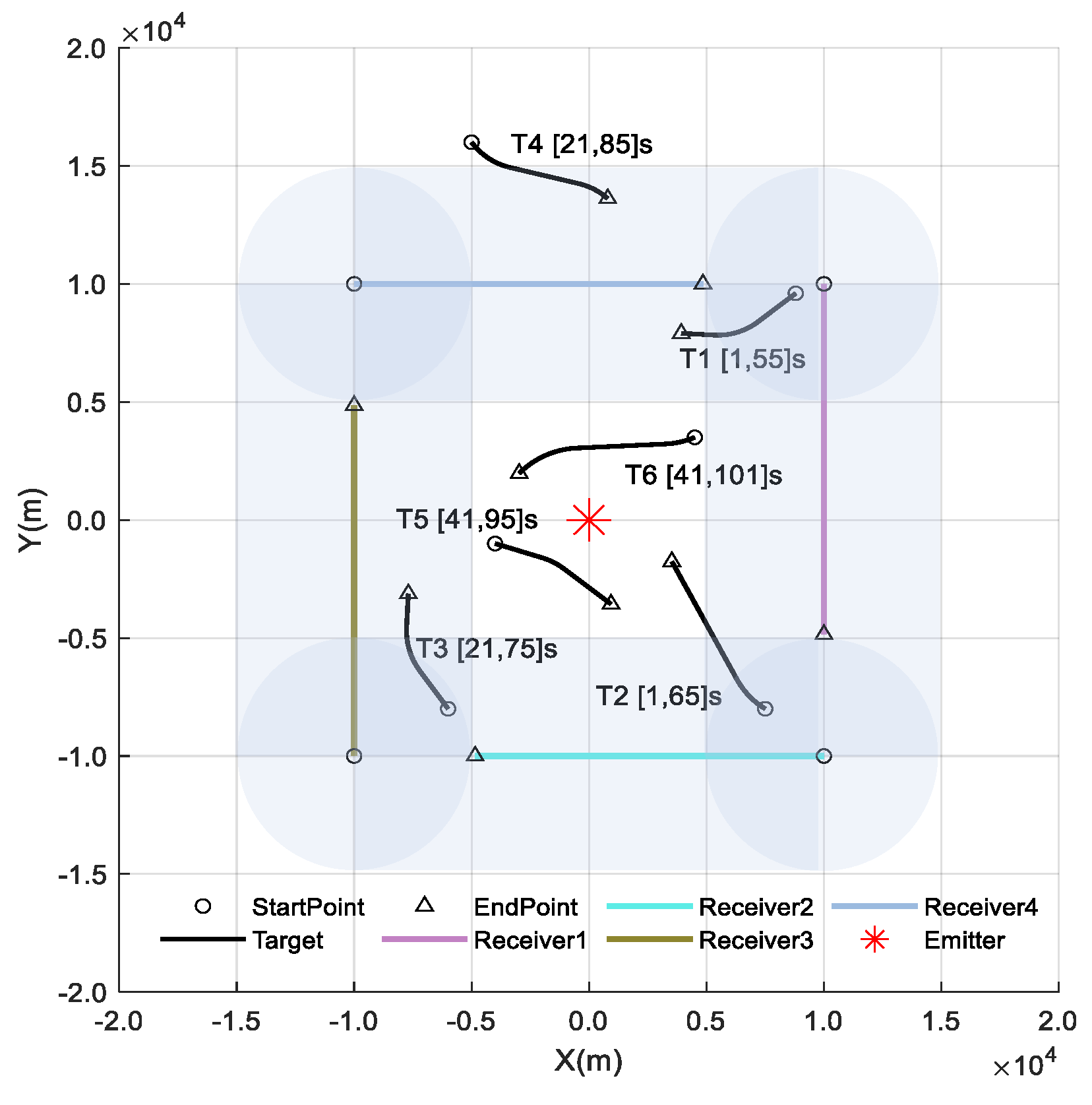
5.1. Experimental Scenario Setting

In this section, a multi-target tracking task scenario of a single-transmitter-multi-receiver distributed APBR network is designed to validate the effectiveness of the multi-node joint optimal control algorithm proposed in this paper in improving the multi-target tracking performance of the network. In the experiment, the whole range of the detection area is set as $\left[-20000,20000\right] \mathrm{m}\times \left[-20000,20000\right] \mathrm{m}$, and the center of the area is set with a fixed position of the non-cooperative emitter, the coordinates of which are $\left(0 \mathrm{m},0 \mathrm{m}\right),$ and its signal can cover the whole detection area. Considering the maneuverability of the UAV and the power coverage of the emitter, four UAVs equipped with passive sensors are dispersed in the detection area, constituting a distributed wireless sensor network, and each UAV can adjust its own state in real-time according to the control commands calculated by the algorithm. The detection period of the whole network is set to 100 s, and there are six targets appearing and disappearing at different moments during the detection period, and the altitude difference between the UAV and the targets is ignored. All the targets move in the CT model with an unknown turning rate, ${\omega }_k^{\mathcal{l}}$ is denoted as the turning rate of the target $\mathcal{l}$ at time $k$, and its state transfer equation is shown as follows:

$${\tilde{x}}_{+}^{\mathcal{l}}=F_{\mathrm{CT}}{\tilde{x}}_k^{\mathcal{l}}+W_k^{\mathcal{l}}$$

(57)

$${\mathit{F}}_{\mathrm{CT}}=\left[\begin{array}{cccc}1& 0& {\displaystyle \frac{sin\left({\omega }_k^{\ell }T\right)}{{\omega }_k^{\ell }}}& {\displaystyle \frac{cos\left({\omega }_k^{\ell }T\right)-1}{{\omega }_k^{\ell }}}\\ 0& 1& {\displaystyle \frac{1-cos\left({\omega }_k^{\ell }T\right)}{{\omega }_k^{\ell }}}& {\displaystyle \frac{1-cos\left({\omega }_k^{\ell }T\right)}{{\omega }_k^{\ell }}}\\ 0& 0& cos\left({\omega }_k^{\ell }T\right)& -sin\left({\omega }_k^{\ell }T\right)\\ 0& 0& sin\left({\omega }_k^{\ell }T\right)& cos\left({\omega }_k^{\ell }T\right)\end{array}\right]$$

(58)

$$W_k^{\mathcal{l}}=\left[n_p,n_p,n_v,n_v\right]$$

(59)

where $W_k^{\mathcal{l}}$ denotes the additive Gaussian process noise, $n_p~\mathcal{N}\left(0,{\sigma }_p^2\right)$, $n_v~\mathcal{N}\left(0,{\sigma }_v^2\right)$, ${\sigma }_p=0.5{\sigma }_a·T^2$ and ${\sigma }_v={\sigma }_a·T$ denotes the standard deviation of the process noise for position and velocity, ${\sigma }_a=1 {\mathrm{m}/\mathrm{s}}^2$ denotes the standard deviation of the acceleration noise and $T=1 \mathrm{s}$ is the sampling interval of the receiver. The initial state of the target and the moment of birth and death, as well as the initial state settings of each UAV in the APBR network, are shown in

Table 1. Initial state settings of simulated entities in the detection area.

Simulated Entity	$\mathbf{Initial}\mathbf{State}\left[\mathit{x}\mathbf{m};\dot{\mathit{x}}\mathbf{m}/\mathbf{s};\mathit{y}\mathbf{m};\dot{\mathit{y}}\mathbf{m}/\mathbf{s}\right]$	$\mathbf{Survival}\mathbf{Duration}\left[{\mathit{t}}_{\mathit{b}}/\mathbf{s},{\mathit{t}}_{\mathit{d}}/\mathit{s}\right]$
Target 1	[8800; −80; 9600; −60]	[1, 55]
Target 2	[7500; −100; −8000; 60]	[1, 65]
Target 3	[−6000; −60; −8000; 80]	[21, 75]
Target 4	[−5000; 60; 16,000; −80]	[21, 85]
Target 5	[−4000; 100; −1000; −30]	[41, 95]
Target 6	[4500; −120; 3500; −50]	[41, 101]
Emitter	[0; 0; 0; 0]	-
Receiver 1	[10,000; 0; 10,000; −150]	-
Receiver 2	[10,000; −150; −10,000; 0]	-
Receiver 3	[−10,000; 0; −10,000; 150]	-
Receiver 4	[−10,000; 150; 10,000; 0]	-

.

The target measure received by the UAV is a nonlinear measure combination consisting of DOA-TDOA-FDOA; the measurement model has been given in Section 2.2, described by Formulas (7)–(11), and the measurement noise is set to the following:

$$V_k=\left[n_{{\theta }_{\mathcal{l}}},n_{{\theta }_s}{n}_{td},n_{fd}\right],$$

(60)

where $n_{{\theta }_{\mathcal{l}}}~\mathcal{N}\left(0,{\sigma }_{{\theta }_{\mathcal{l}}}^2\right)$, $n_{{\theta }_{\mathcal{l}}}~\mathcal{N}\left(0,{\sigma }_{{\theta }_s}^2\right)$, $n_{td}~\mathcal{N}\left(0,{\sigma }_{td}^2\right)$, $n_{fd}~\mathcal{N}\left(0,{\sigma }_{fd}^2\right)$ are measurement noise distribution for target arrival angle, emitter arrival angle, bistatic range, and bistatic range rate, respectively. ${\sigma }_{{\theta }_{\mathcal{l}}}={\sigma }_{{\theta }_s}=0.05 \mathrm{rad}$, σ_td = 100 m, ${\sigma }_{fd}=2 \mathrm{m}/\mathrm{s}$ denote the standard deviation of the measurement noise, respectively.

It is assumed that all clutter in the measurement data set received by each UAV node are uniformly distributed in the detection area, and the number of clusters at each sampling moment obeys a Poisson distribution with the parameter ${\lambda }_C$. The detection FOV of all UAV nodes in the network is set to be a circular area of radius $R_{\mathrm{FOV}}$, and the probability of detecting a target inside the FOV is $P_D$, and the probability of detecting a target outside the FOV is 0. The basic parameters of the UAV nodes are set, as shown in

Table 2. Basic parameter settings of the drone node.

Simulation Parameters	Specific Values
Detection radius of the node FOV $R_{\mathrm{FOV}}$	5000 m
Probability of detection within node FOV $P_D$	0.95
Target Track Confirmation Time $m$	3
$\mathrm{clutter}\mathrm{rate}{\lambda }_C$	5
$\mathrm{Target}\mathrm{survival}\mathrm{probability}{P}_S$	0.99
Target Extraction Threshold	0.5
$\mathrm{GM}\mathrm{pruning}\mathrm{threshold}T{h}_{\mathrm{GMp}}$	10−5
GM merging threshold ThGMm	10
Survival probability of newborn BCs $E{P}_n$	0.01
$\mathrm{BCs}\mathrm{pruning}\mathrm{threshold}T{h}_{prune}$	10−5
$\mathrm{BCs}\mathrm{merging}\mathrm{threshold}T{h}_{\mathrm{Merge}}$	30

.

Under the same experimental parameter settings, this paper will give the multi-target tracking performance when using only the multi-node fusion algorithm and compare the multi-target tracking performance when using the multi-node joint optimization control algorithm proposed in this paper and the multi-task joint optimization algorithm proposed in [39], to validate the necessity and the effectiveness of the proposed multi-target joint optimization control algorithm. The algorithm performance comparison metrics are chosen to be Generalized Optimal Sub-pattern Assignment (GOSPA) [40] and OSPA⁽²⁾ [41] with the truncation parameter set to $c=200$, the order set to $p=2$, and the window length set to $L=10$. The Monte Carlo count is set to 200. The cruising speed of the UAV nodes is set to $v_s=150 \mathrm{m}/\mathrm{s}.$ It is assumed that all the UAV nodes to be optimally controlled hover at the initial position and move at a constant cruising speed according to the initial heading after receiving the detection command. When all the UAV nodes in the network execute the joint optimization control algorithm, the control FOV length is set to $l=10 \mathrm{s}$, and the range of the alternative heading angle control parameters of the UAV is set to $C_k^i=\left[-180°,-179°,\cdots ,0°,\cdots ,179°,180°\right]$. That is, during the whole detection cycle of the APBR network, all UAV nodes carry out mission adaptive switching every 10 s and adjust the heading according to the control command parameters given by the joint optimization control algorithm before executing the next stage of the mission.

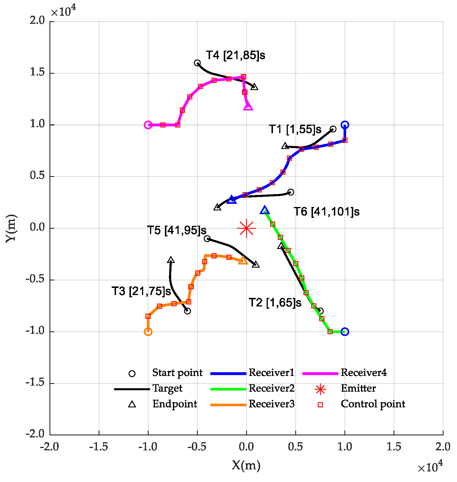
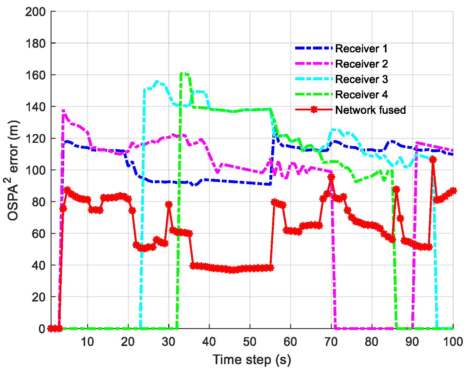
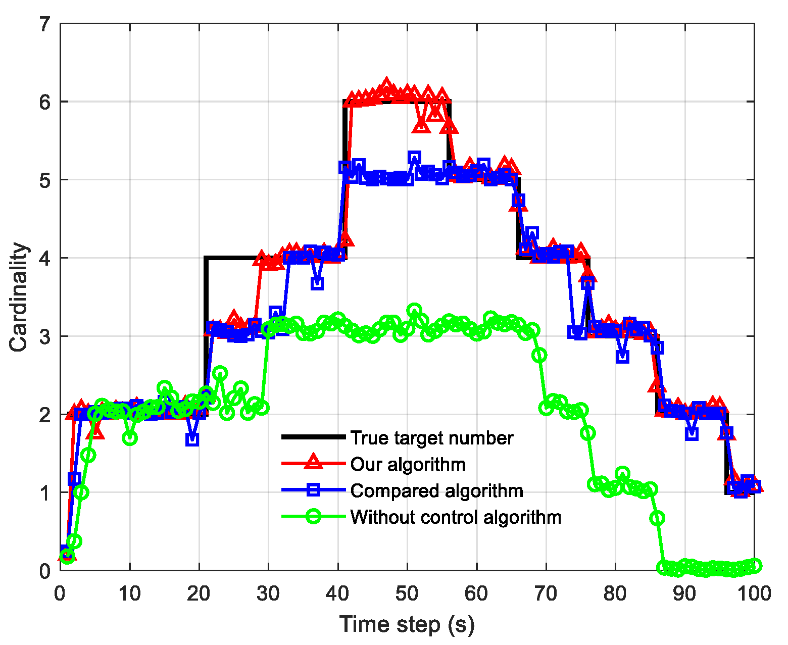
5.2. Analysis of Experimental Results

First, Figure 3 gives the multi-target tracking scene of the simulation experiment. Each node sets the heading at the initial moment to be clockwise coordinated uniform motion, keeping the same distance from each other, and the patrol tracks set by all the nodes when no control algorithm is used are shown in Figure 3. In Figure 3, all the target tracks are described by the start point ○ and the endpoint Δ, as well as the duration of the tracks, and the shaded portion indicates the area that can be covered by all the nodes when detecting the targets according to the set patrol routes. The nodes are symmetrically distributed around the emitter, and the sum of the FOVs of all nodes cannot cover the entire detection area of interest. In the scene, target 1 and target 2 are in the FOV of the nodes just after birth, target 4 enters the FOV of the nodes sometime after birth, and target 5 and target 6 do not enter the FOV of any of the nodes during the whole detection duration. If the UAV nodes patrol according to the set route, it will inevitably lead to target 5 and target 6 never being detected, and the tracking tracks of some of the targets will also be incomplete.

Figure 4 gives a graph of the motion tracks formed by each node under the command control of the multi-node joint optimization control algorithm proposed in this paper. The motion tracks of each node are described by the start point ○, the control point □, and the endpoint Δ. Since the length of the control, FOV is 10 s, every 10 s, the node carries out the execution of a task-switching decision and makes a control command decision based on the task type to determine the heading angle in the next control cycle.

Table 3. Task execution of multiple nodes at different control moments.

Control Moments/s	Receiver 1	Receiver 2	Receiver 3	Receiver 4
1	S	S	S	S
11	T	T	S	S
21	T	T	T	S
31	T	T	T	T
41	T	T	T	T
51	T	T	T	T
61	T	T	T	T
71	T	T	T	T
81	T	T	T	T
91	T	T	T	S

gives the task assignments for each node at each control point. Combining Figure 4 and Table 3, target 1 and target 2 appeared in the 1st control moment, but at that moment k < m, the nodes were unable to confirm the target track, so all nodes performed the search task. In the 2nd control moment, targets 1 and 2 are detected by node 1 and node 2, respectively, while no target is detected in node 3 and node 4, which continue to perform the search task. In the 3rd control moment, target 3 and target 4 are born; target 3 is detected by node 3, but target 4 has not been detected yet, so node 3 switches to perform the tracking task, and node 4 continues to search in the direction of target 4. At the 4th control moment, target 4 is detected, and node 4 switches to tracking target 4. At the 5th control moment, target 5 and target 6 are born but not yet detected. At the 6th control moment, all nodes were performing the tracking task, and nodes 1 and node 3 were tracking two targets at the same time because target 5 and target 6 had entered the FOV of node 1 and node 3, respectively. In the 7th control moment, target 1 disappeared, resulting in only target 6 existing within the FOV of node 1, so node 1 continued to track target 6. In the 8th control moment, target 2 disappeared, and target 5 entered the FOV of node 2, so node 2 continued to perform the tracking task. In the 9th control moment, target 3 disappeared, and only target 5 exists within the FOV of node 3, so node 3 continues to track target 5. In the 10th control moment, target 4 has disappeared, and node 4 switches to the searching task, but since there is no undetected target in the scene, node 4 searches in the direction of the nearest target 6; at the same time, node 2 switches to the T-node to track target 6 according to the proximity principle.

Figure 5 gives the GOSPA error plots of the local filtering results of each node and the global fusion results of the APBR network. From the localization error given in Figure 5a, when there is no target in the node’s FOV, the localization error is 0. When there is a target in the node’s FOV, the target localization error will gradually decrease with the optimization of the control algorithm. Specifically, in the first 20 s, only target 1 and target 2 appear, node 1 and node 2 perform the tracking task, and the localization error of the node’s local filter gradually decreases during the execution of the control command moving towards the tracked target. Between 21–30 s, node 3 tracks target 3, but node 4 has not yet tracked target 4, causing the network global fusion localization error to increase further. Between 31–40 s, node 4 tracked target 4, and the localization error gradually decreased during the control process. Between 41–70 s, all nodes perform the tracking task; the localization error is relatively stable and only becomes larger when the number of targets changes. Between 71–95 s, the number of targets changes frequently, and the localization error varies greatly. In the last 5 s, all the detection nodes are used to track target 6, which decreases the target localization error. The false alarm error in Figure 5b is lower throughout the detection period because the probability of detecting clutter is small due to the low clutter density setting and limited node FOV in the scene, so there is almost no target false alarm at each node. Figure 5c reflects the target missing from each node; due to the limited node FOV, each node detects a limited number of targets, the missing is obvious, and the error is large; while the global target missing from the network is relatively good, only in the detection area when the number of targets changes there will be a delay in detection time, resulting in an increase in the missing error at some moments, indicating that the adopted flooding communication strategy and AA fusion criteria are more effective and can effectively fuse the target information of each node. From the GOSPA error given in Figure 5d, as the number of nodes involved in tracking increases, the GOSPA error of the fusion result decreases gradually and is always smaller than the GOSPA error of the local filters of each node. In addition, the main sources of the GOSPA error are still the target localization error and the missing error, which is more obvious in the change curve of the GOSPA error of the fusion result.

Figure 6 gives the OSPA⁽²⁾ error map of the local filtering results of each node and the fusion results of the APBR network when using the multi-node joint optimal control algorithm, which is used to reflect the multi-target track estimation by each node and the APBR network, and to validate the effect of the algorithm proposed in this paper on the estimation of multi-target tracks when the nodes’ FOV is limited. From Figure 6, the error variation rule of OSPA⁽²⁾ is close to the GOSPA error in Figure 5, which indicates that the main sources of the error of OSPA⁽²⁾ are the target state estimation error and the target number estimation error, and the error caused by the interruption of the trajectory is smaller. The PLMB filter used in this paper can estimate the target tracks with good track continuity.

The GOSPA error comparison plot of the global fusion results of the APBR network under different algorithms is given in Figure 7, which is used to evaluate the necessity and effectiveness of using a multi-node joint optimization control algorithm. Since the multi-task joint optimization algorithm in [38] uses a PMBM filter and does not estimate the target tracks, the comparison of the OSPA⁽²⁾ error is not performed in this paper. From Figure 7, it can be clearly seen that the GOSPA error has been higher when the multi-target joint optimization control algorithm is not used; the reason is that the FOV of each node in the APBR network is limited, and it cannot detect all the targets in the area, there is a serious target missing, and the effect of the target tracking is not satisfactory. The patterns of change in GOSPA error of the multi-task joint optimization algorithm in [39] is close to the algorithm proposed in this paper, but the error value is higher than the algorithm proposed in this paper overall. The reason is that the multi-task joint optimization algorithm adopts a weighted method to allocate the detection resources of the sensor nodes, especially when the number of targets changes. The allocation of detection resources will be unreasonable, resulting in an increase in the error. In addition, the complexity of the algorithm in multi-task joint optimization is high, the computation is large, and the optimization control of each node will not be timely. In contrast, the tracking task objective function used in the algorithm proposed in this paper is more reasonable, and the target localization error will be smaller. In addition, the use of a task adaptive switching mechanism can allocate the detection resources of sensor nodes more reasonably, and the control response to each node is more rapid when the number of targets changes.

The target number estimation results of the global fusion results of the APBR network under different algorithms are given in Figure 8, which is used to compare and verify the accuracy of the target number estimation in the detection area using the joint multi-target optimization control algorithm. From Figure 8, the target number estimation when the control algorithm is not used is poor due to the limited node FOV. This is because even if the multi-target information is fused interactively, there will be some targets that are not within the FOV of all the nodes, and these targets are bound to miss detection. The multi-task joint optimization algorithm proposed in [39] can estimate all the targets appearing in the detection area, but the delay in estimating the number of targets in the network fusion result is large when the number of targets varies since the target search task and the tracking task are performed simultaneously. This is because the weighting method used in the algorithm cannot reasonably allocate the detection resources of the sensor nodes, especially when the number of targets changes. The allocation of detection resources will be more unreasonable, resulting in the target number estimation error becoming larger. In contrast, the multi-node joint optimization control algorithm proposed in this paper is based on the task adaptive switching mechanism, and all nodes are reclassified according to different tasks, which transforms the multi-task optimization problem into a single-task optimization problem. Therefore, the proposed algorithm can not only reasonably allocate the detection resources of the sensor nodes but also reduce the complexity of the algorithm, improve the optimization and control efficiency, and estimate the number of targets in the detection area more accurately.

6. Conclusions

This paper introduces a multi-node joint optimal control algorithm for addressing the multi-target tracking challenge in distributed APBR networks, focusing on incomplete target detection due to limited node FOV. Initially, a PLMB filter is applied at each network node to capture local multi-target density within their respective FOVs. Subsequently, the AA fusion rule, utilizing a flooding strategy, integrates multi-target densities from various sensor nodes. To tackle incomplete target detection resulting from limited FOVs, a task-adaptive switching mechanism classifies sensor nodes into search and tracking nodes, simplifying the optimization problem. Objective functions for tracking and searching tasks are derived based on differential entropy and intensity functions. The GM-CKF method facilitates joint optimal control for multi-sensor nodes by implementing local filtering and density fusion. The greedy algorithm resolves single-task optimization, enhancing multi-target tracking and fusion efficiency. Simulation results show real-time optimal control capability and efficient sensor resource allocation. This algorithm proves crucial for overcoming incomplete target detection and improving distributed APBR network performance. Future studies will incorporate factors like signal resources, network loads, and sensor power consumption to enhance the network’s utility in complex electromagnetic environments.

References

1. Hu, S.; Yi, J.; Wan, X.; Cheng, F.; Hu, Y.; Hao, C. Illuminator of Opportunity Localization for Digital Broadcast-Based Passive Radar in Moving Platforms. IEEE Trans. Aerosp. Electron. Syst. 2023, 59, 3539–3549. [Google Scholar] [CrossRef]
2. Gabard, B.; Wasik, V.; Rabaste, O.; Deloues, T.; Poullin, D.; Jeuland, H. Airborne Targets Detection by UAV-Embedded Passive Radar. In Proceedings of the 2020 17th European Radar Conference (EuRAD), Utrecht, The Netherlands, 10–15 January 2021; pp. 346–349. [Google Scholar]
3. Malanowski, M.; Rytel-Andrianik, R.; Kulpa, K.; Stasiak, K.; Ciesielski, M.; Kulpa, J. Geometric Clutter Analysis for Airborne Passive Coherent Location Radar. IEEE Trans. Geosci. Remote Sens. 2022, 60, 1–14. [Google Scholar] [CrossRef]
4. Zhao, Z.; Cao, Y.; Wang, Y.; Zhou, H. Transmitted-Signal-Free Target Information Extraction for OFDM-Based Passive Radar with Time-Varying Sparse Model. IEEE Geosci. Remote Sens. Lett. 2023, 20, 1–5. [Google Scholar] [CrossRef]
5. Colone, F.; Filippini, F.; Pastina, D. Passive Radar: Past, Present, and Future Challenges. IEEE Aerosp. Electron. Syst. Mag. 2023, 38, 54–69. [Google Scholar] [CrossRef]
6. Sun, Z.; Wu, J.; Yen, G.G.; Lu, Z.; Yang, J. Performance Analysis and System Implementation for Energy-Efficient Passive UAV Radar Imaging System. IEEE Trans. Veh. Technol. 2023, 72, 9938–9955. [Google Scholar] [CrossRef]
7. Mahler, R.P.S. Multitarget Bayes filtering via first-order multitarget moments. IEEE Trans. Aerosp. Electron. Syst. 2003, 39, 1152–1178. [Google Scholar] [CrossRef]
8. Vo, B.; Vo, B.; Cantoni, A. Bayesian Filtering with Random Finite Set Observations. IEEE Trans. Signal Process. 2008, 56, 1313–1326. [Google Scholar] [CrossRef]
9. Saucan, A.; Coates, M.J.; Rabbat, M. A Multisensor Multi-Bernoulli Filter. IEEE Trans. Signal Process. 2017, 65, 5495–5509. [Google Scholar] [CrossRef]
10. García-Fernández, Á.F.; Williams, J.L.; Granström, K.; Svensson, L. Poisson Multi-Bernoulli Mixture Filter: Direct Derivation and Implementation. IEEE Trans. Aerosp. Electron. Syst. 2018, 54, 1883–1901. [Google Scholar] [CrossRef]
11. Boström-Rost, P.; Axehill, D.; Hendeby, G. Sensor Management for Search and Track Using the Poisson Multi-Bernoulli Mixture Filter. IEEE Trans. Aerosp. Electron. Syst. 2021, 57, 2771–2783. [Google Scholar] [CrossRef]
12. Vo, B.; Vo, B.; Phung, D. Labeled Random Finite Sets and the Bayes Multi-Target Tracking Filter. IEEE Trans. Signal Process. 2014, 62, 6554–6567. [Google Scholar] [CrossRef]
13. Reuter, S.; Vo, B.; Vo, B.; Dietmayer, K. The Labeled Multi-Bernoulli Filter. IEEE Trans. Signal Process. 2014, 62, 3246–3260. [Google Scholar] [CrossRef]
14. Vo, B.; Vo, B.; Hoang, H.G. An Efficient Implementation of the Generalized Labeled Multi-Bernoulli Filter. IEEE Trans. Signal Process. 2017, 65, 1975–1987. [Google Scholar] [CrossRef]
15. Cament, L.; Correa, J.; Adams, M.; Pérez, C. The histogram Poisson, labeled multi-Bernoulli multi-target tracking filter. Signal Process. 2020, 176, 107714–107729. [Google Scholar] [CrossRef]
16. Li, G.; Battistelli, G.; Yi, W.; Kong, L. Distributed multi-sensor multi-view fusion based on generalized covariance intersection. Signal Process. 2020, 166, 107246. [Google Scholar] [CrossRef]
17. Li, G.; Battistelli, G.; Chisci, L.; Gao, L.; Wei, P. Distributed Joint Detection, Tracking, and Classification via Labeled Multi-Bernoulli Filtering. IEEE Trans. Cybern. 2024, 54, 1429–1441. [Google Scholar] [CrossRef]
18. Shen, K.; Dong, P.; Jing, Z.; Leung, H. Consensus-Based Labeled Multi-Bernoulli Filter for Multitarget Tracking in Distributed Sensor Network. IEEE Trans. Cybern. 2022, 52, 12722–12733. [Google Scholar] [CrossRef]
19. Yi, W.; Li, G.; Battistelli, G. Distributed Multi-Sensor Fusion of PHD Filters with Different Sensor Fields of View. IEEE Trans. Signal Process. 2020, 68, 5204–5218. [Google Scholar] [CrossRef]
20. Li, T.C.; Song, Y.; Song, E.B.; Fan, H.Q. Arithmetic average density fusion—Part I: Some statistic and information-theoretic results. Inf. Fusion 2024, 104, 102199. [Google Scholar] [CrossRef]
21. Li, T. Arithmetic Average Density Fusion—Part II: Unified Derivation for Unlabeled and Labeled RFS Fusion. IEEE Trans. Aerosp. Electron. Syst. 2024, 60, 3255–3268. [Google Scholar] [CrossRef]
22. Li, T.; Yan, R.; Da, K.; Fan, H. Arithmetic Average Density Fusion—Part III: Heterogeneous Unlabeled and Labeled RFS Filter Fusion. IEEE Trans. Aerosp. Electron. Syst. 2024, 60, 1023–1034. [Google Scholar] [CrossRef]
23. Li, T.C.; Hlawatsch, F. A distributed particle-PHD filter using arithmetic-average fusion of Gaussian mixture parameters. Inf. Fusion 2021, 73, 111–124. [Google Scholar] [CrossRef]
24. Battistelli, G.; Chisci, L.; Fantacci, C.; Farina, A.; Graziano, A. Distributed multitarget tracking for passive multireceiver radar systems. In Proceedings of the 2013 14th International Radar Symposium (IRS), Dresden, Germany, 19–21 June 2013; pp. 337–342. [Google Scholar]
25. Li, S.; Yi, W.; Hoseinnezhad, R.; Battistelli, G.; Wang, B.; Kong, L. Robust Distributed Fusion with Labeled Random Finite Sets. IEEE Trans. Signal Process. 2018, 66, 278–293. [Google Scholar] [CrossRef]
26. Li, S.; Battistelli, G.; Chisci, L.; Yi, W.; Wang, B.; Kong, L. Computationally Efficient Multi-Agent Multi-Object Tracking with Labeled Random Finite Sets. IEEE Trans. Signal Process. 2019, 67, 260–275. [Google Scholar] [CrossRef]
27. Gostar, A.K.; Hoseinnezhad, R.; Bab-Hadiashar, A. Multi-bernoulli sensor control via minimization of expected estimation errors. IEEE Trans. Aerosp. Electron. Syst. 2015, 51, 1762–1773. [Google Scholar] [CrossRef]
28. Gostar, A.K.; Hoseinnezhad, R.; Bab-Hadiashar, A.; Liu, W. Sensor-Management for Multitarget Filters via Minimization of Posterior Dispersion. IEEE Trans. Aerosp. Electron. Syst. 2017, 53, 2877–2884. [Google Scholar] [CrossRef]
29. Ristic, B.; Vo, B.; Clark, D. A Note on the Reward Function for PHD Filters with Sensor Control. IEEE Trans. Aerosp. Electron. Syst. 2011, 47, 1521–1529. [Google Scholar] [CrossRef]
30. Beard, M.; Vo, B.T.; Vo, B.N.; Arulampalam, S. Sensor control for multi-target tracking using Cauchy-Schwarz divergence. In Proceedings of the 2015 18th International Conference on Information Fusion (Fusion), Washington, DC, USA, 6–9 July 2015; pp. 937–944. [Google Scholar]
31. Zhu, Y.; Liang, S.; Gong, M.; Yan, J. Decomposed POMDP Optimization-Based Sensor Management for Multi-Target Tracking in Passive Multi-Sensor Systems. IEEE Sens. J. 2022, 22, 3565–3578. [Google Scholar] [CrossRef]
32. LeGrand, K.A.; Zhu, P.; Ferrari, S. A Random Finite Set Sensor Control Approach for Vision-based Multi-object Search-While-Tracking. In Proceedings of the 2021 IEEE 24th International Conference on Information Fusion (FUSION), Sun City, South Africa, 1–4 November 2021; pp. 1–8. [Google Scholar]
33. Nguyen, H.V.; Vo, B.N.; Vo, B.T.; Rezatofighi, H.; Ranasinghe, D.C. Multi-Objective Multi-Agent Planning for Discovering and Tracking Multiple Mobile Objects. IEEE Trans. Signal Process. 2024, 72, 3669–3685. [Google Scholar] [CrossRef]
34. Li, T.; Corchado, J.M.; Prieto, J. Convergence of Distributed Flooding and Its Application for Distributed Bayesian Filtering. IEEE Trans. Signal Inf. Process. Netw. 2017, 3, 580–591. [Google Scholar] [CrossRef]
35. Chen, X.; Tharmarasa, R.; Pelletier, M.; Kirubarajan, T. Integrated Clutter Estimation and Target Tracking Using Poisson Point Processes. IEEE Trans. Aerosp. Electron. Syst. 2012, 48, 1210–1235. [Google Scholar] [CrossRef]
36. Wei, J.; Luo, F.; Qi, J.; Luo, X. Distributed Fusion of Labeled Multi-Bernoulli Filters Based on Arithmetic Average. IEEE Signal Process. Lett. 2024, 31, 656–660. [Google Scholar] [CrossRef]
37. Boström-Rost, P.; Axehill, D.; Hendeby, G. PMBM Filter with Partially Grid-Based Birth Model with Applications in Sensor Management. IEEE Trans. Aerosp. Electron. Syst. 2022, 58, 530–540. [Google Scholar] [CrossRef]
38. Verma, J.K.; Chhabra, J.K.; Ranga, V. Track Consensus-Based Labeled Multi-Target Tracking in Mobile Distributed Sensor Network. IEEE Trans. Mob. Comput. 2024, 23, 7351–7362. [Google Scholar] [CrossRef]
39. Chen, K.; Chai, L.; Yi, W. Multi-Sensor Control for Jointly Searching and Tracking Multi-Target Using the Poisson Multi-Bernoulli Mixture Filter. In Proceedings of the 2022 11th International Conference on Control, Automation and Information Sciences (ICCAIS), Hanoi, Vietnam, 21–24 November 2022; pp. 240–247. [Google Scholar]
40. Rahmathullah, A.S.; García-Fernández, Á.F.; Svensson, L. Generalized optimal sub-pattern assignment metric. In Proceedings of the 2017 20th International Conference on Information Fusion (Fusion), Xi’an, China, 10–13 July 2017. [Google Scholar]
41. Beard, M.; Vo, B.T.; Vo, B.N. OSPA(2): Using the OSPA metric to evaluate multi-target tracking performance. In Proceedings of the 2017 International Conference on Control, Automation and Information Sciences (ICCAIS), Chiang Mai, Thailand, 31 October–1 November 2017; pp. 86–91. [Google Scholar]
Figure 1. An overview of the research core.
Drones 08 00627 g001
Figure 2. Passive Multi-node Joint Optimization Control Flow.
Drones 08 00627 g002
Figure 3. Scenario diagram of multi-target tracking simulation.
Drones 08 00627 g003
Figure 4. Motion tracks of each node under control commands.
Drones 08 00627 g004
Figure 5. GOSPA error profile of local filtering results and fusion results.
Drones 08 00627 g005
Figure 6. OSPA(2) error plot for local filtering results and fusion results.
Drones 08 00627 g006
Figure 7. Comparison of GOSPA errors of fusion results under different algorithms.
Drones 08 00627 g007
Figure 8. Estimated target number of fusion results under different algorithms.
Drones 08 00627 g008