
Fault-Tolerant Event-Triggrred Control for Multiple UAVs with Predefined Tracking Performance


Abstract
1. Introduction
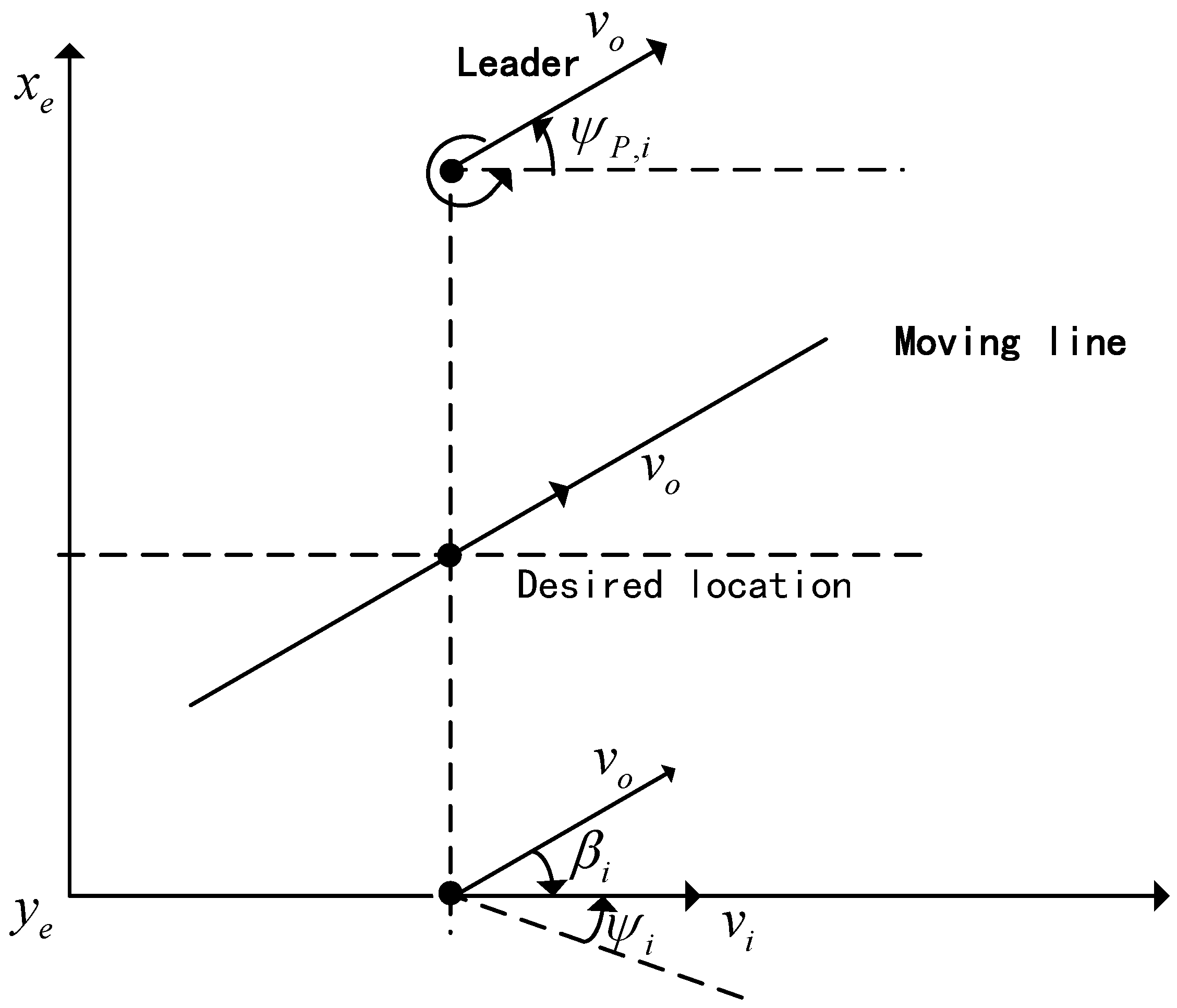
- The guidance rate of formation control is designed using a line-of-sight (LOS) guidance algorithm, and the performance of the formation-tracking error is realized using a Lyapunov function. This approach is compared with the method proposed in [36], and it provides better performance by bounding the convergence error.
- A sampling adaptive tracking controller is proposed for the velocity and yaw angle loop, in combination with the radial basis function neural network (RBFNN). This approach performs better in case of actuator failure and external disturbances, with a reduction in communication and actuation consumption compared to the work presented in [38].
- A novelty sampling mode with an event-triggering mechanism is designed, which utilizes only the input information to implement the sampling. This approach avoids the need for dedicated monitoring devices, as seen in the triggering mode presented in [29], and reduces the communication burden of the actuation.
2. Problem Statement
2.1. Dynamic Modeling of the Multiple Non-Linear UAVs
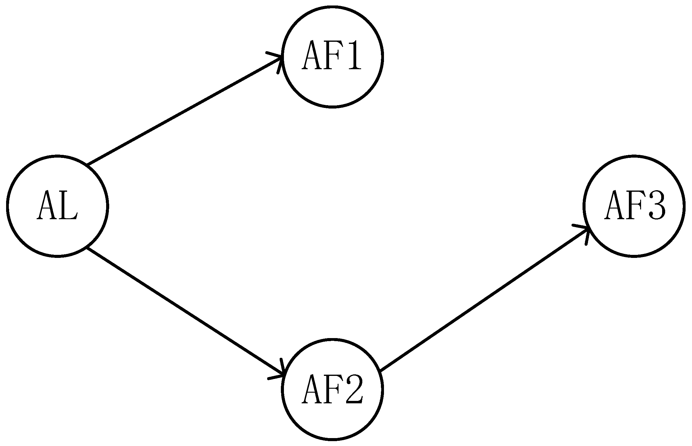
2.2. Description of the Communication Topologies
3. Main Results
3.1. Event-Triggering Mode
3.2. Trajectory-Tracking Controller Design with Predefined Performance Constraints
3.3. Yaw Angle Controller Design
3.4. Velocity Controller Design
3.5. Zeno Behavior Analysis
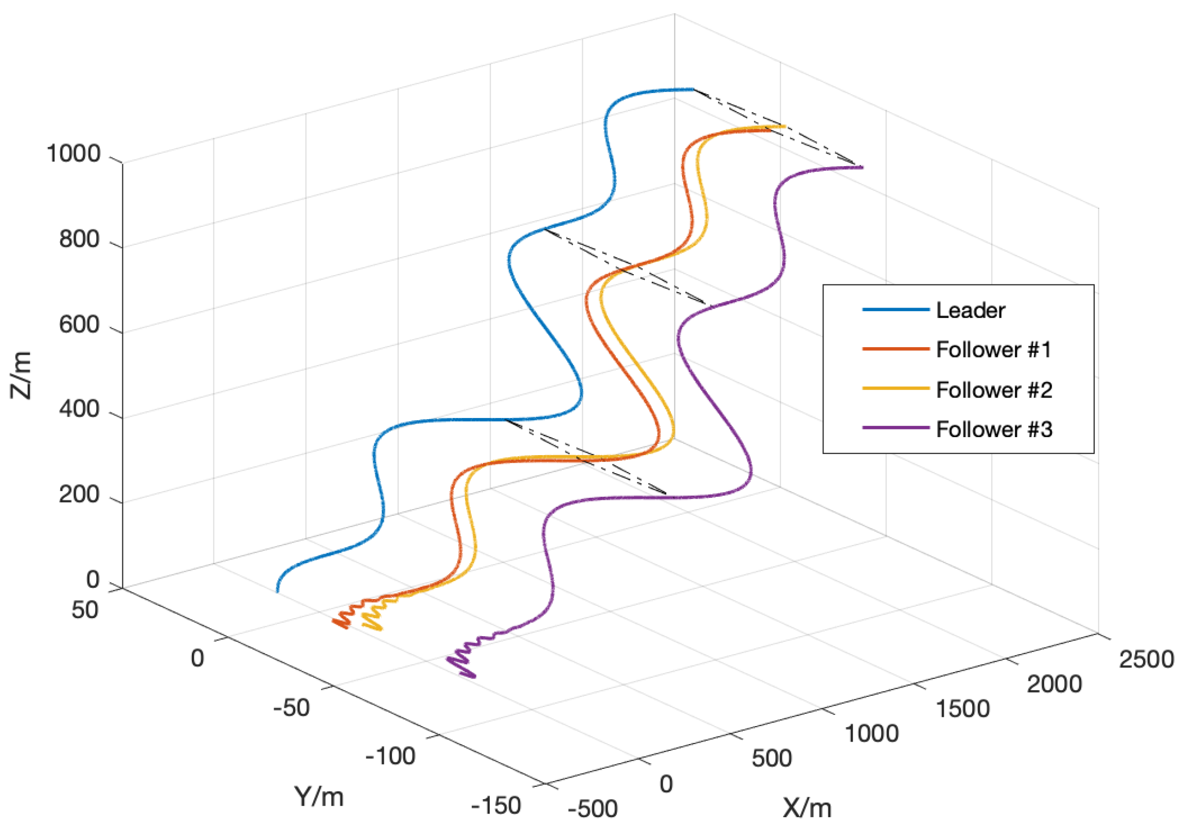
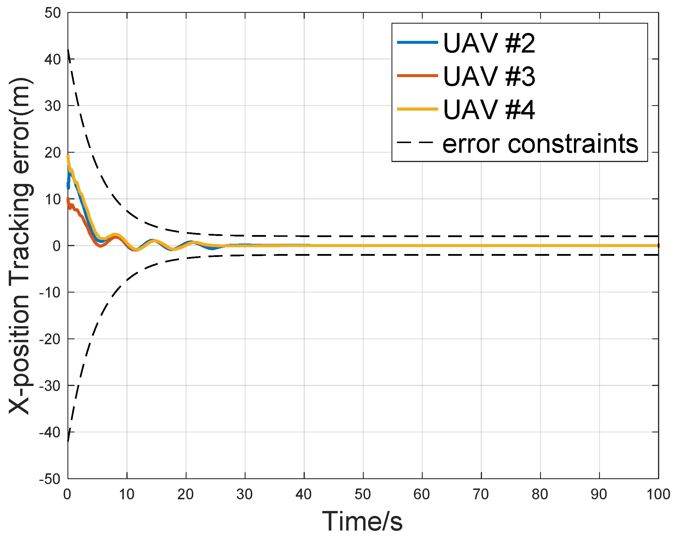
4. Simulation Results
5. Conclusions
Author Contributions
Funding
Institutional Review Board Statement
Informed Consent Statement
Data Availability Statement
Conflicts of Interest
Appendix A
References
- Muslimov, T.Z.; Munasypov, R.A. Consensus-based cooperative control of parallel fixed-wing UAV formations via adaptive backstepping. Aerosp. Sci. Technol. 2021, 109, 106416. [Google Scholar] [CrossRef]
- Muslimov, T.Z.; Munasypov, R.A. Adaptive decentralized flocking control of multi-UAV circular formations based on vector fields and backstepping. ISA Trans. 2020, 107, 143–159. [Google Scholar] [CrossRef]
- Wei, L.; Chen, M.; Li, T. Disturbance-observer-based formation-containment control for UAVs via distributed adaptive event-triggered mechanisms. J. Frankl. Inst. 2021, 358, 5305–5333. [Google Scholar] [CrossRef]
- Zhang, Y.; Li, S.; Wang, S.; Wang, X.; Duan, H. Distributed bearing-based formation maneuver control of fixed-wing UAVs by finite-time orientation estimation. Aerosp. Sci. Technol. 2023, 136, 108241. [Google Scholar] [CrossRef]
- Chen, J.; Yang, W.; Shi, Z.; Zhong, Y. Robust horizontal-plane formation control for small fixed-wing UAVs. Aerosp. Sci. Technol. 2022, 131, 107958. [Google Scholar] [CrossRef]
- Yan, D.; Zhang, W.; Chen, H.; Shi, J. Robust control strategy for multi-UAVs system using MPC combined with Kalman-consensus filter and disturbance observer. ISA Trans. 2023, 135, 35–51. [Google Scholar] [CrossRef] [PubMed]
- Zhen, Z.; Zhu, P.; Xue, Y.; Ji, Y. Distributed intelligent self-organized mission planning of multi-UAV for dynamic targets cooperative search-attack. Chin. J. Aeronaut. 2019, 32, 2706–2716. [Google Scholar] [CrossRef]
- Hu, J.; Niu, H.; Carrasco, J.; Lennox, B.; Arvin, F. Fault-tolerant cooperative navigation of networked UAV swarms for forest fire monitoring. Aerosp. Sci. Technol. 2022, 123, 107494. [Google Scholar] [CrossRef]
- Zhao, Z.; Niu, Y.; Shen, L. Adaptive level of autonomy for human-UAVs collaborative surveillance using situated fuzzy cognitive maps. Chin. J. Aeronaut. 2020, 33, 2835–2850. [Google Scholar] [CrossRef]
- Cai, Z.; Wang, L.; Zhao, J.; Wu, K.; Wang, Y. Virtual target guidance-based distributed model predictive control for formation control of multiple UAVs. Chin. J. Aeronaut. 2020, 33, 1037–1056. [Google Scholar] [CrossRef]
- Wang, Y.; Zhang, T.; Cai, Z.; Zhao, J.; Wu, K. Multi-UAV coordination control by chaotic grey wolf optimization based distributed MPC with event-triggered strategy. Chin. J. Aeronaut. 2020, 33, 2877–2897. [Google Scholar] [CrossRef]
- Guo, S.; Li, Z.; Niu, Y.; Wu, L. Consensus disturbance rejection control of directed multi-agent networks with extended state observer. Chin. J. Aeronaut. 2020, 33, 1486–1493. [Google Scholar] [CrossRef]
- Han, L.; Dong, X.; Li, Q.; Ren, Z. Formation tracking control for time-delayed multi-agent systems with second-order dynamics. Chin. J. Aeronaut. 2017, 30, 348–357. [Google Scholar] [CrossRef]
- Liang, Y.; Dong, Q.; Zhao, Y. Adaptive leader–follower formation control for swarms of unmanned aerial vehicles with motion constraints and unknown disturbances. Chin. J. Aeronaut. 2020, 33, 2972–2988. [Google Scholar] [CrossRef]
- Yang, W.; Chen, J.; Zhang, Z.; Shi, Z.; Zhong, Y. Robust cascaded horizontal-plane trajectory tracking for fixed-wing unmanned aerial vehicles. J. Frankl. Inst. 2022, 359, 1083–1112. [Google Scholar] [CrossRef]
- Zhi, Y.; Liu, L.; Guan, B.; Wang, B.; Cheng, Z.; Fan, H. Distributed robust adaptive formation control of fixed-wing UAVs with unknown uncertainties and disturbances. Aerosp. Sci. Technol. 2022, 126, 107600. [Google Scholar] [CrossRef]
- Lungu, M. Auto-landing of UAVs with variable centre of mass using the backstepping and dynamic inversion control. Aerosp. Sci. Technol. 2020, 103, 105912. [Google Scholar] [CrossRef]
- Sun, R.; Zhou, Z.; Zhu, X. Stability control of a fixed full-wing layout UAV under manipulation constraints. Aerosp. Sci. Technol. 2022, 120, 107263. [Google Scholar] [CrossRef]
- Zhang, B.; Sun, X.; Lv, M. Distributed adaptive specified-time synchronization tracking of multiple 6-DOF fixed-wing UAVs with guaranteed performances. ISA Trans. 2022, 129, 260–272. [Google Scholar] [CrossRef]
- Chen, K.; Zhu, S.; Wei, C.; Xu, T.; Zhang, X. Output constrained adaptive neural control for generic hypersonic vehicles suffering from non-affine aerodynamic characteristics and stochastic disturbances. Aerosp. Sci. Technol. 2021, 111, 106469. [Google Scholar] [CrossRef]
- Hu, B.; Guan, Z.H.; Lewis, F.L.; Chen, C.P. Adaptive Tracking Control of Cooperative Robot Manipulators With Markovian Switched Couplings. IEEE Trans. Ind. Electron. 2021, 68, 2427–2436. [Google Scholar] [CrossRef]
- Yu, Z.; Zhang, Y.; Jiang, B.; Yu, X.; Fu, J.; Jin, Y.; Chai, T. Distributed adaptive fault-tolerant close formation flight control of multiple trailing fixed-wing UAVs. ISA Trans. 2020, 106, 181–199. [Google Scholar] [CrossRef] [PubMed]
- Chen, S.; Chen, Z. On Active Disturbance Rejection Control for a Class of Uncertain Systems With Measurement Uncertainty. IEEE Trans. Ind. Electron. 2021, 68, 1475–1485. [Google Scholar] [CrossRef]
- Wang, X.; Guo, J.; Tang, S.; Qi, S. Fixed-time disturbance observer based fixed-time back-stepping control for an air-breathing hypersonic vehicle. ISA Trans. 2019, 88, 233–245. [Google Scholar] [CrossRef] [PubMed]
- Dong, C.; Liu, Y.; Wang, Q. Barrier Lyapunov function based adaptive finite-time control for hypersonic flight vehicles with state constraints. ISA Trans. 2020, 96, 163–176. [Google Scholar] [CrossRef] [PubMed]
- Su, Z.; Li, C.; Wang, H. Barrier Lyapunov function-based robust flight control for the ultra-low altitude airdrop under airflow disturbances. Aerosp. Sci. Technol. 2019, 84, 375–386. [Google Scholar] [CrossRef]
- Liu, K.; Yang, P.; Wang, R.; Jiao, L.; Li, T.; Zhang, J. Observer-based adaptive fuzzy finite-time attitude control for quadrotor UAVs. IEEE Trans. Aerosp. Electron. Syst. 2023, 59, 8637–8654. [Google Scholar] [CrossRef]
- Liu, K.; Yang, P.; Jiao, L.; Wang, R.; Yuan, Z.; Dong, S. Antisaturation fixed-time attitude tracking control based low-computation learning for uncertain quadrotor UAVs with external disturbances. Aerosp. Sci. Technol. 2023, 142, 108668. [Google Scholar] [CrossRef]
- Huang, Y.; Wang, J.; Shi, D.; Shi, L. Toward Event-Triggered Extended State Observer. IEEE Trans. Autom. Control 2018, 63, 1842–1849. [Google Scholar] [CrossRef]
- Zhen, Z.; Tao, G.; Xu, Y.; Song, G. Multivariable adaptive control based consensus flight control system for UAVs formation. Aerosp. Sci. Technol. 2019, 93, 105336. [Google Scholar] [CrossRef]
- Yu, Z.; Zhang, Y.; Liu, Z.; Qu, Y.; Su, C.; Jiang, B. Decentralized finite-time adaptive fault-tolerant synchronization tracking control for multiple UAVs with prescribed performance. J. Frankl. Inst. 2020, 357, 11830–11862. [Google Scholar] [CrossRef]
- Xu, B.; Shi, Z.; Sun, F.; He, W. Barrier Lyapunov Function Based Learning Control of Hypersonic Flight Vehicle with AOA Constraint and Actuator Faults. IEEE Trans. Cybern. 2019, 49, 1047–1057. [Google Scholar] [CrossRef]
- Yuan, Y.; Wang, Z.; Guo, L.; Liu, H. Barrier Lyapunov Functions-Based Adaptive Fault Tolerant Control for Flexible Hypersonic Flight Vehicles With Full State Constraints. IEEE Trans. Syst. Man Cybern. Syst. 2020, 50, 3391–3400. [Google Scholar] [CrossRef]
- Zhou, W.; Li, J.; Liu, Z.; Shen, L. Improving multi-target cooperative tracking guidance for UAV swarms using multi-agent reinforcement learning. Chin. J. Aeronaut. 2022, 35, 100–112. [Google Scholar] [CrossRef]
- Abbaspour, A.; Yen, K.K.; Forouzannezhad, P.; Sargolzaei, A. A Neural Adaptive Approach for Active Fault-Tolerant Control Design in UAV. IEEE Trans. Syst. Man Cybern. Syst. 2020, 50, 3401–3411. [Google Scholar] [CrossRef]
- Sun, J.; Yang, J.; Li, S.; Zheng, W.X. Sampled-Data-Based Event-Triggered Active Disturbance Rejection Control for Disturbed Systems in Networked Environment. IEEE Trans. Cybern. 2019, 49, 556–566. [Google Scholar] [CrossRef]
- Hua, Y.; Dong, X.; Li, Q.; Ren, Z. Distributed fault-tolerant time-varying formation control for high-order linear multi-agent systems with actuator failures. ISA Trans. 2017, 71, 40–50. [Google Scholar] [CrossRef]
- Yu, Z.; Zhang, Y.; Jiang, B.; Su, C.; Fu, J.; Jin, Y.; Chai, T. Decentralized fractional-order backstepping fault-tolerant control of multi-UAVs against actuator faults and wind effects. Aerosp. Sci. Technol. 2020, 104, 105939. [Google Scholar] [CrossRef]
- Yu, Z.; Qu, Y.; Zhang, Y. Distributed Fault-Tolerant Cooperative Control for Multi-UAVs Under Actuator Fault and Input Saturation. IEEE Trans. Control Syst. Technol. 2019, 27, 2417–2429. [Google Scholar] [CrossRef]
- Yu, Z.; Zhang, Y.; Jiang, B.; Yu, X. Fault-Tolerant Time-Varying Elliptical Formation Control of Multiple Fixed-Wing UAVs for Cooperative Forest Fire Monitoring. J. Intell. Robot. Syst. 2021, 101, 1–15. [Google Scholar] [CrossRef]
- Yu, Z.; Qu, Y.; Zhang, Y. Safe control of trailing UAV in close formation flight against actuator fault and wake vortex effect. Aerosp. Sci. Technol. 2018, 77, 189–205. [Google Scholar] [CrossRef]
- Administration, F.A. Pilot’s Handbook of Aeronautical Knowledge; Skyhorse Publishing Inc.: New York, NY, USA, 2009. [Google Scholar]
- Bayezit, I.; Fidan, B. Distributed cohesive motion control of flight vehicle formations. IEEE Trans. Ind. Electron. 2012, 60, 5763–5772. [Google Scholar] [CrossRef]
- Karimoddini, A.; Lin, H.; Chen, B.M.; Lee, T.H. Hybrid three-dimensional formation control for unmanned helicopters. Automatica 2013, 49, 424–433. [Google Scholar] [CrossRef]
- Wang, Y.; Wang, D.; Zhu, S. Cooperative moving path following for multiple fixed-wing unmanned aerial vehicles with speed constraints. Automatica 2019, 100, 82–89. [Google Scholar] [CrossRef]
- Broomhead, D.; Lowe, D. Radial Basis Functions, Multi-Variable Functional Interpolation and Adaptive Networks; Royal Signals and Radar Establishment Malvern: Worcestershire, UK, 1988. [Google Scholar]
- Cruz-Zavala, E.; Moreno, J.A.; Fridman, L.M. Uniform robust exact differentiator. IEEE Trans. Autom. Control 2011, 56, 2727–2733. [Google Scholar] [CrossRef]
- Su, B.; Wang, H.; Wang, Y.; Gao, J. Event-triggered formation control for AUVs with fixed-time sliding mode disturbance observer. Control Decis. 2022, 37, 1116–1126. [Google Scholar] [CrossRef]
- Liu, K.; Wang, R.; Zheng, S.; Dong, S.; Sun, G. Fixed-time disturbance observer-based robust fault-tolerant tracking control for uncertain quadrotor UAV subject to input delay. Nonlinear Dyn. 2022, 107, 2363–2390. [Google Scholar] [CrossRef]
- Liu, K.; Wang, R. Antisaturation adaptive fixed-time sliding mode controller design to achieve faster convergence rate and its application. IEEE Trans. Circuits Syst. II Express Briefs 2022, 69, 3555–3559. [Google Scholar] [CrossRef]
- Hosseinzadeh, M.; Yazdanpanah, M.J. Performance enhanced model reference adaptive control through switching non-quadratic Lyapunov functions. Syst. Control Lett. 2015, 76, 47–55. [Google Scholar] [CrossRef]
- Tao, G. Model reference adaptive control with L1+α tracking. Int. J. Control 1996, 64, 859–870. [Google Scholar] [CrossRef]


| UAV (1,2,3) | Initial State | Desired Position with the Leader |
|---|---|---|
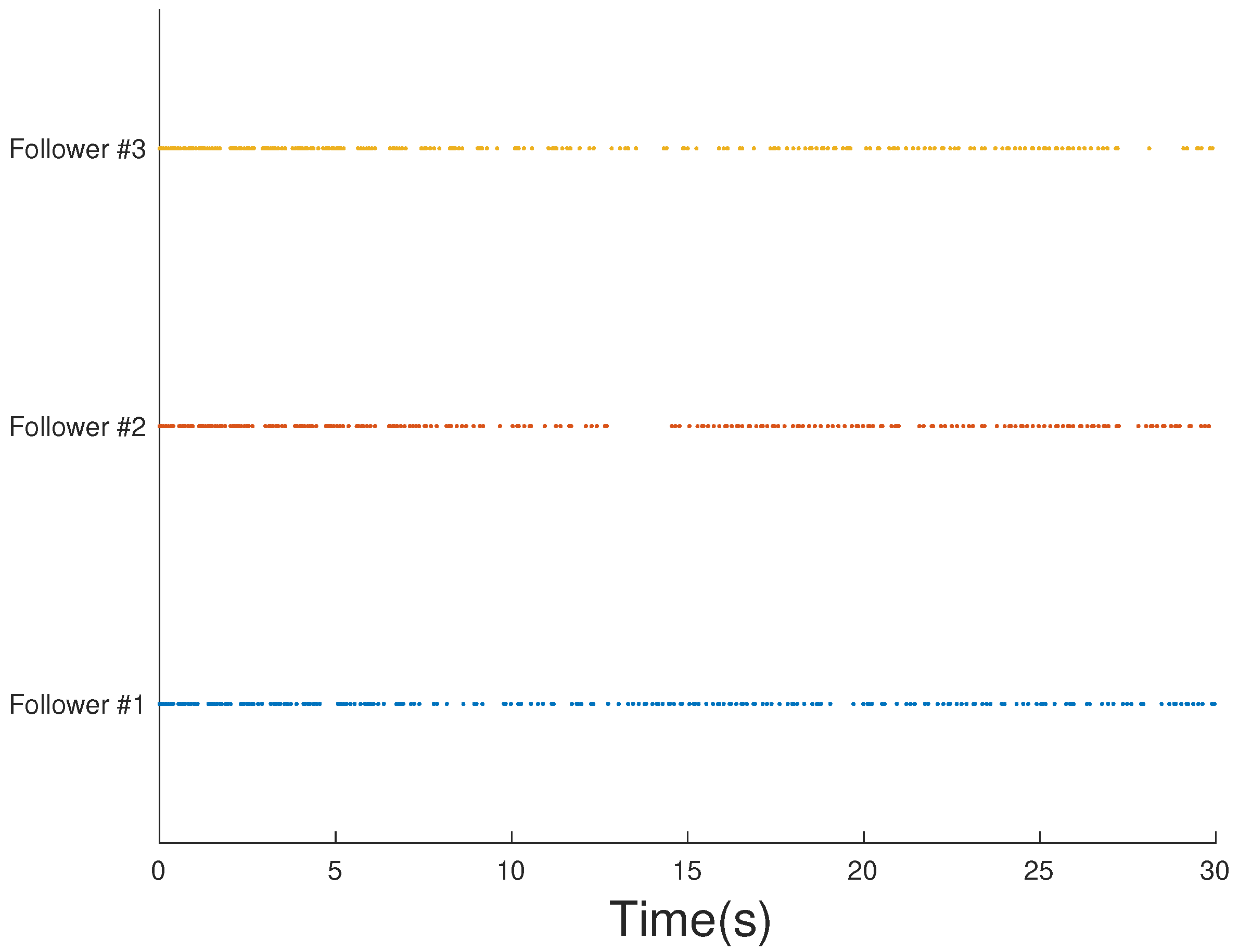
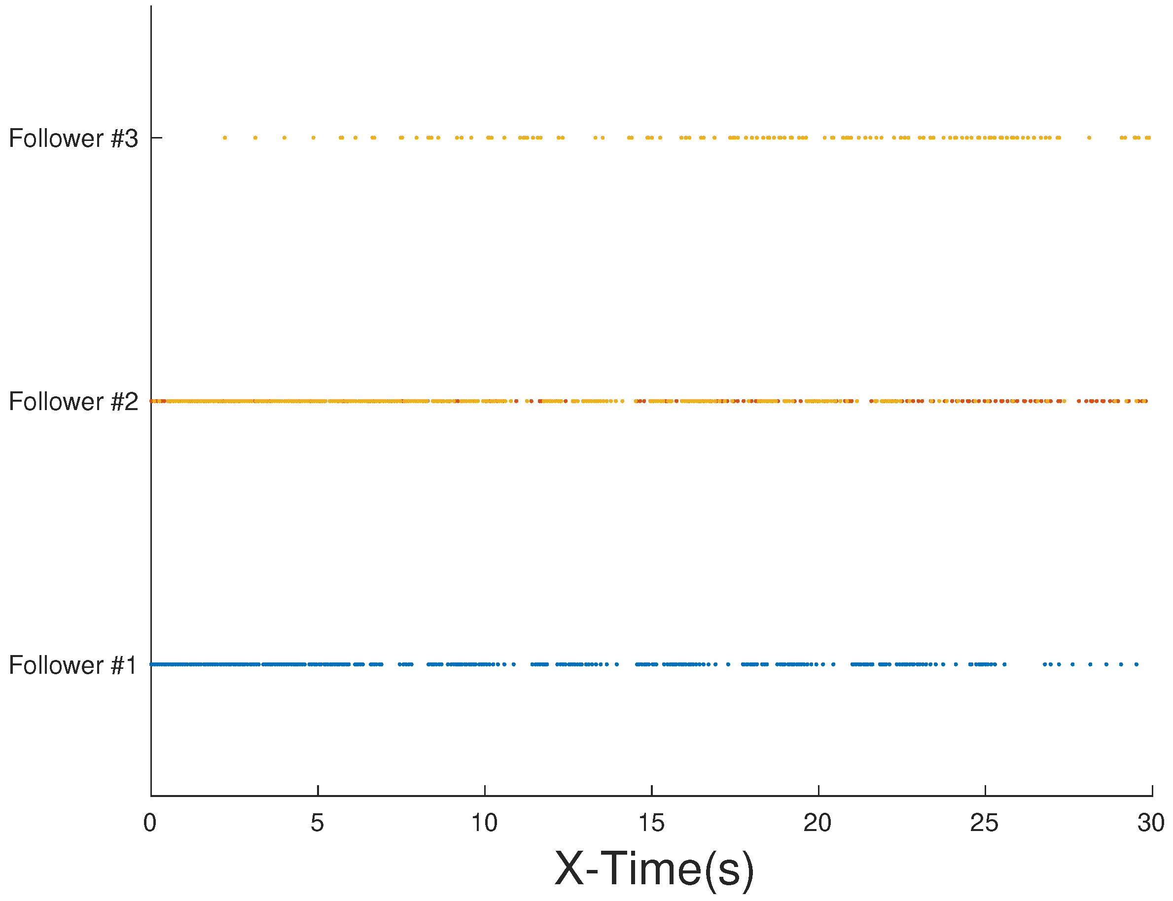
| UAV No. | Heading Angle Control Time Interval | Velocity Control Time Interval | ||||
|---|---|---|---|---|---|---|
| Minimum Time (s) | Maximum Time (s) | Average Time (s) | Minimum Time (s) | Maximum Time (s) | Average Time (s) | |
| UAV 1 | 0.010 | 0.970 | 0.124 | 0.010 | 2.390 | 0.118 |
| UAV 2 | 0.010 | 1.850 | 0.120 | 0.010 | 2.040 | 0113 |
| UAV 3 | 0.010 | 1.130 | 0.121 | 0.010 | 3.780 | 0.097 |
Disclaimer/Publisher’s Note: The statements, opinions and data contained in all publications are solely those of the individual author(s) and contributor(s) and not of MDPI and/or the editor(s). MDPI and/or the editor(s) disclaim responsibility for any injury to people or property resulting from any ideas, methods, instructions or products referred to in the content. |
© 2024 by the authors. Licensee MDPI, Basel, Switzerland. This article is an open access article distributed under the terms and conditions of the Creative Commons Attribution (CC BY) license (https://creativecommons.org/licenses/by/4.0/).
Share and Cite
Ma, Z.; Gong, H.; Wang, X. Fault-Tolerant Event-Triggrred Control for Multiple UAVs with Predefined Tracking Performance. Drones 2024, 8, 25. https://doi.org/10.3390/drones8010025
Ma Z, Gong H, Wang X. Fault-Tolerant Event-Triggrred Control for Multiple UAVs with Predefined Tracking Performance. Drones. 2024; 8(1):25. https://doi.org/10.3390/drones8010025
Chicago/Turabian StyleMa, Ziyuan, Huajun Gong, and Xinhua Wang. 2024. "Fault-Tolerant Event-Triggrred Control for Multiple UAVs with Predefined Tracking Performance" Drones 8, no. 1: 25. https://doi.org/10.3390/drones8010025
APA StyleMa, Z., Gong, H., & Wang, X. (2024). Fault-Tolerant Event-Triggrred Control for Multiple UAVs with Predefined Tracking Performance. Drones, 8(1), 25. https://doi.org/10.3390/drones8010025