Abstract
UAVs flying in complex low-altitude environments often require real-time sensing to avoid
environmental obstacles. In previous approaches, UAVs have usually carried out motion planning
based on primitive navigation maps such as point clouds and raster maps to achieve autonomous
obstacle avoidance. However, due to the huge amount of data in these raw navigation maps and the
highly discrete map information, the efficiency of solving the UAV’s real-time trajectory optimization
is low, making it difficult to meet the demand for efficient online motion planning. A flight corridor is
a series of unobstructed continuous areas and has convex properties. The flight corridor can be used
as a simple parametric representation to characterize the safe flight space in the environment, and
used as the cost of the collision term in the trajectory back-end optimization for trajectory solving,
which can improve the efficiency of real-time trajectory solving and ensure flight safety. Therefore,
this paper focuses on the construction of safe flight corridors for UAVs and autonomous obstacle
avoidance algorithms for UAVs based on safe flight corridors, based on a rotary-wing UAV platform,
and proposes a polyhedral flight corridor construction algorithm and realizes autonomous obstacle
avoidance for UAVs based on the constructed flight corridors.
1. Introduction
Rotorcraft drones have the characteristics of strong portability, high maneuverability, vertical takeoff and landing capability, simple aerodynamic principles, and low cost [1], and have become the focus of research by major research institutes and commercial companies [2]. In the military field, rotorcraft drones can be used for low-altitude reconnaissance and swarm warfare. In the civilian field, rotorcraft drones can be used for disaster relief, surveying and monitoring, aerial photography, and delivery services. In these low-altitude complex environments, autonomous drones need to obtain environmental information through onboard sensors and be able to plan a dynamic obstacle avoidance route. How to dynamically perceive the surrounding environment and plan flight routes has become an important research direction in the field of drone obstacle avoidance. However, due to the limitations of the drone’s own size, the implementation of its autonomous obstacle avoidance technology is constrained by SWaP (Size, Weight, and Power), often requiring it to utilize limited onboard computing resources to complete real-time and efficient flight trajectory calculations. Therefore, how to construct an environment and efficiently solve the real-time obstacle avoidance trajectory of unmanned aerial vehicles, that is, the motion planning problem of unmanned aerial vehicles during obstacle avoidance, is the research focus of autonomous obstacle avoidance technology for unmanned aerial vehicles.
In practical obstacle avoidance planning for unmanned aerial vehicles, there are two challenges [3]. Firstly, real-time trajectories need to be continuously based on environmental information for trajectory replanning. Therefore, it is necessary to quickly solve real-time trajectories under the condition of lightweight airborne computing resources. Secondly, online trajectory optimization solutions are often complex. The expression form of constraint conditions and trajectories greatly affects the speed of trajectory solving. In order to address these two challenges, many studies have been conducted in fields such as mapping and planning. Previous methods of obstacle avoidance have usually been based on point clouds and raster maps for motion planning, but the high level of discrete map information and the large amount of data available have led to inefficient real-time trajectory solving. The dense map used for autonomous obstacle avoidance can be roughly divided into a point cloud map, occupancy grid map, and its extension types, including Octomap and Signed Distance Field (SDF), etc. A safe flight corridor is a series of obstacle-free areas based on point clouds, raster maps, and other maps that mark obstacles, often with convex shapes and interconnections, thus forming a corridor that can be flown freely. Previously, in SDF maps or other maps that measure gradients based on distance, environmental gradient information was almost always non-convex, and solving a non-convex problem online was often very complex and may not even have been able to find the optimal solution. The flight corridors can be used to characterize safe flight spaces through simple parametric representations, improving the efficiency of real-time trajectory solving and ensuring flight safety. The flight corridor can transform non-convex spatial information into convex spatial information through the flight corridor construction algorithm, that is, transform the optimization problem into a convex optimization problem, which can improve the efficiency and quality of the optimization solution. Therefore, the study of the construction method of flight corridors and the motion planning method based on flight corridors are of great significance to the UAV autonomous obstacle avoidance technology. This paper addresses the need for the rapid solution of UAV obstacle avoidance trajectories by constructing a safe flight corridor for UAVs in the context of the study of autonomous obstacle avoidance algorithms for rotary-wing UAVs in complex low-altitude environments.
The contributions of this paper are summarized as follows:
- 1.
- In response to the problem of overly complex characterization of the UAV flight environment with the original navigation map, a flight corridor construction method based on geometric space expansion and cutting is proposed.
- 2.
- A UAV autonomous obstacle avoidance algorithm based on the flight corridor for motion planning is proposed to address the problem of the low efficiency of online real-time trajectory solving for UAVs.
The remainder of this manuscript is structured as follows. Section 2 introduces some related works of autonomous obstacle avoidance methods for drones. Section 3 constructs a polyhedral flight corridor and implements autonomous obstacle avoidance based on the corridor. Experimental results are presented in Section 4 to validate the effectiveness of our proposed method. Section 5 concludes this paper and envisages some future work.
2. Related Works
2.1. Autonomous Obstacle Avoidance Algorithms for UAV
In 2011, Daniel et al. proposed the Minimum Snap method, which uses the idea of optimization to solve a trajectory generation problem [4], which generates a real-time optimal trajectory from a series of 3D coordinates and yaw angles, using a polynomial representation of the trajectory and ensuring that the trajectory satisfies dynamical constraints as well as safety constraints.
When the number of segments of a polynomial curve is too large, the order of its curve increases and the efficiency of the solution decreases. Vlady et al. used a trajectory representation of the B spline to parametrically represent the trajectory [5], which has convex wrapper properties that allow the trajectory to be completely confined to a convex wrapper consisting of control points, and therefore only constraining the control points can control the shape of the trajectory. The Fast-Planner [6] and EGO-Planner [7] algorithms, which have made a big splash in the field of UAV motion planning in recent years, both use the B-sample trajectory representation.
The EGO-v2 [8], which appeared on the cover of the science subjournal Robotics in 2022, uses the trajectory class MINCO (Minimum Control) [9] proposed by Wang et al. This trajectory class is still essentially a polynomial trajectory but is built under the condition of higher-order derivative continuity of the trajectory, which can guarantee the spatio-temporal optimality of the trajectory while efficiently handling various constraints. That is, the MINCO trajectory class is a trajectory expression parametrized in terms of both spatial location q and time t. MINCO can also calculate the analytical solution of the trajectory generation directly by matrix operations, which can avoid the inefficiency of solving numerical solutions and solve the optimality of time allocation.
In summary, in the current research on motion planning algorithms, optimization-based approaches ensure that trajectories are both safe and feasible and easy to deploy in realistic scenarios. However, the smoothness, dynamical feasibility, and safety of the trajectory need to be considered in the process of optimizing the trajectory.
In [5,6,7], the distance gradient information between the current position of the UAV and the obstacles is used to achieve the collision term constraints on the UAV (the further the distance, the smaller the possibility of collision), and motion planning was performed directly in the original navigation map. However, the 3D map data are highly discrete and the data volume is huge; the distance gradient data are highly non-convex, which is not conducive to efficient solving of real-time trajectories. Based on the need for optimal trajectory solving, the concept of flight corridors is proposed in Refs. [10,11,12], enabling UAV motion planning using flight corridors. By constructing a real-time flight corridor, the UAV achieves the transformation of the non-convex map environment information to the convex corridor environment information, and constrains the UAV flight trajectory inside the flight corridor, thus achieving safe collision avoidance. Although constructing the corridor requires a small number of additional operations, it is more efficient to solve the optimal trajectory in convex space. Therefore, the obstacle avoidance planning method based on flight corridors is of great research significance, and how to construct the flight corridor is the research focus of this method.
2.2. Flight Corridor Construction Algorithm
Ref. [13] constructs spherical flight corridors, which are constructed in a map data structure based on a KD tree representation. As the safe radius of any point in the map can be found by the fast nearest neighbor search method in the KD tree, the distance from the coordinate point to the nearest obstacle can be easily obtained, and the distance is used as the radius of the spherical corridor. A random sampling-based method is used to connect the path from the starting point to the target point, and the points on that path are used to construct a continuous spherical corridor. Ref. [14] further improves on NanoMap [15] by iteratively checking whether the query point is in the in-frame view in order to obtain the distance from the nearest point to the drone, and estimating the uncertainty of the query. Then, using a KD tree, the nearest neighbor point is found and a spherical corridor is generated along the path. The advantage of a spherical corridor is that it is simple to construct, requiring only one parameter, the safety radius, to be found to construct a sphere. However, spherical corridors are less space efficient and have less free space for path optimization. Ref. [16] builds cubic flight corridors based on octree maps, which have axes parallel to the coordinate axes, and the corridors also expand axially. However, the construction method in [16] is more dependent on the octree map environment, and the space utilization of this type of corridor is low due to the geometric properties of the octree structure itself in space. Ref. [17] proposes a cube corridor construction method that finds the maximum radius sphere by constructing an ESDF map and then expands the inner cube of this sphere axially, which does not rely on the octree map structure and therefore can contain more free space. The advantage of a cubic corridor is that the space is easy to represent and can be simply parametrized by the intersection of the six surfaces of the corridor space with the corresponding axes, i.e., by restricting the coordinate points to the upper and lower bounds represented by the and z axes. However, in highly non-convex spaces, polyhedra can often contain more free space than axially extended cubes [10].
3. Proposed Method
3.1. Overview
The autonomous drone needs to obtain the current position information and the movement information of the airframe in real time during the flight, relying on the onboard sensors to sense the surrounding environment. A trajectory that does not collide with environmental obstacles in a safe flight area is planned in real time, and then the controller controls the drone to follow the planned trajectory. Based on the above description, we designed an experimental system framework that includes the autonomous positioning module, mapping module, motion planning module, and flight control module, as shown in Figure 1.
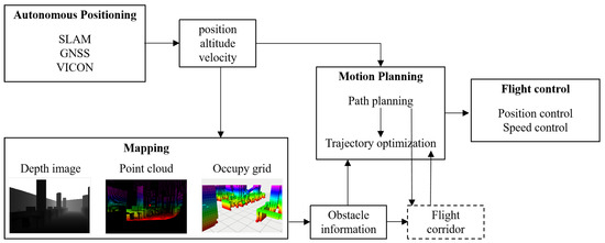
Figure 1.
The framework of UAV autonomous obstacle avoidance system includes autonomous positioning, perceptual mapping, motion planning, and flight control, while the flight corridor takes map and path as input, and acts in trajectory optimization.
- (1)
- Autonomous positioning module. In the autonomous positioning module, the UAV uses sensors and external environmental information to determine its current position and direction of movement. When encountering obstacles, drones need to combine the location information of the obstacles and their own location information to plan a new local path to ensure flight safety. Common methods of obtaining a UAV’s position include visual SLAM, radar SLAM, and GNSS systems, while motion capture systems can also be used to assist in obtaining precise indoor positioning of the UAV.
- (2)
- Mapping module. In the sensory map building module, the UAV acquires environmental information, including terrain, obstacle locations, obstacle contours, etc., through the mounted sensory sensors and passes this information to the onboard computer to build an environmental map for path planning.
- (3)
- Motion planning module. The planning module is usually divided into two parts: front-end path planning and back-end trajectory optimization. Path planning finds a path that connects the starting point to the endpoint, while trajectory optimization optimizes this path to meet the actual flight requirements. The planning module is the core module of the UAV’s autonomous obstacle avoidance algorithm. Its role is to receive the UAV’s own positioning information and environmental map information and to find an optimal trajectory that can guide the UAV from the current point to the target point through the motion planning algorithm. The quality of the trajectory solved by the planning module directly affects whether the UAV can avoid the obstacle. The flight corridor, on the other hand, is used in the planning module as a collision term cost for trajectory optimization, ensuring the safety of the trajectory.
- (4)
- Flight control module. The control module is responsible for tracking the trajectory output from the UAV planning module, which is usually represented by a number of dense but discrete coordinate points. Based on the position and attitude information obtained by the positioning module, the flight control controls the aircraft to follow a predetermined path point, for example, by changing the flight altitude, direction, or speed to avoid obstacles and ensure the safe flight of the UAV. During the flight, the control module needs to solve the flight altitude and flight speed needed to track the path in real time and also needs to monitor its own flight status in real time.
The design of this framework structure is used to guide us in designing actual physics experimental systems for outdoor flight experimental verification. In the above modules, we focus on how to quickly construct flight corridors using SDF maps and guide the optimization of local obstacle avoidance flight paths based on the flight corridor.
3.2. Path Planning
The core technology of autonomous obstacle avoidance for unmanned aerial vehicles is the motion planning algorithm, which usually includes front-end path planning and back-end trajectory optimization. Drones rely on spatial obstacle information obtained from onboard sensors to construct an environmental map for the autonomous navigation of drones and use path replanning algorithms to find flight paths in space. In research on front-end path planning, commonly used methods include graph-based searches such as the Dijkstra [18] and A* algorithms [19], as well as search-based methods such as RRT* [20] and PRM [21]. However, due to the fact that the RRT * and PRM path points are not connected according to the shortest distance, the algorithm itself cannot find an optimal path. Although the A* and Dijkstra algorithms can find the theoretical optimal path, the continuous search of the raster space will occupy a large amount of memory and consume a large amount of computation time, which is difficult to adapt to the demand of fast trajectory replanning. In this paper, we improve the A* algorithm using the jump point search (JPS) method [11] to solve the above two problems.
The A* algorithm is a breadth-first search algorithm that starts from the starting point, iterates through the neighborhoods, and selects the optimal neighborhoods to spread outwards through the cost function until the endpoint is reached. In this case, the openlist is used to store all the non-obstructive neighboring nodes around the current point, and the closelist is used to store the least expensive point in the current openlist to reach the target point. Since the A* algorithm’s rule for exploring surrounding nodes is to traverse them one by one, i.e., the A* algorithm adds all non-obstacle points around the current point to the openlist for a single cost function calculation, this greatly increases the algorithm’s computation time. If the number of points added to the openlist could be reduced, such frequent and useless computations could be avoided. Compared to the A* algorithm, there are two new concepts in the JPS algorithm: forced neighbors and jump points.
- (1)
- The forced neighbors
If a neighboring node of a node C contains an obstacle, define N (Neighbor) to be a neighboring node of C (Current) and P (Parent) to be the parent of C. N is said to be a forced neighbor of C if the distance cost of P to reach N via C is less than the distance cost of either path to N without going through C. Figure 2 shows the forced neighbors for linear as well as diagonal motion, respectively.
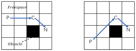
Figure 2.
Two ways of judging forced neighbor nodes: the left diagram shows a forced neighbor with straight-line movement and the right diagram shows a forced neighbor with diagonal movement.
- (2)
- The jumping points
There are three ways to determine whether point C is a jump point.
I: point C is the start or end point.
II: point C has at least one forced neighbor node.
III: if P to C is a diagonal movement and the point C can reach the jump point after a horizontal or vertical movement.
Figure 3 shows the jump points in the above three cases. In Figure 3, it can be seen that a jump point is actually a point that causes the path to move in a different direction during the graph search. Unlike the A* algorithm, which only adds jump points to the openlist, A* treats all non-obstacle points around the current node as neighbors and adds them to the openlist. As a result, the JPS algorithm is usually more computationally efficient due to the fact that it performs fewer operations on the openlist.
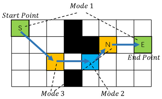
Figure 3.
There are three ways of determining jump points, green for type 1, blue for type 2, and yellow for type 3.
At the same time, as the sensing sensors are usually forward mounted during the flight of the UAV, there is little sensing capability in the z-axis direction. When performing path planning, it is desired to reduce the motion process of the UAV in the z-axis direction. Therefore, the cost function of the JPS is designed in this paper as:
where denotes the cost of moving from the starting point to the point to be examined and denotes the predicted cost from the point to be examined to the target point. The for a body raster that is at the same height as the current raster. For rasters at different heights from the current raster, , as shown in Figure 4.
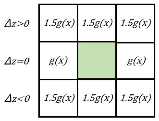
Figure 4.
Adding additional constraints to the movement of the z-axis reduces the height variation during path planning.
3.3. Flight Corridors’ Design
A safe flight corridor (SFC) is a series of barrier-free zones built from maps with point clouds or raster maps. These zones often have a convex shape and are interconnected, creating a corridor through which the air vehicle can fly freely. A safe flight corridor is a set of convex geometric objects that satisfy safety, convexity, and continuity. In related research, commonly used convex aggregates include spheres, cubes, and convex polyhedrons. According to the above definition, safe flight corridors should have the following characteristics.
- (1)
- Safety: The path and the drone are contained within the corridor and the obstacles are outside the corridor.where denotes the path (a series of ), represents a convex set containing all vertices of a drone (Quadrotor), represents a convex set composed of vertices of a single obstacle, (Obstacle) is a set of , and is the set of all segments of the flight corridor combined: .
- (2)
- Convexity: Every segment of corridor is a convex geometry. Define any two points and within any segment of corridor space, then any point on the line segment formed by these two points is contained within the corridor.
- (3)
- Continuity: Each segment of the flight corridor is continuous from front to back, and the two endpoints of the path are contained within the flight corridor of the corresponding path segment.
Environmental perception map information and the planned path of the drone serve as inputs, and by performing operations such as geometric expansion, compression, and segmentation on an initialized area in geometric space, the construction of flight corridors based on geometric methods can be achieved. This paper classifies different shapes of flight corridors and studies the construction methods of spherical corridors, cubic corridors, and polyhedral corridors. In order to facilitate visual presentation, this paper uses a top-down view of a two-dimensional plane to demonstrate the generation methods of the corridors.
- (1)
- The spherical flight corridor
Path planning generates a series of discrete path points in the environment, defining the midpoint of any two neighboring path points as . With as the center of the sphere, find the nearest obstacle point to the center of the sphere and write down the distance between the center of the sphere and the obstacle point as to obtain the radius of the spherical corridor [13].
During the construction of the spherical corridor, the condition of continuity of the corridor needs to be checked:
The condition is that the distance from the two endpoints of the path to the center of the sphere needs to be less than . If a segment of the spherical flight corridor does not satisfy Formula (5) after expansion, that is, this segment of the corridor does not contain all the points in the path, then it does not satisfy the continuity of the corridor. At this point, a new point needs to be inserted between by means of an interpolation of points, in this paper , and the interpolation process is shown in Figure 5.
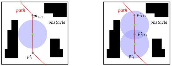
Figure 5.
When the spherical corridor does not contain the two endpoints of the path, as shown on the left, the green point in the diagram needs to be added to the queue as a new , before the corridor calculation is repeated until every point in is included in the corridor of the corresponding path segment.
In the process of implementing spherical corridor construction, an initial point location that is close to an obstacle will result in the initial radius r hitting the obstacle just as it begins to expand, and then immediately stopping the expansion, as shown in Figure 6. Although the continuity problem of spherical corridors can be solved using the interpolation of points, the final corridor may be a series of very small spheres with low space utilization.
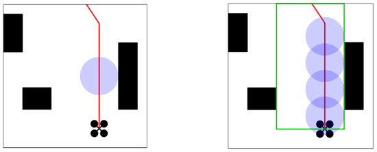
Figure 6.
The spherical corridor is underutilized and the areas in the green boxes in the diagram on the right are all safe areas.
- (2)
- The cubic corridor
To improve the space utilization of the flight corridor, inspired by the spherical flight corridor, a cube corridor can be constructed [17], as shown in Figure 7.
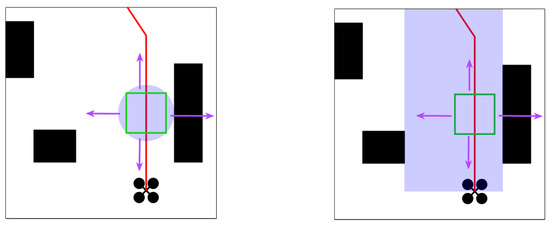
Figure 7.
Make a spherical corridor of internally connected square cubes and extend the distance from each face of the cube to the center of the sphere until you meet an obstacle to obtain a cube corridor.
The cube corridor is constructed by first finding a maximal sphere and making its inner positive cube. Then update the distance from each face of the positive cube to the center of the sphere in turn, until it stops when it encounters an obstacle. At this point, a cube corridor with greater space utilization can be obtained.
The spherical flight corridor iterates over the radius r of the expanding sphere and the cubic corridor iterates over the length l of each face to the initial point, but simple expansions for the geometric properties of spheres and cubes are limited by their geometric features to stop expanding when they hit an obstacle, preventing better space utilization.
- (3)
- The polyhedral flight corridor
This section proposes a method of constructing a flight corridor that continues to expand whether or not it hits an obstacle until it finds a convex polyhedron that satisfies the condition. The convex polyhedra in space can generally be represented in two ways, namely by the intersection of half-spaces (H-representation) and by a convex hull consisting of a series of points (V-representation). This section will use convex polyhedrons under the representation of H to describe the corridor space. A hyperplane divides into two half-spaces. A convex polyhedron in three-dimensional space can be represented by the intersection of a half-space divided by a finite number of hyperplanes. Figure 8 shows the situation in 2D, where the yellow area is a convex polygon represented by the intersection of six hyperplanes (in Figure 8, the intersection of six straight lines).
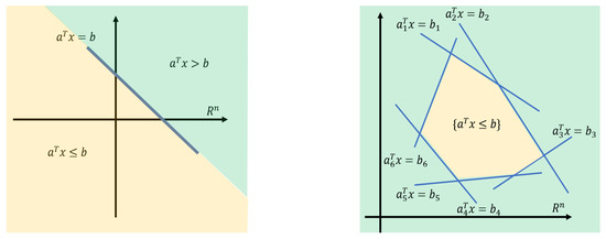
Figure 8.
Green and yellow, respectively, represent a half-space, and the intersection of finite half-spaces forms a polyhedron.
As shown in Figure 9, the distance from the midpoint of the path to the nearest obstacle enables a spherical corridor to be found on the corresponding path segment. Using the contact point between the ball corridor and the obstacle as the tangent point, make a tangent plane tangent to the ball, which separates the ball from a portion of the obstacle. Once this tangent plane is obtained, the obstacles outside the tangent plane are removed to obtain a new radius , a spherical corridor , and a tangent plane , and the above steps are repeated.
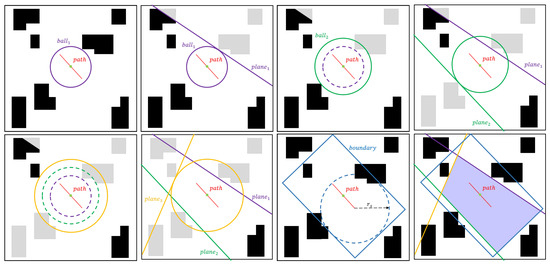
Figure 9.
Continuously expand the spherical corridor, making a tangent plane for each contact point with an obstacle, deleting obstacles outside the tangent plane until it expands to the set boundary, the intersection of the boundary with all tangent planes being the flight corridor of the corresponding path segment.
Since the radius of the ball needs to be calculated several times in the above process, this paper adopts the method in [11] and sets a bounding box to limit the maximum expansion space in the process of finding the ball, in order to reduce the computation time and avoid corridor space search in regions that are too far away. There is also a perceptual boundary for the sensors in the actual flight. The bounding box consists of a cube and its axes are aligned with the path of the corresponding path segment. The minimum distance from each face on the cube to the path segment is . Assuming that the maximum velocity and maximum acceleration of the UAV are and , respectively, the distance of the bounding box should satisfy . The bounding box is set as shown in Figure 9.
In order to make the corridor satisfy the continuity condition, Ref. [11] initializes an ellipsoid containing the two endpoints of the path for expansion, and then continuously iterates over the two parameters of the ellipsoid’s long and short semi-axes. Unlike theirs, our method only needs to iterate one parameter, the radius r of the sphere, then check whether the continuity Formula (5) is satisfied and ensure that all points within the vector are contained within the continuum space of the corridor by inserting intermediate points as shown in Figure 5. The insertion point operation is hardly used in most cases in the experiments.
The pseudo-code of the algorithm for the construction of the flight corridor for convex polyhedra based on the geometric approach is shown in Algorithm 1.
| Algorithm 1 Building Polyhedral Flight Corridor |
|
3.4. Trajectory Optimization
In [9], Wang et al. proposed a method based on the location of the midpoint and the time for the trajectory parameterization of the trajectory class MINCO, which is a class of polynomial trajectories defined as follows:
where , i.e., the coefficients in the polynomial trajectory. Thus, in MINCO, the ith segment trajectory can still be expressed in the following form:
where is the base of the polynomial, is the coefficient matrix, , and .
Ref. [4] models the quadrotor as a non-linear dynamical system that has a flat output of , where denotes the position of the rotor in space and denotes the yaw angle of the rotor. The trajectory planning of the UAV only requires control of the four flat outputs of .
This paper uses MINCO’s trajectory representation method to improve the quality of the trajectory by finding optimal solutions for the constraints. A trajectory segment can thus be expressed as:
Trajectory optimization aims to find a smooth trajectory and to ensure that the trajectory is feasible and safe. In polynomial trajectories, the smoothness of a trajectory can be achieved by controlling the minimum value of its s-order derivative. Trajectory optimization can therefore be formulated in the followingform [12]:
In this paper, we let , i.e., the jerk of the trajectory is minimized under the constraint to ensure the optimality of the trajectory, where is the penalty term on the total time of the trajectory and is the weighting factor for this term. Equation (9a) is the objective function for which the optimization solution is required. Equation (9b) is a constraint on the initial and final states of the trajectory, respectively. and are the matrix forms of the position, velocity, and acceleration of the initial and final states. Equation (9c) indicates that the trajectory corresponding to the ith time passes through the intermediate coordinate point , and M is the total number of path segments. Equation (9d) is a constraint on time. Equation (9e) indicates that the first-order derivative (velocity) as well as the second-order derivative (acceleration) of the trajectory cannot exceed the maximum limit of the UAV dynamics. Equation (9f) represents the safety constraint on the trajectory, which in this paper is set to ensure that all intermediate trajectory points are contained within the flight corridor.
This paper designs cost functions for the feasibility cost corresponding to (9e) and the collision term cost corresponding to (9f), and additionally adds the height cost function; these three cost functions can be expressed as:
where is the collision term cost function, which ensures that the flight trajectory is safe and collision-free. and are limits on the velocity and acceleration, respectively, which the UAV cannot exceed in magnitude during its actual motion in terms of its dynamics. At the same time, this paper aims to minimize the displacement of the UAV in the altitude direction to avoid a collision with obstacles that cannot be perceived above the UAV, so is designed to constrain the change in motion of the trajectory over the flight altitude. and are the weights of the corresponding three cost functions.
A collision term cost function is constructed based on corridor information as:
where is a three-dimensional column vector, denotes the three-dimensional coordinates of a point in space, and is a constant term. This cost function constrains all points on the trajectory to be in half-spaces.
The feasibility cost function is expressed as:
When the velocity and acceleration in the trajectory exceed the maximum limits, a feasibility cost function needs to be imposed. However, since the problem is a soft constraint optimization problem, the velocity and acceleration limits are set to a value slightly smaller than the maximum value of velocity and acceleration allowed by the dynamics. Taking the velocity limit as an example, . Then the velocity penalty term on one dimension is:
and the acceleration penalty term is the same as the velocity penalty term:
For a trajectory constrained at height , this is obtained directly by penalizing the velocity of the trajectory in the height direction by:
where:
4. Experiments
To evaluate the autonomous flight corridor-based obstacle avoidance algorithm proposed in this paper, we first verified the path planning algorithm with height limitation. Then, we verified the superiority of the polyhedral corridor using MATLAB simulations and the flight corridor-based simulation experiments in the ROS environment. A further obstacle avoidance experiment using a real UAV was completed with an outdoor flight.
4.1. Path Planning Simulation Experiments
In order to verify that the algorithm limits the variation in 3D height, this paper verifies the effectiveness of the algorithm in different 3D maps, as shown in Figure 10. In the figure, both algorithms have the same start and end points, the paths solved by the algorithm in this paper are shown in red, and the paths solved by the JPS algorithm are shown in black.
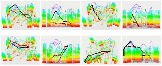
Figure 10.
We compared the height changes of our algorithm and JPS algorithm in path planning in 3D maps. The settings for the starting and ending points in the map are the same, with black being the curve calculated by the JPS algorithm and red being the curve calculated by our method.
When comparing the size of the total height changes of the paths obtained by the two algorithms in the same map, as shown in Table 1, the height changes of the algorithms in this paper are all smaller than the height changes of the JPS algorithm, justifying the restriction on the height changes of the paths by this method.

Table 1.
Comparison of JPS and this paper’s algorithm height variation in 3D maps.
4.2. Flight Corridor Construction Algorithm Simulation Experiments
Figure 11 shows the construction results of spherical corridors, cubic corridors, and polyhedral corridors under six different maps (with each column having the same map and path). From the graph, it can intuitively be seen that the spatial occupancy rates of the three corridors are in order: polyhedral corridor>cubic corridor>spherical corridor.
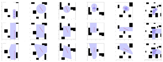
Figure 11.
Comparison of flight corridor construction methods. Each horizontal row represents a different map, and each vertical row has identical maps and paths, in order to compare the computational time and spatial size of the three corridor generation methods.
This paper counts the time consumed to build a corridor using MATLAB in the same obstacle environment and the space occupation of the corridor (expressed as area size in two dimensions) with a computer hardware configuration of Intel i7. The results are shown in Table 2 and Table 3.
Table 2.
Comparison of calculation times for the three corridors (ms).
Table 3.
Comparison of space utilization of three types of corridor (m2).
In Table 2, the cubic corridor construction consumes more computational time than the other two construction methods because the cube corridor takes a lot of computational resources to retrieve whether the cube will encounter an obstacle after each outward extension of its face. In most cases, the computational time for the polyhedral corridor is greater than that for the spherical corridor due to the fact that its expansion does not stop after the first obstacle it encounters. Thus, in principle, the polyhedral corridor construction takes more time. In maps 1 and 6, however, the spherical corridor takes more time because of the introduction of the insertion of points.
As can be seen from Table 3, the polyhedral corridors take up far more space than the spherical and cubic corridors in most cases. In Map 6, the cube corridor occupies more space than the polyhedron because the obstacles around the paths in that map can be separated by the use of exactly two cubes, and the axes of the cubes and the placement of the obstacles are in the same direction.
4.3. ROS-Based Flight Obstacle Avoidance Simulation Experiments
This paper uses Gazebo to build the simulation system environment. Gazebo integrates a large library of sensor models, including IMU, GPS, barometer, camera, etc., which are commonly used for quadcopter UAVs, and can add its physical properties to objects, such as gravity, wind speed, light, etc., which facilitates the deployment of simulation experiments into real environments. This paper uses a simulation drone [22], as shown in Figure 12.
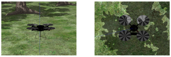
Figure 12.
Main view and top view of the simulation system UAV. The left figure is the main view and the right figure is the top view.
The simulation experiment scenario uses both indoor as well as wooded simulation environments [23], as shown in Figure 13.
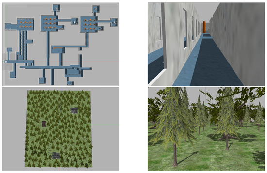
Figure 13.
Indoor and wooded simulation environments.
In this paper, simulation experiments of the algorithm based on flying corridors are conducted based on indoor corridors and outdoor wooded scenes, respectively, as shown in Figure 14.
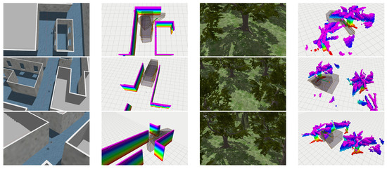
Figure 14.
Flight corridor-based simulation experiments in two different environments.
4.4. Physical Flight Experiments
The actual UAV built for the experiments in this paper is shown in Figure 15, with a wheelbase of 250 mm in length, a height of 158 mm, and a weight of 1.09 kg (without battery).
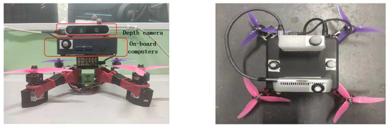
Figure 15.
Physical drone hardware configuration.
The UAV uses CUAV’s CUAV-nora+ flight control module, which has high stability, accurate inertial measurement devices, and a high and stable barometer setting. The environmental awareness, motion planning, and flight control modules run on the Intel NUC-i7 computer, which is an x86 architecture. The Realsense D435i depth camera from Intel was used in this paper. This depth camera has the advantages of a compact size and low energy consumption, and its effective distance measurement is 10 m, which meets the experimental requirements. The USB-C*3.1 interface is used to support fast data transfer.
In the indoor experiments, the VICON system was used to achieve the positioning of the UAV. In the outdoor experiments, VINS was used to achieve UAV positioning. The flight avoidance process is shown in Figure 16.
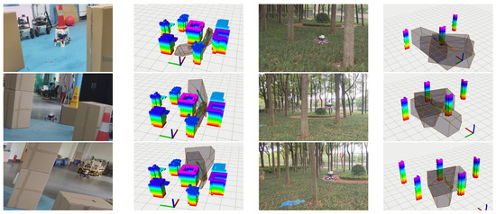
Figure 16.
Flight corridor-based obstacle avoidance experiments in indoor and wooded environments.
The trajectory of the aircraft in the indoor as well as outdoor experiments for obstacle avoidance is shown in Figure 17.

Figure 17.
Indoorand outdoor flight test data. The left figure shows the trajectory curve, the center shows the velocity curve, and the right figure shows the attitude angle curve.
Combining the above experiments, the algorithm proposed in this paper can achieve autonomous obstacle avoidance in complex low-altitude environments.
5. Conclusions
In this paper, the construction method of safe flight corridors for UAVs and the autonomous obstacle avoidance method for UAVs based on the flight corridor are studied, and are used to realize the online solution of UAVs’ efficient real-time trajectory and ensure flight safety, and provide certain theoretical and experimental bases for the development of UAV autonomous obstacle avoidance technology. The proposed corridor construction algorithm reduces the time required to construct the corridor while ensuring the space utilization of the corridor compared to previous methods. The corridor-based autonomous obstacle avoidance algorithm proposed in this paper effectively reduces the height output of path planning and successfully achieves autonomous obstacle avoidance in indoor and wooded environments. To provide further perspectives on the paper, research can be carried out using flight corridors to target the obstacle avoidance problem for dynamic obstacles, as well as the obstacle avoidance problem for swarming UAVs.
Author Contributions
Conceptualization, Y.L.; methodology, Y.N. and Z.M.; validation, Z.W.; software. A.M. All authors have read and agreed to the published version of the manuscript.
Funding
This paper was supported by National Natural Science Foundation of China (No. 61876187, 62303481) and Natural Science Foundation of Hunan Province (No. S2022JJQNJJ2084).
Data Availability Statement
Restrictions apply to the availability of these data.
Conflicts of Interest
The authors declare no conflict of interest. The funders had no role in the design of the study; in the collection, analyses, or interpretation of data; in the writing of the manuscript; or in the decision to publish the results.
References
- Kakaletsis, E.; Symeonidis, C.; Tzelepi, M.; Mademlis, I.; Tefas, A.; Nikolaidis, N.; Pitas, I. Computer Vision for Autonomous UAV Flight Safety: An Overview and a Vision-based Safe Landing Pipeline Example. ACM Comput. Surv. (CSUR) 2021, 54, 1–37. [Google Scholar] [CrossRef]
- Gupta, P.; Pareek, B.; Singal, G.; Rao, D.V. Edge Device Based Military Vehicle Detection and Classification from UAV. Multimed. Tools Appl. 2021, 81, 19813–19834. [Google Scholar] [CrossRef]
- Teulière, C.; Marchand, E.; Eck, L. 3-D Model-Based Tracking for UAV Indoor Localization. IEEE Trans. Cybern. 2015, 45, 869–879. [Google Scholar] [CrossRef] [PubMed]
- Mellinger, D.; Kumar, V. Minimum Snap Trajectory Generation and Control for Quadrotors. In Proceedings of the 2011 IEEE International Conference on Robotics and Automation, Shanghai, China, 9–13 May 2011; pp. 2520–2525. [Google Scholar]
- Usenko, V.C.; von Stumberg, L.; Pangercic, A.; Cremers, D. Real-time Trajectory Replanning for MAVs Using Uniform B-splines and a 3D Circular Buffer. In Proceedings of the International Conference on Intelligent Robots and Systems (IROS), Vancouver, BC, Canada, 24–28 September 2017; pp. 215–222. [Google Scholar]
- Zhou, B.; Gao, F.; Wang, L.; Liu, C.; Shen, S. Robust and Efficient Quadrotor Trajectory Generation for Fast Autonomous Flight. IEEE Robot. Autom. Lett. 2019, 4, 3529–3536. [Google Scholar] [CrossRef]
- Zhou, X.; Wang, Z.; Ye, H.; Xu, C.; Gao, F. EGO-Planner: An ESDF-Free Gradient-Based Local Planner for Quadrotors. IEEE Robot. Autom. Lett. 2021, 6, 478–485. [Google Scholar] [CrossRef]
- Zhou, X.; Wen, X.; Wang, Z.; Gao, Y.; Li, H.; Wang, Q.; Yang, T.; Lu, H.; Cao, Y.; Xu, C.; et al. Swarm of Micro Flying Robots in the Wild. Sci. Robot. 2022, 7, 1–21. [Google Scholar] [CrossRef] [PubMed]
- Wang, Z.; Zhou, X.; Xu, C.; Gao, F. Geometrically Constrained Trajectory Optimization for Multicopters. IEEE Trans. Robot. 2021, 38, 3259–3278. [Google Scholar] [CrossRef]
- Gao, F.; Wang, L.; Zhou, B.; Zhou, X.; Pan, J.; Shen, S. Teach-Repeat-Replan: A Complete and Robust System for Aggressive Flight in Complex Environments. IEEE Trans. Robot. 2020, 36, 1526–1545. [Google Scholar] [CrossRef]
- Liu, S.; Watterson, M.; Mohta, K.; Sun, K.; Bhattacharya, S.; Taylor, C.J.; Kumar, V.R. Planning Dynamically Feasible Trajectories for Quadrotors Using Safe Flight Corridors in 3-D Complex Environments. IEEE Robot. Autom. Lett. 2017, 2, 1688–1695. [Google Scholar] [CrossRef]
- Ren, Y.; Zhu, F.; Liu, W.; Wang, Z.; Lin, Y.; Gao, F.; Zhang, F. Bubble Planner: Planning High-speed Smooth Quadrotor Trajectories using Receding Corridors. In Proceedings of the 2022 IEEE/RSJ International Conference on Intelligent Robots and Systems (IROS), 2022, IEEE International Conference on Intelligent Robots and Systems, Kyoto, Japan, 23–27 October 2022; pp. 6332–6339. [Google Scholar]
- Gao, F.; Shen, S. Online Quadrotor Trajectory Generation and Autonomous Navigation on Point Clouds. In Proceedings of the 2016 IEEE International Symposium on Safety, Security, and Rescue Robotics (SSRR), Lausanne, Switzerland, 23–27 October 2016; pp. 139–146. [Google Scholar]
- Ji, J.; Wang, Z.; Wang, Y.; Xu, C.; Gao, F. Mapless-Planner: A Robust and Fast Planning Framework for Aggressive Autonomous Flight without Map Fusion. In Proceedings of the 2021 IEEE International Conference on Robotics and Automation (ICRA), Xi’an, China, 30 May–5 June 2021; pp. 6315–6321. [Google Scholar]
- Florence, P.R.; Carter, J.; Ware, J.A.; Tedrake, R. NanoMap: Fast, Uncertainty-Aware Proximity Queries with Lazy Search Over Local 3D Data. In Proceedings of the 2018 IEEE International Conference on Robotics and Automation (ICRA), Brisbane, Australia, 21–25 May 2018; pp. 7631–7638. [Google Scholar]
- Chen, J.; Liu, T.; Shen, S. Online Generation of Collision-free Trajectories for Quadrotor Flight in Unknown Cluttered Environments. In Proceedings of the 2016 IEEE International Conference on Robotics and Automation (ICRA), Stockholm, Sweden, 16–21 May 2016; pp. 1476–1483. [Google Scholar]
- Gao, F.; Wu, W.; Lin, Y.; Shen, S. Online Safe Trajectory Generation for Quadrotors Using Fast Marching Method and Bernstein Basis Polynomial. In Proceedings of the 2018 IEEE International Conference on Robotics and Automation (ICRA), Brisbane, Australia, 21–25 May 2018; pp. 344–351. [Google Scholar]
- Kala, R.; Shukla, A.; Tiwari, R. Fusion of Probabilistic A* Algorithm and Fuzzy Inference System for Robotic Path Planning. Artif. Intell. Rev. 2010, 33, 307–327. [Google Scholar] [CrossRef]
- Yao, J.; Lin, C.; Xie, X.; Wang, A.J.A.; Hung, C.C. Path Planning for Virtual Human Motion Using Improved A* Star Algorithm. In Proceedings of the 2010 Seventh International Conference on Information Technology: New Generations, Las Vegas, NV, USA, 12–14 April 2010; pp. 1154–1158. [Google Scholar]
- Klemm, S.; Oberlaender, J.; Hermann, A.; Roennau, A.; Schamm, T.; Zoellner, J.M.; Dillmann, R. RRT*-Connect: Faster, Asymptotically Optimal Motion Planning. In Proceedings of the 2015 IEEE International Conference on Robotics and Biomimetics (ROBIO), Zhuhai, China, 6–9 December 2015; pp. 1670–1677. [Google Scholar]
- Kavraki, L.E.; Svestka, P.; Latombe, J.C.; Overmars, M.H. Probabilistic Roadmaps for Path Planning in High-dimensional Configuration Spaces. IEEE Trans. Robot. Autom. 1996, 12, 566–580. [Google Scholar] [CrossRef]
- Tordesillas, J.; Lopez, B.T.; Everett, M.; How, J.P. FASTER: Fast and Safe Trajectory Planner for Navigation in Unknown Environments. IEEE Trans. Robot. 2022, 38, 922–938. [Google Scholar] [CrossRef]
- Cao, C.; Zhu, H.; Cho, H.; Zhang, J. Exploring Large and Complex Environments Fast and Efficiently. In Proceedings of the 2021 IEEE International Conference on Robotics and Automation (ICRA), Xi’an, China, 30 May–5 June 2021; pp. 7781–7787. [Google Scholar]
Disclaimer/Publisher’s Note: The statements, opinions and data contained in all publications are solely those of the individual author(s) and contributor(s) and not of MDPI and/or the editor(s). MDPI and/or the editor(s) disclaim responsibility for any injury to people or property resulting from any ideas, methods, instructions or products referred to in the content. |
© 2023 by the authors. Licensee MDPI, Basel, Switzerland. This article is an open access article distributed under the terms and conditions of the Creative Commons Attribution (CC BY) license (https://creativecommons.org/licenses/by/4.0/).