Drone-Assisted Fingerprint Localization Based on Kernel Global Locally Preserving Projection

Abstract

To improve the limited number of fixed access points (APs) and the inability to dynamically adjust them in fingerprint localization, this paper attempted to use drones to replace these APs. Drones have higher flexibility and accuracy, can hover in different locations, and can adapt to different scenarios and user needs, thereby improving localization accuracy. When performing fingerprint localization, it is often necessary to consider various factors such as environmental complexity, large-scale raw data collection, and signal strength variation. These factors can lead to high-dimensional and complex nonlinear relationships in location fingerprints, thereby greatly affecting localization accuracy. In order to overcome these problems, this paper proposes a kernel global locally preserving projection (KGLPP) algorithm. The algorithm can reduce the dimensionality of location fingerprint data while preserving its most-important structural information, and it combines global and local information to avoid the problem of reduced information and poor dimensionality reduction effects, which may arise from considering only one. In the process of location estimation, an improved weighted k-nearest neighbor (IWKNN) algorithm is adopted to more accurately estimate the target’s position. Unlike the traditional KNN or WKNN algorithms, the IWKNN algorithm can choose the optimal number of nearest neighbors autonomously, perform location estimation and weight calculation based on the actual situation, and thus, obtain more-accurate location estimation results. The experimental results showed that the algorithm outperformed other algorithms in terms of both the average error and localization accuracy.

1. Introduction

With the emergence of unmanned aerial vehicles (UAVs), they are widely used to establish wireless communication networks, utilizing their characteristics of flying in the air to provide relatively stable and reliable communication services [1,2,3]. Due to their high efficiency, low cost, and wide deployment potential, particularly in achieving the next-generation mobile communication standards, UAVs have come to play a dominant role [4]. This not only requires strict compliance with the necessary conditions for communication by network technology, but also requires conceptual processing to ensure excellent performance and the promotion of the application of unmanned aerial vehicles in 5G networks [5]. In the future, we can expect to use unmanned aerial vehicles extensively in various human activity domains and leverage their capabilities for diverse intelligent applications. These applications may include, but are not limited to search and rescue, environmental monitoring, agricultural management, logistics delivery, and so on. It is expected that, with the development of unmanned aerial vehicle technology and the increase in application scenarios, we will enter an era of drone-assisted networks [6].

In recent years, the broadband communication industry has achieved rapid development, including various types of fixed and mobile broadband communications, which can be seen globally. However, not all areas have full coverage of broadband communication, especially in some remote or mountainous areas. In the event of accidents in these areas, it is difficult to accurately locate them, so drones can play a role in this situation, replacing traditional fixed APs and solving the problem of zero-point coverage. In [7], the researchers proposed a new UAV localization method that uses ultra-wideband radio signals as localization signals and can effectively improve the localization performance in non-line-of-sight situations by applying the correction values of ray-tracing algorithms to ultra-wideband ranging data. However, this approach requires the deployment of multiple positioning base stations to collect enough signal data to enable the positioning of the UAV. As a result, the cost of deploying base stations increases accordingly. The work [8] proposed indoor positioning of UAVs using WiFi signal ranging. However, this method needs to obtain the exact location of each AP in advance to achieve distance-based WiFi localization. This further increases the difficulty and complexity of UAV positioning. A new method for indoor UAV localization was proposed in [9], which utilizes camera optical flow data and inertial sensor information for fusion. However, the method requires processing a large amount of image information in visual localization, which puts higher demands on the computing power of computers, and general computers are unable to perform such high-intensity operations, resulting in high energy consumption and low real-time performance.

With the rapid development of technology, the demand for positioning technology on mobile terminals has also increased. Mobile-terminal-positioning technology has become a very important research area in the applications of the Internet of Things and device-to-device communication [10,11]. In the Internet of Things (IoT), communication and collaboration between devices are crucial [12]. To ensure effective interaction and resource utilization, location information is essential. The location information of mobile terminals enables the quick establishment of direct communication links and facilitates resource sharing. Whether indoors or outdoors, the location information of mobile terminals is necessary. GPS and base station positioning technologies meet outdoor positioning needs, but people spend most of their time indoors. However, in indoor environments, buildings obstruct signals, resulting in rapid attenuation or even complete unavailability of GNSS signals, which cannot fulfill the indoor navigation and positioning requirements [13]. In indoor positioning, better performance can be obtained by using WiFi [14], Bluetooth [15], RFID [16], ultrasound technology [17], frequency modulation broadcasting [18], infrared technology, and other positioning technologies. Among the above methods, WiFi positioning technology has a wide infrastructure and is easy to deploy, so WiFi-based positioning technology is widely used for indoor positioning [19,20,21,22]. Fingerprint positioning, as a WiFi-signal-based indoor positioning technology, has received widespread attention in recent years due to its high accuracy, low cost, and easy implementation.

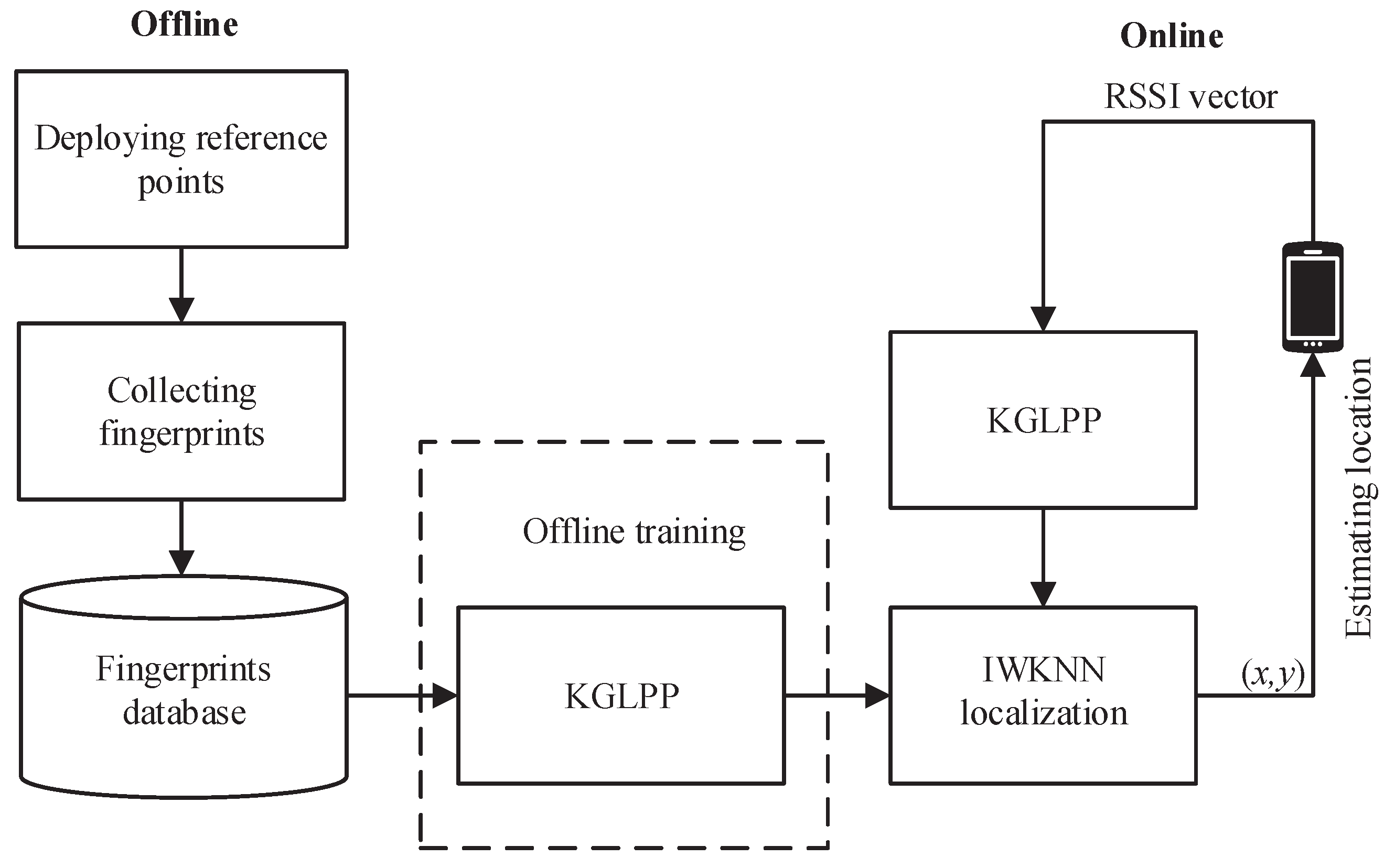
The WLAN-based RSSI positioning fingerprint algorithm is mainly divided into offline and online phases [23,24]. In the offline phase, the first step is to deploy some reference points in the positioning area and record the WiFi signal strength indicator (RSSI) values at each reference point. Data collection can be performed by placing specific access points (APs) at certain locations inside the building. Then, at each known location, mobile devices are used to scan and record the RSSI values between each AP. Next, the collected fingerprint data are processed and stored. The processing involves preprocessing of the signal strength indicator, such as removing outliers, smoothing, etc. Then, the processed fingerprint data are stored in a database for subsequent positioning queries. In the online phase, when a mobile device needs to be located, it scans for available APs in the vicinity and obtains the RSSI values at the current location. Then, these real-time measured RSSI values are compared and matched with the stored fingerprint database from the offline phase. Typically, matching algorithms such as the k-nearest neighbor algorithm are used to find the best-matching fingerprint set, thereby determining the location of the mobile device.

In order to solve the problem of the indoor environment being able to affect the localization, researchers have proposed various preprocessing methods for fingerprint data, aiming to reduce the influence of the indoor environment on the fingerprint database and avoid the influence of outliers and noise on the fingerprint database, so as to improve the accuracy of building thefingerprint database. Li et al. proposed a KPCA-based indoor localization method [25], which hinges on mapping data from the original space to a high-dimensional feature space using nonlinear mapping, followed by linear principal component analysis (PCA). To better handle nonlinear transformations, KPCA introduces the kernel function trick, which replaces the dot product between data vectors in the feature space [26] with a similarity measure calculated by the kernel function. However, despite its commitment to capturing the nonlinear features of the data by introducing kernel functions, the algorithm used by KPCA suffers from the same shortcomings as PCA. That is, only the global Euclidean structure (or global variance) of the data is preserved, while the local neighborhood structure of the data is ignored. This global nature makes it difficult for KPCA to completely capture the complex relationships and local features between the data, resulting in its poor performance in some cases.

He et al. used the locally preserving projection (LPP) method to reduce the dimensionality of the original data and used KLPP as the kernel function expansion method for LPP [27]. Compared with PCA and KPCA, the design ideas of LPP and KLPP focus on retaining the local structural information of the data while ignoring the global data structure, and this design idea may lead to a certain loss of data variance [28]. In performing data dimensionality reduction, the LPP and KLPP methods focus on preserving the local structural information of the data. This approach may result in a distorted global data structure, and the data points are restricted to a very small area [29]. This is because these methods do not properly restrict the projection distance between non-adjacent data points, which leads to unsatisfactory processing of the algorithm for large datasets. To obtain a reliable feature representation, we must take into account the global and local structure of the dataset and perform dimensionality reduction using appropriate processing. In recent research on data dimensionality reduction, some scholars have combined the PCA and LPP algorithms to be able to preserve both global and local data structures in low-dimensional spaces [28,29,30,31]. In the process of studying the combination of PCA and LPP, a technique proposed by the scholar Luo [31], namely the global locally preserving projection (GLPP) method, successfully integrates two dimensionality-reduction methods, PCA and LPP, under the same framework. After experimental validation, the GLPP method can better maintain the global and local characteristics of the data and combine the advantages of both, while avoiding the effects of problems such as principal component rotation and no samples in the neighborhood.

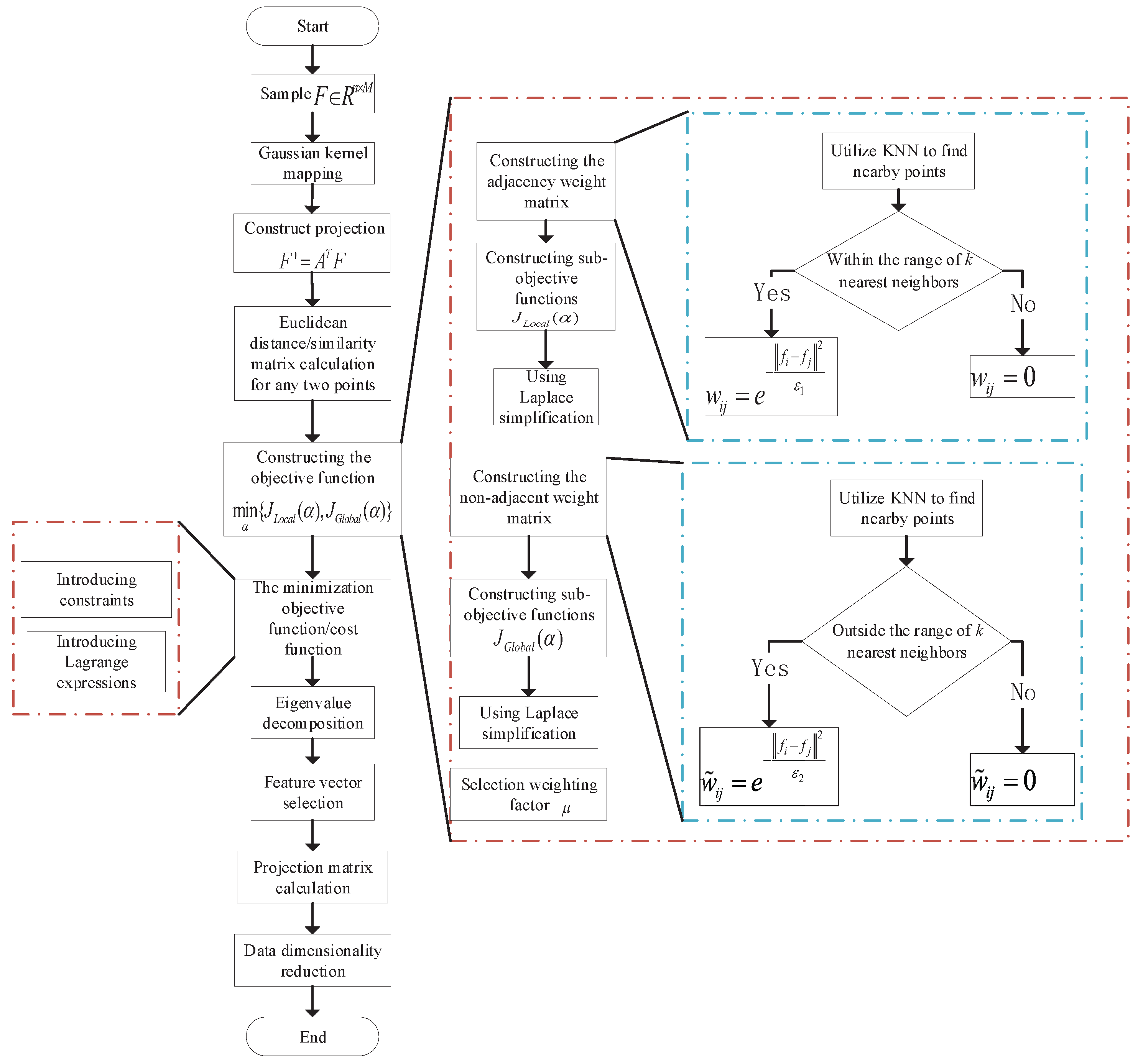
This paper proposes a novel nonlinear dimensionality-reduction method, called kernel global locally preserving projection (KGLPP). The proposed method is an extension and improvement of the global locally preserving projection (GLPP) algorithm, which employs kernel techniques to map and process data for better preservation of the global and local structure of the dataset. Compared to other dimensionality-reduction methods, KGLPP offers significant advantages in reducing data redundancy, improving the accuracy and reliability of feature selection. It is shown that we can obtain KPCA and KLPP methods through the derivation of KGLPP. Both methods are the basis laid by KGLPP [32] and can be considered as a special case of KGLPP. Based on this, KGLPP-based drone-assisted fingerprint localization is proposed. The connection between the KGLPP algorithm and the drone AP solution is as follows: (1) In the drone AP solution, drones are used as carriers for APs, allowing them to freely move and adjust their positions within indoor environments. (2) In this scenario, the KGLPP algorithm can be used to process the fingerprint data collected from drone APs. It can reduce the high-dimensional fingerprint data to a lower dimension, thereby reducing computational complexity and extracting the key features of the data. (3) The KGLPP algorithm computes based on the similarity matrix of fingerprint data, which is obtained through the collection by the drone APs. (4) By using the KGLPP algorithm for dimensionality reduction, we can effectively analyze and process the data collected by the drone APs while preserving the local relationships and global structure of the fingerprint data.

We applied the KGLPP algorithm to both the offline and online training phases of fingerprint data to improve the accuracy and efficiency of fingerprint localization. In the online phase of fingerprint localization, an improved weighted k-nearest neighbor (IWKNN) algorithm was used for position estimation. Compared the with traditional k-nearest neighbor algorithms, the IWKNN algorithm can adaptively select the required number of fingerprints for location based on the needs and weight them according to the distance and similarity of the fingerprint information, thus achieving more-accurate and -reliable fingerprint position prediction. Therefore, combining the use of the KGLPP algorithm and IWKNN algorithm can effectively help us process fingerprint data and significantly improve the accuracy of fingerprint localization. The experimental results showed that the algorithm proposed in this paper was significantly better than several other fingerprint-localization algorithms. In summary, our contributions are as follows:

• Using drones to replace APs for localization is a new approach that has several advantages compared to the traditional AP method. Drones can maneuver freely and obtain comprehensive information, with relatively low requirements for application scenarios. Its hovering function and built-in sensors can provide more-accurate data; with a low cost and rapid response, it is suitable for various practical application scenarios.
• In this study, we propose a novel fingerprint-localization algorithm based on kernel global locally preserving projection (KGLPP). The algorithm was trained using both an offline fingerprint database and online fingerprint vectors. The KGLPP method improves localization accuracy by combining global and local features, and its kernel-based feature extraction exhibits powerful nonlinear mapping capabilities, making it suitable for complex environments. The method also reduces computational complexity and provides the real-time performance and responsiveness required for practical applications. Furthermore, the KGLPP method exhibits robustness to interference and changes in actual environments, thereby improving the accuracy and stability of fingerprint-based positioning.
• In the localization process, an improved weighted k-nearest neighbor (IWKNN) algorithm is used. This algorithm introduces a cumulative contribution parameter and limits its range between 0 and 1, allowing it to adaptively select the required number of nearest neighbors, thus avoiding the overfitting or underfitting problems that may occur when directly specifying the k value and improving the accuracy of the algorithm.

The organizational structure of this paper is as follows. In Section 2, we review some background techniques on the KGLPP algorithm. In Section 3, we introduce the system framework. In Section 4, the details of the algorithm are introduced. The explanatory results of the simulation and experiment are provided in Section 5. The paper is concluded in Section 6.

2. Background Techniques

2.1. Kernel Principal Component Analysis

Kernel principal component analysis (KPCA) is a nonlinear form of PCA [25]. The KPCA method is based on the nonlinear mapping function $\varphi$; here, the kernel method was used to map the original space to the feature space, and PCA was performed on the feature space. Let the nonlinear transformation function $\varphi$ be used as a mapping function to transform the data in the original location fingerprint space $\mathit{F}=({\mathit{f}}_1,{\mathit{f}}_2,\cdots ,{\mathit{f}}_M)\in {\mathit{R}}^{n\times M}$ into a new feature space. Therefore, we mapped ${\mathit{f}}_1,{\mathit{f}}_2,\cdots ,{\mathit{f}}_M$ to the new feature space according to this mapping function, so that, in this new feature space, ${\mathit{f}}_1,{\mathit{f}}_2,\cdots ,{\mathit{f}}_M$ are represented as $\varphi \left({\mathit{f}}_1\right),\varphi \left({\mathit{f}}_2\right),\cdots ,\varphi \left({\mathit{f}}_M\right)$, respectively. This feature space is defined by the function $\varphi \left(\mathit{F}\right)$. In addition, it was assumed that the sample data in this feature space were preprocessed to be centered (i.e., their average was adjusted to zero), which means that the condition in Equation (1) is satisfied.

$$\sum _{j=1}^M\varphi \left({\mathit{f}}_j\right)=0$$

(1)

By computing Equation (2), we can obtain the covariance matrix $\mathit{C}$ in the feature space.

$$\mathit{C}=\frac{1}{M}\varphi \left(\mathit{F}\right){\varphi }^T\left(\mathit{F}\right)=\frac{1}{M}\sum _{j=1}^M\varphi \left({\mathit{f}}_j\right){\varphi }^T\left({\mathit{f}}_j\right)$$

(2)

Based on the expression in Equation (3), we can obtain the eigenvalues $\lambda$ and corresponding eigenvectors $\mathit{V}$ of the covariance matrix $\mathit{C}$.

$$\mathit{CV}=\lambda \mathit{V}$$

(3)

During the process of eigendecomposition, the obtained eigenvector $\mathit{V}$ belongs to the space generated by $\varphi \left({\mathit{f}}_1\right),\varphi \left({\mathit{f}}_2\right),\cdots ,\varphi \left({\mathit{f}}_M\right)$. This means that the eigenvector $\mathit{V}$ can be seen as a vector in the linear space spanned by $\varphi \left(\mathit{F}\right)$, and the dimension of this space depends on the number of dimensions obtained after applying the mapping function $\varphi \left(\mathit{F}\right)$ to the original dataset $\mathit{F}$. In addition, in this feature space spanned by $\varphi \left(\mathit{F}\right)$, any eigenvector can be seen as a linear combination of $\varphi \left(\mathit{F}\right)$, and the entire process can be expressed using Equation (4).

$$\mathit{V}=\sum _{j=1}^M{\mathit{\alpha }}_j\varphi \left({\mathit{f}}_j\right)=\mathit{\alpha }\varphi \left(\mathit{F}\right)$$

(4)

where ${\mathit{\alpha }}_j$ is a coefficient vector of the same order as $\varphi \left({\mathit{f}}_j\right)$, and by substituting Equations (2) and (4) into Equation (3), we obtain

$$\frac{1}{M}\varphi \left(\mathit{F}\right){\varphi }^T\left(\mathit{F}\right)\varphi \left(\mathit{F}\right)\mathit{\alpha }=\lambda \varphi \left(\mathit{F}\right)\mathit{\alpha }$$

(5)

Multiplying ${\varphi }^T\left(\mathit{F}\right)$ at the left of both sides in Equation (5) yields

$$\frac{1}{M}{\varphi }^T\left(\mathit{F}\right)\varphi \left(\mathit{F}\right){\varphi }^T\left(\mathit{F}\right)\varphi \left(\mathit{F}\right)\mathit{\alpha }=\lambda {\varphi }^T\left(\mathit{F}\right)\varphi \left(\mathit{F}\right)\mathit{\alpha }$$

(6)

Defining a kernel matrix $\mathit{K}\in {\mathit{R}}^{M\times M}$ with ${\mathit{K}}_{ij}=\mathit{k}({\mathit{f}}_i,{\mathit{f}}_j)=\varphi \left({\mathit{f}}_i\right)·\varphi \left({\mathit{f}}_j\right)={\varphi }^T\left({\mathit{f}}_i\right)\varphi \left({\mathit{f}}_j\right)$, therefore, Equation (6) can be simplified as

$$M\lambda \mathit{K}\mathit{\alpha }=\mathit{KK}\mathit{\alpha }\Rightarrow \tilde{\lambda }\mathit{\alpha }=\mathit{K}\mathit{\alpha }$$

(7)

From Equation (7), it can be seen that obtaining the eigenvalues and eigenvectors of matrix $\mathit{K}$ is a crucial step in SVM, as this process directly leads to the eigenvalues and corresponding eigenvectors of $\mathit{S}$. Assuming that the matrix $\mathit{K}$ has M eigenvectors and corresponding eigenvalues, we can perform dimensionality reduction from a high-dimensional space to a low-dimensional space by only considering the l($l\le M$) largest eigenvalues ${\tilde{\lambda }}_1\ge {\tilde{\lambda }}_2\ge \cdots {\tilde{\lambda }}_{l-1}\ge {\tilde{\lambda }}_l$ of $\mathit{K}$ and their corresponding l unit-orthogonalized eigenvectors $\mathit{\alpha }={[{\mathit{\alpha }}_1,{\mathit{\alpha }}_2,\cdots ,{\mathit{\alpha }}_l]}^T$. The feature extraction of feature space $\varphi \left(\mathit{F}\right)$ is performed to calculate the projection from $\varphi \left(\mathit{F}\right)$ to the feature vector space. The jth sample is projected to the kth coordinate axis ${\mathit{V}}_k$, as shown in Equation (8).

$$\begin{array}{cc}\hfill {\mathit{t}}_{kj}=& {\varphi }^T\left({\mathit{f}}_j\right){\mathit{V}}_k\hfill \\ \hfill & ={\varphi }^T\left({\mathit{f}}_j\right)\sum _{i=1}^N{\mathit{\alpha }}_{ki}\varphi \left({\mathit{f}}_i\right)\hfill \\ \hfill & =\sum _{i=1}^N{\mathit{\alpha }}_{ki}{\varphi }^T\left({\mathit{f}}_j\right)\varphi \left({\mathit{f}}_i\right)\hfill \end{array}$$

(8)

2.2. Kernel Locally Preserving Projection

The kernel locally preserving projection (KLPP) algorithm is a nonlinear extension of the locally preserving projection (LPP) [27] algorithm. KLPP utilizes kernel functions to perform nonlinear mapping on data, effectively taking into account the nonlinear structure that exists within the dataset and greatly improving dimensionality reduction performance. For a given dataset $\mathit{F}={({\mathit{f}}_1,{\mathit{f}}_2,\cdots ,{\mathit{f}}_M)}^T$, KLPP first applies a nonlinear mapping function $\varphi (·)$ to map the original data to a feature space, allowing effective data processing in a low-dimensional space. Then, the KLPP algorithm performs a linear locally preserving projection (LPP) procedure on the dataset $\varphi \left(\mathit{F}\right)={(\varphi \left({\mathit{f}}_1\right),\varphi \left({\mathit{f}}_2\right),\cdots ,\varphi \left({\mathit{f}}_M\right))}^T$, retaining only the most-important features of the dataset. The KLPP eigenvector problem can be represented as [31]

$$\varphi \left(\mathit{F}\right)\mathit{Q}{\varphi }^T\left(\mathit{F}\right)\mathit{V}=\lambda \varphi \left(\mathit{F}\right)\mathit{D}{\varphi }^T\left(\mathit{F}\right)\mathit{V}$$

(9)

where $\mathit{Q}=\mathit{D}-\mathit{W}$ is a Laplacian matrix. $\mathit{W}$ is a symmetric weight matrix representing the connection strength between each node in a graph or network. $\mathit{D}$ is a diagonal matrix where each diagonal element ${\mathit{d}}_{ii}={\sum }_{j=1}{\mathit{w}}_{ij}$ represents the degree of each node. For each element ${\mathit{w}}_{ij}$ in matrix $\mathit{W}$, it represents the connection weight between sample points ${\mathit{f}}_{\mathit{i}}$ and ${\mathit{f}}_{\mathit{j}}$. If ${\mathit{f}}_{\mathit{i}}$ and ${\mathit{f}}_{\mathit{j}}$ are adjacent and connected, then ${\mathit{w}}_{ij}$ is not equal to 0; otherwise, ${\mathit{w}}_{ij}$ is equal to 0. For a more-detailed definition of matrix $\mathit{W}$, please refer to [30]. This method is similar to KPCA, representing feature vectors in the dataset as $\mathit{V}={\sum }_{i=1}^M{\mathit{\alpha }}_i\varphi \left({\mathit{f}}_i\right)=\mathit{\alpha }\varphi \left(\mathit{F}\right)$, where $\varphi \left({\mathit{f}}_i\right)$ is the mapping function corresponding to sample point ${\mathit{f}}_{\mathit{i}}$ in the original space. Meanwhile, the kernel matrix $\mathit{K}\in {\mathit{R}}^{M\times M}$ is defined, where each element ${\mathit{k}}_{ij}=\mathit{k}({\mathit{f}}_i,{\mathit{f}}_j)=\varphi \left({\mathit{f}}_i\right)·\varphi \left({\mathit{f}}_j\right)={\varphi }^T\left({\mathit{f}}_i\right)\varphi \left({\mathit{f}}_j\right)$ represents the value of the kernel function between sample points ${\mathit{f}}_{\mathit{i}}$ and ${\mathit{f}}_{\mathit{j}}$, and multiplying ${\varphi }^T\left(\mathit{F}\right)$ at the left of both sides in Equation (9) yields

$${\varphi }^T\left(\mathit{F}\right)\varphi \left(\mathit{F}\right)\mathit{Q}{\varphi }^T\left(\mathit{F}\right)\varphi \left(\mathit{F}\right)\mathit{\alpha }={\varphi }^T\left(\mathit{F}\right)\lambda \varphi \left(\mathit{F}\right)\mathit{D}{\varphi }^T\left(\mathit{F}\right)\varphi \left(\mathit{F}\right)\mathit{\alpha }.$$

(10)

Equation (10) can be simplified and re-expressed by Equation (11):

$$\mathit{KQK}\mathit{\alpha }=\lambda \mathit{K}\mathit{DK}\mathit{\alpha }$$

(11)

Assume the eigenvectors of Equation (11) are ${\mathit{\alpha }}_1,{\mathit{\alpha }}_2,\cdots ,{\mathit{\alpha }}_M$. The jth sample is projected to the kth coordinate axis ${\mathit{V}}_k$, as shown in Equation (12).

$$\begin{array}{cc}\hfill {\mathit{t}}_{kj}& ={\varphi }^T\left({\mathit{f}}_j\right){\mathit{V}}_k\hfill \\ \hfill & ={\varphi }^T\left({\mathit{f}}_j\right)\sum _{i=1}^M{\mathit{\alpha }}_{ki}\varphi \left({\mathit{f}}_i\right)\hfill \\ \hfill & =\sum _{i=1}^M{\mathit{\alpha }}_{ki}{\varphi }^T\left({\mathit{f}}_j\right)\varphi \left({\mathit{f}}_i\right)\hfill \end{array}$$

(12)

2.3. Global Locally Preserving Projection

Global locally preserving projection (GLPP) is a novel linear dimensionality-reduction technique that combines both global optimization and local constraint mechanisms. This algorithm can compress high-dimensional data into a lower-dimensional space while preserving the local and global structure of the dataset in both the original and projected spaces [31]. Given an n-dimensional dataset $\mathit{F}=({\mathit{f}}_1,{\mathit{f}}_2,\cdots ,{\mathit{f}}_M)\in {\mathit{R}}^{n\times M}$, where M is the number of samples, GLPP aims to find a transformation matrix $\mathit{A}\in {\mathit{R}}^{n\times k}$ that maps the dataset $\mathit{F}$ into a lower-dimensional space ${\mathit{F}}^{\prime }=[{{\mathit{f}}^{\prime }}_1,{{\mathit{f}}^{\prime }}_2,\cdots ,{{\mathit{f}}^{\prime }}_M]\in {\mathit{R}}^{k\times M}(k\le n)$, where each sample ${\mathit{f}}_i$ is mapped to ${{\mathit{f}}^{\prime }}_i={\mathit{A}}^T{\mathit{f}}_i$. This process requires ensuring that the low-dimensional representation ${\mathit{F}}^{\prime }$ obtained through the mapping can effectively preserve both the global and local structure of the original dataset $\mathit{F}$ while remaining interpretable and robust.

The problem of mapping dataset F to a one-dimensional vector ${\mathit{f}}^{\prime }$ is considered, which involves mapping M samples $\mathit{F}=({\mathit{f}}_1,{\mathit{f}}_2,\cdots ,{\mathit{f}}_M)\in {\mathit{R}}^{n\times M}$ to a one-dimensional vector ${\mathit{f}}^{\prime }=[{{\mathit{f}}^{\prime }}_1,{{\mathit{f}}^{\prime }}_2,\cdots ,{{\mathit{f}}^{\prime }}_M]$, i.e., ${\mathit{f}\prime }^T={\mathit{\alpha }}^T\mathit{F}$, where $\mathit{\alpha }$ is the transformation vector. To achieve this goal, the GLPP algorithm can be used, whose objective function is as follows:

$$\underset{\mathit{\alpha }}{min}\{J_{Local}\left(\mathit{\alpha }\right),J_{Global}\left(\mathit{\alpha }\right)\}$$

(13)

where the sub-objective function $J_{Local}\left(\mathit{\alpha }\right)=\frac{1}{2}{\sum }_{ij}{({{\mathit{f}}^{\prime }}_i-{{\mathit{f}}^{\prime }}_j)}^2{\mathit{w}}_{ij}$ represents the local reservation of the data structure and the sub-objective function $J_{Global}\left(\mathit{\alpha }\right)=-\frac{1}{2}{\sum }_{ij}{({{\mathit{f}}^{\prime }}_i-{{\mathit{f}}^{\prime }}_j)}^{\mathit{2}}{\tilde{\mathit{w}}}_{\mathit{ij}}$ represents the global reservation of the data structure. Therefore, Equation (13) can be converted into (14):

$$\begin{array}{cc}\hfill J_{GLPP}\left(\mathit{\alpha }\right)& =\underset{\mathit{\alpha }}{min}\left\{\mu J_{Local}\left(\mathit{\alpha }\right)+(1-\mu )J_{Global}\left(\mathit{\alpha }\right)\right\}\hfill \\ \hfill & =\underset{\mathit{\alpha }}{min}\frac{1}{2}\{\mu \sum _{ij}{({{\mathit{f}}^{\prime }}_i-{{\mathit{f}}^{\prime }}_j)}^2{\mathit{w}}_{ij}\hfill \\ \hfill & -(1-\mu )\left(\sum _{ij}{({{\mathit{f}}^{\prime }}_i-{{\mathit{f}}^{\prime }}_j)}^2{\tilde{\mathit{w}}}_{ij}\right\}\hfill \\ \hfill & =\underset{\mathit{\alpha }}{min}\frac{1}{2}\sum _{ij}{({{\mathit{f}}^{\prime }}_i-{{\mathit{f}}^{\prime }}_j)}^2{\mathit{r}}_{ij}\hfill \\ \hfill & =\underset{\mathit{\alpha }}{min}\{\sum _i{{\mathit{f}}^{\prime }}_i{\mathit{h}}_{ii}{\mathit{f}\prime }_i^T-\sum _{ij}{{\mathit{f}}^{\prime }}_i{\mathit{r}}_{ij}{\mathit{f}\prime }_j^T\}\hfill \\ \hfill & =\underset{\mathit{\alpha }}{min}\{\sum _i{\mathit{\alpha }}^T{\mathit{f}}_i{\mathit{h}}_{ii}{\mathit{f}}_i^T\mathit{\alpha }-\sum _{ij}{\mathit{\alpha }}^T{\mathit{f}}_i{\mathit{r}}_{ij}{\mathit{f}}_j^T\mathit{\alpha }\}\hfill \\ \hfill & =\underset{\mathit{\alpha }}{min}{\mathit{\alpha }}^T\mathit{F}(\mathit{H}-\mathit{R}){\mathit{F}}^T\mathit{\alpha }\hfill \\ \hfill & =\underset{\mathit{\alpha }}{min}{\mathit{\alpha }}^T{\mathit{FLF}}^T\mathit{\alpha }\hfill \end{array}$$

(14)

where ${{\mathit{f}}^{\prime }}_i={\mathit{\alpha }}^T{\mathit{f}}_i(i=1,\cdots ,M)$, ${\mathit{f}}_i$ represents the input vector, and ${{\mathit{f}}^{\prime }}_i$ represents the corresponding output vector obtained through linear transformation via transformation vector $\mathit{\alpha }$. The weighting coefficient $\mu \in [0,1]$ is used to balance the input vector and the output vector obtained through a linear transformation. ${\mathit{r}}_{ij}=\mu {\mathit{w}}_{ij}-(1-\mu ){\tilde{\mathit{w}}}_{ij}$, and $\mathit{R}=\mu \mathit{W}-(1-\mu )\tilde{\mathit{W}}$; $\mathit{H}$ is a diagonal matrix with ${\mathit{h}}_{ii}={\sum }_j{\mathit{r}}_{ij}$, and $\mathit{L}=\mathit{H}-\mathit{R}$ is the Laplacian matrix. ${\mathit{w}}_{ij}$ represents the weight coefficient of adjacent vectors between the ith vector and the jth vector, while ${\tilde{\mathit{w}}}_{ij}$ represents the weight coefficient of non-adjacent vectors between the ith vector and the ith vector.

$${\mathit{w}}_{ij}=\left\{\begin{array}{cc}{e}^{-\frac{\left|\right|{\mathit{f}}_i-{\mathit{f}}_j{\left|\right|}^2}{{ϵ}_1}}\hfill & if{\mathit{f}}_j\in {\Omega }_k\left({\mathit{f}}_i\right)or{\mathit{f}}_i\in {\Omega }_k\left({\mathit{f}}_j\right)\hfill \\ 0\hfill & otherwise\hfill \end{array}\right.$$

(15)

$${\tilde{\mathit{w}}}_{ij}=\left\{\begin{array}{cc}{e}^{-\frac{\left|\right|{\mathit{f}}_i-{\mathit{f}}_j{\left|\right|}^2}{{ϵ}_2}}\hfill & if{\mathit{f}}_j\notin {\Omega }_k\left({\mathit{f}}_i\right)or{\mathit{f}}_i\notin {\Omega }_k\left({\mathit{f}}_j\right)\hfill \\ 0\hfill & otherwise\hfill \end{array}\right.$$

(16)

where ${ϵ}_1$ and ${ϵ}_2$ are empirical constants used to constrain the optimization problem and prevent overfitting. Meanwhile, ${\Omega }_k\left(f\right)$ represents the k-nearest neighbors (KNNs) of $\mathit{f}$, composed of k samples with the smallest Euclidean distance to $\mathit{f}$. The final objective function of GLPP is expressed as

$$\underset{\mathit{\alpha }}{min}{\mathit{\alpha }}^T{\mathit{FLF}}^T\mathit{\alpha }s.t.{\mathit{\alpha }}^T\mathit{N}\mathit{\alpha }=1$$

(17)

where $\mathit{N}=\mu \mathit{F}{\mathit{HF}}^T+(1-\mu )\mathit{I}$ with $\mathit{H}=\mu \mathit{D}-(1-\mu )\tilde{\mathit{D}}$, $\mathit{I}$ being the identity matrix. By deriving and transforming Equation (17), we can find its equivalence to the eigenvector problem, which allows us to solve the problem by computing the eigenvalues and eigenvectors of the corresponding matrix.

$${\mathit{FLF}}^T\mathit{\alpha }=\lambda \mathit{N}\mathit{\alpha }$$

(18)

According to Equation (18), we can obtain the eigenvectors ${\mathit{\alpha }}_1,{\mathit{\alpha }}_2,\cdots ,{\mathit{\alpha }}_k$, and their corresponding eigenvalues are ${\lambda }_1<{\lambda }_2<\cdots <{\lambda }_k$. To maintain the global and local structure of dataset $\mathit{F}$, the required transformation matrix $\mathit{A}$ can be constructed as follows:

$${\mathit{f}}_j\to {{\mathit{f}}^{\prime }}_j={\mathit{A}}^T{\mathit{f}}_j,\mathit{A}=[{\mathit{\alpha }}_1,{\mathit{\alpha }}_2,\cdots ,{\mathit{\alpha }}_k]$$

(19)

When $\mu =0$ and $\tilde{\mathit{W}}=1_n{1}_n^T$, PCA can be derived from GLPP. Similarly, when $\mu =1$, LPP can also be derived from GLPP. They are two special examples of GLPP. More-detailed information about GLPP is in [31].

3. System Framework

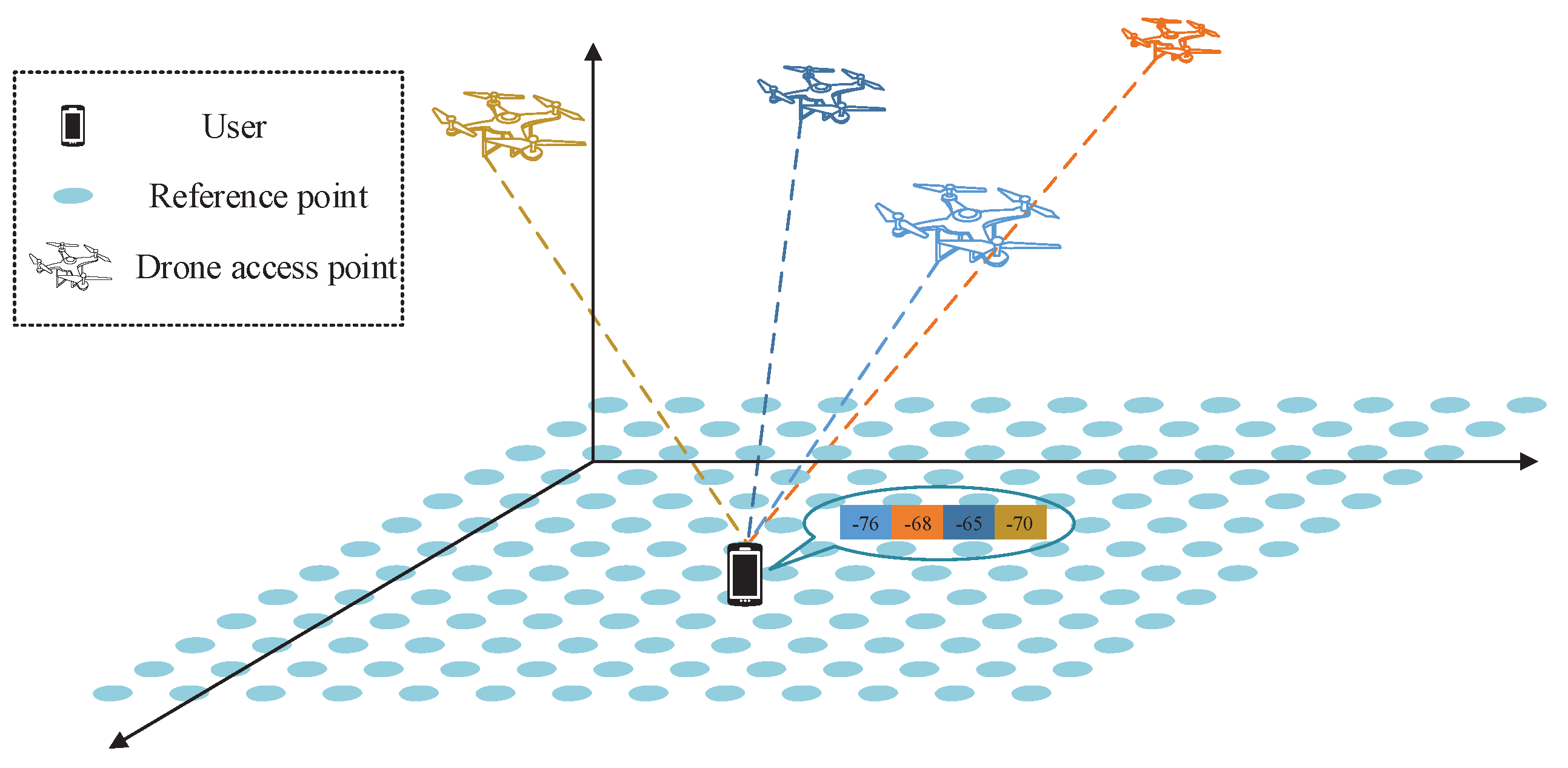
To clearly articulate the system architecture and facilitate subsequent research and analysis, we first establish some basic symbols, and the system framework is shown in Figure 1. Assume there are n drone access points (dAPs) and M reference points (RPs) within this localization area, to construct a complete network coverage range and provide accurate location information. The position coordinates of each RP are recorded as $p_j(x_j,y_j)$, and the information of these M reference points (RPs) forms a position space $\mathit{P}={({\mathit{p}}_1,{\mathit{p}}_2,\cdots ,{\mathit{p}}_M)}^T$. Next, we collected RSSI signals from n dAPs at each RP. To obtain a stable RSSI value, we need to perform q acquisitions for each reference node and then average the RSSI values of these q acquisitions and use them as the original location fingerprint information of this reference node $p_j(x_j,y_j)$. This results in an n-dimensional vector ${\mathit{f}}_{\mathit{j}}={({\mathit{rss}}_j^1,{\mathit{rss}}_j^2,\cdots ,{\mathit{rss}}_j^n)}^T,j\in (1,M)$ of original location fingerprints, where each dimension corresponds to a dAP and contains the mean RSSI value of that dAP at that reference node, where ${\mathit{rss}}_j=\frac{1}{q}{\sum }_{i=1}^q{\mathit{rss}}_{(j,i)}$ in this vector represents the mean RSSI value from the jth dAP after 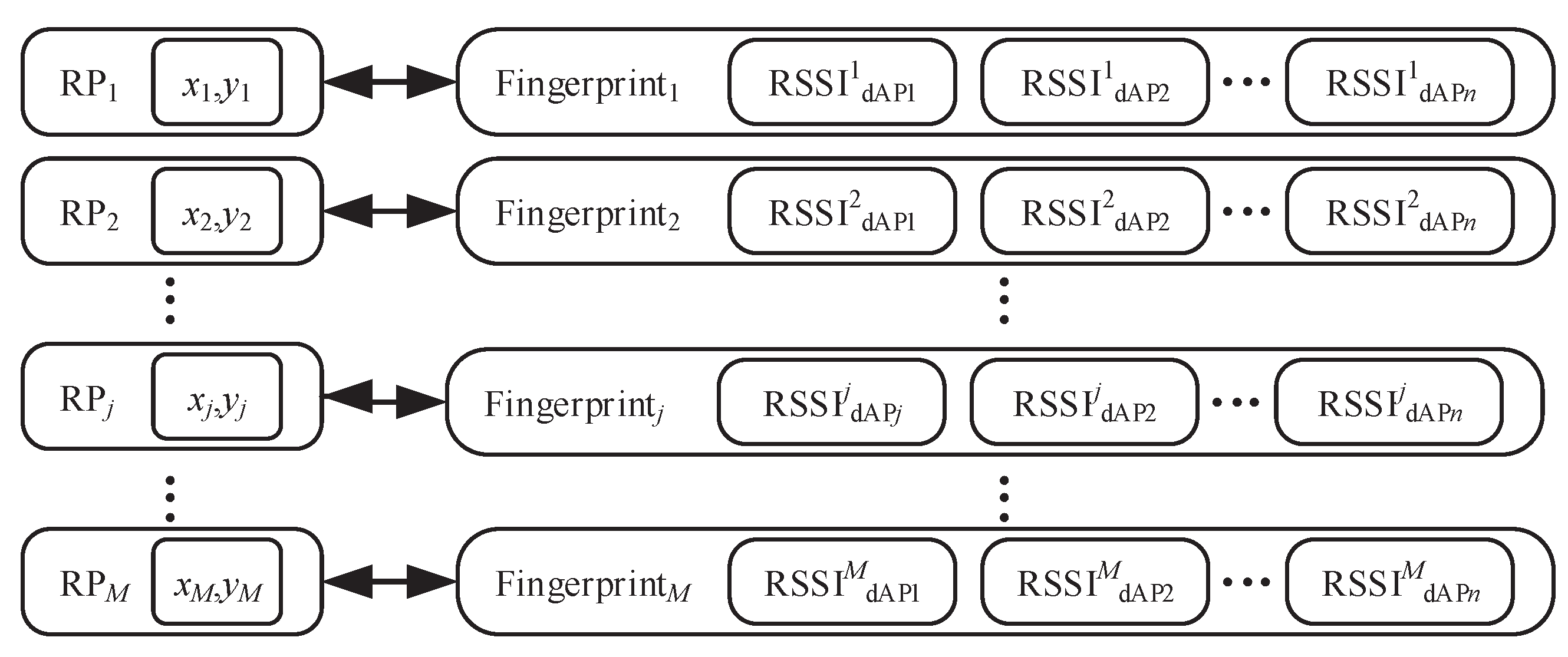q samples. The original location fingerprint information of each reference node is stored in the offline fingerprint database by a data storage technique, forming an original location fingerprint space $\mathit{F}={({\mathit{f}}_1,{\mathit{f}}_2,\cdots ,{\mathit{f}}_M)}^T$ containing $M\times n$ dimensions, as shown in Figure 2.

Each row vector in the matrix $\mathit{F}$ is a vector consisting of multiple features, which reflect the location fingerprints of the reference nodes. The raw location fingerprint data are trained by using the KGLPP method, from which features for localization are extracted. The feature location fingerprint space ${\mathit{F}}^{\prime }={({{\mathit{f}}^{\prime }}_1,{{\mathit{f}}^{\prime }}_2,\cdots ,{{\mathit{f}}^{\prime }}_M)}^T$ consists of the extracted localization features and corresponds to the original location fingerprint space $\mathit{P}$, that is the feature location fingerprint of $p_j(x_j,y_j)$ is ${{\mathit{f}}^{\prime }}_j$. During online positioning, we collected g samples of RSSI signals at the target location to be positioned. By calculating the average value, we used it as the online fingerprint $\mathit{T}=({\mathit{t}}_1,{\mathit{t}}_2,\cdots ,{\mathit{t}}_n)$ for online fingerprinting, as shown in Figure 3. Next, we applied the KGLPP algorithm to $\mathit{T}$ to extract the online feature fingerprint vector ${\mathit{T}}^{\prime }=({{\mathit{t}}^{\prime }}_1,{{\mathit{t}}^{\prime }}_2,\cdots ,{{\mathit{t}}^{\prime }}_n)$. Then, a modified weighted k-nearest neighbor (IWKNN) algorithm was used to estimate the location of the target by comparing ${\mathit{T}}^{\prime }$ with the feature location fingerprint vector in the offline location fingerprint library.

4. KGLPP Positioning Algorithm

4.1. KGLPP Transform of Original Position Fingerprint

Kernel global locally preserving projection (KGLPP) is a new nonlinear dimension-reduction method by introducing a kernel function into GLPP. Use nonlinear mapping $\varphi$ to realize the mapping from the original location fingerprint space $\mathit{F}\in {\mathit{R}}^{n\times M}$ to the feature space, that is ${\mathit{f}}_1,{\mathit{f}}_2,\cdots ,{\mathit{f}}_M$ is transformed into the sample point $\varphi \left({\mathit{f}}_1\right),\varphi \left({\mathit{f}}_2\right),\cdots ,\varphi \left({\mathit{f}}_M\right)$ of the feature space, and assume that the data in the feature space meet the centralization condition, as shown in (20):

$$\sum _{i=1}^M\varphi \left({\mathit{f}}_i\right)=0$$

(20)

It can be seen from Equation (18) that the eigenvector problem of KGLPP is as follows:

$$\varphi \left(\mathit{F}\right)\mathit{L}{\varphi }^T\left(\mathit{F}\right)\mathit{V}=\lambda (\mu \varphi \left(\mathit{F}\right)\mathit{H}{\varphi }^T\left(\mathit{F}\right)+(1-\mu )\mathit{I})\mathit{V}$$

(21)

The feature vector $\mathit{V}$ belongs to the space generated by $\varphi \left({\mathit{f}}_1\right),\varphi \left({\mathit{f}}_2\right),\cdots ,\varphi \left({\mathit{f}}_M\right)$, and all feature vectors can be obtained by linearly combining $\varphi \left({\mathit{f}}_1\right),\varphi \left({\mathit{f}}_2\right),\cdots ,\varphi \left({\mathit{f}}_M\right)$. This combination can be represented using linear tensors, as shown in Equation (22).

$$\mathit{V}=\sum _{i=1}^M{\mathit{\alpha }}_i\varphi \left({\mathit{f}}_i\right)=\mathit{\alpha }\varphi \left(\mathit{F}\right)$$

(22)

where $\mathit{\alpha }={[{\mathit{\alpha }}_1,{\mathit{\alpha }}_2,\cdots ,{\mathit{\alpha }}_M]}^T\in {\mathit{R}}^M$, in Equation (21); multiplying ${\varphi }^T\left(\mathit{F}\right)$ on the left-hand side of the equation, respectively, yields the new equation:

$${\varphi }^T\left(\mathit{F}\right)\varphi \left(\mathit{F}\right)\mathit{L}{\varphi }^T\left(\mathit{F}\right)\mathit{V}=\lambda {\varphi }^T\left(\mathit{F}\right)(\mu \varphi \left(\mathit{F}\right)\mathit{H}{\varphi }^T\left(\mathit{F}\right)+(1-\mu )\mathit{I})\mathit{V}$$

(23)

Substituting Equation (22) into Equation (23), a new expression can be obtained. To represent this new expression more conveniently, a kernel matrix $\mathit{K}\in {\mathit{R}}^{M\times M}$ can be defined:

$${\mathit{K}}_{ij}=\mathit{k}({\mathit{f}}_i,{\mathit{f}}_j)=\varphi \left({\mathit{f}}_i\right)·\varphi \left({\mathit{f}}_j\right)={\varphi }^T\left({\mathit{f}}_i\right)\varphi \left({\mathit{f}}_j\right)$$

(24)

Thus, Equation (23) can be simplified as

$$\tilde{\mathit{K}}\mathit{L}\tilde{\mathit{K}}\mathit{\alpha }=\lambda (\mu \tilde{\mathit{K}}\mathit{H}\tilde{\mathit{K}}+(1-\mu )\tilde{\mathit{K}})\mathit{\alpha }$$

(25)

where $\tilde{\mathit{K}}$ represents the modified kernel matrix. Generally speaking, the data in the feature space do not satisfy the centralization condition, which means that Equation (20) is not valid. Therefore, it is necessary to adjust the data in the feature space to ensure that this condition is met in practical applications. This adjustment process can be expressed using Equation (26).

$$\tilde{\varphi }\left({\mathit{f}}_i\right)=\varphi \left({\mathit{f}}_i\right)-\frac{1}{M}\sum _{j=1}^M\varphi \left({\mathit{f}}_j\right)$$

(26)

To simplify the expression, for M-dimensional vectors, we can introduce an M-dimensional column vector ${\mathit{1}}_{M\times 1}={[\mathit{1},\mathit{1},\cdots ,\mathit{1}]}^T$, where each element is equal to 1. Therefore, Equation (26) can be expressed as:

$$\tilde{\varphi }\left({\mathit{f}}_i\right)=\varphi \left({\mathit{f}}_i\right)-\frac{1}{M}\varphi \left(\mathit{F}\right)1_{M\times 1}$$

(27)

The centering operation is performed on all vectors in matrix $\varphi \left(\mathit{F}\right)$, i.e.,

$$\begin{array}{cc}\hfill \tilde{\varphi }\left(\mathit{F}\right)& =[\varphi \left({\mathit{f}}_1\right),\varphi \left({\mathit{f}}_2\right),\cdots ,\varphi \left({\mathit{f}}_M\right)]-\frac{1}{M}\varphi \left(\mathit{F}\right){\mathit{1}}_{M\times 1}{{\mathit{1}}_{M\times 1}}^T\hfill \\ \hfill & =\varphi \left(\mathit{F}\right)-\frac{1}{M}\varphi \left(\mathit{F}\right){\mathit{1}}_{M\times 1}{{\mathit{1}}_{M\times 1}}^T\hfill \end{array}$$

(28)

For convenient representation and simplification of notation, we used the matrix ${\mathit{1}}_{\mathit{M}}=\frac{1}{M}{\mathit{1}}_{M\times 1}{{\mathit{1}}_{M\times 1}}^T$ to represent an $M\times M$ matrix, which is composed of elements that are all equal to $\frac{1}{M}$. With this in mind, $\tilde{\varphi }\left(\mathit{F}\right)$ can be represented in a more-compact form:

$$\tilde{\varphi }\left(\mathit{F}\right)=\varphi \left(\mathit{F}\right)-\varphi \left(\mathit{F}\right)1_M$$

(29)

Therefore, the modified kernel matrix expression is

$$\begin{array}{cc}\hfill \tilde{\mathit{K}}& =\tilde{\varphi }{\left(\mathit{F}\right)}^T\tilde{\varphi }\left(\mathit{F}\right)\hfill \\ \hfill & ={[\varphi \left(\mathit{F}\right)-\varphi \left(\mathit{F}\right)1_M]}^T[\varphi \left(\mathit{F}\right)-\varphi \left(\mathit{F}\right)1_M]\hfill \\ \hfill & =\mathit{K}-\mathit{K}·{\mathit{1}}_M-{\mathit{1}}_M·\mathit{K}+{\mathit{1}}_M·\mathit{K}·{\mathit{1}}_M\hfill \end{array}$$

(30)

Thus, we can obtain the $\mathit{K}$ value by performing calculations on the raw data $\mathit{F}$ and then calculate the centralized $\tilde{\mathit{K}}$ matrix according to the above formula, assuming the first $l(l\le M$) maximum eigenvalues ${\lambda }_1\ge {\lambda }_2\ge \cdots {\lambda }_{l-1}\ge {\lambda }_l$ from Equation (25), along with their corresponding l unit orthogonal eigenvectors $\mathit{\alpha }={[{\mathit{\alpha }}_1,{\mathit{\alpha }}_2,\cdots ,{\mathit{\alpha }}_l]}^T$. Feature extraction in the feature space $\varphi \left(\mathit{F}\right)$ is performed by calculating the projection of $\varphi \left(\mathit{F}\right)$ onto the eigenvector space. The projection of the ith sample onto the kth coordinate axis ${\mathit{V}}_k$ is given by Equation (31).

$$\begin{array}{cc}\hfill {\mathit{t}}_{ki}& ={\varphi }^T\left({\mathit{f}}_i\right){\mathit{V}}_k\hfill \\ & ={\varphi }^T\left({\mathit{f}}_i\right)\sum _{j=1}^M{\mathit{\alpha }}_{kj}\varphi \left({\mathit{f}}_j\right)\hfill \\ & =\sum _{j=1}^M{\mathit{\alpha }}_{kj}{\varphi }^T\left({\mathit{f}}_i\right)\varphi \left({\mathit{f}}_j\right)\hfill \\ \hfill & =\sum _{j=1}^M{\mathit{\alpha }}_{kj}\tilde{\mathit{K}}({\mathit{f}}_i,{\mathit{f}}_j)\hfill \\ & =\sum _{j=1}^M{\mathit{\alpha }}_{kj}{\tilde{\mathit{K}}}_{ij}\hfill \end{array}$$

(31)

To make it more compact, the entire feature space $\varphi \left(\mathit{F}\right)$ is projected onto ${\mathit{V}}_k$ to obtain Equation (32).

$${\mathit{t}}_k={\varphi }^T\left(\mathit{F}\right)\varphi \left(\mathit{F}\right){\mathit{\alpha }}_k=\tilde{\mathit{K}}{\mathit{\alpha }}_k$$

(32)

Computing using Equation (32) yields the feature position fingerprint space ${\mathit{F}}^{\prime }$, which is composed of $\tilde{\mathit{K}}\mathit{\alpha }$, where $\mathit{\alpha }={({\mathit{\alpha }}_1,{\mathit{\alpha }}_2,\cdots ,{\mathit{\alpha }}_l)}^T$ is an $l\times M$-dimensional matrix. This means that, by using the KGLPP processing method, we can transform the original $n\times M$-dimensional position fingerprint space into a low-dimensional $l\times M(l\le n)$ feature position fingerprint space ${\mathit{F}}^{\prime }$, thereby simplifying the data representation and reducing computational complexity.

In this algorithm, selecting the Gaussian kernel function as the kernel function can effectively handle nonlinear problems. The Gaussian kernel function has a smooth shape, which can smooth the input data, and can be adjusted to different datasets by adjusting the parameters appropriately. Therefore, choosing the Gaussian kernel function in the KGLPP algorithm can improve the accuracy and stability of the model and better handle complex datasets. The Gaussian kernel function can be expressed mathematically as shown in Equation (33).

$$k(x_i,x_j)=exp\left(\frac{\left|\right|x_i-x_j\left|\right|}{-{\gamma }^2}\right)$$

(33)

The flow chart shown in Figure 4 illustrates the process of the KGLPP algorithm.

4.2. Selection of Balance Parameter $\mu$

The selection of balance parameter $\mu$ is very important for KGLPP. It is used to balance the impact of global and local information in node-embedding algorithms. The value range of this parameter is $0\sim 1$. The closer it is to 1, the more emphasis is placed on local information; the closer it is to 0, the more emphasis is placed on global information. Choosing the appropriate balancing coefficient can be adjusted according to the characteristics of the dataset. A larger balance parameter places greater emphasis on the protection of the local structure, while a smaller balance parameter places greater emphasis on the protection of the global structure. In order to achieve a balance between protecting local and global structures, $\mu$ can be chosen according to the following rules.

$$\mu S_{Local}=(1-\mu )S_{Global}$$

(34)

In this formula, $S_{Local}=\rho \left(Q\right)$ and $S_{Global}=\rho \left(\tilde{Q}\right)$ represent the scales of maintaining local and global structures, respectively, where $\rho (·)$ denotes the matrix’s spectral radius. Thus, $\mu$ is

$$\mu =\frac{\rho \left(\tilde{Q}\right)}{\rho \left(Q\right)+\rho \left(\tilde{Q}\right)}$$

(35)

By choosing the lower and upper bounds of $\mu$, two special instances of the KGLPP algorithm can be obtained. When $\mu =0$ and the non-weighted adjacency matrix $\tilde{\mathit{W}}=1_{n\times n}$, this means the neighborhood relationships between the data points are ignored. In this case, Equation (25) will become more-simplified:

$$-\tilde{\mathit{K}}\tilde{\mathit{Q}}\tilde{\mathit{K}}\mathit{\alpha }=\lambda \tilde{\mathit{K}}\mathit{\alpha }$$

(36)

where $\tilde{\mathit{Q}}=\tilde{\mathit{D}}-\tilde{\mathit{W}}\in {\mathit{R}}^{n\times n}$ is a symmetric matrix and, in particular, for undirected graphs, $\tilde{\mathit{W}}$ is also symmetric. The diagonal elements of $\tilde{\mathit{Q}}$ are ${\tilde{\mathit{q}}}_{ii}=n-1$, and the off-diagonal elements are ${\tilde{\mathit{q}}}_{ij}=-1(i\ne j)$. It can be intuitively observed that, if the sample size n is large enough and the matrix $\frac{\tilde{\mathit{Q}}}{n}$ is approximately equal to the identity matrix, an approximate solution to Equation (37) can be obtained.

$$\tilde{\mathit{K}}\tilde{\mathit{K}}\mathit{\alpha }=-\frac{\lambda }{n}\tilde{\mathit{K}}\mathit{\alpha }\to \tilde{\mathit{K}}\mathit{\alpha }=\tilde{\lambda }\mathit{\alpha }$$

(37)

This is equivalent to the eigenvector problem in Equation (7) of KPCA, except that their eigenvalues are scaled according to different coefficients. Therefore, KPCA can be regarded as a special case of the KGLPP problem; it only considers the global data structure. On the other hand, if we choose $\mu =1$ and ignore the contribution of the global data structure, Equation (25) will be simplified to

$$\tilde{\mathit{K}}\mathit{Q}\tilde{\mathit{K}}\mathit{\alpha }=\lambda \tilde{\mathit{K}}\mathit{D}\tilde{\mathit{K}}\mathit{\alpha }$$

(38)

This is exactly the process of solving the eigenvector problem in KLPP represented by Equation (11). Therefore, KLPP can be regarded as another special case of KGLPP that only preserves local structure information without considering global structure information.

4.3. Online Location Fingerprint Processing

During online positioning, we collected g RSSI signal samples as $\mathit{R}={({\mathit{r}}_1,{\mathit{r}}_2,\cdots ,{\mathit{r}}_g)}^T$ at the target location to be located. Then, calculate the mean of each column of R. We used it as the online fingerprint $\mathit{T}=({\mathit{t}}_1,{\mathit{t}}_2,\cdots ,{\mathit{t}}_n)$ for online fingerprinting. To ensure consistency between offline and online data, we need to perform KGLPP training on the online RSSI vectors before target positioning. Apart from the different expressions of the correlation variables, the online KGLPP training process is consistent with the offline process. By processing the online RSSI signal using KGLPP, the vector–matrix ${\mathit{T}}^{\prime }=({{\mathit{t}}^{\prime }}_1,{{\mathit{t}}^{\prime }}_2,\cdots ,{{\mathit{t}}^{\prime }}_n)$ is obtained. ${\mathit{T}}^{\prime }$ can now be used for target positioning.

$$\mathit{T}=\frac{{\sum }_{i=1}^{g}r}{g}=({\mathit{t}}_1,{\mathit{t}}_2,\cdots ,{\mathit{t}}_n)$$

(39)

4.4. IWKNN Positioning

Calculate the Euclidean distance between the online location fingerprint ${\mathit{T}}^{\prime }$ and each fingerprint ${\mathit{F}}^{\prime }$ in the offline fingerprint database, as shown in the following equation.

$${\mathit{D}}_j({\mathit{T}}^{\prime },{{\mathit{F}}^{\prime }}_j)=\sqrt{\sum _{i=1}^l{({{\mathit{t}}^{\prime }}_i-{{\mathit{rss}}^{\prime }}_{ji})}^2},j\in (1,M)$$

(40)

${\mathit{D}}_j({\mathit{T}}^{\prime },{{\mathit{F}}^{\prime }}_j)$ is a measure of the similarity between ${\mathit{T}}^{\prime }$ and ${{\mathit{F}}^{\prime }}_j$. The smaller its value, the more similar $\mathit{T}$ and ${{\mathit{F}}^{\prime }}_j$ are to each other. ${{\mathit{F}}^{\prime }}_j$ is a vector representation of specific features extracted at location $p_j(x_j,y_j)$, which can be used to describe the feature information at that location. Arrange these similarities ${\mathit{D}}_j$ in order from smallest to largest, and find the h feature location fingerprints and location information $p_j(x_j,y_j)$ corresponding to the top h smallest similarity values, such that

$$\frac{{\sum }_{j=1}^h\frac{1}{{\mathit{D}}_j+l_0}}{{\sum }_{j=1}^M\frac{1}{{\mathit{D}}_j+l_0}}\ge \sigma$$

(41)

where $l_0$ is set to a very small number to avoid the denominator being zero. $\sigma$ is a positive number less than 1, which measures the importance of the location fingerprint in terms of the cumulative contribution. Specifically, when a location fingerprint is added to the cumulative contribution, the degree of its impact on the total contribution is limited by $\sigma$, i.e., the smaller $\sigma$ is, the smaller the impact of that location fingerprint on the total contribution. The purpose of this design is to balance the contribution of each location fingerprint and prevent certain location fingerprints from being too prominent in their contribution and affecting the performance of the whole system.

Equation (41) provides a method to determine the magnitude of the h value autonomously, i.e., by calculating the value of h given the number of position fingerprints M and $\sigma$. After determining the value of h, we can use Equation (42) to calculate the location estimate $(\widehat{x},\widehat{y})$.

$$(\widehat{x},\widehat{y})=\frac{{\sum }_{j=1}^h\left(\frac{1}{{\mathit{D}}_j+l_0}{p}_j\right)}{{\sum }_{j=1}^h\frac{1}{{\mathit{D}}_j+l_0}}$$

(42)

4.5. Complexity Analysis of KGLPP

We conducted the following analysis on the complexity of KGLPP. The dimension of the fingerprint dataset is [M, n], where M represents the number of samples and n represents the sample dimension:

(1)

For a given dataset, we need to calculate the Euclidean distance between each pair of samples. The complexity of this calculation is $O\left(M^{2}n\right)$.

(2)

The complexity of computing the output value of the Gaussian kernel is $O\left(M^2\right)$.

(3)

The complexity of constructing an adjacency weight matrix is $O\left(M^{2}log\left(M\right)\right)$.

(4)

The complexity of constructing a non-adjacency weight matrix is $O\left(M^{2}log\left(M\right)\right)$.

(5)

The complexity of constructing the objective function is $O\left(M^2\right)$.

(6)

The complexity of eigenvalue decomposition is $O\left(n^3\right)$.

(7)

The overall complexity of KGLPP is mainly determined by the distance calculation and eigenvalue decomposition, which is $O(M^{2}n+n^3)$.

5. Simulation and Experiment

In this paper, we used simulation data to verify the effectiveness of our proposed algorithm. We selected the following four existing algorithms for comparison, which have been widely used for similar problems:

(1)

KNN [33]: During online localization, the Euclidean distance is used to find the RPs closest to the target, and the average position of these RPs is used to estimate the position of the target.

(2)

WKNN [34]: WKNN differs from KNN in that it assigns different weights to different RPs when estimating the target location.

(3)

KPCA-IWKNN [25]: The KPCA-IWKNN algorithm combines the KPCA and IWKNN algorithms, using the KPCA algorithm to downscale and extract features from the data, then using the IWKNN algorithm to localize the target.

(4)

KLPP-IWKNN [31]: The KLPP-IWKNN algorithm uses the KLPP algorithm for feature extraction and dimensionality reduction first and then uses the improved IWKNN algorithm for localization.

In this experiment, we evaluated and compared five different methods using three metrics: mean error (ME), localization accuracy, and cumulative distribution function (CDF). The mean error is the average distance between the estimated position of the positioning system and the real position. Assuming that the real position of target j is $Z_j$ and its estimated position is $Z_j^{\prime }$ according to the prediction of the localization system, the localization error is $E_j=\left|\right|Z_j^{\prime }-Z_j\left|\right|$, and the ME is obtained according to N times of localization as

$$ME=\frac{1}{N}\sum _{j=1}^N{E}_j.$$

(43)

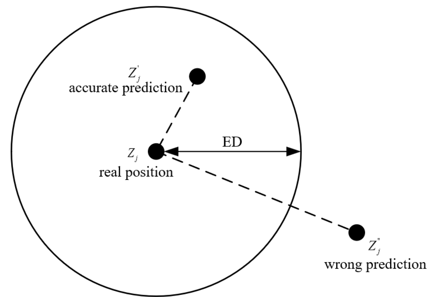
Localization accuracy is an important metric for assessing the performance of a localization system and measures the degree of agreement between the localization results and the true position [25]. Localization errors are known to be an unavoidable problem in localization systems because they are influenced by a variety of factors. Therefore, in practical applications, the localization error is acceptable for a certain range, but if the localization error exceeds this range, then it may lead to the degradation of system performance and unsatisfactory application results. Suppose the actual position of the target to be measured is $Z_j$ for a given allowable error distance (ED) and the position of the target is predicted by the localization system to obtain the predicted position as $Z_j^{\prime }$. If the distance between the predicted position $Z_j^{\prime }$ and the real position $Z_j$ is less than ED, we can assume that this localization is accurate. That is, if $|Z_j^{\prime }-Z_j|\le ED$, then $Z_j^{\prime }$ is accurate localization; conversely, if $|Z_j^{″}-Z_j|>ED$, then $Z_j^{″}$ is the wrong localization. The concept of accurate localization is illustrated in Figure 5. Specifically, localization accuracy is the ratio of the number of accurate positions to the total number of positions when the localization system performs multiple localization tasks. Assuming the total number of localization is B, the number of accurate localization is C, and the accuracy of localization is E, the expression for the accuracy of localization is:

$$E=\frac{C}{B}$$

(44)

5.1. Simulation Settings

In this paper, we verified the algorithm using simulation data to evaluate the performance of the algorithm. In this simulation experiment, we used a specific simulation environment with the following relevant parameters. We used an Asus laptop (Asus, Taipei, Taiwan) as the hardware device and implemented the algorithm on the Matlab 2016a software platform.

To better simulate real-world scenarios, a two-ray ground reflection (TRGR) channel path loss model was adopted to construct the fingerprint database [35]. Specifically, the path loss of the TRGR channel is expressed as follows:

$$PL=10{log}_{10}\left(\frac{P_t}{P_r}\right)+x=10{log}_{10}\left({\left|\frac{\lambda }{4\pi }\left(\frac{\sqrt{G_{los}}}{s}+\frac{\Gamma \left(\theta \right)\sqrt{G_{gr}}{e}^{-j\Delta \phi }}{s^{\prime }}\right)\right|}^2\right)+x,x\sim N(0,{\delta }^2)$$

(45)

where s represents the length of the line-of-sight (LOS) path, $s^{\prime }$ represents the length of the ground reflection path, while d represents the horizontal distance between the transmitter and receiver. $h_t$ represents the height of the transmitter, and $h_r$ represents the height of the receiver. $G_{los}$ represents the combined antenna gain along the LOS path; $G_{gr}$ represents the combined antenna gain along the ground reflection path; $\lambda$ denotes the wavelength of transmission; $\Gamma \left(\theta \right)$ represents the reflection coefficient, where $\theta =actan\left(\frac{h_t+h_r}{d}\right)$ and $x\sim N(0,{\delta }^2)$ is the noise.

To simulate a realistic wireless communication environment, the parameters for the TRGR model path loss were set as follows: the length of $h_t$ was 2.5 m; the length of $h_r$ was 1.55 m; $\lambda$ was 0.123 m (where the carrier frequency was 2440 MHz); $\Gamma \left(\theta \right)=\frac{sin\left(\theta \right)-x_v}{sin\left(\theta \right)+x_v}$, where $x_v=\frac{\sqrt{ϵ-cos{\left(\theta \right)}^2}}{ϵ}$, $ϵ=4.5+0.5i$ was used to represent the relative permittivity of dry soil.

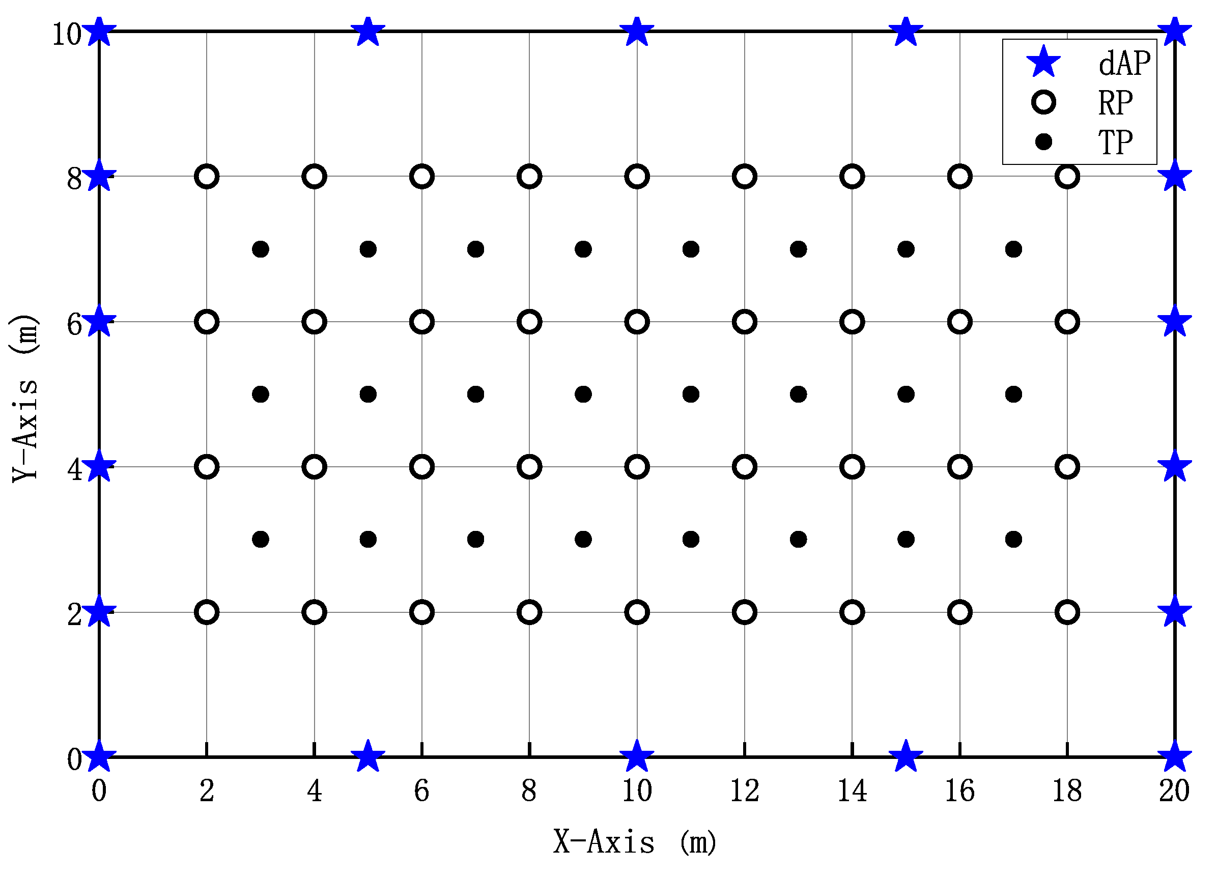
In order to verify the effectiveness of the algorithm, we needed to establish a reliable test environment first. We chose a basic fingerprint location method and set up a topographic map as a base before testing. As shown in Figure 6. The topographic map was 20 m $\times 10$ m; the size of the RP grid was 2 m; the number of dAPs was 18. To ensure accuracy, the RSSI data of each RP and TP were collected 100 times. By averaging the collected data, more reliable and stable mean values can be obtained, enabling a more-accurate assessment of the signal strength between the RPs and TPs.

During the simulation process, we employed the Gaussian kernel function as the kernel function for KGLPP, KPCA, and KLPP. The width $\gamma$ of the Gaussian kernel function was empirically set to 2. For the WKNN and KNN algorithms, we chose the four nearest neighbors to compute the similarity. The value of $\sigma$ was set to be 0.3.

5.2. Illustrative Results

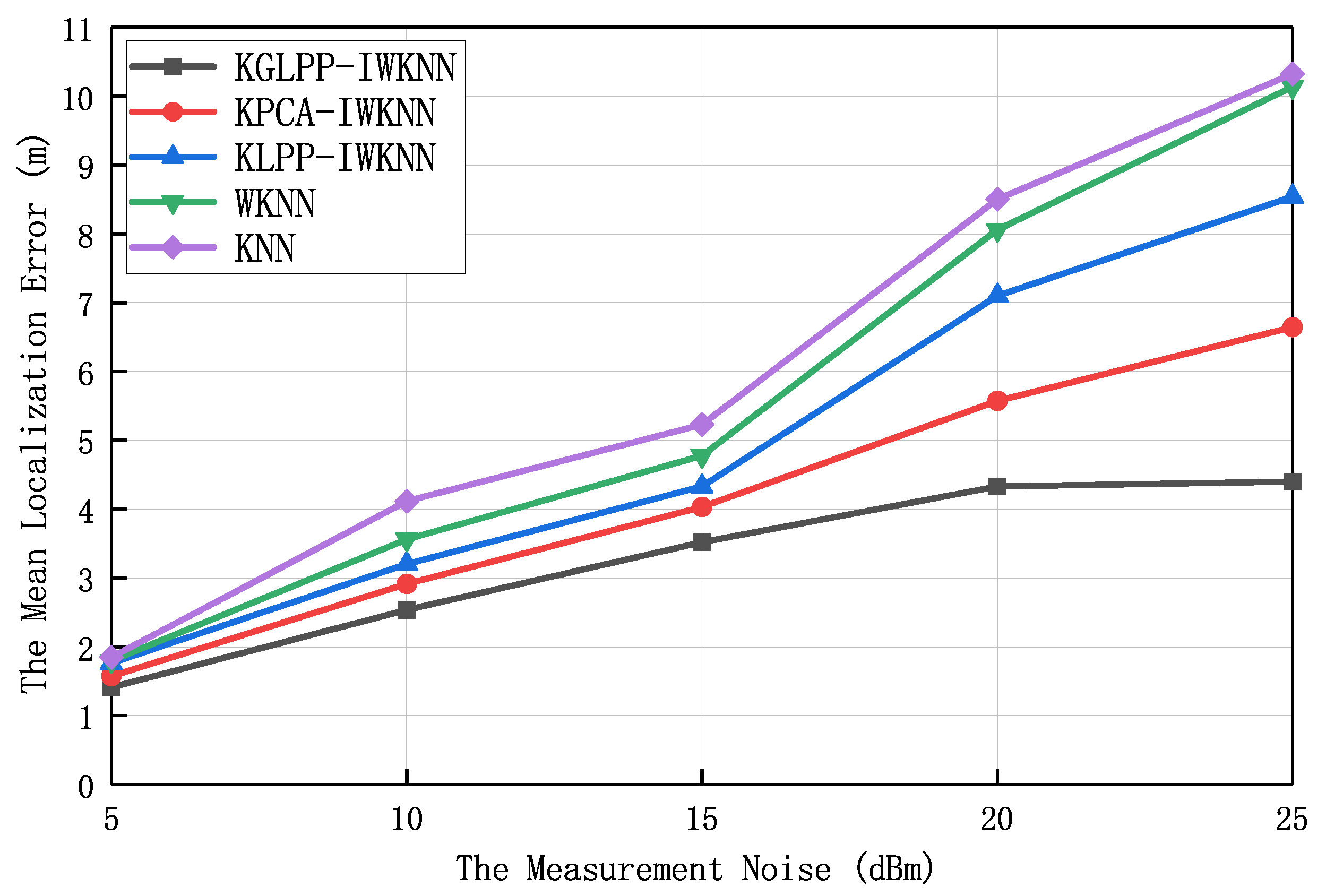
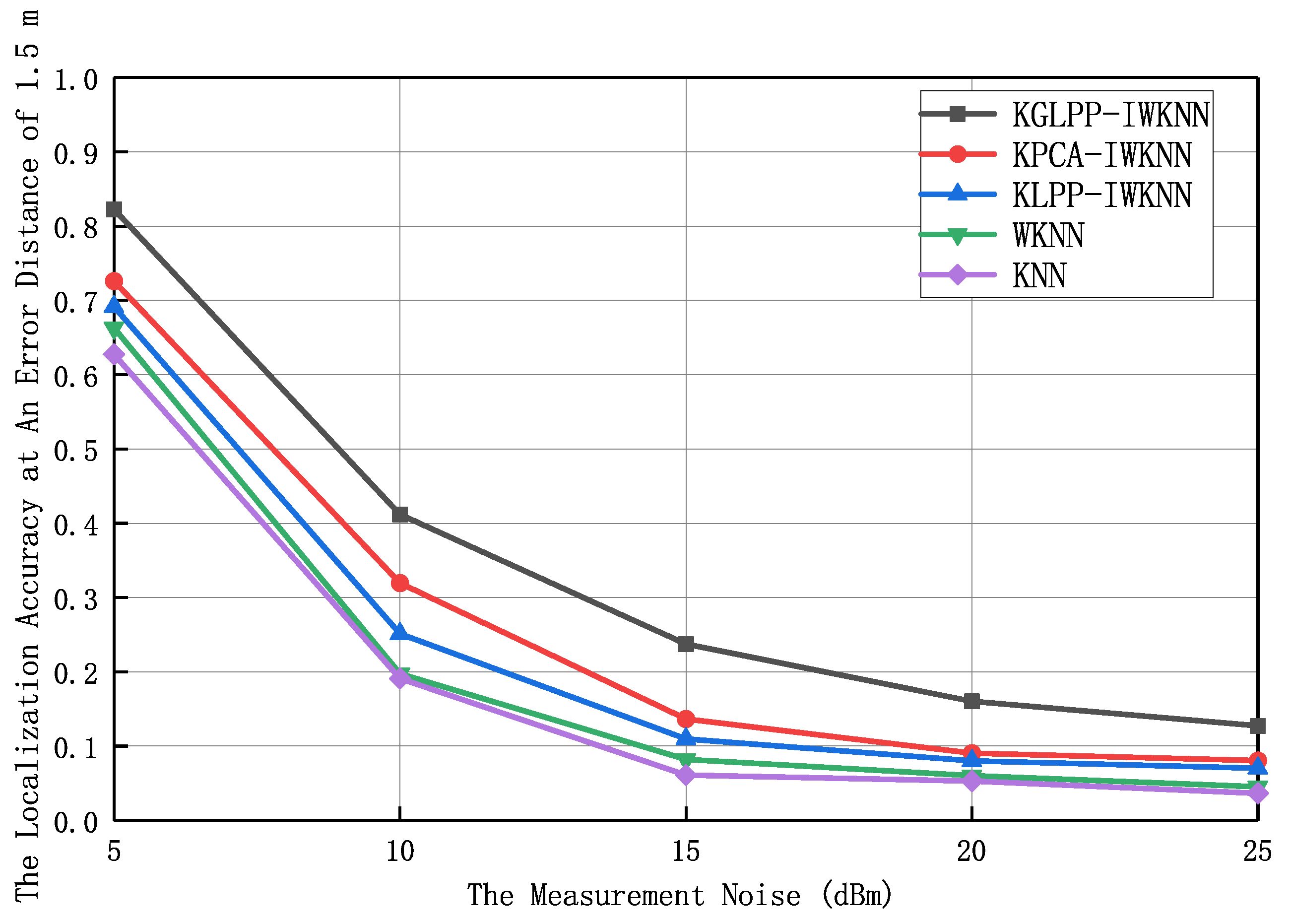
Figure 7 and Figure 8 illustrate the trend of algorithmic localization accuracy variation when the random noise intensity (The random noise intensity refers to the degree or strength of the random noise introduced into the fingerprint data during the simulation process. It is a parameter in the simulation environment used to control the intensity and range of the noise impact.) was within the range of 5 dBm to 25 dBm, with an average localization error and error distance of 1.5 m. In this experiment, the number of dAPs was 18, the value of $\sigma$ was 0.3, and the dimension of the feature location fingerprint space was eight. The results in the figures show that the localization performance and localization accuracy of all localization algorithms gradually decreased when the noise increased. The algorithm proposed in this paper outperformed the other four algorithms in terms of average positioning error and positioning accuracy. This advantage stemmed from the ability of KGLPP to maintain both global and local structural information during the dimensionality reduction process. It takes into account not only the similarity between data samples (local structure), but also the characteristics of the overall data distribution (global structure). By constructing a graphical structure in high-dimensional space and using the graph Laplacian operator for dimensionality reduction, KGLPP is able to preserve the relationships between data samples, thereby maintaining the structure and geometric properties of the data as much as possible after dimensionality reduction. When there is noise present, KPCA and KLPP often suffer from interference, leading to distorted results after dimensionality reduction. In contrast, KGLPP effectively mitigates the negative impact of noise by preserving structural information. This is because KGLPP takes into account the similarity between samples when constructing the graphical structure, mapping similar samples to neighboring positions in the reduced-dimensionality space. This similarity constraint helps suppress the influence of noise on the dimensionality-reduction results, thereby improving the accuracy and reliability of the data after dimensionality reduction. With the increase of noise, KGLPP-IWKNN exhibited better performance compared to KPCA-IWKNN and KLPP-IWKNN. This is because KGLPP can better preserve structural information, while KPCA and KLPP perform dimensionality reduction without considering global and local structures, making them susceptible to noise interference. Additionally, KGLPP possesses the characteristics of nonlinear mapping, which enables it to better adapt to the distribution of complex data and further enhance robustness against noise. Therefore, KGLPP-IWKNN can provide more-accurate localization results in the presence of noise.

In the following localization simulation experiments, the random noise in the simulation environment was 20 dBm.

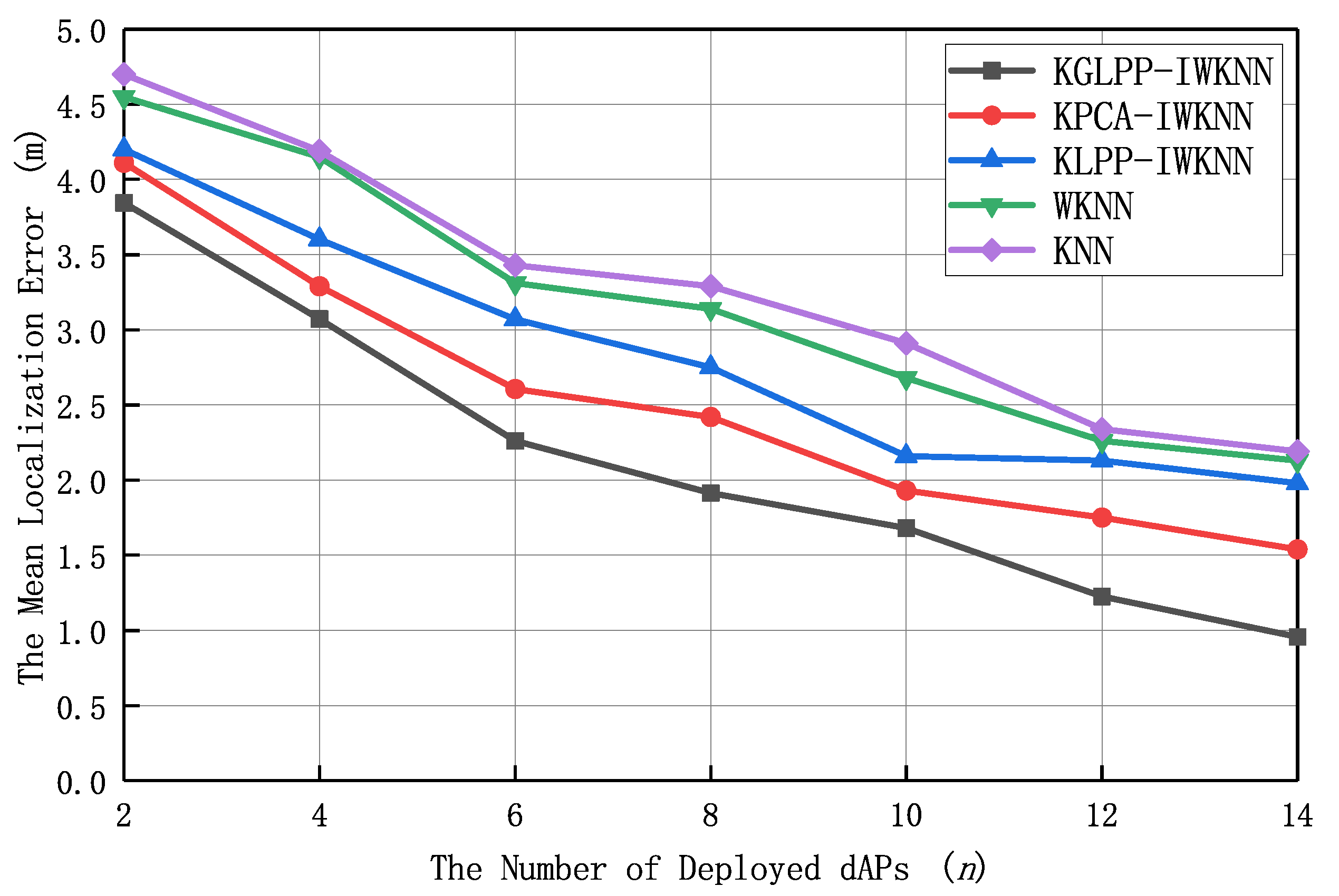
With 100 localization experiments performed, Figure 9 presents the curve of the mean localization error with the number of dAPs when the number of offline deployed dAPs was in the range of 2 to 14. In this experiment, the number of dAPs was 14, the value of $\sigma$ was 0.3, and the dimension of the feature location fingerprint space was eight. As the number of dAPs deployed offline gradually increased, the localization error of all algorithms gradually decreased. This is because the increased number of dAPs led to more matching dimensions, which improved the accuracy of RP matching. In addition, according to the results in Figure 9, when the number of dAPs in the localization area was small, KGLPP-IWKNN exhibited higher localization accuracy compared to other algorithms. This is because KGLPP employs a global–local structure-preservation method during the dimensionality-reduction process, aiming to preserve the spatial layout features of fingerprint data and the relationships between neighboring samples to the greatest extent possible. This global–local structure preservation helps reduce information loss during the dimensionality-reduction process and improves localization accuracy. Moreover, KGLPP also exhibits strong adaptability by dynamically adjusting the projection method during the dimensionality-reduction process based on different signal features. As the number of dAPs increased, the signal features in indoor environments became more diverse and complex. However, KGLPP was able to adapt better to this situation, thereby improving the accuracy of localization. In addition, KGLPP obtained more-representative and -discriminative fingerprint features through feature extraction during the dimensionality reduction process. Compared to methods such as KPCA and KLPP, KGLPP is able to better preserve useful information, effectively differentiate different fingerprint samples when projecting data into a lower-dimensional space, and reduce localization errors.

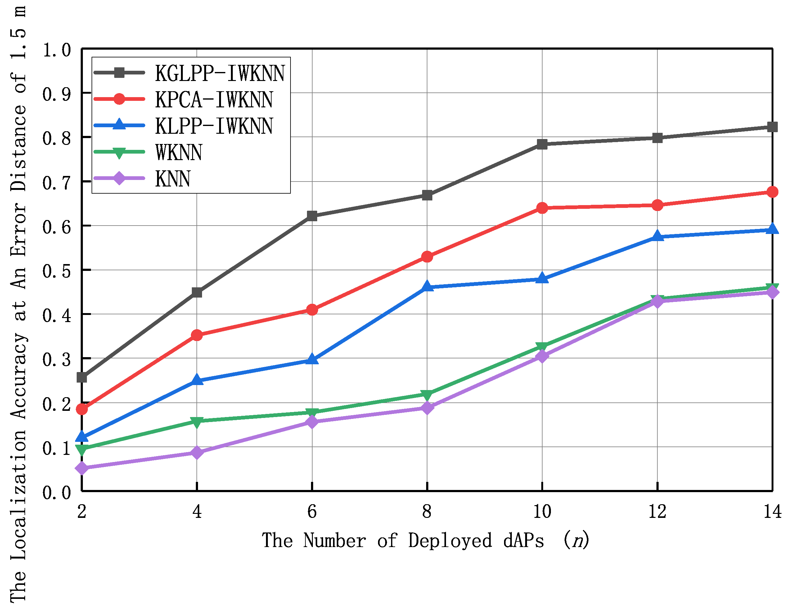
With an error distance of 1.5 m, Figure 10 shows the trend of improved localization accuracy of all algorithms with an increase in the number of dAPs, indicating that the proposed algorithm in this paper had higher localization accuracy compared to the other algorithms. In this experiment, the number of dAPs was 14, the value of $\sigma$ was 0.3, and the dimension of the feature location fingerprint space was eight. When the number of dAPs was six, the proposed algorithm in this paper achieved a localization accuracy of 62%, while other comparative algorithms required more dAPs to achieve this accuracy. This indicated that the algorithm proposed in this paper had higher efficiency in terms of dAP utilization and could achieve higher localization accuracy with a limited number of dAPs.

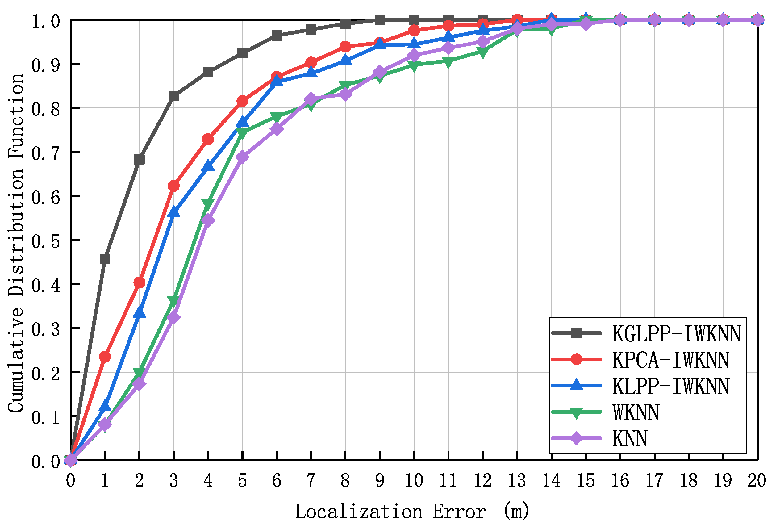
Figure 11 illustrates the cumulative distribution function curve of the localization error. In this experiment, the number of dAPs was 14, the value of $\sigma$ was 0.3, and the dimension of the feature location fingerprint space was eight. Compared with the other algorithms, KGLPP can effectively reduce the data noise and redundancy, preserve useful features, and improve the robustness and discriminability of features. These advantages enable KGLPP to more accurately identify the relationship between the signal strength and location during the localization process, thereby improving the accuracy of localization.

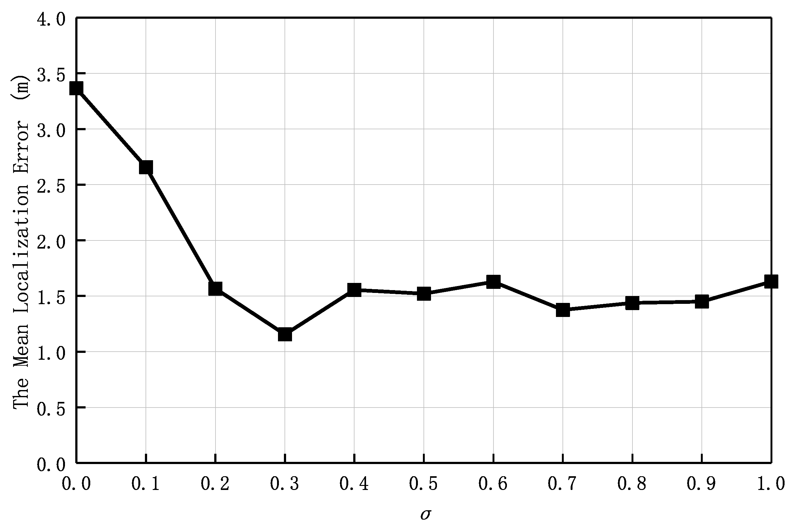
Figure 12 shows the variation of the average localization error of the proposed algorithm with respect to the change of the $\sigma$ value. When $\sigma =0$, the nearest neighbor was used for localization, and the localization error was the highest because only one RP was used for localization, making it very difficult to achieve high-precision localization. As $\sigma$ increased, the number of neighbors required for localization by the IWKNN algorithm also increased, which could more accurately reflect the contribution of RPs and reduce localization error. Therefore, as the $\sigma$ value increased, the average localization error correspondingly decreased. It was found in the experiment that the average localization error reached the minimum value when $\sigma$ was set to 0.3; However, when $\sigma$ was greater than 0.8, in order to improve the accuracy, the algorithm used more neighboring nodes for localization, but these redundant location fingerprints would bring more errors, resulting in an increase in the mean localization error. Therefore, the value of $\sigma$ was set to 0.3 in the experiment to reduce localization errors.

6. Conclusions

This paper aimed to address the issues of limited and non-dynamically adjustable fixed access points (APs) in fingerprint localization and proposed the use of drones as a replacement for traditional APs to improve flexibility and accuracy. Drones can hover at different positions to adapt to various scenarios and user needs. However, factors such as environmental complexity, the massive collection of raw data, and changes in signal strength can all affect the accuracy of fingerprint localization. To address these issues, this study proposed a kernel global locally preserving projection (KGLPP) algorithm that deals with location fingerprint data by reducing dimensionality while taking into account both global and local information, avoiding poor dimensionality reduction due to considering single pieces of information. In the location estimation stage, this paper used an improved weighted k-nearest neighbor (IWKNN) algorithm to more accurately estimate the target location. The IWKNN algorithm is different from the traditional KNN or WKNN algorithms in that it can adaptively select the optimal number of neighbors to improve localization accuracy. The experimental results demonstrated that the algorithm proposed in this paper outperformed other algorithms and achieved higher localization accuracy.

References

1. Lu, C.H.; Chen, P. Robust channel estimation scheme for multi-UAV mmWave MIMO communication with jittering. Electronics 2023, 12, 2102. [Google Scholar] [CrossRef]
2. Zhao, J.W.; Gao, F.F.; Jia, W.M.; Yuan, W.M.; Jin, W. Integrated sensing and communications for UAV communications with jittering effect. IEEE Wirel. Commun. Lett. 2023, 12, 758–762. [Google Scholar] [CrossRef]
3. Cui, Y.P.; Feng, Z.Y.; Zhang, Q.X.; Wei, Z.Q.; Xu, C.L.; Zhang, P. Toward trusted and swift UAV communication: ISAC-enabled dual identity mapping. IEEE Wirel. Commun. 2023, 30, 58–66. [Google Scholar] [CrossRef]
4. Sekander, S.; Tabassum, H.; Hossain, E. Multi-Tier drone architecture for 5G/B5G cellular networks: Challenges, trends, and prospects. IEEE Commun. Mag. 2018, 56, 96–103. [Google Scholar] [CrossRef] [Green Version]
5. Koumaras, H.; Makropoulos, G.; Batistatos, M.; Kolometsos, S.; Kourtis, M.A. 5G-enabled uavs with command and control software component at the edge for supporting energy efficient opportunistic networks. Energies 2021, 14, 1480. [Google Scholar] [CrossRef]
6. Mozaffari, M.; Saad, W.; Bennis, M.; Nam, Y.H.; Debbah, M. A tutorial on UAVs for wireless networks: Applications, challenges, and open problems. IEEE Commun. Surv. Tutor. 2019, 21, 2334–2360. [Google Scholar] [CrossRef] [Green Version]
7. Hyun, J.; Oh, T.; Lim, H.; Myung, H. UWB-based indoor localization using ray-tracing algorithm. In Proceedings of the 2019 16th International Conference on Ubiquitous Robots (UR), Jeju, Republic of Korea, 24–27 June 2019; pp. 98–101. [Google Scholar]
8. Stojkoska, B.R.; Palikrushev, J.; Trivodaliev, K.; Kalajdziski, S. Indoor localization of unmanned aerial vehicles based on RSSI. In Proceedings of the IEEE Eurocon 2017—17th International Conference on Smart Technologies, Ohrid, Macedonia, 6–8 July 2017; pp. 120–125. [Google Scholar] [CrossRef]
9. Wang, T.T.; Cai, Z.H.; Wang, Y.X. UAV indoor vision/inertial navigation integrated navigation method. J. Beijing Univ. Aeronaut. Astronaut. 2018, 44, 176–186. [Google Scholar]
10. Ramirez-Mendoza, R.A. Design and implementation of an iot-oriented strain smart sensor with exploratory capabilities on energy harvesting and magnetorheological elastomer transducers. Appl. Sci. 2020, 10, 4387. [Google Scholar] [CrossRef]
11. Rostami, A.S.; Mohanna, F.; Keshavarz, H. Presenting an optimal energy-aware locating structure using the internet of things and device-to-device communications on smartphones. Wirel. Pers. Commun. 2021, 118, 1745–1774. [Google Scholar] [CrossRef]
12. Li, Y.F.; Ma, S.D.; Yang, G.H.; Wong, K.K. Secure localization and velocity estimation in mobile iot networks with malicious attacks. IEEE Internet Things J. 2020, 8, 6878–6892. [Google Scholar] [CrossRef]
13. Li, Y.F.; Ma, S.D.; Yang, G.H.; Wong, K.K. Robust localization for mixed los/nlos environments with anchor uncertainties. IEEE Trans. Commun. 2020, 68, 4507–4521. [Google Scholar] [CrossRef]
14. Huang, B.; Xu, Z.; Jia, B.; Mao, G. An online radio map update scheme for wifi fingerprint-based localization. IEEE Internet Things J. 2019, 6, 6909–6918. [Google Scholar] [CrossRef]
15. Lorenc, A.; Szarata, J.; Czuba, M. Real-time location system (RTLS) based on the bluetooth technology for internal logistics. Sustainability 2023, 15, 4976. [Google Scholar] [CrossRef]
16. Ma, Y.; Tian, C.; Jiang, Y. A multitag cooperative localization algorithm based on weighted multidimensional scaling for passive UHF RFID. IEEE Internet Things J. 2019, 6, 6548–6555. [Google Scholar] [CrossRef]
17. Cretu-Sircu, A.L. Evaluation and comparison of ultrasonic and UWB technology for indoor localization in an industrial environment. Sensors 2022, 22, 2927. [Google Scholar] [CrossRef]
18. Yang, M.; Wu, H.; Liu, Z.; Ding, S.; Peng, H. Indoor positioning using public fm and dtmb signals based on compressive sensing. China Commun. 2019, 16, 171–180. [Google Scholar] [CrossRef]
19. Xue, J.Q.; Zhang, J.; Gao, Z.Y.; Xiao, W.D. Enhanced WiFi CSI fingerprints for device-free localization with deep learning representations. IEEE Sens. J. 2023, 23, 2750–2759. [Google Scholar] [CrossRef]
20. Zhang, L.; Bao, J.; Xu, Y.; Wang, Q.; Xu, J.; Li, D. From coarse to fine: Two-stage indoor localization with multisensor fusion. Tsinghua Sci. Technol. 2023, 28, 552–565. [Google Scholar] [CrossRef]
21. Dong, Y.H.; He, G.X.; Arslan, T.; Yang, Y.J.; Ma, Y.D. Crowdsourced indoor positioning with scalable WiFi augmentation. Sensors 2023, 23, 4095. [Google Scholar] [CrossRef]
22. Hu, J.S.; Hu, C.W. A WiFi indoor location tracking algorithm based on improved weighted k nearest neighbors and kalman filter. IEEE Access 2023, 11, 32907–32918. [Google Scholar] [CrossRef]
23. Deng, S.H.; Zhang, W.J.; Xu, L.; Yang, J.M. RRIFLoc: Radio robust image fingerprint indoor localization algorithm based on deep residual networks. IEEE Sens. J. 2023, 23, 3233–3242. [Google Scholar] [CrossRef]
24. Kumar, R.; Singh, S.; Chaurasiya, V.K. A low-cost and efficient spatial-temporal model for indoor localization “H-LSTMF”. IEEE Sens. J. 2023, 23, 6117–6128. [Google Scholar] [CrossRef]
25. Li, H.L.; Qian, Z.H.; Tian, H. Research on indoor localization algorithm based on kernel principal component analysis. J. Commun. 2017, 38, 158–167. [Google Scholar] [CrossRef]
26. Schölkopf, B.; Smola, A.; Müller, K.R. Nonlinear component analysis as a kernel eigenvalue problem. Neural Comput. 1998, 10, 1299–1319. [Google Scholar] [CrossRef] [Green Version]
27. He, X.; Niyogi, P. Locality preserving projections. Adv. Neural Inf. Process. Syst. 2003, 10, 16. [Google Scholar] [CrossRef]
28. Luo, L.; Bao, S.; Gao, Z.; Yuan, J. Batch process monitoring with tensor global–local structure analysis. Ind. Eng. Chem. Res. 2013, 52, 18031–18042. [Google Scholar] [CrossRef]
29. Luo, L.; Bao, S.; Gao, Z.; Yuan, J. Tensor global-local preserving projections for batch process monitoring. Ind. Eng. Chem. Res. 2014, 53, 10166–10176. [Google Scholar] [CrossRef]
30. Zhang, M.; Ge, Z.; Song, Z.; Fu, R. Global–local structure analysis model and its application for fault detection and identification. Ind. Eng. Chem. Res. 2011, 50, 6837–6848. [Google Scholar] [CrossRef]
31. Luo, L. Process monitoring with global–local preserving projections. Ind. Eng. Chem. Res. 2014, 53, 7696–7705. [Google Scholar] [CrossRef]
32. Luo, L.; Bao, S.; Mao, J.; Tang, D. Nonlinear process monitoring based on kernel global–local preserving projections. J. Process Control 2016, 38, 11–21. [Google Scholar] [CrossRef]
33. Zhang, H.; Liu, K.; Jin, F.; Feng, L.; Lee, V.; Ng, J. A scalable indoor localization algorithm based on distance fitting and fingerprint mapping in wi-fi environments. Neural Comput. Appl. 2019, 9, 5131–5145. [Google Scholar] [CrossRef]
34. Hou, C.J.; Xie, Y.Q.; Zhang, Z.Z. An improved convolutional neural network based indoor localization by using Jenks natural breaks algorithm. China Commun. 2022, 19, 291–301. [Google Scholar] [CrossRef]
35. Chiu, C.C.; Tsai, A.H.; Lin, H.P.; Lee, C.Y.; Wang, L.C. Channel modeling of air-to-ground signal measurement with two-ray ground-reflection model for UAV communication systems. In Proceedings of the 2021 30th Wireless and Optical Communications Conference (WOCC), Taipei, Taiwan, 7–8 October 2021. [Google Scholar] [CrossRef]
Figure 1. System framework.
Drones 07 00480 g001
Figure 2. Offline fingerprint database.
Drones 07 00480 g002
Figure 3. The online phase; the fingerprint data collected online is represented as (−76, −68, −65, −70).
Drones 07 00480 g003
Figure 4. KGLPP algorithm flow chart.
Drones 07 00480 g004
Figure 5. Accurate localization concept.
Drones 07 00480 g005
Figure 6. Basic simulation scenario.
Drones 07 00480 g006
Figure 7. Variation of the mean error of the algorithm with noise.
Drones 07 00480 g007
Figure 8. Variation of localization accuracy with noise.
Drones 07 00480 g008
Figure 9. Variation of the mean localization error with increasing number of deployed dAPs.
Drones 07 00480 g009
Figure 10. Variation of localization accuracy with the number of dAPs.
Drones 07 00480 g010
Figure 11. Cumulative distribution function of localization error.
Drones 07 00480 g011
Figure 12. Variation of mean localization error with the value of parameter σ .
Drones 07 00480 g012
Disclaimer/Publisher’s Note: The statements, opinions and data contained in all publications are solely those of the individual author(s) and contributor(s) and not of MDPI and/or the editor(s). MDPI and/or the editor(s) disclaim responsibility for any injury to people or property resulting from any ideas, methods, instructions or products referred to in the content.