Fast Tube-Based Robust Compensation Control for Fixed-Wing UAVs

Abstract

When considering the robust control of fixed-wing Unmanned Aerial Vehicles (UAVs), a conflict often arises between addressing nonlinearity and meeting fast-solving requirements. In existing studies, the less nonlinear robust control methods have shown significant improvements that parallel computing and dimensionality reduction techniques in real-time applications. In this paper, a nonlinear fast Tube-based Robust Compensation Control (TRCC) for fixed-wing UAVs is proposed to satisfy robustness and fast-solving requirements. Firstly, a solving method for discrete trajectory tubes was proposed to facilitate fast parallel computation. Subsequently, a TRCC algorithm was developed that minimized the trajectory tube to enhance robustness. Additionally, considering the characteristics of fixed-wing UAVs, dimensionality reduction techniques such as decoupling and stepwise approaches are proposed, and a fast TRCC algorithm that incorporates the control reuse method is presented. Finally, simulations verify that the proposed fast TRCC effectively enhances the robustness of UAVs during tracking tasks while satisfying the requirements for fast solving.

1. Introduction

Compared to manned aircraft, fixed-wing Unmanned Aerial Vehicles (UAVs), renowned for their high agility and maneuverability, are often required to perform intense maneuvers, leading to nonlinearity in their dynamic characteristics [1]. Additionally, in trajectory tracking control tasks, fixed-wing UAVs may encounter uncertainties such as external disturbances and model perturbations. Thus, the tracking control system needs to handle robust tracking control in the face of strong nonlinearity. In addition, the UAV tracking control must also satisfy fast-solving requirements for practical application. Robust control for nonlinear systems is complex, and ensuring control performance while meeting real-time requirements is challenging. Hence, it is imperative to propose a fast generation method for the nonlinear robust control of fixed-wing UAVs.

The control methods for addressing nonlinear uncertain systems encompass linearization methods [2,3], model-based methods [4,5,6], learning-based methods [7,8,9,10], and adaptive control methods [11,12]. Although various nonlinear robust control methods are available for UAVs, each possesses its own advantages and disadvantages, as shown in Table 1. However, none of these methods can effectively address the challenges posed by strong nonlinearity, uncertainty, and the need for fast solving in UAV control design. Hence, an important research direction is the achievement of synergistic benefits by combining different methods to effectively address these challenges [13,14].

One advanced approach to combined control involves decomposing the complex nonlinear robust control into simpler nonlinear nominal control and Robust Compensation Control (RCC) [15,16]. In this approach, the nonlinear nominal control focuses on addressing the nonlinearity in the absence of disturbances, while the RCC is employed to enhance the control effectiveness in the presence of disturbances. This combination control approach effectively alleviates the challenges associated with control design, simplifying the complexity of control implementation and enhancing the real-time performance of nonlinear robust control.

The design of RCC relies on quantitatively assessing the robustness of a nonlinear system. Trajectory tubes are used to depict the range of actual trajectories influenced by disturbances, with their size serving as a measure of system robustness. Consequently, trajectory tubes are extensively employed in RCC design and are known as Tube-based RCC (TRCC). In earlier studies on TRCC, trajectory tubes with non-variable cross-sectional shapes were initially used, where only the size could be adjusted to indicate robustness quantitatively [17]. Subsequent studies introduced trajectory tubes with variable shapes and sizes to enhance the TRCC efficiency [18,19]. However, the calculation of trajectory tubes described above is limited to using a linearized model near the nominal state, making it suitable for scenarios with small disturbances [17]. In situations involving significant disturbances or the coupling effects of multiple disturbances, the introduction of a nonlinear model near the nominal state becomes necessary [20,21]. Nevertheless, employing a nonlinear model in TRCC command calculations requires solving the complex Hamilton–Jacobi–Bellman (HJB) equation, which poses challenges to ensuring fast-solving performance in TRCC [22,23].

Introducing fast-solving methods for the HJB equation reduces the computational time for TRCC command generation [24,25]. However, the current direct solution approaches for the HJB equation mentioned above remain insufficient to meet the demands of online applications. In addition, an approximate HJB solution method based on Sum-of-Squares Programming (SOSP) is employed to improve the computational speed [26]. Nevertheless, SOSP converts HJB solving into semi-definite programming, which exhibits significant exponential growth in computational time as the dimensionality of the system’s state increases. Consequently, while it is effective for systems with low dimensionality and weak nonlinearity, it falls short for high-dimensional and strong nonlinear fixed-wing UAVs in online applications. Reference [27] presents a method for the offline computation of a trajectory tube library, which is subsequently used for the online generation of TRCC commands. This approach effectively reduces the computational time required for online trajectory tube computation. However, when disturbances exceed the predefined range, this method will fail to promptly reconstruct the trajectory tube library and may lead to a decrease in TRCC effectiveness. Hence, existing computation methods on trajectory tubes still do not meet the TRCC requirements for online applications.

Table 1. The main methods for robust control of UAVs.

Methods	Robustness		Characteristics
	External Disturbances	Dynamic Uncertainties	Nonlinearity	Fast Solving	Handling Constraint
Feedback linearization [2]		√	√	√
Nonlinear dynamic inversion (NDI) [3]	√		√	√
Sliding mode control (SMC) [4,5]	√		√
Model predictive control (MPC) [6]		√		√	√
Fuzzy control [7]	√		√	√
Artificial neural network (ANN) [8]	√		√
Reinforcement learning (RL) [9]		√	√
Safe RL [10]	√	√	√		√
Adaptive control [11]	√	√	√	√
Adaptive backstepping [12]	√	√	√
RL-based SMC [13]	√	√	√
ANN-based adaptive NDI [14]		√	√
LQR with robust compensation [15,16]	√	√		√
Tube MPC [17]	√	√		√	√
Homothetic tube MPC [18]	√	√		√	√
Parameterized tube MPC [19]	√	√		√	√
Nonlinear tube MPC [20]	√	√	√		√
Robust LQR-Trees [21]	√	√	√
TRCC [22,23]	√	√	√		√
TRCC with direct HJB solving [24,25]	√	√	√		√
TRCC with SOSP and tube library [27]	√	√	√		√

Table 1. The main methods for robust control of UAVs.

Methods	Robustness		Characteristics
	External Disturbances	Dynamic Uncertainties	Nonlinearity	Fast Solving	Handling Constraint
Feedback linearization [2]		√	√	√
Nonlinear dynamic inversion (NDI) [3]	√		√	√
Sliding mode control (SMC) [4,5]	√		√
Model predictive control (MPC) [6]		√		√	√
Fuzzy control [7]	√		√	√
Artificial neural network (ANN) [8]	√		√
Reinforcement learning (RL) [9]		√	√
Safe RL [10]	√	√	√		√
Adaptive control [11]	√	√	√	√
Adaptive backstepping [12]	√	√	√
RL-based SMC [13]	√	√	√
ANN-based adaptive NDI [14]		√	√
LQR with robust compensation [15,16]	√	√		√
Tube MPC [17]	√	√		√	√
Homothetic tube MPC [18]	√	√		√	√
Parameterized tube MPC [19]	√	√		√	√
Nonlinear tube MPC [20]	√	√	√		√
Robust LQR-Trees [21]	√	√	√
TRCC [22,23]	√	√	√		√
TRCC with direct HJB solving [24,25]	√	√	√		√
TRCC with SOSP and tube library [27]	√	√	√		√

To address fast solving in nonlinear TRCC for fixed-wing UAVs, current research often emphasizes advancements in algorithms, overlooking the significant improvements that parallel computing and dimensionality reduction can bring to real-time applications. This paper proposes a fast generation method for nonlinear TRCC by incorporating parallel computing and dimensionality reduction techniques. Firstly, we developed a solving method for discrete trajectory tubes and introduced a parallelizable TRCC command solving algorithm that minimizes trajectory tubes to enhance robustness. Secondly, taking into account the characteristics of fixed-wing UAVs, we proposed two-dimensionality reduction techniques and incorporated them with the control reuse method into a fast TRCC command solving algorithm. Finally, extensive tracking simulations validated the effectiveness of the proposed TRCC in enhancing the robustness of UAV tracking control while maintaining satisfactory fast-solving performance. The key innovations presented in this paper are as follows:

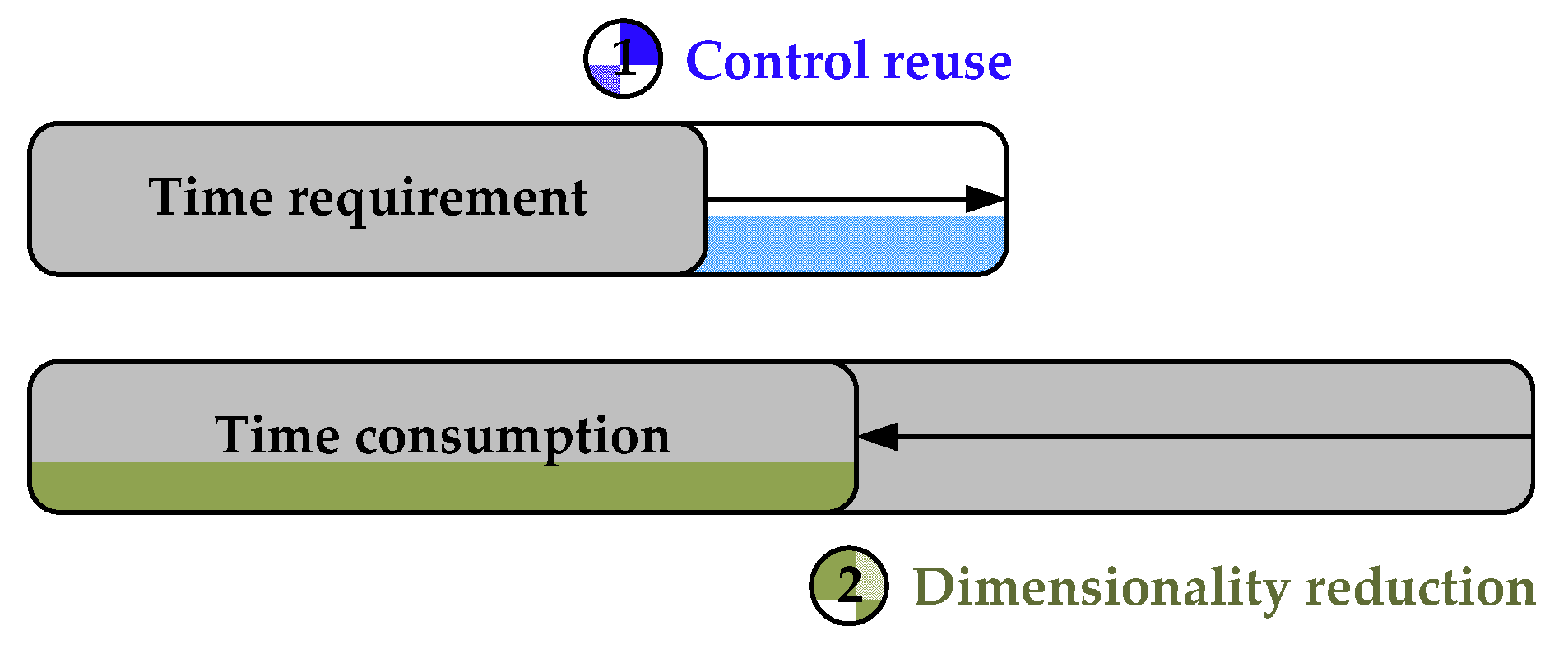
• Parallel computing method for trajectory tube computation: This paper presents a novel method for solving discrete trajectory tubes that simplifies the solution process by eliminating temporal correlations between tubes at different states. This approach enables the efficient parallel processing of trajectory tubes at different state points.
• Dimensionality reduction technique for TRCC of fixed-wing UAVs: Efficient dimensionality reduction techniques, including decoupling and stepwise approaches, are proposed to address higher fast-solving requirements according to fixed-wing UAV characteristics. These techniques are incorporated into a fast TRCC algorithm to enhance online applications.

The structure of this paper is organized as follows. Section 2 provides a detailed description of the methodology for TRCC. Techniques for fast TRCC are presented in Section 3. Section 4 includes simulations and evaluations. Finally, Section 5 presents the conclusions.

2. TRCC Algorithm Based on Discrete Trajectory Tubes

The nonlinear robust control of fixed-wing Unmanned Aerial Vehicles (UAVs) encompasses nonlinear nominal control and Robust Compensation Control (RCC), as shown in Figure 1. The trajectory tube represents the reachable set of actual trajectories for a UAV under disturbance. A smaller tube indicates that the actual trajectories closely approximate the ideal trajectory, thereby demonstrating a higher level of robustness. Consequently, the trajectory tube serves as a quantitative indicator to guide the design of RCC, known as Tube-based RCC (TRCC). Therefore, this section begins by presenting a calculation method for discrete trajectory tubes (step 1 in Figure 1) and subsequently introduces the TRCC method based on this robustness indicator (step 2 in Figure 1).

2.1. Discrete Trajectory Tube Calculation Method

At time step t, for a nonlinear UAV, the relationship between the nominal state $s_t$, the nominal control $a_t$, and the next state $s_{t+1}$ can be described as follows:

$$s_{t+1}-s_t=f\left(s_t,a_t\right)$$

(1)

Under the influence of disturbances, the actual state of the UAV is denoted as ${\overline{s}}_t$. The state error, ${\widehat{s}}_t={\overline{s}}_t-s_t$, can be defined accordingly. Thus, the relationship between the current state error ${\widehat{s}}_t$ and the subsequent state error ${\widehat{s}}_{t+1}$ can be expressed as:

$${\widehat{s}}_{t+1}-{\widehat{s}}_t=f\left(s_t+{\widehat{s}}_t,a_t\right)-f\left(s_t,a_t\right)$$

(2)

The initial set of disturbances is defined as ${\mathcal{P}}_t^0$. When ${\widehat{s}}_t\in {\mathcal{P}}_t^0$, the reachable set ${\mathcal{P}}_{t+1}$ for the next state can be determined by ${\widehat{s}}_{t+1}\in {\mathcal{P}}_{t+1}$. The combination of ${\mathcal{P}}_t^0$ and ${\mathcal{P}}_{t+1}$ constitutes the trajectory tube at time step t, as shown in Figure 2. Due to the uncertainty in the shapes of ${\mathcal{P}}_t^0$ and ${\mathcal{P}}_{t+1}$, the calculation of the trajectory tube becomes more challenging. To overcome this, the external ellipsoids of ${\mathcal{P}}_t^0$ and ${\mathcal{P}}_{t+1}$ are employed to alleviate the computational complexity. Consequently, the trajectory tube ${\mathcal{T}}_t$ used in practice is defined as the region formed by connecting the external ellipsoids ${\mathcal{E}}_t^0$ and ${\mathcal{E}}_{t+1}$ of ${\mathcal{P}}_t^0$ and ${\mathcal{P}}_{t+1}$, respectively.

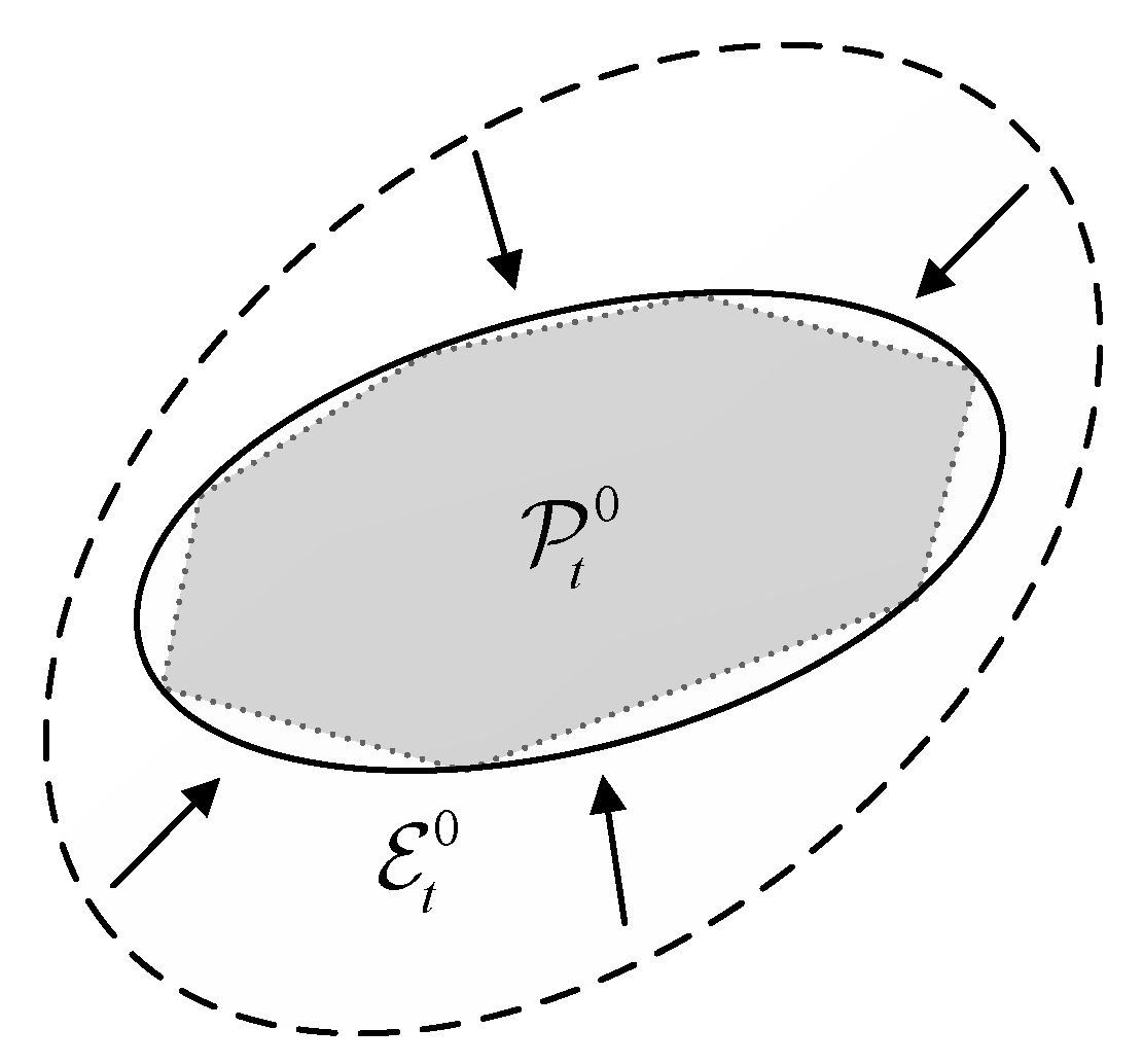
2.1.1. Initial Ellipsoid Calculation

The initial ellipsoid can be defined as ${\mathcal{E}}_t^0=\left\{{\widehat{s}}_t|0\le e_t^0\left({\widehat{s}}_t\right)\le {\rho }_t^0\right\}$, where $e_t^0$ represents the shape of the ellipsoid and ${\rho }_t^0$ represents its size. For solving the initial ellipsoid, $e_t^0$ and ${\rho }_t^0$ are iteratively optimized, and the area of the initial ellipsoid $size\left({\mathcal{E}}_t^0\right)$ can be gradually decreased while ensuring that ${\mathcal{E}}_t^0$ contains ${\mathcal{P}}_t^0$. As shown in Figure 3, the ${\mathcal{E}}_t^0$ gradually approaches the external ellipsoid of ${\mathcal{P}}_t^0$.

The initial error set ${\mathcal{P}}_t^0$ is assumed to be a semi-algebraic set that can be described by $N_t$ polynomial inequalities, denoted as ${\mathcal{P}}_t^0=\left\{{\widehat{s}}_t|g_{t,i}({\widehat{s}}_t)\ge 0,\forall i=1,2,\dots ,N_t\right\}$. Consequently, the optimization problem for finding ${\mathcal{E}}_t^0$ can be formulated as follows:

$$\begin{array}{ll}\underset{e_t^0,{\rho }_t^0}{\min }\hfill & size\left({\mathcal{E}}_t^0\right)\hfill \\ \mathrm{s}.\mathrm{t}.\hfill & g_{t,i}({\widehat{s}}_t)\ge 0,\forall i=1,2,\dots ,N_t\Rightarrow 0\le e_t^0\left({\widehat{s}}_t\right)\le {\rho }_t^0\hfill \end{array}$$

(3)

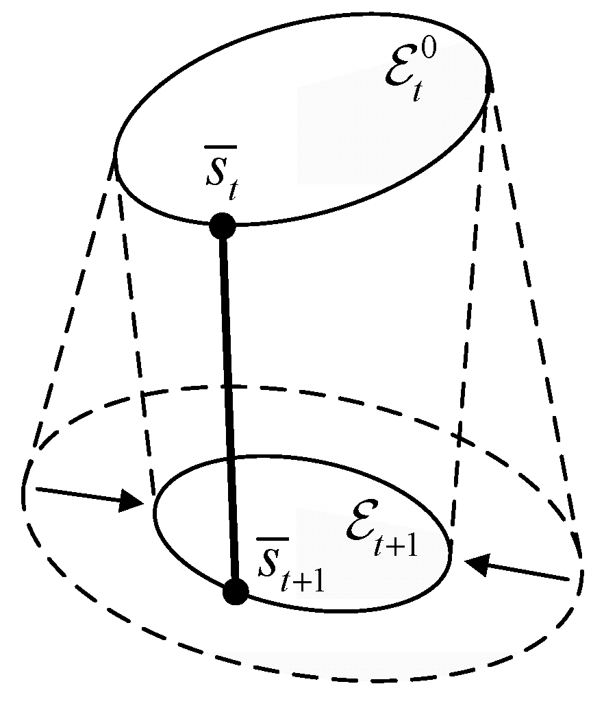
2.1.2. Terminal Ellipsoid Calculation

Similarly, the terminal ellipsoid can be defined as ${\mathcal{E}}_{t+1}=\left\{{\widehat{s}}_{t+1}|0\le e_{t+1}\left({\widehat{s}}_{t+1}\right)\le {\rho }_{t+1}\right\}$. For all initial states located on the initial ellipsoid, the terminal ellipsoid is determined as the smallest ellipsoid that contains the next state. Through the iterative optimization of $e_{t+1}$ and ${\rho }_{t+1}$, the area of the terminal ellipsoid $size\left({\mathcal{E}}_{t+1}\right)$ gradually decreases while maintaining $e_{t+1}\left({\widehat{s}}_{t+1}\right)\le {\rho }_{t+1}$. This approach gives the solution method of the ${\mathcal{E}}_{t+1}$, as depicted in Figure 4.

However, $e_{t+1}\left({\widehat{s}}_{t+1}\right)$ includes all four decision variables ($e_t^0$, ${\rho }_t^0$, $e_{t+1}$, and ${\rho }_{t+1}$), which can present challenges in terminal ellipsoid solving. Hence, the constraint $e_{t+1}\left({\widehat{s}}_{t+1}\right)\le {\rho }_{t+1}$ is converted into an incremental form, $e_t^0\left({\widehat{s}}_t\right)+d{e}_t^0\left({\widehat{s}}_t\right)\le {\rho }_t^0+d{\rho }_t^0$. Additionally, because of $e_t^0\left({\widehat{s}}_t\right)={\rho }_t^0$, the constraint is further transformed into $d{e}_t^0\left({\widehat{s}}_t\right)\le d{\rho }_t^0$, where the increment can be approximated as follows:

$$\left\{\begin{array}{ll}d{e}_t^0\left({\widehat{s}}_t\right)& =\frac{\partial e_t^0}{\partial {\widehat{s}}_t}\times \frac{d{\widehat{s}}_t}{dt}+\frac{\partial e_t^0}{\partial t}\\ & \approx \frac{\partial e_t^0}{\partial {\widehat{s}}_t}\times \frac{{\widehat{s}}_{t+1}-{\widehat{s}}_t}{\Delta t}+\frac{e_{t+1}-e_t^0}{\Delta t}\\ d{\rho }_t^0& \approx \frac{{\rho }_{t+1}-{\rho }_t^0}{\Delta t}\end{array}\right.$$

(4)

In addition, when considering model uncertainties ${\sigma }_t$, the $f\left({\widehat{s}}_t,a_t\right)$ should be modified to $f\left({\widehat{s}}_t,a_t,{\sigma }_t\right)$. Similar to disturbances on the state, model uncertainties can also be described by a semi-algebraic set: ${\mathcal{W}}_t=\left\{{\sigma }_t|g_{\sigma ,t,j}({\sigma }_t)\ge 0,\forall j=1,2,\dots ,N_{\sigma }\right\}$. Hence, the optimization problem for finding ${\mathcal{E}}_{t+1}$ can be formulated as follows:

$$\begin{array}{ll}\underset{e_{t+1},{\rho }_{t+1}}{\min }\hfill & size\left({\mathcal{E}}_{t+1}\right)\hfill \\ \mathrm{s}.\mathrm{t}.\hfill & e_t^0\left({\widehat{s}}_t\right)={\rho }_t^0,g_{\sigma ,t,j}({\sigma }_t)\ge 0,\forall j=1,2,\dots ,N_{\sigma }\Rightarrow d{e}_t^0\left({\widehat{s}}_t\right)\le d{\rho }_t^0\hfill \end{array}$$

(5)

By combining the solution methods for ${\mathcal{E}}_t^0$ and ${\mathcal{E}}_{t+1}$, as given in Equations (3) and (5), respectively, the calculation method for ${\mathcal{T}}_t$ can be derived.

2.2. Sum-of-Squares Programming

Sum-of-Squares Programming (SOSP) can be utilized to verify the validity of a conditional statement [26,28]. The SOSP methodology entails converting the conditional statement into an equivalent polynomial, and its validity is established based on the non-negativity of this polynomial. Moreover, the SOSP method verifies the non-negativity of the polynomial by examining its representability as a sum of squares. Incorporating the SOSP method necessitates adjustments to the constraints, optimization variables, and optimization objectives specified in Equations (3) and (5).

2.2.1. Constraints

Consider the conditional statement $g_{t,i}({\widehat{s}}_t)\ge 0,\forall i=1,2,\dots ,N_t\Rightarrow 0\le e_t^0\left({\widehat{s}}_t\right)\le {\rho }_t^0$ in Equation (3). It is assumed that a set of non-negative multiplier polynomials $L_{t,i} \left(i=1,2,\dots ,N_t\right)$ exists, ensuring that the constructed polynomial ${\rho }_t^0-e_t^0\left({\widehat{s}}_t\right)-{\displaystyle {\sum }_{i=1}^{N_t}{L}_{t,i}({\widehat{s}}_t)g_{t,i}({\widehat{s}}_t)}$ is non-negative. Therefore, when the condition on the left-hand side of “$\Rightarrow$” holds, it can be inferred that ${\rho }_t^0-e_t^0\left({\widehat{s}}_t\right)$ is non-negative, signifying the validity of the conclusion on the right-hand side of “$\Rightarrow$”. By employing the SOSP approach, the constraint in Equation (3) can be modified as follows:

$$\left\{\begin{array}{l}{\rho }_t^0-e_t^0\left({\widehat{s}}_t\right)-{\displaystyle {\sum }_{i=1}^{N_t}{L}_{t,i}({\widehat{s}}_t)g_{t,i}({\widehat{s}}_t)} \mathrm{is} \mathrm{SOS},\hfill \\ L_{t,i}({\widehat{s}}_t) \mathrm{are} \mathrm{SOS}, \forall i=1,2,\dots ,N_t\hfill \end{array}\right.$$

(6)

Similarly, the constraint in Equation (5) can be modified as follows:

$$\left\{\begin{array}{l}d{\rho }_t^0-d{e}_t^0\left({\widehat{s}}_t\right)-\left(e_t^0\left({\widehat{s}}_t\right)-{\rho }_t^0\right)L_t({\widehat{s}}_t)-{\displaystyle {\sum }_{j=1}^{N_{\sigma }}{L}_{\sigma ,t,j}({\widehat{s}}_t)g_{\sigma ,t,j}({\sigma }_t)} \mathrm{is} \mathrm{SOS},\hfill \\ L_{\sigma ,t,j}({\widehat{s}}_t) \mathrm{are} \mathrm{SOS}, \forall j=1,2,\dots ,N_{\sigma }\hfill \end{array}\right.$$

(7)

In addition, in the SOSP, it is necessary for all functions within the constraints to be represented as polynomial functions. Consequently, the Taylor expansion of $f\left({\widehat{s}}_t,a_t,{\sigma }_t\right)$ is employed instead of the original dynamics in the calculation of $d{e}_t^0\left({\widehat{s}}_t\right)$, as stated in Equation (7). Typically, utilizing a third-order Taylor expansion guarantees adherence to computational error requirements [27].

2.2.2. Optimization Variables

In Equation (3), the initial ellipsoid function $e_t^0$ can be represented as a quadratic function with respect to ${\widehat{s}}_t$, denoted as $e_t^0\left({\widehat{s}}_t\right)={\widehat{s}}_t^T{E}_t^0{\widehat{s}}_t$, where $E_t^0$ is a semi-positive definite matrix. Similarly, a semi-positive definite matrix $E_{t+1}$ can be introduced to describe the terminal ellipsoid function $e_{t+1}$. Consequently, the optimization variables are transformed into $E_t^0$, ${\rho }_t^0$, $E_{t+1}$, and ${\rho }_{t+1}$. Furthermore, the optimization variables should include the non-negative multiplier polynomials in the constraints.

2.2.3. Optimization Objectives

In Equation (3), the objective function $size\left({\mathcal{E}}_t^0\right)={\rho }_t^0/\left|E_t^0\right|$ is obtained based on the quadratic expression of the ellipsoid. Similarly, the objective function in Equation (5) is denoted as $size\left({\mathcal{E}}_t{}_{+1}\right)={\rho }_t{}_{+1}/\left|E_t{}_{+1}\right|$.

Taking $size\left({\mathcal{E}}_t^0\right)$ as an example, it is necessary to modify the objective function to $size\left({\mathcal{E}}_t^0\right)={\rho }_t^0$ since the SOSP can only handle linear objective functions. Furthermore, in order to account for the joint reduction of ${\rho }_t^0$ and $\left|E_t^0\right|$, and ensure the feasibility of the optimization problem, the constraints on $E_t^0$ need to be augmented. Therefore, an additional constraint $h^{\mathrm{T}}\left(E_t^0-E_t^{\mathrm{R}}\right)h\ge 0$, $\forall h\ne 0$ is introduced to restrict the unbounded reduction of $\left|E_t^0\right|$ during the optimization calculation. Here, $E_t^{\mathrm{R}}$ represents an initial feasible solution for $E_t^0$. The solution for $E_t^0$ can be obtained by solving the Hamilton–Jacobi–Bellman (HJB) differential equation, and an initial feasible solution can be provided by utilizing the Riccati algebraic equation, which is a simplification of the HJB differential equation under linear conditions [29]. Thus, $E_t^{\mathrm{R}}$ can be determined by the following algebraic equation:

$$E_t^{\mathrm{R}}A\left(s_t\right)+A^{{\rm T}}\left(s_t\right)E_t^{\mathrm{R}}+Q-E_t^{\mathrm{R}}B\left(s_t\right)R^{-1}{B}^{{\rm T}}\left(s_t\right)E_t^{\mathrm{R}}=0,$$

(8)

where matrices A and B represent the state and control matrices, respectively, which are obtained by linearizing equations f at time t. The weight matrices Q and R are diagonal matrices, and their selection is determined by the initial disturbance of the various states. Specifically, the weight values on the diagonal of the weight matrix are chosen to be larger for states with larger initial disturbances.

Similarly, the objective function in Equation (5) needs to be modified to $size\left({\mathcal{E}}_t{}_{+1}\right)={\rho }_t{}_{+1}$, and the constraint $h^{\mathrm{T}}\left(E_{t+1}-E_{t+1}^{\mathrm{R}}\right)h\ge 0$, $\forall h\ne 0$ should be added.

With the incorporation of the SOSP, the mathematical model for the optimization calculation of the initial ellipsoid, as depicted in Equation (3), can be transformed into the following form by considering the adjusted constraints, optimization variables, and objective functions:

$$\begin{array}{ll}\underset{E_t^0,{\rho }_t^0,L_{t,i}}{\min }\hfill & {\rho }_t^0\hfill \\ \mathrm{s}.\mathrm{t}.\hfill & {\rho }_t^0-e_t^0\left({\widehat{s}}_t\right)-{\displaystyle {\sum }_{i=1}^{N_t}{L}_{t,i}({\widehat{s}}_t)g_{t,i}({\widehat{s}}_t)} \mathrm{is} \mathrm{SOS},\hfill \\ \hfill & L_{t,i}({\widehat{s}}_t) \mathrm{are} \mathrm{SOS}, \forall i=1,2,\dots ,N_t,\hfill \\ \hfill & h^{\mathrm{T}}\left(E_t^0-E_t^{\mathrm{R}}\right)h\ge 0, \forall h\ne 0\hfill \end{array}$$

(9)

In addition, the mathematical model for the optimization calculation of the initial ellipsoid, as shown in Equation (5), can be transformed into the following form:

$$\begin{array}{ll}\underset{\begin{array}{c}{E}_{t+1},{\rho }_{t+1},L_t,L_{\sigma ,t,j}\end{array}}{\min }\hfill & {\rho }_{t+1}\hfill \\ \mathrm{s}.\mathrm{t}.\hfill & \mathrm{d}{\rho }_t^0-\mathrm{d}{e}_t^0\left({\widehat{s}}_t\right)-\left(e_t^0\left({\widehat{s}}_t\right)-{\rho }_t^0\right)L_t({\widehat{s}}_t)-{\displaystyle {\sum }_{j=1}^{N_{\sigma }}{L}_{\sigma ,t,j}({\widehat{s}}_t)g_{\sigma ,t,j}({\sigma }_t)} \mathrm{is} \mathrm{SOS},\hfill \\ \hfill & L_{\sigma ,t,j}({\widehat{s}}_t) \mathrm{are} \mathrm{SOS}, \forall j=1,2,\dots ,N_{\sigma },\hfill \\ \hfill & h^{\mathrm{T}}\left(E_{t+1}-E_{t+1}^{\mathrm{R}}\right)h\ge 0, \forall h\ne 0\hfill \end{array}$$

(10)

In summary, by sequentially solving Equations (9) and (10) for a specified range of disturbances, it is feasible to calculate the discrete trajectory tube at the desired state point.

2.3. TRCC Algorithm

To strengthen the robustness of the nominal control $a_t$ against a specified range of disturbances, a polynomial TRCC command ${\widehat{a}}_t\left(\widehat{s}\right)$ is introduced. By incorporating this compensation control, Equation (2) can be modified as follows:

$${\widehat{s}}_{t+1}-{\widehat{s}}_t=f\left(s_t+{\widehat{s}}_t,a_t+{\widehat{a}}_t\left({\widehat{s}}_t\right)\right)-f\left(s_t,a_t\right)$$

(11)

The trajectory tube is utilized as a quantitative indicator to guide the design of TRCC. The feedback control command is optimized to minimize the trajectory tube within a specified range of disturbances, aiming to enhance the robustness of the UAV. Consequently, the TRCC command polynomial is introduced as an optimization variable in the calculation of the terminal ellipsoid, as illustrated in Equation (10).

The magnitude of the compensation control command is constrained by the available control capacity of the UAV after incorporating the nominal control. Therefore, it is necessary to include constraints on the magnitude of the compensation control command in the process of solving for TRCC, as detailed below:

$$e_t^0\left({\widehat{s}}_t\right)\le {\rho }_t^0\Rightarrow a_{\min }\le a_t+{\widehat{a}}_t\left(\widehat{s}\right)\le a_{\max },$$

(12)

where a_max and a_min represent the upper and lower bounds of the control, respectively.

By employing the SOSP method, the conditional statement in Equation (12) can be modified as follows:

$$\left\{\begin{array}{c}{\rho }_t^0-e_t^0\left({\widehat{s}}_t\right)-\left(a_{k,\max }-\left(a_{k,t}+{\widehat{a}}_{k,t}\right)\right)L_{t,au,k}({\widehat{s}}_t) \mathrm{is} \mathrm{SOS},\\ {\rho }_t^0-e_t^0\left({\widehat{s}}_t\right)-\left(\left(a_{k,t}+{\widehat{a}}_{k,t}\right)-a_{k,\min }\right)L_{t,al,k}({\widehat{s}}_t) \mathrm{is} \mathrm{SOS},\end{array}\right.$$

(13)

where $a_t=[a_{1,t},a_{2,t},\cdots ,a_{k,t},\cdots ]$, and $L_{t,au,k}({\widehat{s}}_t)$ and $L_{t,al,k}({\widehat{s}}_t)$ are non-negative multiplier polynomials.

By including the constraints presented in Equation (13), the optimization calculation for the terminal ellipsoid, as illustrated in Equation (10), can be modified to:

$$\begin{array}{ll}\underset{\begin{array}{c}\begin{array}{l}{E}_{t+1},{\rho }_{t+1},{\widehat{a}}_{k,t}\\ L_t,L_{\sigma ,t,j},\\ L_{t,au,k},L_{t,al,k}\end{array}\end{array}}{\min }\hfill & {\rho }_{t+1}\hfill \\ \mathrm{s}.\mathrm{t}.\hfill & \mathrm{d}{\rho }_t^0-\mathrm{d}{e}_t^0\left({\widehat{s}}_t\right)-\left(e_t^0\left({\widehat{s}}_t\right)-{\rho }_t^0\right)L_t\left({\widehat{s}}_t\right)-{\displaystyle {\sum }_{j=1}^{N_{\sigma }}{L}_{\sigma ,t,j}\left({\widehat{s}}_t\right)g_{\sigma ,t,j}({\sigma }_t)} \mathrm{is} \mathrm{SOS},\hfill \\ \hfill & L_{\sigma ,t,j}\left({\widehat{s}}_t\right) \mathrm{are} \mathrm{SOS}, \forall j=1,2,\dots ,N_{\sigma },\hfill \\ \hfill & {\rho }_t^0-e_t^0\left({\widehat{s}}_t\right)-\left(a_{k,\max }-\left(a_{k,t}+{\widehat{a}}_{k,t}\right)\right)L_{t,au,k}\left({\widehat{s}}_t\right) \mathrm{is} \mathrm{SOS},\hfill \\ \hfill & {\rho }_t^0-e_t^0\left({\widehat{s}}_t\right)-\left(\left(a_{k,t}+{\widehat{a}}_{k,t}\right)-a_{k,\min }\right)L_{t,al,k}\left({\widehat{s}}_t\right) \mathrm{is} \mathrm{SOS},\hfill \\ \hfill & L_{t,au,k}\left({\widehat{s}}_t\right),L_{t,al,k}\left({\widehat{s}}_t\right) \mathrm{are} \mathrm{SOS},\hfill \\ \hfill & h^{\mathrm{T}}\left(E_{t+1}-E_{t+1}^{\mathrm{R}}\right)h\ge 0, \forall h\ne 0\hfill \end{array}$$

(14)

Hence, a solution algorithm for TRCC based on a discrete trajectory tube can be derived, as shown in Algorithm 1. Prior to implementing the proposed TRCC algorithm, the nominal state s_t and the nominal control a_t should be given by the nominal nonlinear control.

Algorithm 1 TRCC

In Algorithm 1, each iteration guarantees a decrease in the tube size, forming a monotonically non-increasing sequence. With the tube size bounded below by 0, the convergence of Algorithm 1 can be inferred [27].

3. Fast TRCC for UAV

SOSP transforms the optimization problem of the TRCC command into a semi-definite programming (SDP) problem. The time complexity for solving SDP problems with decision dimensionality n < 10² is O(n^3.5log(1/ε)), where ε represents the required tracking accuracy [30]. The computational time shows a significant increase as the decision dimensionality grows. In the case of fixed-wing UAVs, the solution of TRCC involves addressing high-dimensional SDP, which presents challenges for efficient control command generation.

This section introduces dimensionality reduction techniques aimed at improving solution speed. Two methods for reducing the solving complexity of TRCC in fixed-wing UAVs are considered: decoupling longitudinal and lateral dynamics and stepwise methods. Additionally, control reuse techniques are employed to reduce the real-time requirement in online applications. As shown in Figure 5, by incorporating these techniques, fast compensation control solving can be achieved. This section initially introduces control reuse to reduce real-time requirements and subsequently provides methods for dimensionality reduction.

3.1. Control Reuse

In general, the time interval (beat) Δt_beat for the TRCC command output is set to match the simulation step Δt_step. The calculation time interval Δt_cal for the TRCC command should not exceed Δt_beat and satisfy the condition Δt_cal ≤ Δt_beat = Δt_step, as shown in Figure 6a. By increasing both Δt_beat and Δt_step, the limitation on Δt_cal can be reduced, thereby easing the fast-solving requirement. However, an excessively large Δt_step can compromise the simulation accuracy for UAVs. In this study, compensation control reuse was implemented to enlarge Δt_beat while keeping Δt_step constant, allowing the per-beat compensation control polynomial to be applied to multiple simulation steps. Consequently, the original requirement of Δt_cal ≤ Δt_step was relaxed to Δt_cal ≤ 2Δt_step using a one-step control reuse, as illustrated in Figure 6b. However, control reuse reduces the number of compensation control beats in a multi-step trajectory, resulting in decreased control performance under disturbances compared to no reuse.

3.2. Dimensionality Reduction

3.2.1. Decoupling

For the UAV, the state is defined as s = [V, α, q, θ, β, p, r, ϕ], where V represents the flight velocity, α and β are the angle-of-attack and sideslip angles, respectively; p, q, and r denote the roll, pitch, and yaw angle velocities, respectively; and θ and ϕ represent the pitch and roll angles, respectively. The drone control is denoted by a = [δ_e, δ_th, δ_a, δ_r], where δ_e represents the elevator deflection, δ_th corresponds to the throttle position, δ_a denotes the aileron deflection, and δ_r represents the rudder deflection.

Despite the UAV’s longitudinal and lateral dynamics being coupled, the coupling effects can be disregarded near the nominal trajectory under the action of the nominal control. Considering this assumption, the state used in compensation control calculation, originally consisting of eight dimensions, can be reduced to four dimensions of longitudinal state, s_lon = [V, α, q, θ], and four dimensions of lateral state: s_lat = [β, p, r, ϕ]. Similarly, the four dimensions of control can be reduced to two dimensions of longitudinal control a_lon = [δ_e, δ_th] and two dimensions of lateral control a_lat = [δ_a, δ_r]. Based on the decoupling states and controls, the compensation control calculation can be divided into longitudinal and lateral parts (Algorithm 2). The independence of these two parts allows for parallel computation. With the reduction in state and control dimensions, the TRCC algorithm can be modified as follows:

Algorithm 2 Decoupling TRCC for UAV

Decoupling compensation control affects performance through two factors. Firstly, neglecting longitudinal and lateral coupling results in reduced accuracy and poor control performance. However, simplifying the system to facilitate more accurate control computations under identical hardware and software conditions can ultimately enhance control performance.

3.2.2. Stepwise Method

The stepwise approach involves dividing decision variables into two groups, and sequentially optimizing one while keeping the other fixed. This increases the number of problems but reduces the number of decision variables in each problem, impacting computational time based on the number of variables in the original problem.

In the TRCC algorithm (Algorithm 3), the initial ellipsoid calculation, as depicted in Equation (9), involves three decision variables and is not suitable for variable grouping. In contrast, the terminal ellipsoid calculation, presented in Equation (14), with seven decision variables, suits a stepwise approach for reducing computational time. By grouping the decision variables in Equation (14) into $\{{\rho }_{t+1},{\widehat{a}}_t,L_t,L_{\sigma ,t,j},L_{t,au,k},L_{t,al,k}\}$ and $\{E_{t+1},{\rho }_{t+1}\}$, the optimal solutions for the terminal ellipsoid and compensation control can be obtained separately. This leads to a three-step solution algorithm, modifying the previous two-step approach based on the initial and terminal ellipsoid solutions. The three-step solution algorithm is shown as follows:

Algorithm 3 3-step decoupling TRCC for UAV

In the two-step algorithm (Algorithm 1), the terminal ellipsoid and the compensation control are jointly optimized, resulting in an iterative optimization process for each of them. In contrast, the three-step algorithm optimizes each of them individually only once, which leads to a reduction in calculation accuracy and poor robust control performance. In addition, similar to the two-step algorithm, the three-step algorithm is capable of generating a monotonically non-increasing sequence, ensuring the convergence of the optimization.

4. Simulation Test for Fast TRCC Performance

4.1. UAV Nonlinear Dynamics

4.1.1. Dynamic Equations

In order to conduct a comprehensive simulation and verification analysis of TRCC, this study implemented a continuous nonlinear flight dynamics model for the UAV. This nonlinear model was also utilized in the process of TRCC command calculation; however, it was necessary to discretize the model based on the form of Equation (1).

The quaternion method is utilized in the UAV nonlinear flight dynamics model to prevent singularities that may arise when using the Euler angle method. Equation (15) demonstrates the resulting dynamics equations.

$$\left\{\begin{array}{l}m\left[\begin{array}{c}\dot{u}+qw-rv\\ \dot{v}+ru-pw\\ \dot{w}+pv-qu\end{array}\right]=\left[\begin{array}{c}X+2mg\left(q_1{q}_3-q_0{q}_2\right)\\ Y+2mg\left(q_2{q}_3+q_0{q}_1\right)\\ Z+mg\left(q_0^2-q_1^2-q_2^2+q_3^2\right)\end{array}\right]\hfill \\ \left[\begin{array}{c}L\\ M\\ N\end{array}\right]=\left[\begin{array}{c}{I}_x\dot{p}+(I_z-I_y)qr-I_{zx}\left(pq+\dot{r}\right)\\ I_y\dot{q}+(I_x-I_z)rp+I_{zx}\left(p^2-r^2\right)\\ I_z\dot{r}+(I_y-I_x)pq+I_{zx}\left(qr-\dot{p}\right)\end{array}\right]\hfill \\ \left[\begin{array}{c}{\dot{q}}_0\\ {\dot{q}}_1\\ {\dot{q}}_2\\ {\dot{q}}_3\end{array}\right]=\frac{1}{2}\left[\begin{array}{cccc}0& -p& -q& -r\\ p& 0& r& -q\\ q& -r& 0& p\\ r& q& -p& 0\end{array}\right]\left[\begin{array}{c}{q}_1\\ q_2\\ q_3\\ q_4\end{array}\right]\hfill \end{array}\right.,$$

(15)

where m represents the mass of the body; I_x, I_y, I_z, and I_zx denote the rotational inertia of the body; g represents gravitational acceleration; the vector [u, v, w]^T represents the components of velocity in the body-axis; q₀, q₁, q₂, and q₃ refer to quaternions; and [X, Y, Z]^T and [L, M, N]^T represent the external forces and moments, which primarily account for the influence of aerodynamic forces and engine thrust.

Equation (16) gives the kinematic equations for a UAV in the ground coordinate system.

$$\left\{\begin{array}{l}\left[\begin{array}{l}\dot{x}\\ \dot{y}\\ \dot{z}\end{array}\right]=\left[\begin{array}{ccc}{q}_0^2+q_1^2-q_2^2-q_3^2& 2\left(q_1{q}_2-q_0{q}_3\right)& 2\left(q_1{q}_3+q_0{q}_2\right)\\ 2\left(q_1{q}_2+q_0{q}_3\right)& q_0^2-q_1^2+q_2^2-q_3^2& 2\left(q_2{q}_3-q_0{q}_1\right)\\ 2\left(q_1{q}_3-q_0{q}_2\right)& 2\left(q_2{q}_3+q_0{q}_1\right)& q_0^2-q_1^2-q_2^2+q_3^2\end{array}\right]\left[\begin{array}{c}u\\ v\\ w\end{array}\right]\\ \left[\begin{array}{c}{q}_1\\ q_2\\ q_3\\ q_4\end{array}\right]=\left[\begin{array}{c}\cos \frac{\varphi }{2}\cos \frac{\theta }{2}\cos \frac{\psi }{2}+\sin \frac{\varphi }{2}\sin \frac{\theta }{2}\sin \frac{\psi }{2}\\ \sin \frac{\varphi }{2}\cos \frac{\theta }{2}\cos \frac{\psi }{2}-\cos \frac{\varphi }{2}\sin \frac{\theta }{2}\sin \frac{\psi }{2}\\ \cos \frac{\varphi }{2}\sin \frac{\theta }{2}\cos \frac{\psi }{2}+\sin \frac{\varphi }{2}\cos \frac{\theta }{2}\sin \frac{\psi }{2}\\ \cos \frac{\varphi }{2}\cos \frac{\theta }{2}\mathrm{sins}\frac{\psi }{2}-\sin \frac{\varphi }{2}\sin \frac{\theta }{2}\cos \frac{\psi }{2}\end{array}\right]\end{array}\right.,$$

(16)

where [x, y, z]^T represents the components of the position in the ground-axis, while ψ denotes the yaw angle.

In addition, the velocity and aerodynamic angle of the UAV are determined by the following equation.

$$\left\{\begin{array}{c}V=\sqrt{u^2+v^2+w^2}\\ \alpha =\arctan \left(w/u\right)\\ \beta =\arcsin \left(v/V\right)\end{array}\right.$$

(17)

The UAV’s control inputs include elevator, throttle, aileron, and rudder. The elevator deflection range is [−20°, 20°], the throttle stick position is [0, 1], the aileron deflection range is [−21.5°, 21.5°], and the rudder deflection range is [−30°, 30°].

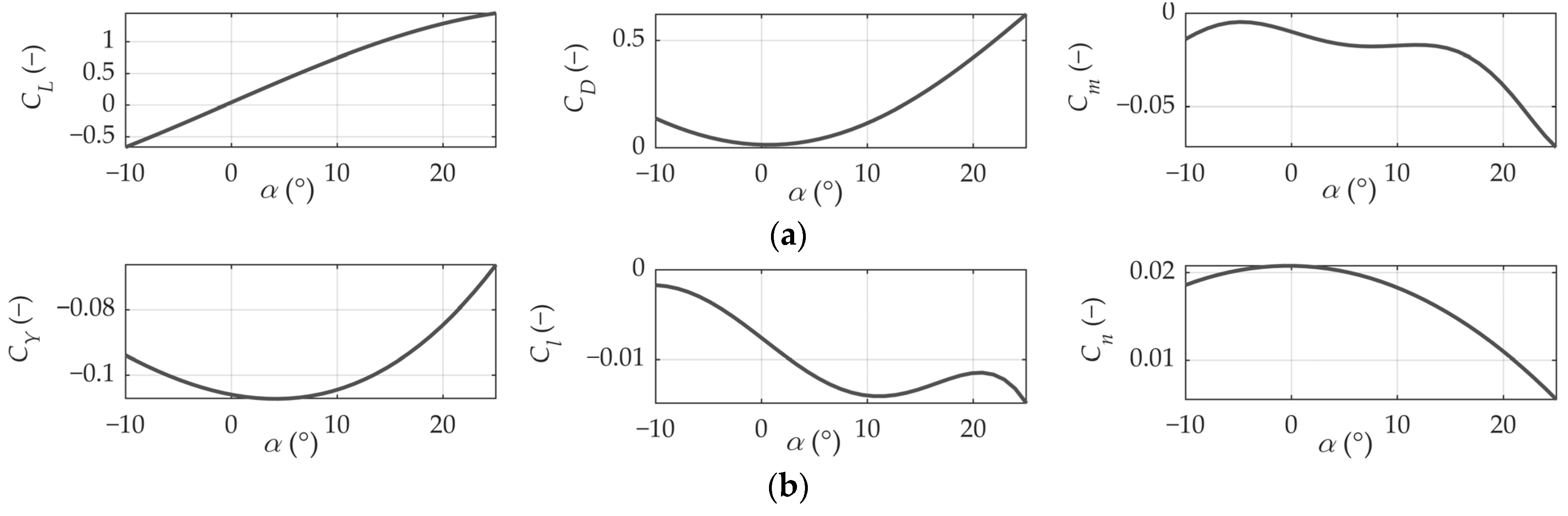
4.1.2. Aerodynamic Characteristics

The nonlinear aerodynamic forces and moments on the UAV can be calculated from the aerodynamic coefficients, denoted as [X_aero, Y_aero, Z_aero, L_aero, M_aero, N_aero]^T = 0.5 × ρ × S × V² × [−C_D, C_Y, −C_L, b × C_l, c × C_m, b × C_n]^T, where ρ is the air density, S is the wing area, b is the aircraft spread length, and c is the average aerodynamic chord length. The variation curves depicting the aerodynamic coefficients mentioned above with respect to the angle-of-attack within the range of −10° to 25° is presented in Figure 7.

4.2. Performance Analysis for TRCC

The performance analysis of the TRCC involves verifying the trajectory tube and conducting simulations of the tracking task under disturbances. The nominal trajectory generated by constant control was used, with its initial state and control outlined in

Table 2. Initial state, control, and disturbance for tube calculation.

Parameter	Value	Parameter	Value
$V$ (m/s)	185	$\widehat{V}$ (m/s)	[−5, 5]
$\alpha$ (°)	19.3	$\widehat{\alpha }$ (°)	[−0.5, 0.5]
$q$ (°/s)	28.2	$\widehat{q}$ (°/s)	[−0.5, 0.5]
$\theta$ (°)	−50.5	$\widehat{\theta }$ (°)	[−1, 1]
$\beta$ (°)	0.7	$\widehat{\beta }$ (°)	[−0.5, 0.5]
$p$ (°/s)	−19.7	$\widehat{p}$ (°/s)	[−1, 1]
$r$ (°/s)	−9.4	$\widehat{r}$ (°/s)	[−0.5, 0.5]
$\varphi$ (°)	0	$\widehat{\varphi }$ (°)	[−1, 1]
$H$ (km)	3	${\delta }_{\mathrm{e}}$ (°)	−5.3
${\delta }_{\mathrm{th}}$ (-)	0.75	${\delta }_{\mathrm{a}}$ (°)	3.0
${\delta }_{\mathrm{r}}$ (°)	0	${\sigma }_m$ (% mmax)	[−5, 5]

. The range of disturbance, determined based on sensor noise, is also presented in Table 2. The flight altitude is denoted by H, while ${\sigma }_m$ represents the mass perturbation in the UAV model.

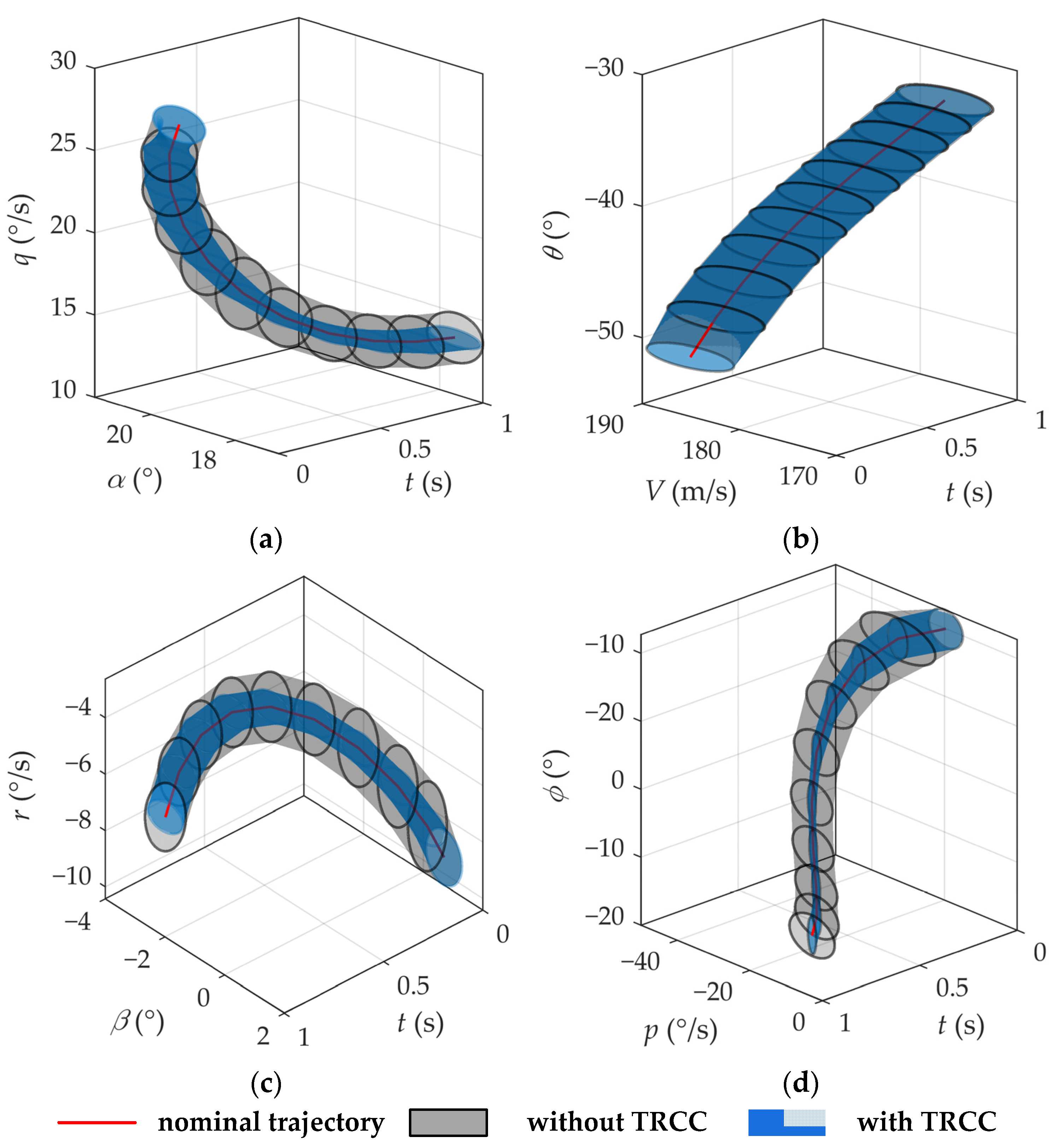
4.2.1. Trajectory Tube

Figure 8 displays the calculated trajectory tubes with and without TRCC. Due to the hyperelliptic characteristic of the trajectory tube in the high-dimensional state, it is essential to project the trajectory tube onto a three-dimensional space composed of any two states and time to observe its shape accurately.

In Figure 8a,b, tube projections for angle-of-attack, velocity, and pitch angles remained unchanged with TRCC, except for a decrease in the pitch angle velocity. Lateral states showed similar variations to longitudinal states, with less variation in sideslip and roll angles, and a significant reduction in yaw and roll angle velocities, as shown in Figure 8c,d. Pitch, roll, and yaw angle velocities are more sensitive to disturbances and exhibit a wider range of variation under disturbances. Hence, TRCC prioritizes the suppression of disturbance effects on angle velocity but fails to fully address angle and velocity disturbances in minimizing the trajectory tube size.

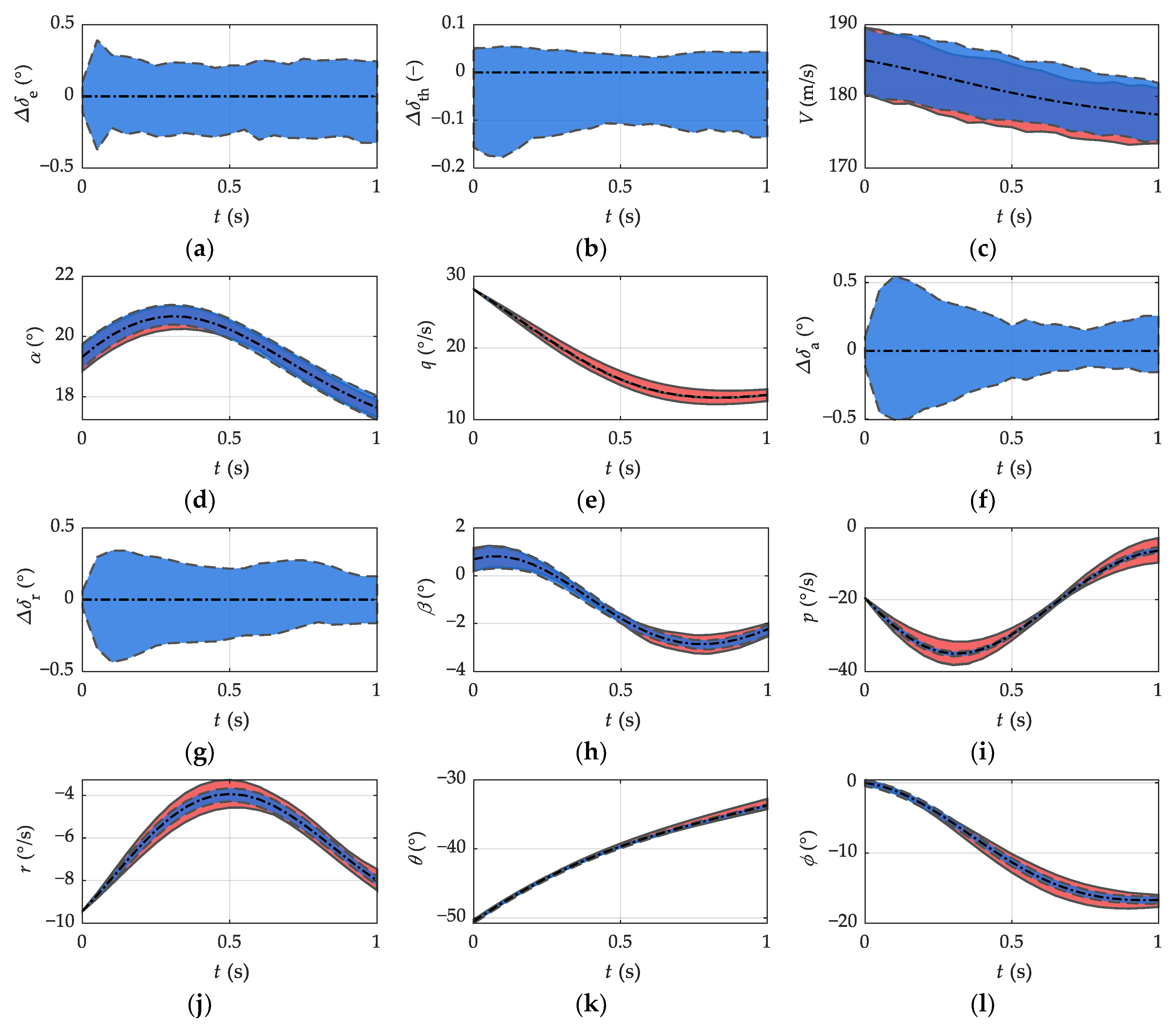
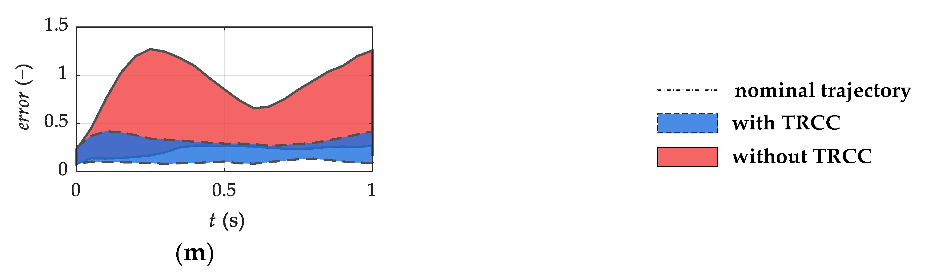
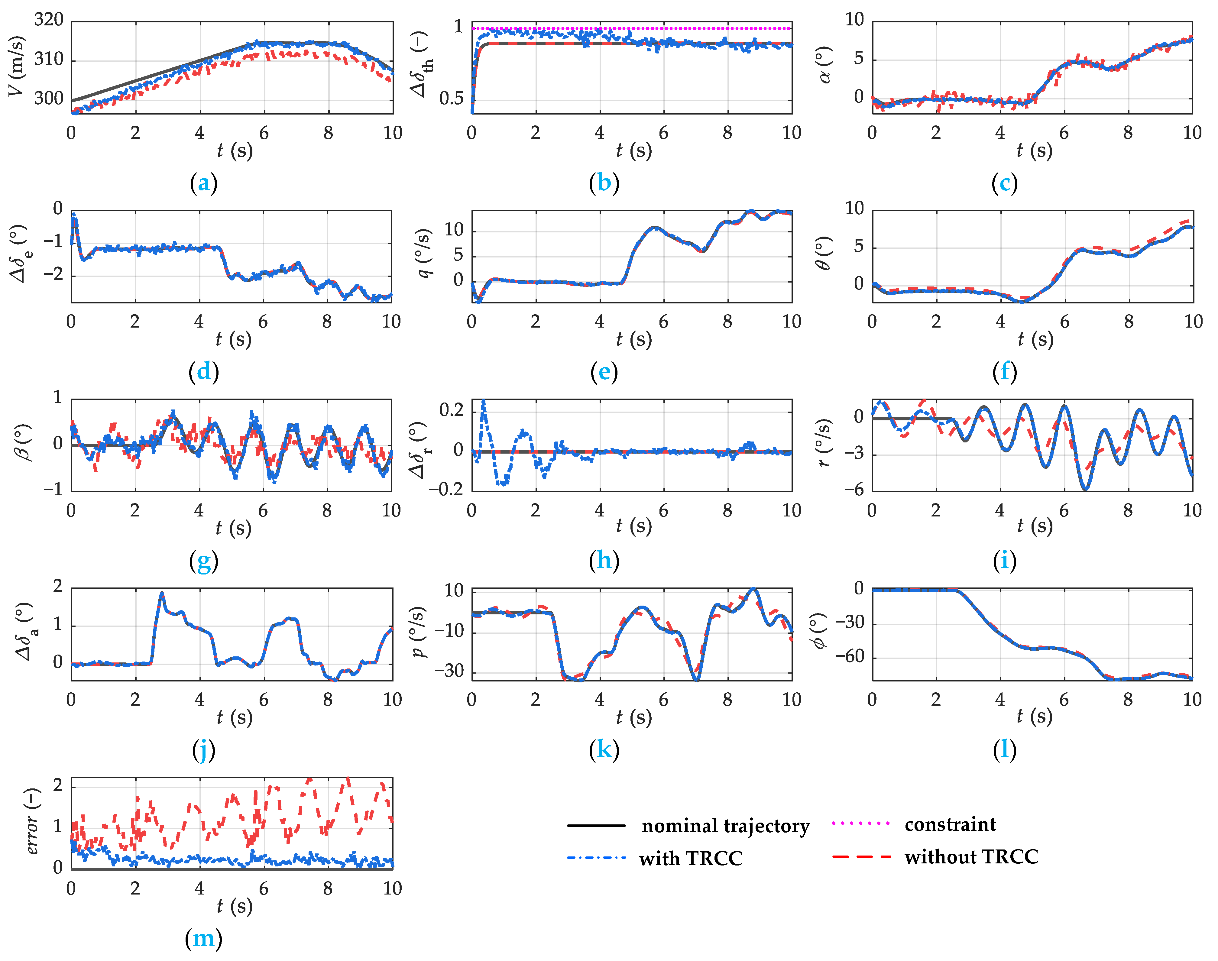
4.2.2. Performance in Tracking Tasks

The effectiveness of TRCC is theoretically demonstrated through a reduction in trajectory tube size. In addition, conducting tracking task simulations under disturbance enables a quantitative analysis of TRCC’s performance disturbance suppression.

Results from 100 tracking task simulations, both with and without TRCC, were recorded separately and displayed in Figure 9. Each simulation considered random combinations of disturbances and modeling inaccuracies generated within the range specified in Table 2. The plotted area in Figure 9 illustrates the upper and lower boundaries of the tracking error for each state influenced by disturbances.

In Figure 9a,b, TRCC produces an elevator increment of −0.2° to 0.2° and a throttle increment of −0.2 to 0.1 under continuous random disturbances. The overall velocity error range exhibited a slight upward shift but maintained a similar magnitude compared to the case without TRCC. Additionally, angle-of-attack errors primarily occurred in the first half of the trajectory. The tracking error ranges for each longitudinal state corresponded to the calculated results for the trajectory tube, as illustrated in Figure 9c–e, as well as in Figure 8a,b.

Furthermore, TRCC produced an aileron increment of −0.5° to 0.5° and a rudder increment of −0.3° to 0.3° under continuous random disturbances, as shown in Figure 9f,g. Aileron and rudder actions resulted in a slight decrease in the error of the sideslip angle during the second half of the trajectory. In addition, the error ranges for roll and yaw angle velocities significantly decreased. The tracking error ranges for each lateral state corresponded to the calculated results for the trajectory tube, as shown in Figure 9h–j, as well as in Figure 8c,d.

In Figure 9k,l, TRCC effectively reduced the pitch angle error during the second half of the trajectory, while the roll angle error was significantly diminished. Although the tracking error range deviated from the calculated trajectory tube, it highlighted the effectiveness of TRCC in mitigating pitch and roll disturbances.

The variable error was introduced to comprehensively describe the state tracking error in the presence of disturbances. It is defined as the root mean square (RMS) of the tracking error across all eight states. Mathematically, it can be expressed as:

$$error=\sqrt{\frac{{\displaystyle \sum e_i^2}}{{\displaystyle \sum i}}}, \left(i=\frac{\widehat{V}}{{10}^2},\widehat{\alpha },\widehat{q},\widehat{\theta },\widehat{\beta },\widehat{p},\widehat{r},\widehat{\varphi }\right),$$

(18)

where the velocity error is divided by 10² to account for the significant magnitude difference compared with other states.

In Figure 9m, without TRCC, the average maximum tracking error (the average upper boundary of the tracking error over time) was 0.93. With TRCC, it decreased to 0.32, a 66% reduction. This demonstrates the effective improvement in UAV robustness achieved by the proposed TRCC in conjunction with nominal control.

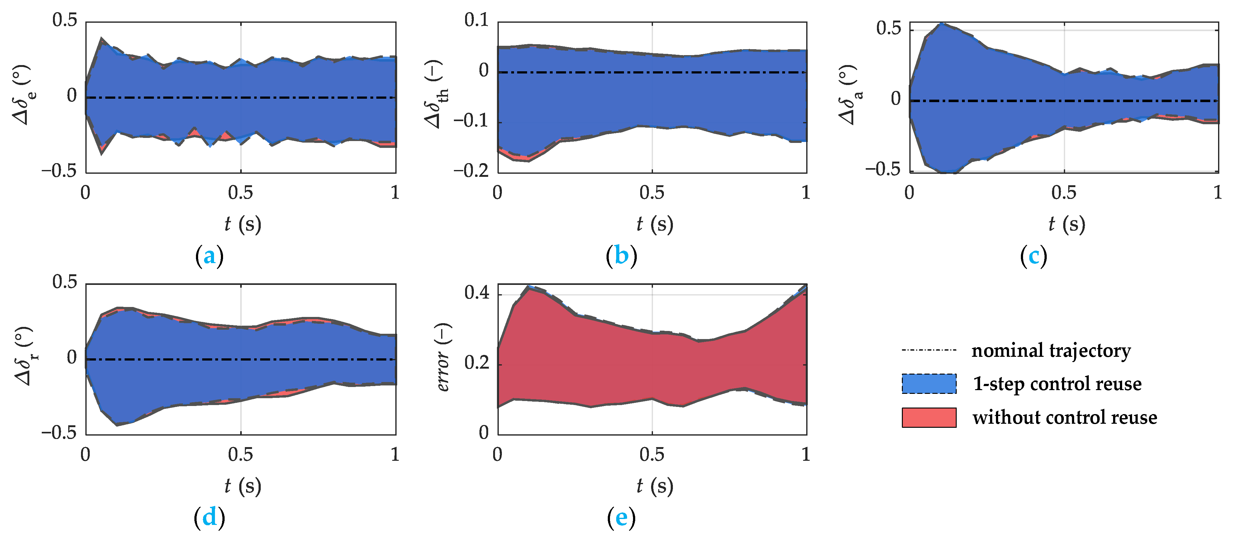
4.3. Performance Analysis for TRCC with Control Reuse

To assess the influence of control reuse, 100 tracking task simulations were conducted. Random combinations of disturbances and modeling errors within the range specified in Table 2 were employed. The simulations compared scenarios without control reuse and with one-step control reuse, as illustrated in Figure 10.

Figure 10a–d demonstrates that one-step control reuse widens the gap between successive TRCC commands, resulting in significant variation during TRCC switching. The elevator increment was particularly affected by the reuse, exhibiting noticeable jaggedness, while the throttle, aileron, and rudder displayed relatively slight jaggedness.

With one-step control reuse, the average maximum tracking error increased from 0.32 to 0.33, resulting in just a 3% increment compared to the case without control reuse, as shown in Figure 10e. Therefore, employing control reuse enables a reduction in fast-solving requirements while still satisfying the robustness requirement.

4.4. Time Consumption and Performance Analysis for Decoupling TRCC

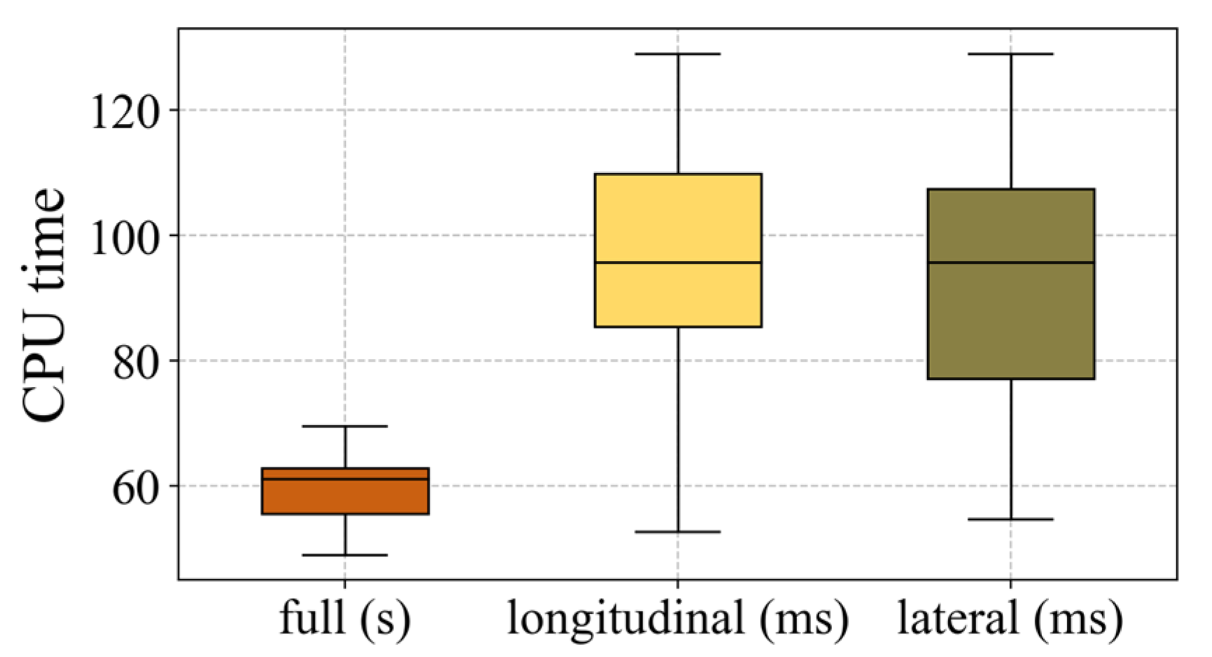
4.4.1. Time Consumption

To analyze the computational time consumption of decoupling TRCC, the algorithms with and without dimensionality reduction were utilized to calculate the TRCC command 100 times. The computational time was recorded, and its distribution is depicted in Figure 11.

The computational time analysis employed an SOSP solver based on the MATLAB R2020a platform SOSTOOLS v4.00 [31] and SEDUMI v1.05 [32]. All analysis results were obtained using an “Intel Xeon Gold 6230” 40-thread CPU (2.10 GHz) with 128GB RAM.

As illustrated in Figure 11, the computational time needed for TRCC is typically in the order of seconds, with a median value of approximately 61 s. This duration falls short of meeting the requirement for rapid generation. However, by employing the decoupling TRCC algorithm, the computation time for solving both the longitudinal and lateral subproblems is reduced to the millisecond range, with medians of around 94 ms and 95 ms, and maximums of about 129 ms and 128 ms, respectively. Hence, the decoupling TRCC algorithm can satisfy the fast generation criteria of 100 ms per beat, although a small number of cases slightly exceed this threshold.

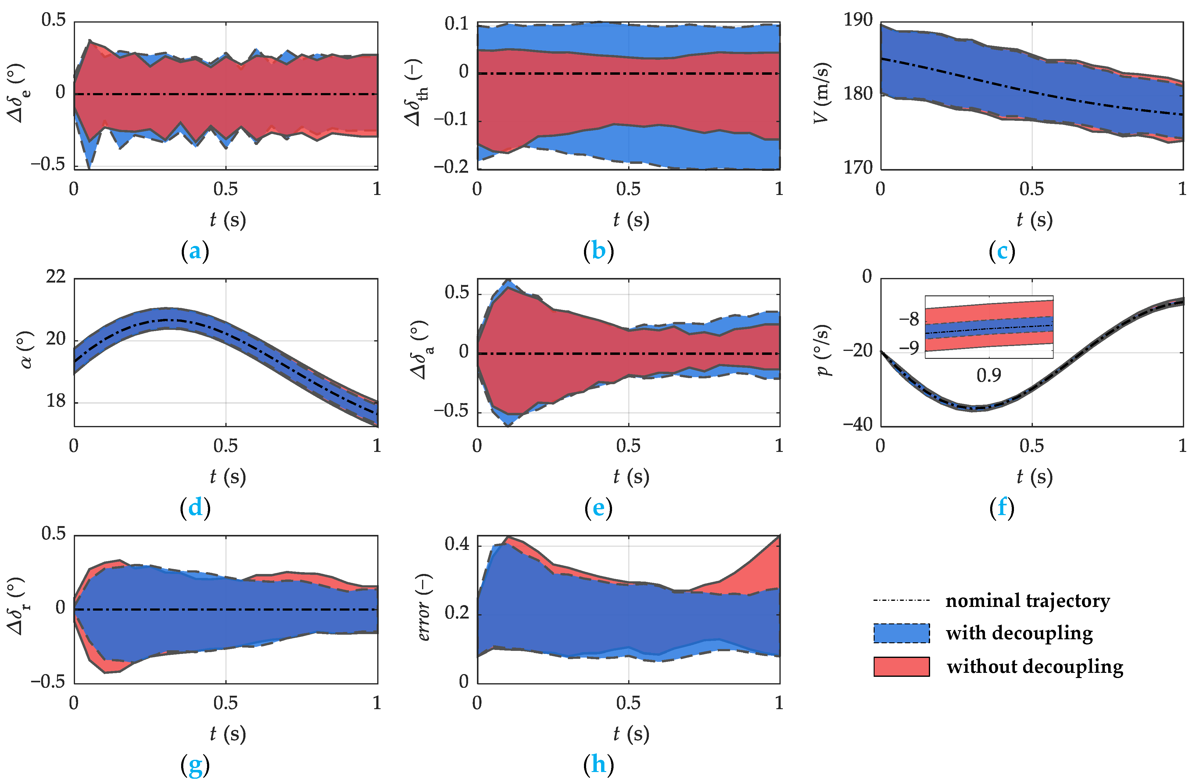
4.4.2. Performance in Tracking Tasks

To assess the influence of decoupling and dimensionality reduction, 100 tracking task simulations were conducted. Random combinations of disturbances and modeling errors within the range specified in Table 2 were employed. The simulations compared scenarios with and without decoupling, as illustrated in Figure 12.

Figure 12a,b demonstrates the increased variation of elevator and throttle when utilizing decoupling TRCC, facilitating a more aggressive suppression of longitudinal disturbances. Consequently, Figure 12c,d exhibits slight reductions in velocity and angle-of-attack errors. Similarly, Figure 12e,f showcases expanded aileron variation, enabling the aggressive reduction of the roll angle velocity error. The variation in the rudder remained unchanged, as depicted in Figure 12g, and no significant differences were observed in other state error responses. Decoupling TRCC reduces the average maximum tracking error from 0.33 to 0.30 when compared to TRCC without decoupling, as shown in Figure 12h.

Therefore, within a given UAV decoupling TRRC algorithm, the simplification of the problem after decoupling significantly enhanced computational accuracy, outweighing the decrease from neglecting longitudinal and lateral coupling. The decoupling TRRC effectively reduced the computational time and improved the control performance.

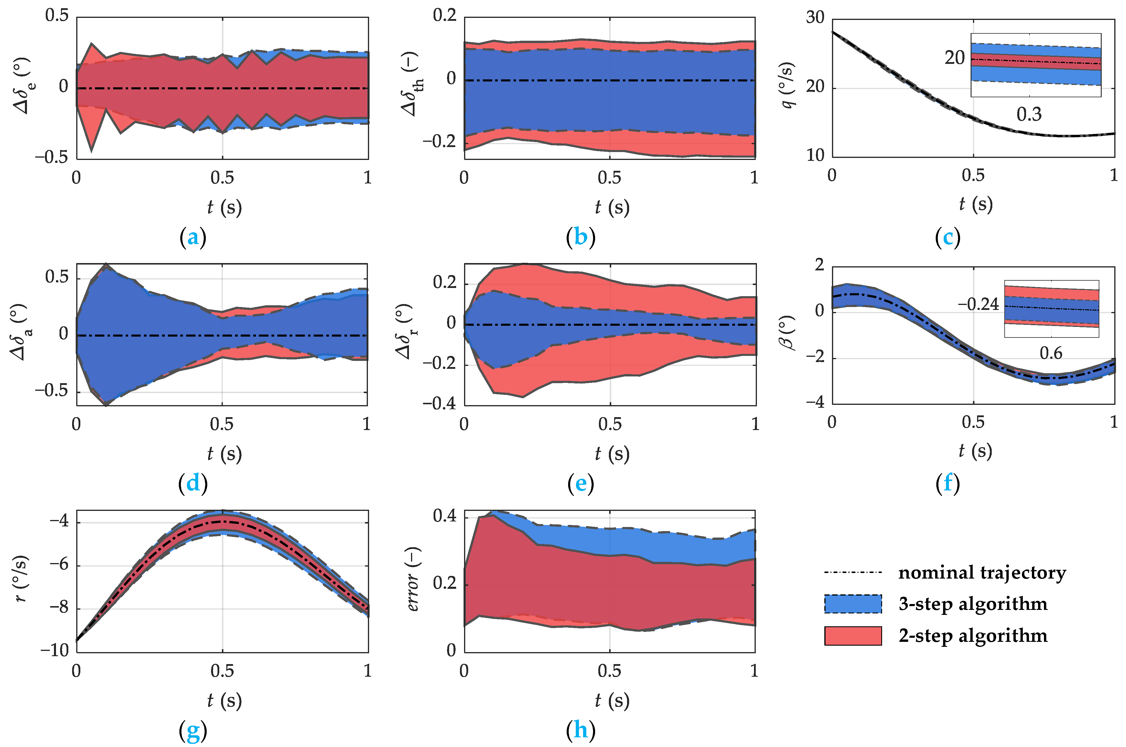
4.5. Time Consumption and Performance Analysis for Stepwise TRCC

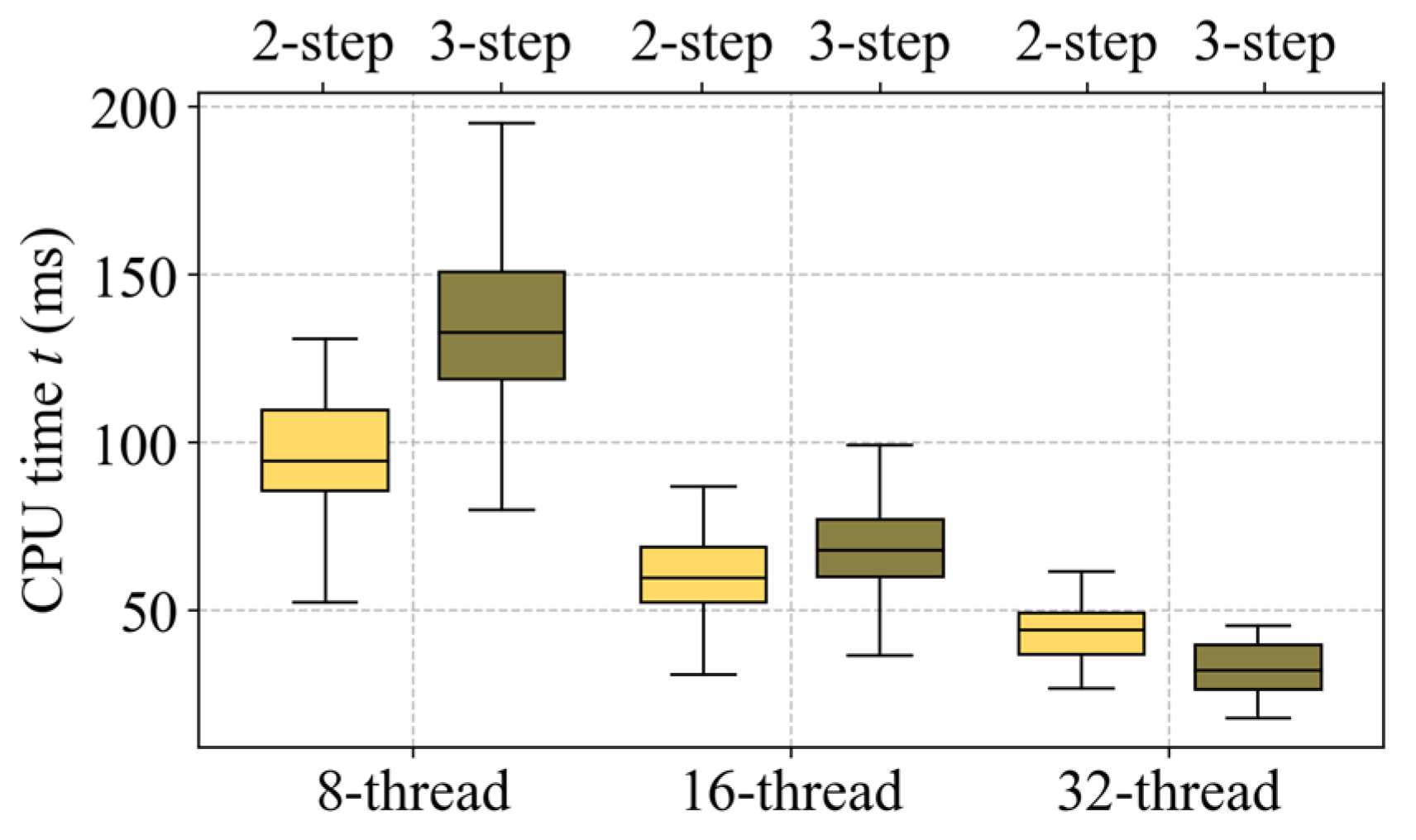
4.5.1. Time Consumption

In addition to the incorporation of the decoupling algorithm, two-step and three-step algorithms were employed to calculate the TRCC command 100 times. The computational time was recorded, and its distribution is depicted in Figure 13.

The median computation times for solving TRCC were approximately 95 ms and 133 ms using the two-step and three-step algorithms, respectively, with eight parallel computing threads. In addition, based on Welch’s t-test at a 5% significance level, three-step algorithms exhibited a significantly higher average computation time than two-step algorithms, by 41.5 ms.

Increasing the number of threads to 16, the median computation times were approximately 60 ms and 68 ms using the two-step and three-step algorithms, respectively. Additionally, based on Welch’s t-test at a 5% significance level, three-step algorithms exhibited a slightly higher average computation time than two-step algorithms, by 7.5 ms.

On further raising the number of threads to 32, the median computation times were approximately 44 ms and 33 ms using the two-step and three-step algorithms, respectively. In addition, based on Welch’s t-test at a 5% significance level, three-step algorithms exhibited a moderately lower average computation time than two-step algorithms, by 10.6 ms. As the number of parallel computation threads increased, the three-step algorithm showed superiority.

4.5.2. Performance in Tracking Tasks

To assess the influence of the stepwise method, 100 tracking task simulations were conducted. Random combinations of disturbances and modeling errors within the range specified in Table 2 were employed. The simulations compared scenarios with two-step and three-step algorithms, as illustrated in Figure 14.

Figure 14a,b shows that the three-step algorithm reduced the variation of the elevator and throttle compared to the two-step algorithm. Hence, this reduction led to ineffective compensation for longitudinal disturbances, increasing the pitch angle velocity error, as shown in Figure 14c. Additionally, the three-step algorithm led to minor aileron variation but significantly reduced the rudder variation, as shown in Figure 14d,e. Therefore, the rudder failed to adequately compensate for lateral disturbances, resulting in increased sideslip angle and yaw angle velocity errors, as shown in Figure 14f,g. Figure 14h demonstrates that the average maximum tracking error increased from 0.30 to 0.37 when employing the three-step algorithm instead of the two-step algorithm. Thus, although the three-step algorithm reduced the computational time, it resulted in an approximately 23% reduction in TRCC performance.

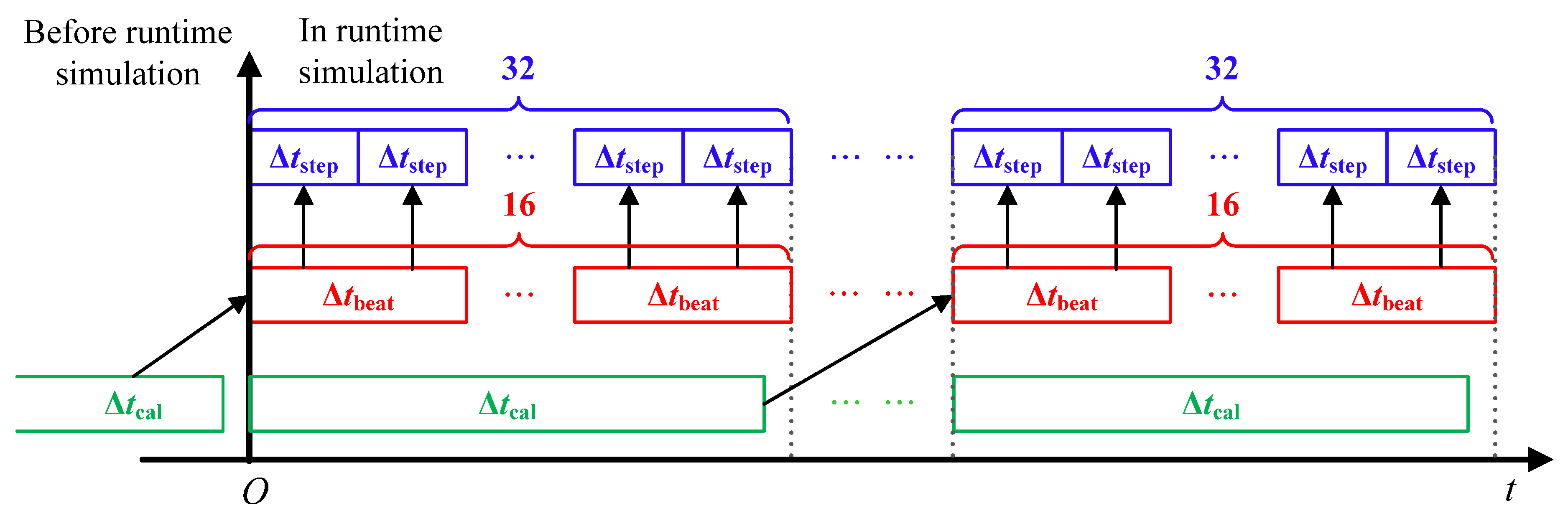
4.6. Runtime Simulation

To validate the real-time performance of the Fast TRCC, a runtime simulation was conducted. The hardware device supported up to 40 parallel computational threads, with 16 threads each used for longitudinal and lateral RCC computation. The computation time analysis (Figure 13) demonstrated a consumption below 100 ms for the 16-thread environment, effectively meeting the 50 ms real-time requirement with a one-step delay. Consequently, the simulation step was set at 50 ms in the runtime simulation. Before initiating the runtime simulation, the TRCC command for the first 16 beats was pre-calculated. Throughout the runtime simulation, the algorithm handles the calculation of RCC commands for the subsequent 16 beats, as depicted in Figure 15. The results of the runtime simulation are presented in Figure 16.

In the runtime test, the velocity initially deviated by 3 m/s, as depicted in Figure 16a. Since the actual velocity was lower than the nominal velocity, TRCC generated a positive throttle compensation to minimize the velocity error. The compensated throttle consistently satisfied the constraint, as illustrated in Figure 16b. Furthermore, TRCC effectively suppressed the measurement noise of the velocity and angle-of-attack through throttle and elevator compensation, reducing the tracking error of pitch angle velocity and pitch angle, as indicated in Figure 16a,f. In addition, in the runtime simulation, an angle-of-attack of 7° was achieved, in which the aerodynamic characteristics presented moderate nonlinearity, as shown in Figure 7.

As shown in Figure 16g, the sideslip angle exhibited an initial deviation of 0.3° and was affected by continuous measurement noise. Consequently, TRCC generated a larger rudder compensation, leading to a reduction in the tracking error for the sideslip angle and yaw angle velocity, as depicted in Figure 16g–i. Although TRCC produced a smaller aileron compensation, it still effectively reduced the tracking error for the roll angle velocity and roll angle, as shown in Figure 16j–l.

The combined tracking error curves, with and without the effect of TRCC, are presented in Figure 16m. To effectively evaluate the control effect of TRCC, the Mean Absolute Error (MAE) and Root Mean Square Error (RMSE) metrics of the tracking error were used [33]. By utilizing TRCC to suppress the effect of initial state deviation and measurement noise, the MAE of the tracking error was reduced from 1.21 to 0.25, and the RMSE decreased from 1.30 to 0.27 after the implementation of TRCC, indicating improved robustness.

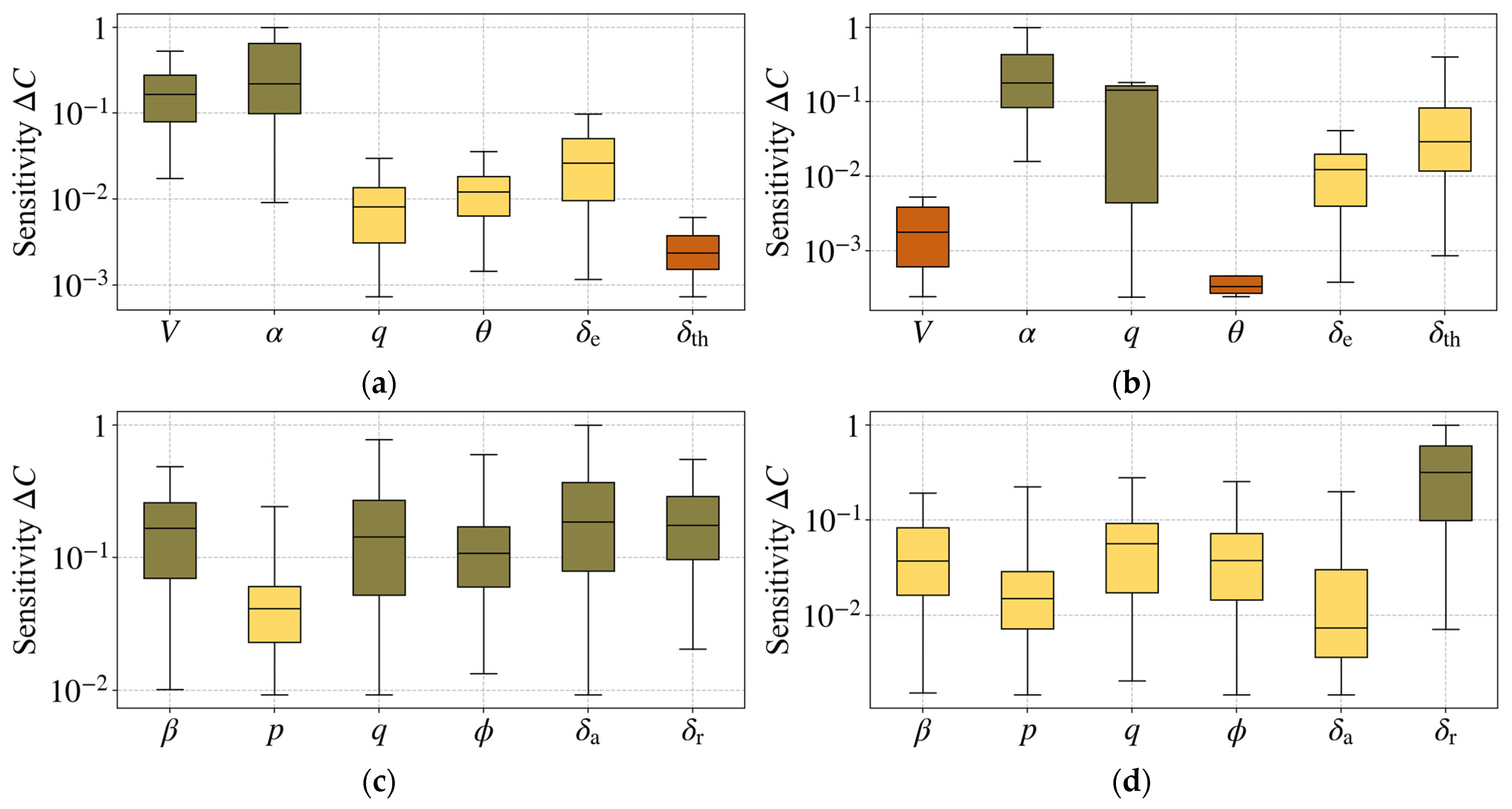
4.7. Sensitivity Analysis

Sensitivity analysis identifies key nominal states and actions affecting the TRCC command. The recalculation of the compensation control command polynomials is conducted only when these key factors experience significant changes, reducing the computational burden of TRCC implementation.

In the sensitivity analysis, two sets of 100 test nominal state and control inputs were randomly sampled within the ranges specified in

Table 3. Range of nominal states and controls for sensitivity analysis.

Parameter	Range	Parameter	Range
$V$ (m/s)	[200, 350]	$\alpha$ (°)	[−10, 25]
$q$ (°/s)	[−30, 30]	$\theta$ (°)	[−60, 60]
$\beta$ (°)	[−10, 10]	$p$ (°/s)	[−50, 50]
$r$ (°/s)	[−10, 10]	$\varphi$ (°)	[−90, 90]
${\delta }_{\mathrm{e}}$ (°)	[−15, 15]	${\delta }_{\mathrm{th}}$ (-)	[0.2, 0.8]
${\delta }_{\mathrm{a}}$ (°)	[−15, 15]	${\delta }_{\mathrm{r}}$ (°)	[−25, 25]

. The sensitivity was determined by computing ΔC = C₁ − C₂, where C₁ and C₂ are the coefficients of the compensation command polynomials obtained under the two sets of test inputs. A larger ΔC indicates that the input has a significant influence on the TRCC command, indicating high sensitivity. The sensitivity analysis results are shown in Figure 17.

In the sensitivity analysis, Welch’s t-tests at a 5% significance level were used to evaluate the differences in average sensitivity ΔC. Figure 17a shows that elevator compensation control had the highest sensitivity to nominal velocity and angle-of-attack, with the average sensitivity at least one order of magnitude higher than other states and controls. Similarly, Figure 17b demonstrates the significant sensitivity of throttle compensation control to the nominal angle-of-attack and pitch angle velocity. Figure 17c indicates comparable average sensitivity results for aileron compensation control across lateral nominal states and controls, except for the roll angle velocity. Lastly, Figure 17d reveals the substantial sensitivity of rudder compensation control to nominal rudder deflection, exceeding other nominal states and controls by at least one order of magnitude.

5. Conclusions

This study introduced a method for calculating a discrete trajectory tube and developed a parallel TRCC algorithm that enhanced robustness by minimizing the tube. Additionally, two efficient methods for solving TRCC commands for UAVs were presented: dimensionality reduction techniques (decoupling and stepwise) and control reuse. Through runtime simulations under external disturbances and dynamic uncertainties, it was verified that the proposed fast TRCC effectively enhances the robustness of UAVs during tracking tasks while satisfying the requirements for fast solving, as supported by the following two key points:

• The TRCC method for UAVs reduces the RMS tracking error by 66% compared to the uncompensated control, significantly enhancing robustness during maneuver trajectory tracking.
• By utilizing one-step reuse, UAV decoupling, and a three-step algorithm, the TRCC fast generation requirement of 50 ms per beat can be achieved in a 16-thread environment. Simulations demonstrate that the fast TRCC method reduces the RMS tracking error by 60% compared to the uncompensated control. However, when subjected to the same range of disturbances, the fast TRCC exhibits an approximate 9% increase in the RMS tracking error compared to the slow nominal TRCC, indicating lower robustness.

In addition, the fast-solving method for trajectory tubes proposed in this paper enables real-time assessment of robustness in nonlinear UAVs. In future work, its application can extend beyond UAV control to benefit trajectory planning and situation assessment, addressing disturbances in practical scenarios.

References

1. Wang, M.; Wang, L.; Yue, T.; Liu, H. Influence of unmanned combat aerial vehicle agility on short-range aerial combat effectiveness. Aerosp. Sci. Technol. 2020, 96, 105534. [Google Scholar] [CrossRef]
2. Pereira, L.A.A.; Pimenta, L.C.A.; Raffo, G.V. MPC Based Feedback-Linearization Strategy of a Fixed-Wing UAV. Automática 2020, 2, 1. [Google Scholar] [CrossRef]
3. Pfeifle, O.; Fichter, W. Cascaded incremental nonlinear dynamic inversion for three-dimensional spline-tracking with wind compensation. J. Guid. Control Dyn. 2021, 44, 1559–1571. [Google Scholar] [CrossRef]
4. Olguin-Roque, J.; Salazar, S.; González-Hernandez, I.; Lozano, R. A Robust Fixed-Time Sliding Mode Control for Quadrotor UAV. Algorithms 2023, 16, 229. [Google Scholar] [CrossRef]
5. Wang, Q.; Wang, W.; Suzuki, S.; Namiki, A.; Liu, H.; Li, Z. Design and implementation of UAV velocity controller based on reference model sliding mode control. Drones 2023, 7, 130. [Google Scholar] [CrossRef]
6. Mothes, F. Trajectory planning in time-varying adverse weather for fixed-wing aircraft using robust model predictive control. Aerospace 2019, 6, 68. [Google Scholar] [CrossRef] [Green Version]
7. Melo, A.G.; Andrade, F.A.A.; Guedes, I.P.; Carvalho, G.F.; Zachi, A.R.L.; Pinto, M.F. Fuzzy gain-scheduling PID for UAV position and altitude controllers. Sensors 2022, 22, 2173. [Google Scholar] [CrossRef] [PubMed]
8. Alsaade, F.W.; Jahanshahi, H.; Yao, Q.; Al-Zahrani, M.S.; Alzahrani, A.S. A new neural network-based optimal mixed H2/H∞ control for a modified unmanned aerial vehicle subject to control input constraints. Adv. Space Res. 2023, 71, 3631–3643. [Google Scholar] [CrossRef]
9. Wan, K.; Gao, X.; Hu, Z.; Wu, G. Robust motion control for UAV in dynamic uncertain environments using deep reinforcement learning. Remote Sens. 2020, 12, 640. [Google Scholar] [CrossRef] [Green Version]
10. Fu, Y.; Zhao, W.; Liu, L. Safe Reinforcement Learning for Transition Control of Ducted-Fan UAVs. Drones 2023, 7, 332. [Google Scholar] [CrossRef]
11. Popov, A.M.; Kostrygin, D.G.; Shevchik, A.A.; Andrievsky, B. Speed-Gradient Adaptive Control for Parametrically Uncertain UAVs in Formation. Electronics 2022, 11, 4187. [Google Scholar] [CrossRef]
12. Lungu, M. Auto-landing of UAVs with variable centre of mass using the backstepping and dynamic inversion control. Aerosp. Sci. Technol. 2020, 103, 105912. [Google Scholar] [CrossRef]
13. Wang, Q.; Namiki, A.; Asignacion, A., Jr.; Li, Z.; Suzuki, S. Chattering Reduction of Sliding Mode Control for Quadrotor UAVs Based on Reinforcement Learning. Drones 2023, 7, 420. [Google Scholar] [CrossRef]
14. Cao, S.; Shen, L.; Zhang, R.; Yu, H.; Wang, X. Adaptive incremental nonlinear dynamic inversion control based on neural network for UAV maneuver. In Proceedings of the 2019 IEEE/ASME International Conference on Advanced Intelligent Mechatronics (AIM), Hong Kong, China, 8–12 July 2019; IEEE: Tampa, FL, USA, 2019. [Google Scholar] [CrossRef]
15. Liu, H.; Lu, G.; Zhong, Y. Robust LQR attitude control of a 3-DOF laboratory helicopter for aggressive maneuvers. IEEE Trans. Ind. Electron. 2012, 60, 4627–4636. [Google Scholar] [CrossRef]
16. Liu, H.; Wang, X.; Zhong, Y. Quaternion-based robust attitude control for uncertain robotic quadrotors. IEEE Trans. Ind. Inform. 2015, 11, 406–415. [Google Scholar] [CrossRef]
17. Mayne, D.Q.; Seron, M.M.; Raković, S.V. Robust model predictive control of constrained linear systems with bounded disturbances. Automatica 2005, 41, 219–224. [Google Scholar] [CrossRef]
18. Raković, S.V.; Kouvaritakis, B.; Findeisen, R.; Cannon, M. Homothetic tube model predictive control. Automatica 2012, 48, 1631–1638. [Google Scholar] [CrossRef]
19. Raković, S.V.; Kouvaritakis, B.; Cannon, M.; Panos, C.; Findeisen, R. Parameterized tube model predictive control. IEEE Trans. Autom. Control 2012, 57, 2746–2761. [Google Scholar] [CrossRef]
20. Mayne, D.Q.; Kerrigan, E.C.; Van Wyk, E.J.; Falugi, P. Tube-based robust nonlinear model predictive control. Int. J. Robust Nonlinear Control 2011, 21, 1341–1353. [Google Scholar] [CrossRef]
21. Moore, J.; Cory, R.; Tedrake, R. Robust post-stall perching with a simple fixed-wing glider using LQR-Trees. Bioinspir. Biomim. 2014, 9, 025013. [Google Scholar] [CrossRef] [Green Version]
22. Majumdar, A.; Ahmadi, A.A.; Tedrake, R. Control design along trajectories with sums of squares programming. In Proceedings of the 2013 IEEE International Conference on Robotics and Automation, Karlsruhe, Germany, 6–10 May 2013; IEEE: Tampa, FL, USA, 2013. [Google Scholar] [CrossRef] [Green Version]
23. Tobenkin, M.M.; Manchester, I.R.; Tedrake, R. Invariant funnels around trajectories using sum-of-squares programming. IFAC Proc. Vol. 2011, 44, 9218–9223. [Google Scholar] [CrossRef]
24. Herbert, S.L.; Bansal, S.; Ghosh, S.; Tomlin, C.J. Reachability-based safety guarantees using efficient initializations. In Proceedings of the 2019 IEEE 58th Conference on Decision and Control (CDC), Nice, France, 11–13 December 2019; IEEE: Tampa, FL, USA, 2019. [Google Scholar] [CrossRef] [Green Version]
25. Seo, H.; Son, C.Y.; Kim, H.J. Fast funnel computation using multivariate Bernstein polynomial. IEEE Robot. Autom. Lett. 2021, 6, 1351–1358. [Google Scholar] [CrossRef]
26. Cunis, T.; Legat, B. Sequential sum-of-squares programming for analysis of nonlinear systems. In Proceedings of the 2023 American Control Conference (ACC), San Diego, CA, USA, 31 May–2 June 2013; IEEE: Tampa, FL, USA, 2013. [Google Scholar] [CrossRef]
27. Majumdar, A.; Tedrake, R. Funnel libraries for real-time robust feedback motion planning. Int. J. Robot. Res. 2017, 36, 947–982. [Google Scholar] [CrossRef]
28. Prajna, S.; Papachristodoulou, A.; Parrilo, P.A. Introducing SOSTOOLS: A general purpose sum of squares programming solver. In Proceedings of the 41st IEEE Conference on Decision and Control, Las Vegas, NV, USA, 10–13 December 2002; IEEE: Tampa, FL, USA, 2002. [Google Scholar] [CrossRef] [Green Version]
29. Mitchell, I.M.; Bayen, A.M.; Tomlin, C.J. A time-dependent Hamilton-Jacobi formulation of reachable sets for continuous dynamic games. IEEE Trans. Autom. Control 2005, 50, 947–957. [Google Scholar] [CrossRef] [Green Version]
30. Waldspurger, I.; d’Aspremont, A.; Mallat, S. Phase recovery, maxcut and complex semidefinite programming. Math. Program. 2015, 149, 47–81. [Google Scholar] [CrossRef] [Green Version]
31. Papachristodoulou, A.; Anderson, J.; Valmorbida, G.; Prajna, S.; Seiler, P.; Parrilo, P.; Peet, M.M.; Jagt, D. SOSTOOLS version 4.00 sum of squares optimization toolbox for MATLAB. arXiv 2013, arXiv:1310.4716. [Google Scholar]
32. Sturm, J.F. Using SeDuMi 1.02, a MATLAB toolbox for optimization over symmetric cones. Optim. Methods Softw. 1999, 11, 625–653. [Google Scholar] [CrossRef]
33. El-kenawy, E.S.M.; Ibrahim, A.; Bailek, N.; Bouchouicha, K.; Hassan, M.A.; Jamei, M.; Al-Ansari, N. Sunshine duration measurements and predictions in Saharan Algeria region: An improved ensemble learning approach. Theor. Appl. Climatol. 2022, 147, 1015–1031. [Google Scholar] [CrossRef]
Figure 1. Structure of TRCC for UAVs.
Drones 07 00481 g001
Figure 2. A discrete trajectory tube.
Drones 07 00481 g002
Figure 3. Approach of the initial ellipsoid calculation.
Drones 07 00481 g003
Figure 4. Approach of the terminal ellipsoid calculation.
Drones 07 00481 g004
Figure 5. Techniques for fast-solving TRCC for UAVs.
Drones 07 00481 g005
Figure 6. Approach of control reuse: (a) without reuse; (b) with one-step reuse.
Drones 07 00481 g006
Figure 7. UAV nonlinear aerodynamic coefficients: (a) longitudinal aerodynamic coefficients with β = 0°, q = 0°/s and δe = 0°; (b) lateral aerodynamic coefficients with β = 5°, p = 0°/s, r = 0°/s, δa = 0° and δr = 0°.
Drones 07 00481 g007
Figure 8. Calculated trajectory tubes: (a) projection at angle-of-attack and pitch angle velocity; (b) projection at velocity and pitch angle; (c) projection at sideslip angle and yaw angle velocity; (d) projection at roll angle and roll angle velocity.
Drones 07 00481 g008
Figure 9. Tracking task simulations with and without TRCC: (a) elevator; (b) throttle; (c) velocity; (d) angle-of-attack; (e) pitch angle velocity; (f) aileron; (g) rudder; (h) sideslip angle; (i) roll angle velocity; (j) yaw angle velocity; (k) pitch angle; (l) roll angle; (m) sum of errors.
Drones 07 00481 g009aDrones 07 00481 g009b
Figure 10. Tracking simulations under TRCC with and without control reuse: (a) elevator; (b) throttle; (c) aileron; (d) rudder; (e) sum of errors.
Drones 07 00481 g010
Figure 11. CPU time distribution under TRCC with and without decoupling.
Drones 07 00481 g011
Figure 12. Tracking simulations under TRCC with and without decoupling: (a) elevator; (b) throttle; (c) velocity; (d) angle-of-attack; (e) aileron; (f) roll angle velocity; (g) rudder; (h) sum of errors.
Drones 07 00481 g012
Figure 13. CPU time distribution under two-step and three-step TRCC algorithms.
Drones 07 00481 g013
Figure 14. Tracking simulations with two-step and three-step TRCC: (a) elevator; (b) throttle; (c) pitch angle velocity; (d) aileron; (e) rudder; (f) sideslip angle; (g) roll angle velocity; (h) sum of errors.
Drones 07 00481 g014
Figure 15. Time sequences for runtime simulation.
Drones 07 00481 g015
Figure 16. Runtime simulation of fast-solving TRCC: (a) velocity; (b) throttle; (c) angle-of-attack; (d) elevator; (e) pitch angle velocity; (f) pitch angle; (g) sideslip angle; (h) rudder; (i) yaw angle velocity; (j) aileron; (k) roll angle velocity; (l) roll angle; (m) sum of errors.
Drones 07 00481 g016
Figure 17. Sensitivity analysis on TRCC commands: (a) elevator; (b) throttle; (c) aileron; (d) rudder.
Drones 07 00481 g017