Joint Trajectory Planning, Service Function Deploying, and DAG Task Scheduling in UAV-Empowered Edge Computing

Abstract

Efficient task scheduling plays a key role in unmanned aerial vehicle (UAV)-empowered edge computing due to the limitation in energy supply and computation resource on the UAV platforms. This problem becomes much more complicated when the processing-dependent tasks that can be described as directed acyclic graphs (DAGs) and each of their components can only be processed on a virtual machine or container that deploys the desired service function (SF). In this paper, we first build an optimization problem that aims to minimize the completion time of all DAG tasks subject to constraints including task dependency, computation resource occupied by the UAVs, etc. To tackle this problem, a genetic algorithm-based joint deployment and scheduling algorithm, named GA-JoDeS, is put forward, since solving the established 0–1 integer programming problem in polynomial time is infeasible. Subtask offloading decision and UAV position are encoded into the chromosome in the GA-JoDeS algorithm, and the fitness value of an individual is decided by the maximum completion time of all DAG tasks. Through selection, crossover, and mutation, the GA-JoDeS algorithm evolves until it determines the individual with the optimal fitness value as the suboptimal solution to the problem. To evaluate the performance of the proposal, a series of simulations is conducted, and three traditional methods are chosen as comparison benchmarks. The results show that the GA-JoDeS algorithm can convergence quickly, and it can effectively reduce the completion time of DAG tasks with different parameter settings.

1. Introduction

Thanks to the advantages brought by unmanned aerial vehicles (UAVs), such as strong mobility, low cost, and high flexibility, UAV-empowered mobile edge computing (MEC) has been increasingly popular in placing computation power near data sources in different scenarios. Mobile devices can offload tasks to nearby UAVs for processing to save their precious energy while reducing the response time of computation-intensive applications. The UAVs act as adaptable platforms for computing, transmission, and storage while distributing resources in accordance with the demands of mobile devices. To increase coverage area, multiple UAVs cooperate with each other in the form of an aerial network to collaboratively process their received computation tasks. In consideration of the limited resource at the UAVs, the efficient utilization of the computation and transmission resource plays a critical role in enhancing the quality of service (QoS), for instance, minimizing the completion time of offloaded tasks of UAV-empowered edge computing. So far, a few task offloading schemes have been proposed for optimizing different goals with various restrictions. However, two main challenges still hinder practitioners from applying existing solutions in practical scenarios. First, most efforts over-simplify offloaded tasks as singletons without considering the dependency among them, this does not comply with the fact that most of the computation-intensive tasks can be described as a directed acyclic graph (DAG). A DAG task is composed of multiple subtasks with data dependency among them [1]. Second, most efforts only abstract task execution processes from the perspective of computing cycle numbers, without considering the correlation between task execution and the service function (SF), including software modules and data, deployed on the UAVs.This can lead to a great gap between the results based on analysis and in real-world scenarios deployment [2,3]

In this backdrop, this paper focuses on solving the two aforementioned challenges. To be specific, we consider a scenario, where a few UAVs collaborate with each other to process a given set of DAG tasks offloaded from mobile devices on the ground. Minimizing the maximum completion time of all DAG tasks is adopted as the optimization goal, and UAVs’ positions, SF deployment, and task scheduling decisions are optimized jointly. The main work and contributions of this paper are three-fold:

• A 0–1 integer optimization problem is built after establishing the system model for the UAV-empowered edge computing scenario. The completion time of all DAG tasks is minimized with restrictions, such as data dependency among subtasks, and the computational resources available to the UAVs, etc.
• To solve the established NP-hard problem, a genetic-algorithm-based joint deployment and scheduling algorithm, named GA-JoDeS, is put forward. In the GA-JoDeS algorithm, the subtask offloading decision and UAV position are encoded into the chromosome, and the fitness value of an individual is decided by the maximum completion time of all DAG tasks. Through selection, alternating crossover and mutation, the GA-JoDeS algorithm evolves until it finds individuals with the optimal fitness values.
• A series of simulations is conducted to evaluate the effectiveness of the GA-JoDeS algorithm, and three algorithms are chosen as comparison benchmarks. Results show that the GA-JoDeS algorithm can greatly reduce the maximum completion time of DAG tasks.

The remaining of this paper is organized as follows. Section 2 summarizes existing efforts. Section 3 presents the system model and states the established optimization problem. Section 4 illustrates the detail of our algorithm design. The simulation and results analysis are provided in Section 5. Finally, Section 6 briefly concludes this work.

2. Related Work

Adopting UAVs as edge servers for providing integrated computation and communication services to mobile devices has been increasingly popular due to the unique advantages of UAVs, such as flexibility, high mobility, and line-of-sight communication capability. Performance optimization of UAV edge computing is critical to improving QoS, as resources on the UAV platform are limited to minimize the time it takes to complete task offloading.

Hu et al. [4] minimized the service delay of all users through jointly coordinating the optimization of the offloading strategy and UAV trajectory. Zhao et al. [5] investigated the fair-aware offloading and trajectory optimization problem in a multi-UAV-empowered edge-computing system. They aimed to minimize the weighted sum of energy consumption for both mobile devices and UAVs to ensure the fair consumption of energy and extended service times, and proposed an iterative optimization algorithm to alternate between optimizing the offloading strategy and UAV trajectory. Yang et al. [6] minimized the weighted energy consumption for all user devices and UAVs by optimizing device-offloading strategies, UAV-hovering positions, and computing rates. Yu et al. [7] jointly optimized UAV positions, communication, computation resource allocation, and task-splitting decisions to minimize the weighted sum of service latency for all IoT devices and UAV energy consumption. Ren et al. [8] proposed an offloading scheme for minimizing both the global computation time and energy consumption of UAVs, then used KKT conditions to calculate the optimal offloading ratio, and used dynamic non-cooperative game theory to solve the optimal offloading strategy and the shortest computation time. Ei et al. [9] considered the limited energy budget of UAVs for configuring edge-computing servers, and proposed a joint problem of device association, task assignment, and computing resource allocation. They aimed at minimizing the energy consumption of both mobile devices and UAVs, decomposed the non-convex problem into sub-problems, and used an iterative block coordinate descent algorithm to solve the problem.

When performing task offloading, there are different types of tasks, and edge servers with limited resources that can only deploy a subset of all the SFs [10,11]. For the SF deployment problem, Li et al. [12] designed a new genetic-algorithm-based SF deployment algorithm, and designed a new edge-computing-service-deployment management platform. The platform uses efficient deployment strategies to deploy SFs in edge systems, reducing the average response time for client access to services for multiple tenants renting computation resources. Cai et al. [13] applied deep reinforcement learning (DRL) methods to solve the edge service deployment problem, proposing a service deployment and resource allocation method based on the deep deterministic policy gradient (DDPG).

When performing task offloading, the position of the UAV affects the data transmission rate, so many scholars studied the impact of the UAV position on MEC. Zhan et al. [14] studied the joint design of computation offloading, resource allocation, and UAV trajectory based on the task and energy budget constraints of IoT devices in order to minimize UAV energy consumption and completion time. In reference [15], a model based on UAVs that can both process data and forward information to remote base stations is established. This work minimizes the energy consumption of UAVs by optimizing slot allocation, bit allocation, power allocation, and UAV trajectories. Regarding the situation where the UAV position is fixed, Yang et al. [6] considered a mobile edge computing network composed of multiple UAVs. They proposed a total power minimization problem with delay and coverage constraints through the joint optimization of user association, power control, computation allocation, and location planning, and decomposed the problem into several sub-problems to minimize the weighted total energy consumption of user devices and UAVs through iterative alternating optimization. Yu et al. [7] jointly optimized UAV positions, communication and computation resource allocation, and task-splitting decisions to minimize the weighted sum of service delay for all Internet of Things (IoT) devices and the UAV energy consumption. Xu et al. [16] investigated the problem of minimizing the completion time with the communication bandwidth, UAV transmission power, computation resources, and three-dimensional UAV position as optimization variables, and proposed a joint optimization algorithm based on continuous convex approximation. The aforementioned work explores resource allocation issues in various aspects of the UAV-assisted edge-computing scenario. However, they do not take into account the complexity of offloading tasks.

Table 1. The comparison of existing efforts and this work.

References	Tasks Types		Optimize Characters			Optimization Objective
	Single Tasks	DAG Tasks	UAV Position	Service Deployment	Task Scheduling
[5,6]	✓		✓		✓	Minimization of energy consumption
[7,8]	✓		✓		✓	Minimization of energy consumption and service latency
[9]	✓			✓	✓	Minimization of energy consumption
[11]		✓	✓	✓		Minimization of response time
[12]		✓		✓		Minimization of response time
[13]	✓			✓		Task completion time
[14]	✓		✓			Minimization of energy consumption
[4]	✓		✓		✓	Minimization of service delay
[15]	✓		✓	✓		Minimization of energy consumption
This work		✓	✓	✓	✓	Task execution time

provides a comprehensive comparison of the differences between this work and existing ones. It can be seen that this paper is the first to combine DAG tasks with SF and the UAV position, and optimize the task scheduling plan jointly.

3. System Model and Problem Statement

3.1. System Model

Figure 1 shows the overall scenario considered in this work, in which multiple UAVs serve as integrated computation, transmission, and storage platforms, providing services for mobile devices on the ground. Here, to simplify the expression, we replace the mobile devices by their respective DAG tasks, i.e., colored circles in Figure 1, which are computationally intensive and delay sensitive. A mobile device can offload its DAG tasks to the UAVs. UAVs are inter-connected to each other through a wireless network in the sky, and collaborate to process DAG tasks. A DAG task includes multiple subtasks, and each subtask is shown as a colored rectangle in Figure 1. When the UAV decides to offload one subtask, the subtask needs to instantiate the SF corresponding to the subtask; the instantiated SF is called a service instance (SI), and different types of subtasks require scheduling the corresponding SI for offloading. Since the resource of one single UAV is limited, only a few SFs can be deployed on each UAV. The main symbols used in this paper are shown in

Table 2. Symbols in the system model.

Symbol	Meaning
M	The total number of tasks in the overall DAG
R	The number of UAVs
$d_{r{r}^{\prime }}^{UU}$	The distance between the r-th UAV and the $r^{\prime }$-th UAV
$r_{r,r^{\prime }}^{UU}$	The transmission rate between the r-th UAV and the $r^{\prime }$-th UAV
$q_{U,r}$	The position of the r-th UAV
$q_{G,m}$	The position of the m-th DAG
$v_{m,i}$	The i-th subtask in the m-th DAG task
${\epsilon }_{(m,j),(m,i)}$	The size of the data at the edge of the $v_{m,i}$ and $v_{m,j}$
$dat{a}_{i,j}$	The amount of data being carried of the $v_{m,i}$ to $v_{m,j}$
$t_{m,i,j}^{r,r^{\prime }}$	The transmission time of the $v_{m,i}$ to $v_{m,j}$
${\alpha }_m$	The number of subtasks in the m-th DAG task
$\mathcal{F}$	The set of all SFs in the system
Q	The total number of SFs
$s(m,i)$	The SF corresponding to the $v_{m,i}$
$S{T}_{v_{m,i}}^r$	The start time of the $v_{m,i}$ executed on the r-th UAV
$F{T}_{v_{m,i}}^r$	The completion time of the $v_{m,i}$ executed on the r-th UAV
$y_{v_{m,i}}^r$	The task scheduling variable
$x_{s(m,i)}^r$	The deployment variable of SFs
$pre(v_{m,i})$	The set of predecessor subtasks of $v_{m,i}$
$E{T}_{v_{m,i}}^r$	The execution time of the $v_{m,i}$ on the r-th UAV
${\eta }_{v_{m,i}}$	The amount of data to be processed by the $v_{m,i}$
$Q{T}_{v_{m,i}}^r$	The queuing and waiting time of $v_{m,i}$ on the r-th UAV
$\beta$	The queue length
$f_{v_{m,i}}^r$	The number of CPU cycles allocated by the r-th UAV to the $v_{m,i}$
$C_r$	The total computing resource of the r-th UAV
f	The carrier frequency
$\epsilon$	The path loss exponent
c	Speed of light
${\gamma }_{ij}^{UG}$	Signal-to-interference-and-noise ratio
$r_{{}_{{\gamma }_{v_{m,1},1}}}^{U,G}$	Transmission rate between the UAV and the ground task
$t_{m,i,j}^{r,r^{\prime }}$	The transmission rate between the subtasks
$R{T}_m$	Response time of the m-th DAG task
${\theta }_{ij}$	The elevation angle between ground equipment and UAV
$\stackrel{-}{C_r}$	The average UAVs resource

.

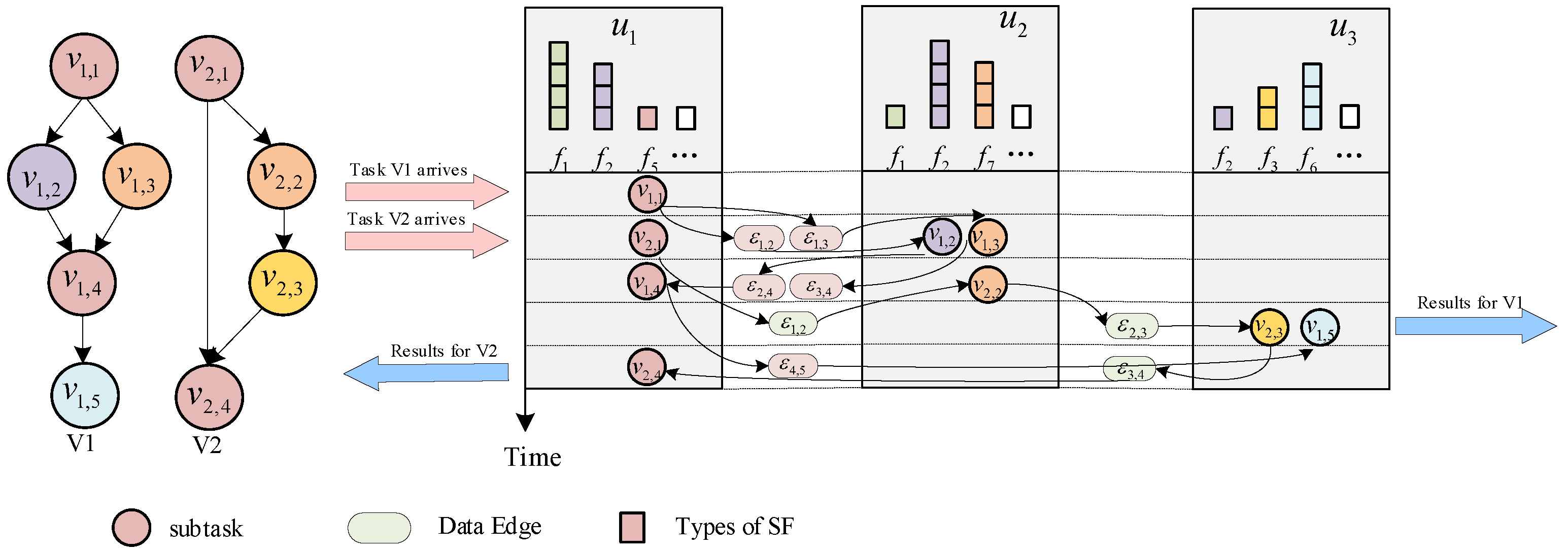
3.1.1. DAG Task Model

Consider a geographical area containing M mobile devices, which comprises a set of M independent tasks, represented by $\mathcal{V}=\{{\mathcal{V}}_1,{\mathcal{V}}_2,\dots ,{\mathcal{V}}_M\}$. The position of the m-th mobile device is assumed to be fixed, and is defined as $q_{G,m}=\{q_{G,m}^x,q_{G,m}^y,0\}$. Typically, each independent DAG task consists of multiple subtasks with data dependency. The structure of an independent task can be described as a DAG, denoted as $G=(V,\epsilon )$, where V is the set of subtasks, and $\epsilon$ is the set of edges connecting the subtasks. For example, the set of subtasks for the m-th task, i.e., ${\mathcal{V}}_m$, is denoted as ${\mathcal{V}}_m=\{v_{m,1},v_{m,2}\dots ,v_{m,i}\dots ,v_{m,{\alpha }_m}\}$, where ${\alpha }_m$ is the number of subtasks in the m-th DAG, and $v_{m,i}$ represents the i-th subtask in ${\mathcal{V}}_m$. If there is an edge from $v_{m,j}$ to $v_{m,i}$, i.e., ${\epsilon }_{(m,j),(m,i)}\in \epsilon$, the execution of $v_{m,i}$ depends on the result of $v_{m,j}$. $v_{m,j}$ is called the predecessor of $v_{m,i}$, while $v_{m,i}$ is the successor of $v_{m,j}$. A subtask can only be executed after all its predecessors are finished. In a DAG task, a subtask with no predecessors is called an entry subtask, and a task with no successor is called an exit subtask.

3.1.2. UAV Model

In total, R UAVs equipped with miniature base stations are dispatched to the area for providing communication and computation service. The set of UAVs is represented by $\mathcal{U}=\{u_1,u_2\dots ,u_r,\dots ,u_R\}$, where $u_r$ represents the r-th UAV. $u_r$’s position is defined as $q_{U,r}=\{q_{U,r}^x,q_{U,r}^y,H\}$. For simplicity, to ensure flight safety and communication quality, it is assumed that all UAVs are deployed at the same height, i.e., H. Here, H can be set to the lowest height that can avoid all obstacles within the service area. Defining a subtask offload decision variable $y_{v_{m,i}}^r$ as executing subtask $v_{m,i}$ on the r-th UAV, we have

$$\begin{array}{cc}\hfill & y_{v_{m,i}}^r\in \{0,1\},\forall m,i,r\hfill \end{array}$$

(1)

$y_{v_{m,i}}^r=1$ means that $v_{m,i}$ will be executed on the r-th UAV; otherwise, $y_{v_{m,i}}^r=0$. To ensure that each subtask can only be executed on one UAV, the following constraint should be fulfilled, i.e.,

$$\begin{array}{cc}\hfill & {\sum }_{r=1}^R{y}_{v_{m,i}}^r=1\hfill \end{array}$$

(2)

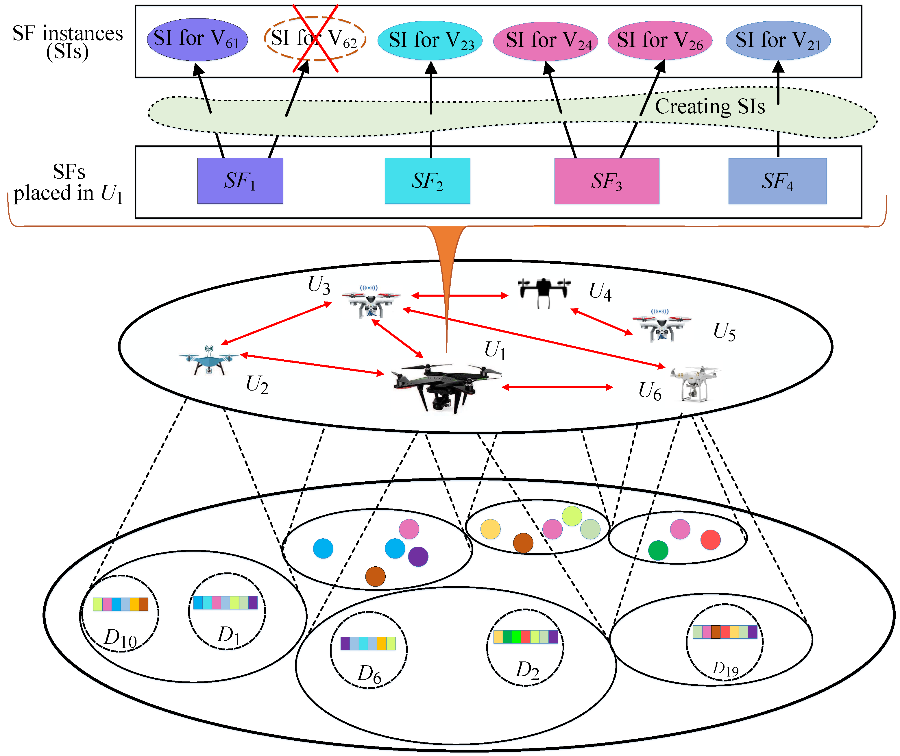
3.1.3. SF Deployment Model

An SF is the abstraction of the software and data for supporting the execution of a subtask [17]. The set of all SFs in the system is denoted as $\mathcal{F}=\{f_1,f_2,\dots ,f_Q\}$, where Q is the total number of SFs. Due to limited resources, each UAV can only deploy a subset of $\mathcal{F}$, denoted as ${\mathcal{F}}_r$. We require that there is at least one instance of an SF in the UAV network. Therefore, we have

$$\begin{array}{cc}\hfill & \mathcal{F}{}_1\cup \mathcal{F}{}_2\cup \dots \cup \mathcal{F}{}_R=\mathcal{F}\hfill \end{array}$$

(3)

where ${\mathcal{F}}_r$ is the set of SFs deployed on $u_r$. Assume that the total computation resources of the r-th UAV is $C_r$, and the number of CPU cycles allocated by the r-th UAV to subtask $v_{m,i}$ is denoted as $f_{v_{m,i}}^r$. Then, we have

$$\begin{array}{cc}\hfill & \sum _{s(m,i)\in F_r}{f}_{v_{m,i}}^r\le C_r\hfill \end{array}$$

(4)

Each subtask can be mapped to one SF in $\mathcal{F}$. Let $s(m,i)$ be the SF corresponding to the i-th subtask in the m-th DAG task. Therefore, $v_{m,i}$ can only be executed on a UAV that has deployed its corresponding SF. We have

$$\begin{array}{cc}\hfill & \forall v_{m,i}\in V,s(m,i)\in \mathcal{F}\hfill \end{array}$$

(5)

To describe the deployment of an SF on the UAV, define a decision variable $x_{s(m,i)}^r$ as

$$\begin{array}{cc}\hfill & x_{s(m,i)}^r\in \{0,1\},\forall m,i,r\hfill \end{array}$$

(6)

Here, $x_{s(m,i)}^r=1$ means $s(m,i)$ corresponding to $v_{m,i}$ will be deployed on the r-th UAV; $x_{s(m,i)}^r=0$ indicates that the r-th UAV will not deploy $s(m,i)$. There are constraints between the decision variable $x_{s(m,i)}^r$ and the parameter $y_{v_{m,i}}^r$, which are defined as follows:

$$\begin{array}{cc}\hfill & \left\{\begin{array}{c}\begin{array}{ccc}{x}_{s(m,i)}^r=1& if& y_{v_{m,i}}^r=1\end{array}\hfill \\ \begin{array}{ccc}{y}_{v_{m,i}}^r=0& if& x_{s(m,i)}^r=0\end{array}\hfill \end{array}\right.\hfill \end{array}$$

(7)

$y_{v_{{}_{m,i}}}^r=1$ means that $v_{m,i}$ is offloaded onto the r-th UAV. This can only be true when $x_{s(m,i)}^r=1$, i.e., $s(m,i)$ is deployed on the r-th UAV. In other words, $x_{s(m,i)}^r=1$ is a necessary but not sufficient condition for $y_{v_{{}_{m,i}}}^r=1$.

3.2. Task Execution Model

3.2.1. Communications Model

Three stages are required for processing a DAG task, i.e., task-uploading stage, task-computing stage, and results-returning stage. Following the common settings of previous works [18,19], this paper ignores the time consumed by the third stage since it is usually much less than that of the other two stages. For instance, for an image-recognition task, only the recognition results needs to be transmitted to the mobile device, and its occupied bandwidth can be neglected. During the mission calculation phase, multiple subtasks are offloaded simultaneously on each UAV. The time consumed by each subtask includes three parts, namely, the data transmission time, the waiting time, and the execution time as shown in Figure 2. During the mission upload phase, the data from the incoming subtasks of the DAG mission are transferred to the corresponding UAV. Therefore, the time of the mission upload phase is the data transfer time of the inbound subtask.

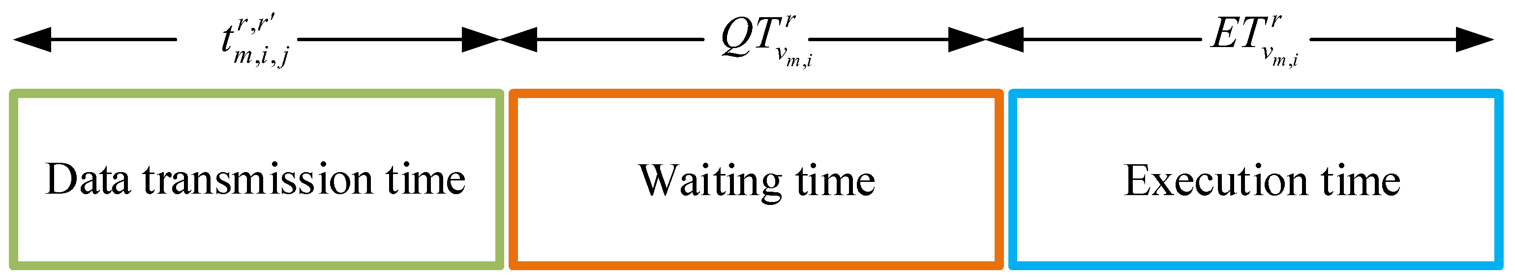
3.2.2. Data Transmission Time

A subtask’s data-transmission time refers to the time it takes for its input data to be transmitted from the device where the data are generated to its intended executing UAV. For an entry subtask, its input data are generated from the mobile device. For a non-entry subtask, its input data are generated from all its predecessor subtasks’ executing UAVs. Next, we describe them separately.

The data transmission time for the entry subtask. The m-th DAG task is generated from the m-th mobile device, and its entry subtask is represented as $v_{m,1}$. Define ${\gamma }_{v_{m,1}}$ as the UAV that executes $v_{m,1}$, then ${\gamma }_{v_{m,1}}\in \mathcal{U}$. Assume that it is offloaded onto the UAV ${\gamma }_{v_{m,1}}$. The probability that there is a line-of-sight (LoS) link between the m-th mobile device and the j-th UAV is

$$\begin{array}{cc}\hfill & P_{m,{\gamma }_{v_{m,1}}}^{Los}=\frac{1}{1+\psi .exp(-\beta ({\theta }_{m,{\gamma }_{v_{m,1}}}-\psi ))}\hfill \end{array}$$

(8)

The parameters depend on the communication probability and propagation environment. ${\theta }_{m,{\gamma }_{v_{m,1}}}$ refers to the angle of elevation between the mth device and the UAV, and is defined as

$$\begin{array}{cc}\hfill & {\theta }_{m,{\gamma }_{v_{m,1}}}=\frac{180}{\pi }\times {sin}^{-1}(\frac{H}{d_{m,{\gamma }_{v_{m,1}}}^{GU}})\hfill \end{array}$$

(9)

where H is the height of the UAV, and $d_{m,{\gamma }_{v_{m,1}}}^{GU}$ is the distance between the m-th mobile device and the UAV ${\gamma }_{v_{m,1}}$, defined as

$$\begin{array}{cc}\hfill & d_{m,{\gamma }_{v_{m,1}}}^{GU}=\Vert q_{U,{\gamma }_{v_{m,1}}}-q_{G,m}{\Vert }^2\hfill \end{array}$$

(10)

The transmission path loss between the m-th mobile device and the ${\gamma }_{v_{m,1}}$-th UAV is

$$\begin{array}{cc}\hfill & L_{m,{\gamma }_{v_{m,1}}}=\left\{{}_{{\eta }_2{(\frac{4\pi f{d}_{m,{\gamma }_{v_{m,1}}}^{GU}}{c})}^{\epsilon },Non-LosLink}^{{\eta }_1{(\frac{4\pi f{d}_{m,{\gamma }_{v_{m,1}}}^{GU}}{c})}^{\epsilon },LosLink}\right.\hfill \end{array}$$

(11)

where f is the carrier frequency; $\epsilon$ is the path loss exponent; ${\eta }_1$ and ${\eta }_2$ are the path loss coefficients for Los and Non-Los transmissions, respectively; and c is the speed of the light. The average transmission loss between the m-th mobile device and the ${\gamma }_{v_{m,1}}$-th UAV is

$$\begin{array}{cc}\hfill & {\stackrel{-}{L}}_{m,{\gamma }_{v_{m,1}}}=(P_{Los}^{m,{\gamma }_{v_{m,1}}}{\eta }_1+(1-P_{Los}^{m,{\gamma }_{v_{m,1}}}){\eta }_2){(\frac{4\pi f}{c}{d}_{m,{\gamma }_{v_{m,1}}}^{GU})}^{\epsilon }\hfill \end{array}$$

(12)

The received signal-to-interference-plus-noise ratio (SINR) at the UAV ${\gamma }_{v_{m,1}}$ from the m-th mobile device is

$$\begin{array}{c}\hfill {\gamma }_{m,{\gamma }_{v_{m,1}}}^{GU}=\frac{P_m^G}{(I_{m,{\gamma }_{v_{m,1}}}+{\sigma }^2){\stackrel{-}{L}}_{m,{\gamma }_{v_{m,1}}}}\end{array}$$

(13)

where $P_m^G$ is the transmission power of the m-th mobile device, $I_{m,{\gamma }_{v_{m,1}}}$ is the interference power of other electromagnetic spectrum devices, and ${\sigma }^2$ is the environmental noise power. In this case, the m-th mobile device will choose the UAV with the highest SINR value. The transmission rate from the m-th mobile device to the UAV ${\gamma }_{v_{m,1}}$ can be expressed as

$$\begin{array}{cc}\hfill & r_{m,{\gamma }_{v_{m,1}}}^{GU}=w_1{log}_2(1+{\gamma }_{m,{\gamma }_{v_{m,1}}}^{GU})\hfill \end{array}$$

(14)

where $w_1$ is the transmission bandwidth. The data transmission time for the entry task is

$$\begin{array}{cc}\hfill & t_{m,1}^{{\gamma }_{v_{m,1}}}=\frac{{\eta }_{v_{m,1}}}{r_{{}_{m,{\gamma }_{v_{m,1}}}}^{G,U}}\hfill \end{array}$$

(15)

where ${\eta }_{v_{m,1}}$ is the size of the input data bits for $v_{m,1}$.

The data transmission time of the non-entry subtask. Define $t_{m,i,j}^{r,r^{\prime }}$ as the data transmission time from subtask $v_{m,i}$ to its successor subtask $v_{m,j}$ in the m-th DAG task. Here, assume that $v_{m,i}$ and $v_{m,j}$ are executed on $u_r$ and $u_{r^{\prime }}$, respectively. The distance between $u_r$ and $u_{r^{\prime }}$ is

$$\begin{array}{cc}\hfill & d_{r{r}^{\prime }}^{UU}=\left|\right|q_{U,r^{\prime }}-q_{U,r}|{|}_2\hfill \end{array}$$

(16)

In the free space path loss model, the channel gain of the aerial link between $u_r$ and $u_{r^{\prime }}$ is ${\beta }_0{(d_{r{r}^{\prime }}^{UU})}^{-2}$, in which ${\beta }_0$ is the channel gain at distance $d=1m$. Therefore, the transmission rate between $u_r$ and $u_{r^{\prime }}$ is

$$\begin{array}{cc}\hfill & r_{r,r^{\prime }}^{UU}=w{log}_2(1+\frac{P_r^{UU}{\beta }_0}{{(d_{r{r}^{\prime }}^{UU})}^2{\sigma }^2})\hfill \end{array}$$

(17)

where w is the wireless transmission bandwidth of the wireless link between $u_r$ and $u_{r^{\prime }}$. $\frac{P_r^{UU}{\beta }^0}{{(d_{r{r}^{\prime }}^{UU})}^{-2}{\sigma }^2}\ge {\gamma }_0$ is the SINR received at $u_{r^{\prime }}$, and it is required to be larger than a predefined threshold ${\gamma }_0$. Let the amount of data bits transmitted from the $v_{m,i}$ to $v_{m,j}$ be $dat{a}_{i,j}^m$. The data transmission time will be

$$\begin{array}{cc}\hfill & t_{m,i,j}^{r,r^{\prime }}=\frac{dat{a}_{i,j}^m}{r_{r,r^{\prime }}^{UU}}\hfill \end{array}$$

(18)

When two subtasks are offloaded to the same UAV, i.e., $r=r^{\prime }$, note that $t_{m,i,j}^{r,r^{\prime }}=0$.

3.2.3. Waiting Time

The waiting time refers to the time duration between the arrival of a subtask’s input data and the start time of its execution. When multiple subtasks mapping to the same SF arrive at the UAV, a queue is built for each SF on the UAV. Each subtask has to wait at the queue until it is scheduled by the SF for execution. Define $Q{T}_{v_{m,i}}^r$ as the waiting time of $v_{m,i}$ on $u_r$, and it is determined by the queue length at the SF. Define $E{T}_k^r$ as the execution time of the k-th subtask in the queue. Assume that $v_{m,i}$’s position in the queue is ${\beta }^r$. Then, we have

$$\begin{array}{cc}\hfill & Q{T}_{v_{m,i}}^r=\sum _{k=1}^{{\beta }^r-1}E{T}_k^r\hfill \end{array}$$

(19)

3.2.4. Task Execution Time

$v_{m,i}$ can only be executed when all of its predecessor subtasks have completed and transmitted their results to $u_r$. The total amount of received data bits for executing $v_{m,i}$ is assumed to be ${\eta }_{v_{m,i}}$. The required number of CPU cycles for processing each bit is $c_{v_{m,i}}$. Let $f_{v_{m,i}}^r$ be the CPU frequency that $u_r$ assigns to execute $v_{m,i}$, and it can be obtained through a program analyzer. Define $E{T}_{v_{m,i}}^r$ as the task execution time of $v_{m,i}$, and it can be derived as

$$\begin{array}{cc}\hfill & E{T}_{v_{m,i}}^r=\frac{{\eta }_{v_{m,i}}{c}_{v_{m,i}}}{f_{v_{m,i}}^r}\hfill \end{array}$$

(20)

Let $S{T}_{v_{m,i}}^r$ be the earliest starting time of $v_{m,i}$. It is defined as

$$\begin{gathered} \begin{array}{cc}\hfill & S{T}_{v_{m,i}}^r=y_{v_{m,\mathrm{k}}}^{r^{″}}·y_{v_{m,i}}^r·x_{s(m,i)}^r·x_{s(m,k)}^{r^{″}}· \\ \underset{v_{m,\mathrm{k}}\in pre(v_{m,i})}{max}\{F{T}_{v_{m,k}}^{r^{″}}+t_{m,i,k}^{r,r^{″}}\}\hfill \end{array} \end{gathered}$$

(21)

where $F{T}_{v_{m,k}}^{r^{″}}$ is the completion time of its predecessor that is executed on $u_{r^{″}}$, $v_{m,k}\in pre(v_{m,i})$. Correspondingly, the completion time of $v_{m,i}$ on the $u_r$ is

$$\begin{array}{cc}\hfill & F{T}_{v_{m,i}}^r=S{T}_{v_{m,i}}^r+E{T}_{v_{m,i}}^r+Q{T}_{v_{m,i}}^r.\hfill \end{array}$$

(22)

The completion time of $v_{m,i}$ equals the sum of the execution time and waiting time of a task from the moment it begins execution. From the above equation, it can be inferred that the completion time of the last subtask of the m-th DAG task is $F{T}_{v_{m,{\alpha }_m}}^{{\gamma }_{v_{m,{\alpha }_m}}}$. Therefore, the response time of the m-th DAG task is

$$\begin{array}{cc}\hfill & R{T}_m=F{T}_{v_{m,{\alpha }_m}}^{{\gamma }_{v_{m,{\alpha }_m}}}-S{T}_{v_{m,1}}^{{\gamma }_{v_{m,1}}}\hfill \end{array}$$

(23)

3.3. Problem Statement

The main challenge for DAG task scheduling and SF deployment comes from the dependency among subtasks. Figure 3 shows an instance of the scenario, in which multiple DAG tasks need to be executed. In this circumstance, multiple queues are built on each UAV for its deployed SFs. This can lead to long waiting times due to the limited resources available for UAVs. Therefore, in the case of scheduling multiple DAG tasks, a parallel approach is adopted to solve the problem. In Figure 3, there are three UAVs, i.e., $u_1$, $u_2$, and $u_3$, and two DAG tasks, i.e., ${\mathcal{V}}_1$ and ${\mathcal{V}}_2$, whose structures are also shown. ${\mathcal{V}}_1$ includes five subtasks, and ${\mathcal{V}}_2$ contains four subtasks. The colored circles and squares represent the subtasks and data edges in the DAG tasks, respectively. $v_{11}$ in ${\mathcal{V}}_1$ is mapped to $f_5$, and it is scheduled onto $f_5$ on ${\mathrm{u}}_1$. Then, $v_{12}$ and $v_{13}$ are scheduled onto $f_2$ and $f_7$ deployed on ${\mathrm{u}}_2$. $v_{12}$ and $v_{13}$ are both the successor subtasks of $v_{11}$, and they can be executed in the same time. After the calculation is completed, the results are transmitted to $v_{14}$, and then to $v_{15}$. Finally, the execution results are output. ${\mathcal{V}}_2$’s entry subtask is $v_{21}$ and is also offloaded onto $u_1$, where $v_{11}$ is already located. Therefore, $v_{21}$ needs to wait for $v_{11}$ to be completed. Finally, when $f_5$ on $u_1$ is idle, and $v_{23}$ is completed, $v_{24}$ starts to execute, and finally outputs the execution result.

In this paper, the goal is to minimize the maximum completion time of all tasks:

$$\begin{array}{c}\hfill \begin{array}{c}\begin{array}{c}max\\ y_{v_{m,\mathrm{j}}}^{r^{\prime }},y_{v_{m,i}}^r,x_{s(m,i)}^r,x_{s(m,j)}^{r^{\prime }},q_r\end{array}\{F{T}_1,\dots ,F{T}_M\}\hfill \\ s.t.(1),(2),(4),(6),(7)\hfill \end{array}\end{array}$$

(24)

This is a non-linear programming problem with mixed 0-1 integers, and is a NP-hard problem. To solve this problem with low complexity, we propose an effective algorithm in the next section.

4. Algorithm Design

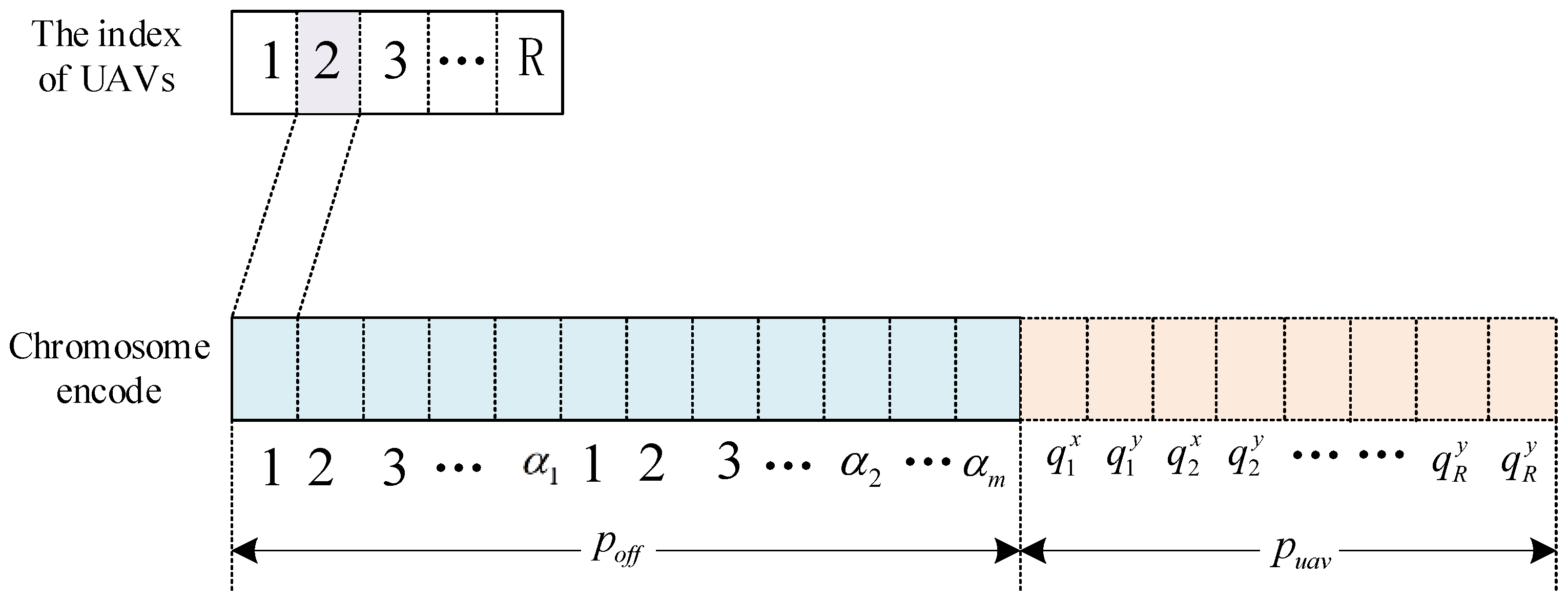
4.1. Chromosome Design

To apply the genetic algorithm for solving the problem in (24), we first need to map the solution to this problem as an individual or chromosome. To be specific, each chromosome contains two parts: the first part is adopted to reflect the subtask offloading decision, expressed in $p_{off}$; the second part is the positions of the UAVs, expressed in $p_{uav}$ as shown in Figure 4. The offloading decision of each subtask is coded as an integer between 1 and R, which represents the index of the UAV executing this subtask. For example, if $v_{11}$ is offloaded on $u_2$, the gene coding for $v_{11}$ is 2. The latter part of the chromosome is encoded as the positions of R UAVs. In total, each chromosome has $D={\displaystyle \sum _{m=1}^M}{\displaystyle \sum _{i=1}^{{\alpha }_m}}{v}_{m,i}+2R$ genes. For each individual, its fitness value is set to be the reciprocal of its maximum completion time calculated using (24). This can ensure that the solution that can achieve a lower maximum completion time will obtain a higher fitness value.

4.2. Algorithm Design

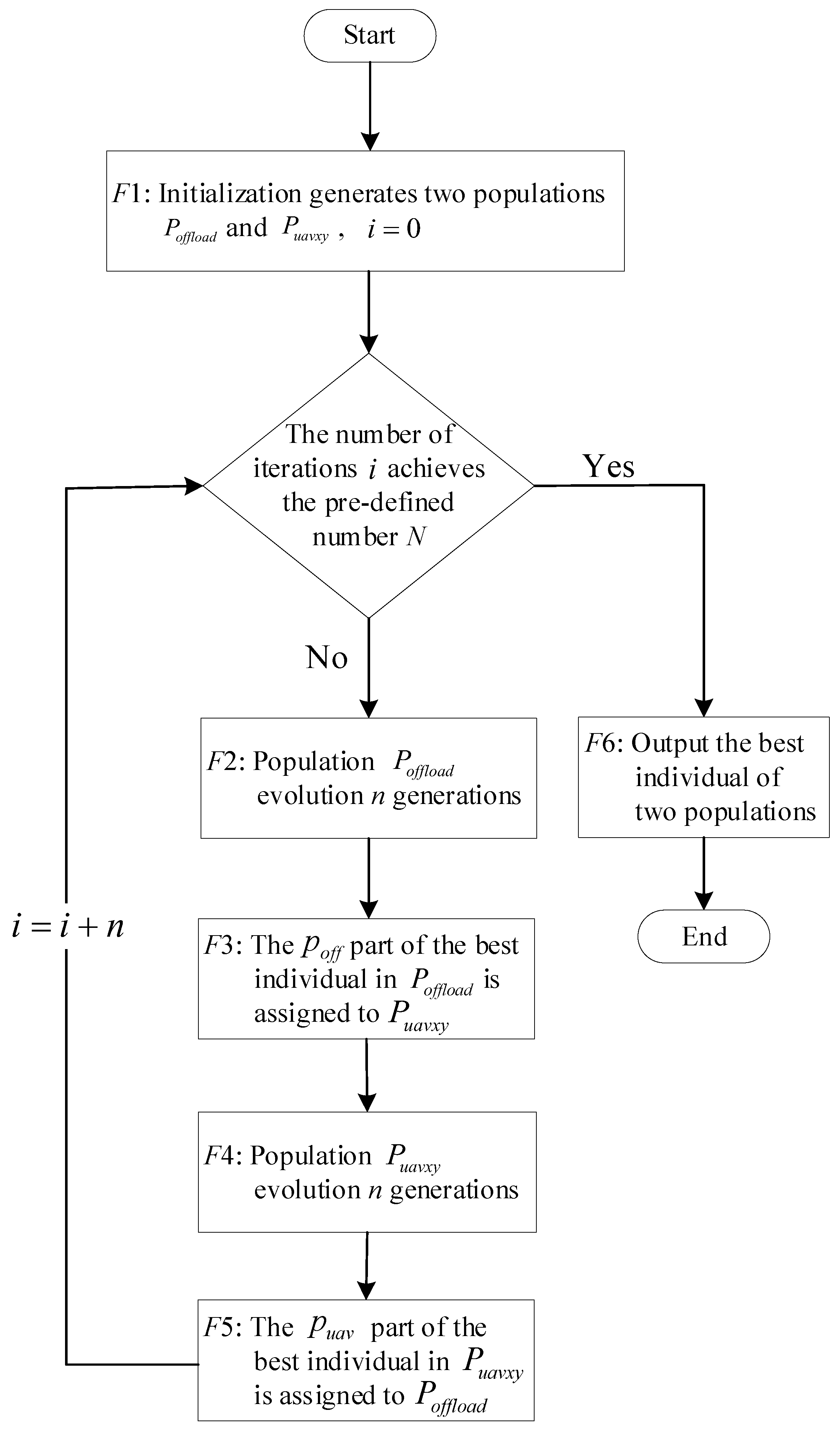
4.2.1. Overall Working Flow

To accelerate the convergence of genetic algorithm’s iteration process, we propose the GA-based joint deployment and scheduling (GA-JoDeS) algorithm, and generate two populations, one for subtask offloading decision making, i.e., $P_{offload}$, and the other for the UAV position determination, i.e., $P_{uavxy}$. Each population includes G number of individuals with size D. The overall iteration process is shown in Figure 5. At first, both $P_{offload}$ and $P_{uavxy}$ are randomly initialized, and are optimized in an iterative manner. To be specific, each individual in $P_{offload}$ only interacts, including selection, crossover and mutation with individuals within $P_{offload}$. Moreover, during each operation, only genes in the first part, i.e., $p_{off}$, are changed, and those genes in $p_{uav}$ remain the same. This is also true for those individuals in $P_{uavxy}$. This means individuals in $P_{uavxy}$ can only be operated with other individuals in $P_{uavxy}$, and genes in $p_{off}$ remain the same during this process. The individuals in $P_{offload}$ first evolve for n rounds to find the best offloading decision for a fixed $p_{uav}$, which is shown in process $F2$ of Figure 5, and its pseudo code is described in Algorithm 1. Then, as shown in process $F3$ of Figure 5, $p_{off}$ of the best individual in $P_{offload}$ is assigned to the first part of all the individuals in $P_{uavxy}$. Then, individuals in $P_{uavxy}$ first evolve for n rounds to find the best UAVs’ position determination for a fixed $p_{off}$, which is shown in process $F4$ of Figure 5, and its pseudo code is described in Algorithm 1 too. Afterwards, as shown in process $F5$ of Figure 5, $p_{uav}$ of the best individual in $P_{uavxy}$ is assigned to the second part of all the individuals in $P_{offload}$. In this way, both $P_{offload}$ and $P_{uavxy}$ can evolve with iterations until the number of iterations achieves the pre-defined number N.

4.2.2. Population Evolve Process

As we can see in Figure 5, $F1$, $F2$ and $F4$ are both populations’ evolution processes. Algorithm 1 provides pseudo code for the evolution of n generation. The inputs include the population size G, crossing probability $pc$, mutation probability $pm$, and the population P. The output of Algorithm 1 is the next generation of the population $pop$. Evolutionary processes include selection, crossover, mutation, etc. The algorithm starts by initializing G number of individuals using random sampling, which costs the time complexity $o(G)$. In the process of chromosome selection, Steps 2–8 select superior individuals and eliminate inferior ones in the population. Here, G number of individuals are selected. After selection, Steps 9–17 select two individuals for crossover; using a two-point crossover approach, the cases of $P_{offload}$ and $P_{uavxy}$ are considered separately. After the crossover is completed, Steps 18–31 consider the cases of $P_{offload}$ and $P_{uavxy}$, respectively, and select the individuals and genes for mutation by $pm$. In crossover and mutation operations, the time complexity is related to the total number of iterations and the dimension of chromosome genes. Step 32 obtains the evolved population $pop$. The time complexity of the proposed Algorithm 1 is $o(n.G.D)$, where G is the number of individuals, D is the dimension of the population individual and n is the maximum evolution generation.

Algorithm 1 Population evolution in GA-JoDeS algorithm.

Input: population P, population size G, crossing probability $pc$, mutation probability $pm$, evolved generations n

Output: evolved population $pop$.   1: for $i\in (1,2\dots ,n)$ do   2:     Evaluate all fitness $fi{t}_P$ of P, retain the individual with the largest fitness value, $pop\Leftarrow P_{best}$.   3:     Compute min fitness $Z_{min}={min}_{j\in (1,G)}fi{t}_{P_j}$.   4:     The sum of fitness $total=0$.   5:     Fitness for each individual minus minimum fitness $fi{t}_P\leftarrow fi{t}_P-Z_{min}$.   6:     The sum of fitness $total={\displaystyle \sum _{j=1}^G}fi{t}_{P_j}$.   7:     The proportion of fitness for each individual $p{s}_P=fi{t}_P/total$.   8:     Select $G-1$ individuals by roulette wheel algorithm,     $pop\Leftarrow \{P_{k1},P_{k2},\dots P_{kn},\dots ,P_{k\left(G-1\right)}\},kn\in (1,G-1)$.   9:    for $i=1$ to G do 10:        According to $pc$ select two individuals $po{p}_i$ and $po{p}_j$. 11:        Two intersections p and q are randomly selected of $po{p}_j$. 12:        if $P==P_{offload}$ then 13:           Cross $po{p}_i$ and $po{p}_j$, the new $po{p}_i$ which is composed of three parts:      $\{po{p}_i^0,po{p}_i^{p-1}\}$, $\{po{p}_j^p,po{p}_j^q\}$, $\{po{p}_i^{q+1},po{p}_i^{D-2R}\}$. 14:        else 15:           Cross $po{p}_i$ and $po{p}_j$, the new $po{p}_i$ which is composed of three parts:      $\{po{p}_i^{D-2R+1},po{p}_i^{p-1}\}$, $\{po{p}_j^p,po{p}_j^q\}$, $\{po{p}_i^{q+1},po{p}_i^D\}$. 16:        end if 17:    end for 18:    for $i=1$ to G do 19:        According to $pm$ select a individual $po{p}_i$ for mutation. 20:        if $P==P_{offload}$ then 21:            for $j=1$ to $D-2R$ do 22:                According to $pm$ select a point for mutation. 23:                The point’s corresponding subtask reselect UAV randomly. 24:            end for 25:        else 26:             for $j=D-2R+1$ to D do 27:                 According to $pm$ select a point for mutation. 28:                 the point’s corresponding UAV reassign a position. 29:              end for 30:         end if 31:     end for 32: end for 33: Return the evolved population $pop$.

Initialization. As described above, both $P_{offload}$ and $P_{uavxy}$ are randomly initialized. Firstly, initializing $p_{off}$ of the $P_{offload}$ individuals, each subtask randomly select a UAV in $U_{set}$, which is a set of UAVs that have been deployed the subtask’s corresponding SF or whose remaining resource is greater than the resource required by the subtask. Secondly, initializing $p_{uav}$ of the $P_{uavxy}$ individuals, each UAV randomly generates a position for which the value is an integer in the range. Thirdly, initialize $p_{uav}$ of the $P_{offload}$ individuals by assigning the $p_{uav}$ of the first individual in $P_{uavxy}$ to the second part of all individuals in $P_{offload}$. Lastly, initialize $p_{off}$ of $P_{uavxy}$’s individuals by assigning the $p_{off}$ of the first individual in $P_{offload}$ to the first part of all individuals in $P_{uavxy}$.

Selection. Before selecting individuals for evolved population $pop$, the fitness of all individuals is calculated. $pop$ will firstly retain the individual with the largest fitness value. In order to increase the gap in the probability that an individual is selected before, the fitness value of each individual is subtracted from the minimum value of all fitness values. Then, by the roulette wheel algorithm, a select G number of individuals are retained to $pop$.

Crossover. Two individuals, for instance, $p_i$ and $p_j$, for crossover are based on the crossing probability $pc$. In $P_{offload}$ (or $P_{uavxy}$), only the genes in $p_{off}$ (or $p_{uav}$) contained in $p_i$ and $p_j$ will engage in the crossover process, while $p_{uav}$ ($p_{off}$) in $p_i$ and $p_j$ is not affected. Two intersections are randomly generated for crossover, and the genes in $p_j$ between the two intersections are assigned to $p_i$. After the crossover operation, only $p_i$ is changed.

Mutation. Mutation can prevent the algorithm from getting stuck in a local optimum, and the mutation probability is controlled by parameter $pm$. Based on $pm$, an individual $p_i$ is randomly selected for mutation. If $p_i$ is chosen from $P_{offload}$, all genes in $p_{off}$ of individual $p_i$ will mutate with probability $pm$, i.e., the mutated subtask re-selects a UAV for offloading. If $p_i$ is chosen from $P_{uavxy}$, all genes in $p_{uav}$ of individual $p_i$ will mutate with probability $pm$, i.e., the mutated UAV reassigns a new position, which is adjacent to the UAV current position.

Note that in the initialization, crossover, and mutation process, if a subtask cannot select an eligible UAV to offload, it will select a UAV randomly, release all subtasks on the selected UAV and offload the subtask to the UAV; other released subtasks re-select UAVs. The above process ensures that each subtask has a UAV to offload.

Finally, the optimal individual is selected to determine the subtasks’ offloading decision and the positions of the UAVs. The SF deployment results are determined based on the subtask offloading decision. In other words, if the subtask is offloaded on that UAV, then the SF corresponding to the subtask must be placed on the UAV.

5. Simulation and Results Analysis

5.1. Experimental Setup

Consider a service scenario with 10 UAVs that are deployed in a 500 m × 500 m area. Each UAV offload corresponding subtask has a height of 100 m, and the average resource of the UAVs is abstracted to one dimension and has an average resource range of 20 to 80 units. The DAG of each arrived task contains 5, 6, or 7 sub-tasks, and the weights on the edge between two subtasks fall between 0.6 Mb and 2 Mb. There are 20 different SFs in total, and they vary from 2 to 8. The main parameter settings are included in

Table 3. Parameter settings.

Simulation Parameters	Value
$sf$	20
R	10
$x^r$	[1, 500] m
$y^r$	[1, 500] m
H	100 m
$\psi$	11.95
$\beta$	0.14
$\epsilon$	2
${\eta }_1$	3
${\eta }_2$	10
f	2 GHz
$\sigma 2$	${10}^{-6}$
$Iij$	${10}^{-6}$
$w_1$	200 MHz
$P_j^{UG}$	${10}^5$ w
w	2 MHz
${\beta }_0$	$1.4\times {10}^{-3}$
$pc$	0.8
$pm$	0.2
$f_{v_{m,i}}^r$	[2, 8]
N	600

.

To evaluate the performance of the GA-JoDeS algorithm, three algorithms are chosen as comparison benchmarks:

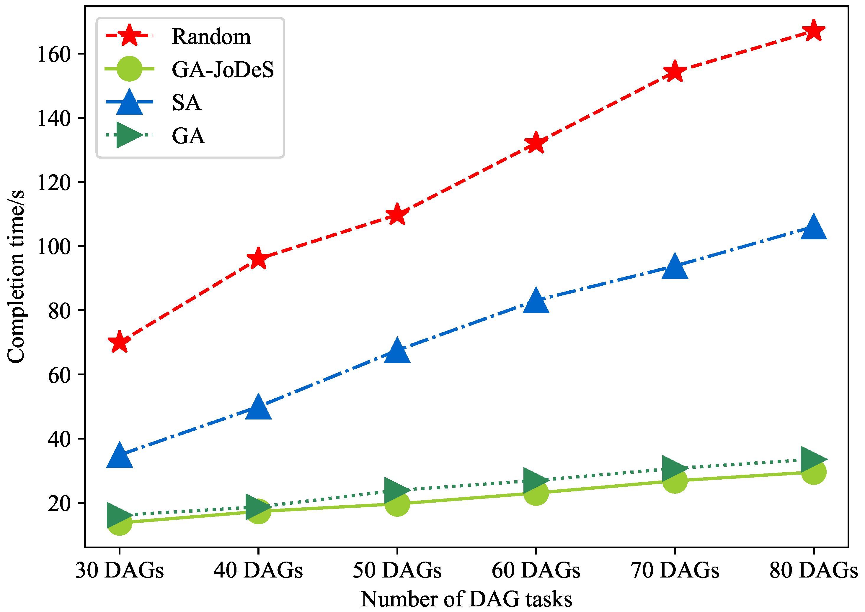
• Random algorithm: The subtasks randomly select UAVs to offload, and the positions of UAVs are also randomly generated within the range.
• Genetic algorithm (GA): The chromosome coding part is the same as the GA-JoDeS. G number of individuals is generated in the population. The opposite of the total task completion time of an individual is set as the fitness value. The roulette wheel algorithm is utilized to select good individuals to form a new population next by single-point crossover and mutation between individuals. N generations are generated to obtain the best individual.
• Simulated annealing (SA) algorithm: First, an initial solution is generated based on the task offloading schedule and the positions of the UAVs; then the maximum completion time of the solution is calculated. Afterwards, the initial temperature, end temperature, and temperature drop factor in the algorithm are determined. The initial solution is randomly changed several times, and the difference between the changed objective function value and the initial value is recorded. The metropolis criterion is utilized to determine whether the change would be accepted. If the new solution is accepted as the current solution, a new temperature is set according to the temperature drop factor. The above steps are repeated until the temperature is lower than the end temperature.

5.2. Results and Analysis

This experiment was run in a Python environment with a processor of the 12th i9-12900KF. The average running time is 10 min for the algorithm to achieve merit convergence.To ensure the accuracy of each experimental result, at least 20 simulations were conducted for different initial values and algorithms, and the average value was taken as the experiment result and recorded.

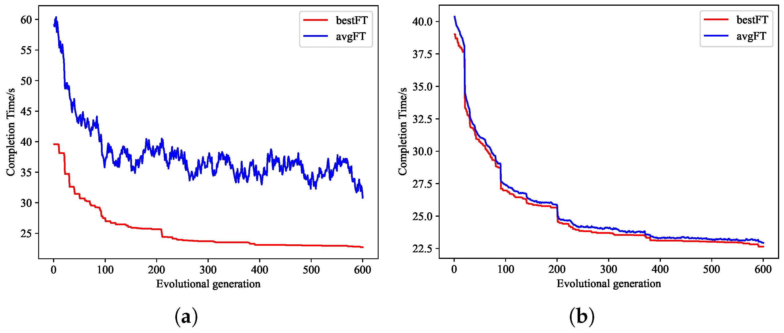
5.2.1. The Convergence of the GA-JoDeS

Figure 6 shows the completion time of GA-JoDeS with the increase in the evolutional generation when there are 60 DAG tasks, and the average resource of the UAVs is 40 units. One can see that GA-JoDeS converges quickly to a stable state. According to the GA-JoDeS, the alternate optimization method is used to optimize $p_{off}$ (as shown in Figure 6a) and $p_{uav}$ (as shown in Figure 6b), separately. The “avgFT” represents the average completion time of an individual in a certain generation, and the “bestFT” represents the best completion time of an individual in a certain generation. It can be seen that as the number of evolution generations increases, the “bestFT” gradually decreases in each generation, and “avgFT” also shows a downward trend. After several repeated experiments, we found that when the evolution generation is set to 600, the “avgFT” and the “bestFT” gradually approach each other, and the graph tends to be stable, proving that GA-JoDeS has good convergence ability.

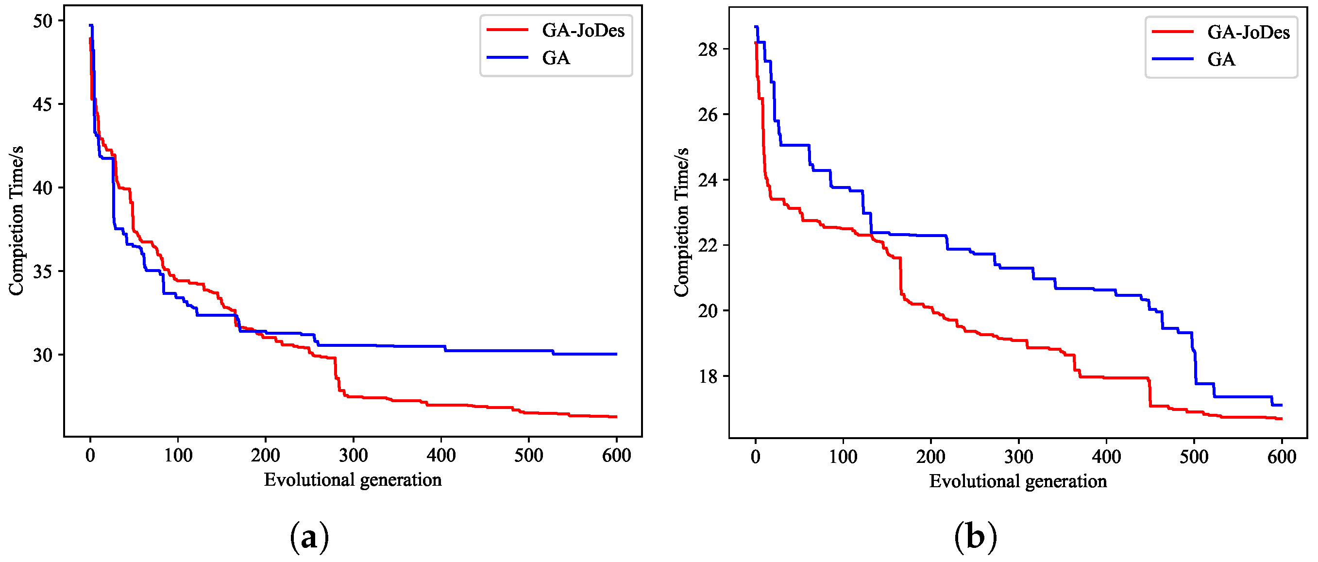
5.2.2. The Comparison of Rate of Convergence of GA-JoDeS and GA

Figure 7a,b show the comparison of the rate of convergence of GA-JoDeS and GA when the number of DAG tasks is set to 70 and the resource is set to 40 units, and the number of DAG tasks is set to 50 and the resource is set to 60 units, respectively. The red and blue curves represent the GA-JoDeS and GA algorithms, respectively. As shown in Figure 7, the completion time of the subtasks decreases with the increase in the evolution generation. Furthermore, during the evolution process, we can observe that the completion time of GA-JoDeS is always less than GA, and the descent speed is greater than GA. The phenomenon shows that GA-JoDeS not only has a faster rate of convergence than GA but also has a better final convergence result than GA.

5.2.3. Results Analysis with Different Number of Tasks

Figure 8 shows the comparison of the completion time of different algorithms with different numbers of DAG tasks. The number of DAG tasks is set to be 30, 40, 50, 60, 70, and 80, respectively, while the average resource of the UAVs is 40 units. The evolutionary generation, i.e., N of GA-JoDeS and GA, is 600. The population size is 80. In the SA algorithm, the initial and end temperatures are 100 and 0.1, respectively; the temperature drop factor is 0.99.

From Figure 8, one can see that as the number of DAG tasks increases, the completion time of the four algorithms gradually increases. This is due to the fact that we offload all subtasks in a parallel model since the resources of UAVs become tense, making it difficult for subtasks to find a suitable time slot, increasing the queuing time and the overall latency when the number of DAG tasks increases. The GA-JoDeS algorithm significantly outperforms the other three algorithms in the completion time of tasks, especially when the number of DAG tasks is large. This is mainly because the resource of the UAVs for subtask offloading is relatively sufficient. When the number of DAG tasks is smaller, subtasks can easily find suitable UAVs for offloading, so the advantages of GA-JoDeS are not obvious. However, when the number of DAG tasks increases, the results obtained by GA-JoDeS are significantly better than that of other algorithms, which also proves the superiority of the GA-JoDeS algorithm.

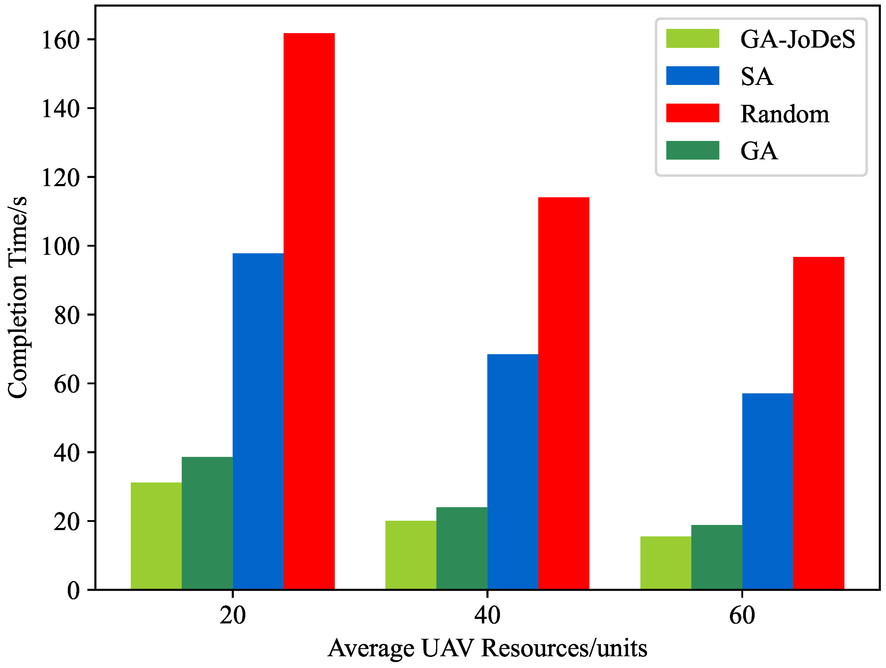
5.2.4. Results Analysis with Different Resources

Figure 9 shows the comparison of the completion time of different algorithms with different resources. The number of DAG tasks is 50, the population size is 80, and the average resource of UAVs is 20, 40, and 60 units, respectively. From the Figure 9, we can see that the GA-JoDeS algorithm’s tasks completion time is remarkably lower than that of the other three algorithms. When the UAVs’ resources are fewer, the task completion time gradually increases. Therefore, the following conclusions can be drawn from the results. When the UAVs resources are sufficient, on the one hand, subtasks can be offloaded flexibly between multiple UAVs and more suitable time slots can be found for execution, thereby shortening the overall latency and improving the system performance; on the other hand, as the UAVs resources increase, subtasks can easily find UAVs that meet the conditions for offloading.

5.2.5. The Distribution of SFs

Table 4. The deployment of SFs on UAVs.

Average Resource of a UAV	20	40
SFs deployed on $U_0$	$f_2,f_7,f_8,f_{15},f_{17},f_{19}$	$f_2,f_3,f_4,f_5,f_6,f_7,f_{10},f_{11},f_{14},f_{15},f_{19}$
SFs deployed on $U_1$	$f_3,f_4,f_5,f_{11},f_{13},f_{19}$	$f_1,f_3,f_4,f_5,f_6,f_8,f_{13},f_{14},f_{15},f_{16},f_{19}$
SFs deployed on $U_2$	$f_3,f_5,f_6,f_{11},f_{14},f_{15}$	$f_3,f_4,f_5,f_6,f_9,f_{10},f_{11},f_{14},f_{15},f_{17},f_{19}$
SFs deployed on $U_3$	$f_{10},f_4,f_{13},f_7$	$f_1,f_2,f_3,f_5,f_7,f_9,f_{11},f_{12},f_{13},f_{15},f_{18},f_{19}$
SFs deployed on $U_4$	$f_7,f_9,f_{11},f_{12},f_{15},f_{16},f_{19}$	$f_1,f_2,f_3,f_5,f_6,f_7,f_9,f_{11},f_{12},f_{15},f_{16},f_{18}$
SFs deployed on $U_5$	$f_2,f_7,f_9,f_{16},f_{18},f_{19}$	$f_1,f_4,f_6,f_7,f_8,f_{10},f_{11},f_{12},f_{17},f_{19}$
SFs deployed on $U_6$	$f_1,f_9,f_{10},f_{11},f_{17}$	$f_2,f_3,f_4,f_5,f_7,f_{11},f_{14},f_{15},f_{16},f_{17},f_{18},f_{19}$
SFs deployed on $U_7$	$f_1,f_4,f_8,f_9,f_{15},f_{18}$	$f_1,f_2,f_4,f_6,f_7,f_{10},f_{11},f_{12},f_{13},f_{19}$
SFs deployed on $U_8$	$f_1,f_4,f_{11},f_{13},f_{14},f_{15}$	$f_2,f_3,f_5,f_6,f_8,f_9,f_{11},f_{13},f_{16},f_{18}$
SFs deployed on $U_9$	$f_3,f_6,f_9,f_{13},f_{16}$	$f_1,f_3,f_7,f_8,f_{11},f_{12},f_{14},f_{15},f_{16},f_{17},f_{18}$
The maximum task completion time	63.27 s	18.77 s

illustrates the distribution of SFs types and completion time among ten UAVs with 80 DAG tasks when resources are 20 units and 40 units, respectively. The SFs deployment on the UAVs are determined by the subtasks offloading decision. As shown in Table 4, when the UAVs resources are 20 units, there are relatively few UAVs with SFs types corresponding to subtasks, resulting in longer queue times for subtasks during offloading, and longer total task completion time compared to when resources are sufficient.

5.2.6. The Positions of UAVs

Figure 10 and Figure 11 show the derived positions of UAVs by the GA-JoDeS algorithm in different scenarios. At first, the UAVs positions are randomly determined. Through optimization, the optimal individual is eventually obtained, and the positions of the UAVs are shown in Figure 10. It can be seen that the positions of ten UAVs are gradually converged. During the calculation process, the maximum task completion time consists of the transmission time and the subtasks execution time, and the data transmission time between UAVs accounts for a large proportion. Therefore, during the optimization process, to reduce the data transmission time, the positions of the UAVs gradually approach each other. The experimental results also confirm this phenomenon.

Figure 11 shows the UAVs positions when 50 DAG tasks are deployed within a small area between 350 m and 400 m. The entry subtask of each DAG task has a large data volume. As shown in Figure 11, UAVs will move to the deployed area of DAG tasks. When the data volume of the entry subtasks is large, the transmission time between the entry subtask and the UAV account for a relatively large proportion of the total completion time. Therefore, the UAVs gradually approached the location of the DAG tasks. This demonstrates that when the location of the DAG tasks is known, this algorithm can be used to determine the best locations for the UAVs.

6. Conclusions

In this paper, we consider the offloading of DAG tasks in UAV-empowered edge computing, and minimize the task completion time by combining the UAVs positions, SFs deployment and DAG tasks scheduling. According to the above, we build an 0–1 optimization problem. Then, an algorithm named GA-JoDeS is put forward to find the optimal solution of the problem. To evaluate the performance of the GA-JoDeS algorithm, three algorithms are chosen as comparison benchmarks. Results show that the GA-JoDeS algorithm always outperforms the other three algorithms in its maximum completion time of DAG tasks. The same observations can be made with different parameter settings, such as the number of DAG tasks, the resource occupied by a UAV, etc.

We will investigate the scenario in which mobile devices or DAG tasks can move dynamically in the deployment area in the future.

References

1. Ra, M.R.; Sheth, A.; Mummert, L.B.; Pillai, P.; Govindan, R. Odessa: Enabling Interactive Perception Applications on Mobile Devices. In Proceedings of the International Conference on Mobile Systems, Washington, DC, USA, 28 June–1 July 2011. [Google Scholar]
2. Wei, X.; Liu, J.; Wang, Y.; Tang, C.; Hu, Y. Wireless edge caching based on content similarity in dynamic environments. J. Syst. Archit. 2021, 115, 102000. [Google Scholar] [CrossRef]
3. Wei, X.; Tang, C.; Fan, J.; Subramaniam, S. Joint optimization of energy consumption and delay in cloud-to-thing continuum. IEEE Internet Things J. 2019, 6, 2325–2337. [Google Scholar] [CrossRef]
4. Hu, Q.; Cai, Y.; Yu, G.; Qin, Z.; Zhao, M.; Li, G.Y. Joint offloading and trajectory design for UAV-enabled mobile edge computing systems. IEEE Internet Things J. 2018, 6, 1879–1892. [Google Scholar] [CrossRef]
5. Zhao, N.; Cheng, F.; Yu, F.R.; Tang, J.; Chen, Y.; Gui, G.; Sari, H. Caching UAV assisted secure transmission in hyper-dense networks based on interference alignment. IEEE Trans. Commun. 2018, 66, 2281–2294. [Google Scholar] [CrossRef] [Green Version]
6. Yang, Z.; Pan, C.; Wang, K.; Shikh-Bahaei, M. Energy efficient resource allocation in UAV-enabled mobile edge computing networks. IEEE Trans. Wirel. Commun. 2019, 18, 4576–4589. [Google Scholar] [CrossRef]
7. Yu, Z.; Gong, Y.; Gong, S.; Guo, Y. Joint task offloading and resource allocation in UAV-enabled mobile edge computing. IEEE Internet Things J. 2020, 7, 3147–3159. [Google Scholar] [CrossRef]
8. Ren, Y.; Xie, Z.; Ding, Z.; Sun, X.; Xia, J.; Tian, Y. Computation offloading game in multiple unmanned aerial vehicle-enabled mobile edge computing networks. IET Commun. 2021, 15, 1392–1401. [Google Scholar] [CrossRef]
9. Ei, N.N.; Kang, S.W.; Alsenwi, M.; Tun, Y.K.; Hong, C.S. Multi-UAV-assisted MEC system: Joint association and resource management framework. In Proceedings of the 2021 International Conference on Information Networking (ICOIN), Jeju Island, Republic of Korea, 13–16 January 2021; pp. 213–218. [Google Scholar]
10. Mach, P.; Becvar, Z. Mobile edge computing: A survey on architecture and computation offloading. IEEE Commun. Surv. Tutorials 2017, 19, 1628–1656. [Google Scholar] [CrossRef] [Green Version]
11. Wei, X.; Cai, L.; Wei, N.; Zou, P.; Zhang, J.; Subramaniam, S. Joint UAV Trajectory Planning, DAG Task Scheduling, and Service Function Deployment based on DRL in UAV-empowered Edge Computing. IEEE Internet Things J. 2023, 1–13. [Google Scholar] [CrossRef]
12. Li, D.C.; Chen, B.H.; Tseng, C.W.; Chou, L.D. A novel genetic service function deployment management platform for edge computing. Mob. Inf. Syst. 2020, 2020, 1–22. [Google Scholar] [CrossRef]
13. Cai, L.; Wei, X.; Xing, C.; Zou, X.; Zhang, G.; Wang, X. Failure-resilient DAG task scheduling in edge computing. Comput. Netw. 2021, 198, 108361. [Google Scholar] [CrossRef]
14. Zhan, C.; Hu, H.; Sui, X.; Liu, Z.; Niyato, D. Completion time and energy optimization in the UAV-enabled mobile-edge computing system. IEEE Internet Things J. 2020, 7, 7808–7822. [Google Scholar] [CrossRef]
15. Zhang, T.; Xu, Y.; Loo, J.; Yang, D.; Xiao, L. Joint computation and communication design for UAV-assisted mobile edge computing in IoT. IEEE Trans. Ind. Inform. 2019, 16, 5505–5516. [Google Scholar] [CrossRef] [Green Version]
16. Xu, Y.; Zhang, T.; Yang, D.; Xiao, L. UAV-assisted relaying and MEC networks: Resource allocation and 3D deployment. In Proceedings of the 2021 IEEE International Conference on Communications Workshops (ICC Workshops), Montreal, QC, Canada, 14–23 June 2021; pp. 1–6. [Google Scholar]
17. Gao, Y.; Guan, H.; Qi, Z.; Yang, H.; Liang, L. A multi-objective ant colony system algorithm for virtual machine placement in cloud computing. J. Comput. Syst. Sci. 2013, 79, 1230–1242. [Google Scholar] [CrossRef]
18. Kao, Y.H.; Krishnamachari, B.; Ra, M.R.; Fan, B. Hermes: Latency optimal task assignment for resource-constrained mobile computing. In Proceedings of the 2015 IEEE Conference on Computer Communications (INFOCOM), Kowloon, Hong Kong, 26 April–1 May 2015. [Google Scholar]
19. Zhang, W.; Wen, Y.; Wu, D.O. Collaborative Task Execution in Mobile Cloud Computing Under a Stochastic Wireless Channel. Wirel. Commun. IEEE Trans. 2015, 14, 81–93. [Google Scholar] [CrossRef]
Figure 1. The multi-UAV-empowered edge-computing scenario. Multiple UAVs compose an aerial network, and they collaborate with each other to provide services to mobile devices on the ground. Each mobile device has a DAG task to be offloaded. Each DAG task consists of multiple subtasks with dependencies, and the execution of each subtask requires a corresponding SF, which contains the necessary software module and data for executing the subtask. Due to the limited available resource on each UAV, it can only support the parallel execution of a few SFs. Note that different subtasks in the same DAG task can be executed on different UAVs. This will lead to data transmission among UAVs.
Drones 07 00443 g001
Figure 2. Subtask offload process.
Drones 07 00443 g002
Figure 3. Task scheduling instance.
Drones 07 00443 g003
Figure 4. Chromosome encoding.
Drones 07 00443 g004
Figure 5. GA-based joint deployment and scheduling (GA-JoDeS) algorithmic processes.
Drones 07 00443 g005
Figure 6. Comparison graph of average completion time and optimal completion time under different evolutionary generations. (a) Subtask offloading decision; (b) the UAVs positions.
Drones 07 00443 g006
Figure 7. The comparison of rate of convergence of GA-JoDeS and GA. (a) The number of DAG tasks is set to 70 and the resource is set to 40 units; (b) the number of DAG tasks is set to 50 and the resource is set to 60 units.
Drones 07 00443 g007
Figure 8. The completion time of different number of DAGs under different algorithms.
Drones 07 00443 g008
Figure 9. The completion time of different UAVs resources under different algorithms.
Drones 07 00443 g009
Figure 10. DAG tasks distributed randomly.
Drones 07 00443 g010
Figure 11. DAG tasks distributed within a fixed range.
Drones 07 00443 g011