Figure 1.
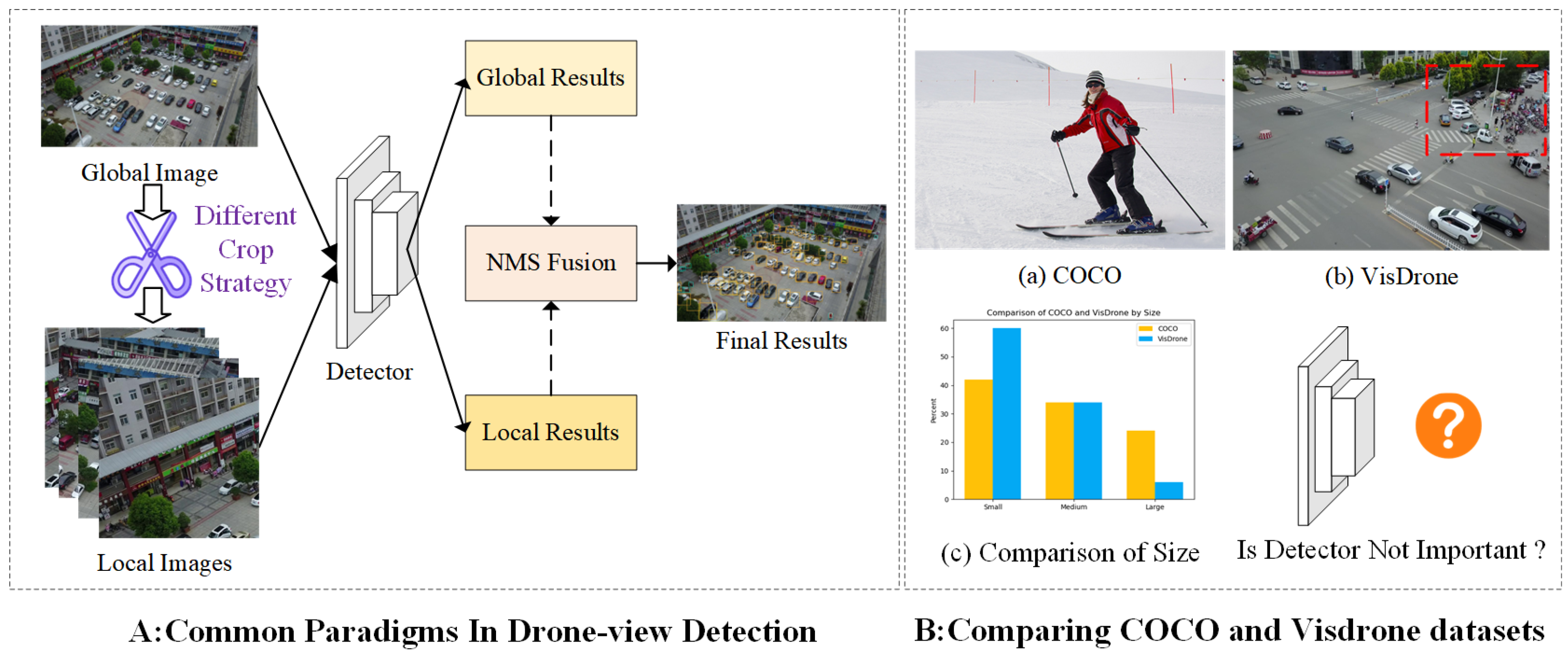
Most current paradigms treat drone-view object detection as a conventional object detection task, where different cropping strategies are applied first and then passed through unmodified detectors. This approach neglects the unique characteristics of aerial scenes, such as intense scale variations and a large number of small objects.
Figure 1.
Most current paradigms treat drone-view object detection as a conventional object detection task, where different cropping strategies are applied first and then passed through unmodified detectors. This approach neglects the unique characteristics of aerial scenes, such as intense scale variations and a large number of small objects.
Figure 2.
DroneNet consists of three components: FIEM, SCFPN, and CRLA. FIEM is utilized to enhance the features of the backbone network, SCFPN is employed to fuse different feature layers, particularly to leverage information from feature layers related to small objects, while CRLA is responsible for selecting high-quality positive samples of small objects to be involved in the network training.
Figure 3.
Model structure composition of the feature information enhancement module.
Figure 3.
Model structure composition of the feature information enhancement module.
Figure 4.
The visualization of positive sample distribution in the neck module during model training. A large number of small objects are allocated to the low-level feature maps, exhibiting significant scale variations.
Figure 4.
The visualization of positive sample distribution in the neck module during model training. A large number of small objects are allocated to the low-level feature maps, exhibiting significant scale variations.
Figure 5.
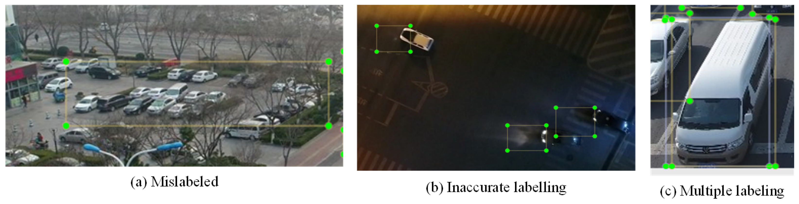
The visualization of misannotations in the UAVDT dataset. We employed LabelImg for visual inspection and manually removed these data points that could potentially affect the experimental outcomes.
Figure 5.
The visualization of misannotations in the UAVDT dataset. We employed LabelImg for visual inspection and manually removed these data points that could potentially affect the experimental outcomes.
Figure 6.
The OUC-UAV-DET dataset annotated using the Labelme tool.
Figure 6.
The OUC-UAV-DET dataset annotated using the Labelme tool.
Figure 7.
Visualization of the first layer after passing through the FCOS module and the first layer after passing through the FIEM module. The color red represents background learning, while the color blue represents object learning.
Figure 7.
Visualization of the first layer after passing through the FCOS module and the first layer after passing through the FIEM module. The color red represents background learning, while the color blue represents object learning.
Figure 8.
Error analysis was conducted on the proposed DroneNet (bottom row) and the baseline method (top row) across all ten categories using the validation set of VisDrone2021-DET. The horizontal axis represents the ground-truth labels, while the vertical axis represents the predictions. The confusion matrix displays the percentage of errors. This plot clearly illustrates the substantial enhancement in object identification ability achieved by our proposed DroneNet.
Figure 9.
The comparison of class activation visualizations between DroneNet and the baseline on the VisDrone dataset. Higher response values indicate higher predicted scores.
Figure 9.
The comparison of class activation visualizations between DroneNet and the baseline on the VisDrone dataset. Higher response values indicate higher predicted scores.
Figure 10.
A comparison of class activation visualizations between DroneNet and the baseline on three drone-view datasets, namely, VisDrone-2021, UAVDET, and OUC-UAV-DET, is presented. To enhance visual appeal, we utilize different colors to represent various categories.
Figure 10.
A comparison of class activation visualizations between DroneNet and the baseline on three drone-view datasets, namely, VisDrone-2021, UAVDET, and OUC-UAV-DET, is presented. To enhance visual appeal, we utilize different colors to represent various categories.
Table 1.
Assessing the impact of integrating our feature information enhancement module (FIEM), split-concat feature pyramid network (SCFPN), and coarse to refine label assign (CRLA) into the baseline on the validation of VisDrone2021-DET. The black bolded numbers indicate the current best results and the red numbers indicate how much improvement has been achieved compared to the baseline.
| FIEM | SCFPN | CRLA | mAP | Diff |
|---|
| | | | 21.2 | - |
| ✓ | | | 23.13 | +1.93 |
| | ✓ | | 24.52 | +2.98 |
| ✓ | ✓ | | 27.43 | +6.23 |
| | | ✓ | 25.13 | +3.93 |
| ✓ | ✓ | ✓ | 29.6 | +8.4 |
Table 2.
Comparison of the CRLA strategy with other label assignment strategies.The black bolded numbers indicate the current best results.
Table 2.
Comparison of the CRLA strategy with other label assignment strategies.The black bolded numbers indicate the current best results.
| Method | mAP |
|---|
| Baseline | 21.2 |
| +IOU | 20.35 |
| +SimOTA | 23.45 |
| +CRLA | 25.13 |
Table 3.
The analysis of different values of hyperparameter IoU threshold on the VisDrone validation set. The black bolded numbers indicate the current best results.
Table 3.
The analysis of different values of hyperparameter IoU threshold on the VisDrone validation set. The black bolded numbers indicate the current best results.
| IoU | 0.0 | 0.1 | 0.2 | 0.3 | 0.4 | 0.5 |
| mAP (%) | 28.18 | 28.84 | 29.6 | 29.16 | 29.02 | 27.78 |
Table 4.
The analysis of different values of hyperparameter K on the VisDrone validation set. The black bolded numbers indicate the current best results.
Table 4.
The analysis of different values of hyperparameter K on the VisDrone validation set. The black bolded numbers indicate the current best results.
| K | 6 | 7 | 8 | 9 | 10 | 11 | 12 | 13 | 14 | 15 |
| mAP (%) | 29.34 | 29.39 | 29.4 | 29.4 | 29.6 | 29.5 | 29.53 | 29.44 | 29.4 | 29.3 |
Table 5.
Experimental comparison of SCFPN modules. The black bolded numbers indicate the current best results.
Table 5.
Experimental comparison of SCFPN modules. The black bolded numbers indicate the current best results.
| | mAP | APs | APm | APl |
|---|
| FPN [35] | 20.49 | 9.2 | 23.4 | 32.1 |
| PAFPN [36] | 21.2 | 13.2 | 30.9 | 39.2 |
| BiFPN [37] | 22.31 | 10.2 | 26.9 | 38.7 |
| SCFPN | 24.52 | 12.4 | 32.4 | 42.9 |
Table 6.
Comparison of AP (%) on VisDrone, UAVDT, and OUC-UAV-DET by using our approach with various base detectors. The red numbers represent the highest precision, while the blue ones represent the second-highest precision.
Table 6.
Comparison of AP (%) on VisDrone, UAVDT, and OUC-UAV-DET by using our approach with various base detectors. The red numbers represent the highest precision, while the blue ones represent the second-highest precision.
| | VisDrone | UAVDT | OUC-UAV-DET |
|---|
| Method | mAP | AP50 | AP75 | APs | APm | APl | mAP | AP50 | AP75 | APs | APm | APl | mAP | AP50 | AP75 | APs | APm | APl |
|---|
| Faster R-CNN [22] | 21.9 | 37.1 | 22.7 | 13.1 | 33.6 | 27.2 | 81.4 | 98.3 | 95.5 | 74.5 | 86.5 | 89.9 | 38 | 63.2 | 40.3 | 24 | 42.6 | 44.8 |
| SSD [17] | 25.2 | 46.1 | 24.1 | 16.4 | 37 | 37.6 | 76.8 | 97.3 | 89.2 | 67.8 | 83.8 | 86.1 | 35.4 | 61.4 | 37 | 21.9 | 40.4 | 41.7 |
| RetinaNet [21] | 23.5 | 40.2 | 23.8 | 13.7 | 37.4 | 41 | 76.5 | 97 | 88.9 | 67.3 | 83.5 | 86.1 | 29 | 49.5 | 30.1 | 17.1 | 35.1 | 31.8 |
| Cascade R-CNN [24] | 24.5 | 39 | 26.1 | 15.2 | 36.7 | 39.2 | 84.2 | 98.6 | 96 | 76.7 | 88.6 | 92.7 | 39.2 | 63.8 | 42.1 | 25 | 43.7 | 46.5 |
| Libra R-CNN [39] | 21.7 | 36.7 | 22.4 | 13.4 | 32.6 | 34.6 | 81.1 | 96.7 | 95 | 71.8 | 85.6 | 90.1 | 37.7 | 63.1 | 40.1 | 23.7 | 42.3 | 44.9 |
| CenterNet [40] | 18.7 | 33.6 | 17.9 | 9.8 | 29.3 | 38.7 | 73.2 | 97.8 | 87.9 | 60.6 | 79.4 | 85.4 | 34.1 | 59.6 | 34.9 | 18 | 39.8 | 43.3 |
| HRNet [41] | 24.6 | 40.3 | 26.2 | 15.9 | 36.8 | 39.1 | 82.3 | 98.1 | 94.9 | 72.3 | 85.9 | 92.1 | 40.4 | 65.8 | 43.4 | 27.4 | 44.9 | 46 |
| TridentNet [42] | 20.7 | 35.3 | 20.9 | 12 | 30.9 | 37.5 | 79.9 | 98.6 | 94.3 | 71.8 | 85.2 | 90.8 | 36.8 | 62.1 | 38.4 | 21.2 | 42 | 45.2 |
| FCOS [43] | 19 | 31.9 | 19.7 | 10.2 | 29.1 | 38 | 80.8 | 98.9 | 94.7 | 72.8 | 85.7 | 89.6 | 36.3 | 61.4 | 37.6 | 21.2 | 41.6 | 43.6 |
| FSAF [44] | 20.8 | 36.4 | 20.5 | 13.3 | 29.3 | 34.7 | 82.1 | 98.8 | 95.3 | 74.2 | 85.9 | 91.6 | 34.5 | 59.2 | 35.4 | 20.7 | 38.7 | 40.2 |
| Sabl [45] | 21.9 | 36 | 22.9 | 12.9 | 33.1 | 33.8 | 84.1 | 98.3 | 96.4 | 76.3 | 88.6 | 92.3 | 38.8 | 63 | 41.6 | 24.4 | 43.6 | 46.9 |
| VFNet [46] | 23.1 | 37.3 | 24.1 | 14.2 | 33.9 | 39.4 | 85.5 | 98.9 | 97.4 | 79.2 | 89.1 | 91.7 | 39.8 | 64.2 | 42.2 | 24.5 | 45.6 | 46.8 |
| TOOD [10] | 24.4 | 39.8 | 25.3 | 15.5 | 35.5 | 41.4 | 86.5 | 99 | 97.8 | 81.6 | 89.3 | 93 | 40 | 64.8 | 43 | 25.6 | 44.9 | 45.8 |
| DDOD [47] | 23.3 | 38.2 | 24.2 | 14.4 | 34.5 | 39.6 | 85.1 | 98.9 | 97.5 | 78.9 | 88.2 | 92.8 | 39.1 | 64.1 | 41.5 | 24.2 | 44.3 | 46.2 |
| ObjectBox [48] | 22.5 | 39.9 | 22.1 | 13.4 | 34.2 | 38.8 | 86.9 | 98.3 | 98.1 | 81.4 | 89.1 | 93.4 | 46.5 | 71.3 | 50.7 | 34.7 | 50.4 | 51 |
| YOLOv3 [20] | 24.8 | 43.9 | 24.2 | 16.5 | 34.4 | 45.2 | 87.5 | 98.4 | 97.2 | 83 | 89.9 | 93.5 | 46.4 | 71.3 | 50.8 | 34.5 | 50.7 | 50.9 |
| YOLOv4 [49] | 23.5 | 39.2 | 23.4 | 13.3 | 35.4 | 45.1 | 87.9 | 98.1 | 97.5 | 82.5 | 89.7 | 93.2 | 43.2 | 66.4 | 46.1 | 28.8 | 47.2 | 48.9 |
| YOLOX [31] | 22.4 | 39.1 | 22.3 | 13.7 | 33.1 | 41.3 | 87.7 | 97.9 | 97.4 | 83.2 | 89.2 | 93.4 | 47.1 | 72 | 51.5 | 34.8 | 51.4 | 52.2 |
| YOLOv6 [50] | 27.1 | 44.5 | 27.7 | 17 | 40.1 | 47.1 | 88.1 | 98.7 | 97.5 | 82.9 | 89.6 | 92.4 | 46.8 | 71.6 | 51.6 | 33.9 | 50.9 | 51.7 |
| YOLOv7 [11] | 27.9 | 48.3 | 27.5 | 18.5 | 39 | 49.3 | 88.6 | 99.1 | 98.2 | 83.1 | 90.2 | 93.6 | 47.4 | 72.9 | 52.3 | 34.3 | 51.7 | 53.4 |
| YOLOv8 [51] | 25.9 | 42.9 | 26.4 | 16.6 | 38.2 | 45.8 | 87.5 | 98.2 | 97.1 | 82.4 | 89.3 | 93.1 | 46.3 | 71.1 | 51.2 | 34.1 | 50.6 | 51.6 |
| Baseline [38] | 21.2 | 37.3 | 20.8 | 13.2 | 30.9 | 39.2 | 88.2 | 98.5 | 97.5 | 82.9 | 90.1 | 93.1 | 45.9 | 70.7 | 50 | 32.7 | 50.7 | 51.1 |
| DroneNet | 29.6 | 50.4 | 29.6 | 19.9 | 41.9 | 49.6 | 89.1 | 99.4 | 98.9 | 83.7 | 91.2 | 94.6 | 48.8 | 73.3 | 53.2 | 35.8 | 52.9 | 54.8 |
Table 7.
DroneNet, combined with sliding window crop method, is compared to various object detection strategies involving image cropping on the Visdrone validation set. The black bolded numbers indicate the current best results.
Table 7.
DroneNet, combined with sliding window crop method, is compared to various object detection strategies involving image cropping on the Visdrone validation set. The black bolded numbers indicate the current best results.
| Method | AP | AP50 | AP75 |
|---|
| UCGNet [52] | 32.8 | 53.1 | 33.9 |
| ClusDet [25] | 32.4 | 56.2 | 32.6 |
| GLSAN [53] | 32.5 | 55.8 | 33 |
| PRDet [14] | 38.6 | 60.8 | 40.6 |
| DroneNet (+Crop) | 39.11 | 62.1 | 42.5 |
Table 8.
The speed performance comparison of DroneNet with the baseline model and TPH-YOLOv5 was conducted on the VisDrone dataset, using a 2080ti GPU. The black bolded numbers indicate the current best results.
Table 8.
The speed performance comparison of DroneNet with the baseline model and TPH-YOLOv5 was conducted on the VisDrone dataset, using a 2080ti GPU. The black bolded numbers indicate the current best results.
| Method | mAP | FPS |
|---|
| Baseline [38] | 21.2 | 84.74 |
| TPH-YOLOv5 [27] | 25.73 | 68.4 |
| DroneNet | 29.6 | 84.03 |


 and
and 


