1. Introduction
We consider a class of missions in which a set of mandatory tasks must be completed by a pair of Unmanned Vehicles (UVs) with the minimum energy consumption. The nature of the tasks is mission-specific and can range from capturing images and video streams to extinguishing fires and neutralizing mines [
1,
2,
3,
4]. Each task is situated at a geographically distinct (and stationary) location, referred to as a target, in a potentially hazardous environment. UVs are chosen for this mission due to their high mobility, ability to perform diverse sets of tasks and navigate in hazardous environments, and low costs [
5,
6,
7]. Due to the nature of the environment, at every target, the UV performing the task, referred to as the leader, is required to communicate with another UV, referred to as the wingmate, which is expected to be in close proximity. This helps the UVs to protect each other from threats associated with the environment or the task, establish stealth communication with a low probability of detection or jamming [
8,
9,
10], exchange large volumes of data at a low cost, and complete tasks in the event of a failure of the original task performer. Such missions have applications in the fields of surveillance and reconnaissance, wildfire fighting, and exploration of unknown environments.
In this paper, we consider the problem of determining the task allocations to the UVs and the sequences for the UVs to visit the targets such that the energy consumed by the vehicles is minimized. We assume that the sequence of task completion does not influence the energy consumed for performing tasks and onboard computations. Then, the problem objective reduces to minimizing the energy consumed for travel and communication. The actual amount of energy consumed for travel depends on several external factors such as wind conditions and ambient temperature, in addition to the distance traveled by the UVs. However, owing to the complexity involved in developing such high-fidelity models and the computational challenges involved in employing them in planning problems, we adopt a widely used simplification from the literature of route planning. Specifically, we use the distance traveled by the UVs as a proxy for the energy consumed during travel. Similarly, we use the distance between the UVs while communicating as a proxy for the energy consumed for communication tasks.
With these simplifications, the planning objective reduces to that of minimizing a weighted sum of the travel and communication distances, where the weights account for mission-specific priorities and the differences in the characteristics of travel and communication costs. Nevertheless, the planning problem with the weighted objective remains computationally challenging, as will be discussed in
Section 4.2. Furthermore, the literature on algorithms to solve this problem is sparse, as will be discussed in
Section 2. Therefore, as a first step toward filling this void, in this paper, we focus on developing algorithms to solve the problem with equal weights assigned to the travel and communication distances. Later, we show that these algorithms can be extended to the weighted case and discuss one such extension.
In the context of mission planning, the problem considered here is important because there is a trade-off between minimizing travel costs and communication costs. Focusing solely on minimizing travel costs may result in routes with large distances between communicating vehicles. This poses challenges as it can lead to increased energy consumption for communication tasks and the potential depletion of UVs’ fuel or charge before completing all tasks and returning safely. Particularly in missions involving the exchange of large volumes of data, longer distances between vehicles hinder efficiency. Additionally, in surveillance applications where stealth is crucial, greater distances between communicating vehicles increase the risk of detection or interference. On the other hand, prioritizing communication cost minimization can lead to routes requiring UVs to travel longer distances, which increases the risk of energy depletion. This can be further exacerbated by unfavorable wind conditions. Therefore, there is a need for jointly minimizing travel and communication costs.
1.1. Operational Setup
To formalize the problem statement in accordance with the above discussion on the requirements of tasks and UV communications, we consider the following operational setting for the vehicles. We assume that there are an even number of tasks and that all the tasks are mandatory. Each UV is assigned an equal number of tasks. While a task can be assigned to either UV, each task must be assigned to exactly one vehicle. Along with a set of tasks, each UV is provided a sequence in which the tasks must be performed. These sequences translate to tours over all the targets corresponding to the assigned tasks. Given a task allocation and tours for visiting the targets, each UV starts at the first target in the tour. At every target, the UVs are required to communicate with their partner before traveling to the next target in their assigned tour. For example, the first UV can leave the i-th target in its tour only after the second UV has reached the i-th target of its own tour and both the vehicles have communicated. To satisfy this communication requirement in the real world, the UVs can either hover at their current targets and gather additional information until their partner reaches its respective target or change speeds such that they reach their respective targets at the same time. The former coordination scheme might be easier to implement in practice. This coordination continues until the end of the mission, which is marked by both UVs returning to their starting targets.
1.2. Problem Statement
Given a pair of UVs and an even number of tasks for them to complete, the aim of the problem is to (1) determine an allocation of these tasks to the UVs, and (2) plan tours for the UVs to visit targets at which the tasks are located, such that the operational constraints mentioned in
Section 1.1 are satisfied, and the weighted sum of the combined distances traveled by the UVs and the distances between the UVs while communicating at the targets is minimized.
1.3. Contributions
To facilitate the computation of high-quality solutions to this problem, we make the following contributions in this paper with a focus on the case with equal weights assigned to the travel and communication distances.
In
Section 3, we formulate the problem of determining task allocations and routes for the UVs that minimize the weighted sum of the travel and communication distances as an Integer Program.
In
Section 4.2, we demonstrate the computational challenges involved in naively solving the formulation using commercial off-the-shelf solvers.
In
Section 5, we develop an approximation algorithm to solve the problem and show that the algorithm has an approximation ratio of 3.75 for the case with equal weights assigned to the travel and communication distances.
In
Section 5.3, we develop a heuristic algorithm with distinct advantages to complement the approximation algorithm in computing solutions for the equally-weighted case.
In
Section 5.2, we develop a lower bound to the optimal cost of the equally-weighted problem to help in evaluating the quality of available feasible solutions.
In
Section 6, we present the results of extensive numerical experiments performed on the equally weighted case of the problem using 500 instances. Using these results, we evaluate the performance of the proposed algorithms and highlight their advantages and use cases.
In
Appendix A, we show that the approximation algorithm proposed in
Section 5 has a variable approximation ratio for the general weighted case. Specifically, by defining
as the ratio of the weights assigned to the communication and travel distances, the algorithm has a ratio of
when
, and
when
.
2. Literature Review
In multi-vehicle missions, communication between the vehicles plays a crucial role in enhancing coordination, safety, and situational awareness. However, surprisingly, a majority of the literature on multi-vehicle route planning has neglected the communication requirements of the vehicles and focused solely on minimizing their travel costs [
11,
12,
13]. Communication-aware route planning has been considered in articles [
14,
15,
16,
17,
18], where the vehicles are allowed varying levels of flexibility in communication. In articles [
14,
15], the authors plan routes for multiple vehicles that minimize the travel costs of the vehicles while ensuring that each vehicle is connected with every other vehicle performing the mission at all times, either directly by being within the communication range or in a multi-hop manner by relaying messages through other vehicles. In [
16], the authors consider a similar connectivity requirement but consider the problem of minimizing the number of vehicles required for task completion. In [
17], the authors allow a flexible operation, where the UVs are not required to stay connected with each other at all times. Instead, the UVs are allowed to spread out to perform certain tasks and intermittently reconnect with each other to exchange information. In this article, the authors consider the problem of minimizing the travel cost of the paths taken by the UVs to reconnect with each other. In [
18], the UVs are allowed to break connectivity after initially starting the mission in a connected configuration. However, they are required to regain the initial connected configuration at periodical time intervals. With these communication requirements, the authors consider the problem of path planning for multiple vehicles such that the information gained by visiting a set of targets is maximized. In [
19], the authors consider a communication framework in which data are exchanged between UVs traveling on distinct tours to ensure that the collected data are eventually transferred to a base station. To facilitate such an exchange, the UVs wait at pre-determined locations in their tours until their partner arrives. In this article, the authors consider the problem of minimizing the travel cost of the largest tour.
The problem considered in the current paper has similarities to [
18,
19] in the communication framework considered. Specifically, similar to [
18], the UVs in the current article are not required to be connected at all times. Instead, the UVs are required to communicate with each other only when they reach a target. Likewise, similar to [
19], the UVs in the current article wait for their partner to arrive at the scheduled locations to exchange information. However, unlike [
19], the UVs in the current paper need to coordinate their visits and exchange information at every target. Furthermore, the problem considered in the current article differs fundamentally from all the aforementioned articles, including [
18,
19], due to its objective. Here, it is not sufficient to ensure that the vehicles are either connected or within a communication range. Instead, the objective here is to minimize the energy consumed by the vehicles for communication along with that consumed for travel. This objective has the advantage of providing routes that lower the mission costs and improve communication quality. Additionally, articles [
20,
21] show that traveling is not necessarily the major consumer of a UV’s energy and including the energy consumed for communication tasks in the planning phase can result in higher energy savings and increased flight time.
Minimal energy route planning has been considered in the context of planning paths for a single UV in [
21,
22,
23], where the vehicle is required to communicate with one or more remote base stations to transmit the collected data. Specifically, in [
22], the authors consider a point-to-point path planning problem for a single UV that utilizes a cellular network to communicate video streams to a base station. In this problem, given a cellular coverage map and a budget on energy consumption, the objective is to determine paths for the UV between a specified source and a destination such that the communication quality is maximized. In [
21], the authors consider a similar setup in which a single UV is required to communicate with one or more base stations while traveling from a source to a destination through a set of other specified waypoints. Here, the objective is to determine paths that minimize the total energy consumption. In this article, the authors show that paths that include the energy consumed for communication result in overall energy savings and extend the flight time of the UV when compared to paths that neglect communication costs. In [
23], the authors consider a path planning problem in which a single UV is required to visit a set of targets and then find an optimal location in the environment to wirelessly communicate the data collected from the targets to a base station. The objective of the problem is to determine paths for the UVs to the targets and the data transfer location such that the sum of the travel and communication costs is minimized.
The current article differs from those mentioned in the previous paragraph in the following ways: (1) this article considers multiple UVs, (2) the routes considered in this paper are tours as opposed to paths, which makes the planning problem challenging, (3) there is no base station close to the mission environment, and the UVs are required to exchange information with each other as opposed to transmitting the collected data to a base station. While [
24] considers the problem of planning minimal energy tours for multiple UVs, the UVs therein do not communicate with each other. Instead, similar to [
21,
22,
23], the UVs in [
24] are required to transfer the collected data to a remote base station either immediately or in an aggregated manner by selecting a location along the UVs’ trajectory to transfer the data collected from all the targets. To the best of our knowledge, there are no algorithms in the literature that address the problem of minimizing travel and communication costs with the communication framework considered in this paper.
3. Mathematical Formulation
We formulate the route planning problem as a network optimization problem, which takes the form of an Integer Program (IP), on a complete graph, . The vertex set, V, represents the targets to be visited by the UVs, the edge set, E, represents the travel/communication paths between every target pair, which is assumed to be a straight line connecting the targets, and the edge weights, , represent the Euclidean distances between the targets (lengths of travel/communication paths). We assume that the communication path between every target pair is the same as the travel path between the pair and therefore, they are represented by the same edge in the graph. Furthermore, the edge weights obey the triangle inequality.
In this representation, the desired solution is a connected graph with every vertex having a degree of 3; two incident edges represent the travel paths of the UVs through the target and one incident edge represents the communication link formed by a UV while present at the target. The set of edges in the solution describes the sequence in which the UVs must visit the targets and the communication links formed between the vehicles while they are present at the targets. The mathematical description of the IP that is used to compute such a solution with the minimum travel and communication costs is presented below.
3.1. Data
| Number of targets in the environment |
| Euclidean distance between targets i and j, where |
| Weight assigned to the travel distances in the objective function |
| Weight assigned to the communication distances in the objective function |
3.2. Variables
We use six sets of binary variables to capture the vehicle’s target assignment, and travel and communication paths. First, the set of binary variables
,
, is used to indicate if a target is assigned to the first UV, i.e., UV-1, or the second UV, i.e., UV-2. Note that the numbering of the UVs can be arbitrarily chosen.
Then, we use the set of variables
to indicate whether UV-1 is required to traverse a path
between targets
i and
j, where
.
Similarly, we use the set of variables
to indicate whether UV-2 is required to traverse a path
between targets
i and
j, where
.
Next, the set of variables
is used to indicate whether an edge
, where
, is utilized by the UVs for communication at any point in time in the mission.
Finally, we utilize the sets of variables
and
,
, and
, to define pairs of travel and communication edges, which will be helpful in enforcing communication links such that they obey the sequence in which the UVs visit the targets. Specifically,
models the presence of a travel edge for UV-1 between targets
i and
j and a communication link between targets
j and
l. That is,
Similarly,
models the presence of a communication edge between targets
i and
k, and a travel edge for UV-2 between targets
k and
l. That is,
More on utilizing these variables to model the proper enforcement of communication links will be discussed in the following subsection.
3.3. Constraints
Using these binary variables, the problem requirements can be represented as mathematical constraints as follows.
3.3.1. Target Assignment
Each UV must be assigned exactly
m targets. This is represented by Equation (
1).
3.3.2. Feasible Tours/Sequences
A UV can traverse between two targets (along an edge with the targets as the endpoints) only if both the targets are assigned to the UV. Constraints (
2) and (
3) ensure that an edge,
, is assigned to UV-1’s tour only if targets
i and
j are both assigned to UV-1, and constraints (
4) and (
5) ensure that an edge
is assigned to UV-2’s tour only if both
i and
j are assigned to UV-2.
The purpose of constraints (
6) and (
7) is to ensure that a UV visits a target exactly once if the target is assigned to it and never if the target is not assigned to it.
Constraints (
8) and (
9) ensure that a UV arriving at a target must also depart from the target.
In addition to the aforementioned degree/flow requirements, a UV’s path is required to be connected and must not contain sub-tours. This can be enforced by constraints (
10) and (
11), which are referred to as sub-tour elimination constraints [
25,
26].
Even though these constraints are exponential in number, we prefer this representation of the sub-tour elimination constraints due to the tighter relaxation it offers compared to its alternatives [
27]. Nonetheless, we discuss an efficient implementation of this exponential number of constraints in
Section 4.1.
3.3.3. Communication Links
Once the UVs’ travel paths are determined, the communication links can be described using the set of constraints (
12)–(
22). Firstly, the UVs communicate only once at every target. This is expressed by the set of inequalities (
12).
Because every UV visits exactly
m distinct targets, there are a total of
m communication links; this is captured by Equation (
13).
Then, as communication occurs between two distinct vehicles, there are no communication links between targets assigned to the same UV. This is captured by the sets of inequalities described by (
14) and (
15).
Next, the communication links must be constrained such that they are consistent with the sequence in which the targets are visited by the UVs. We explain the modeling of such constraints using
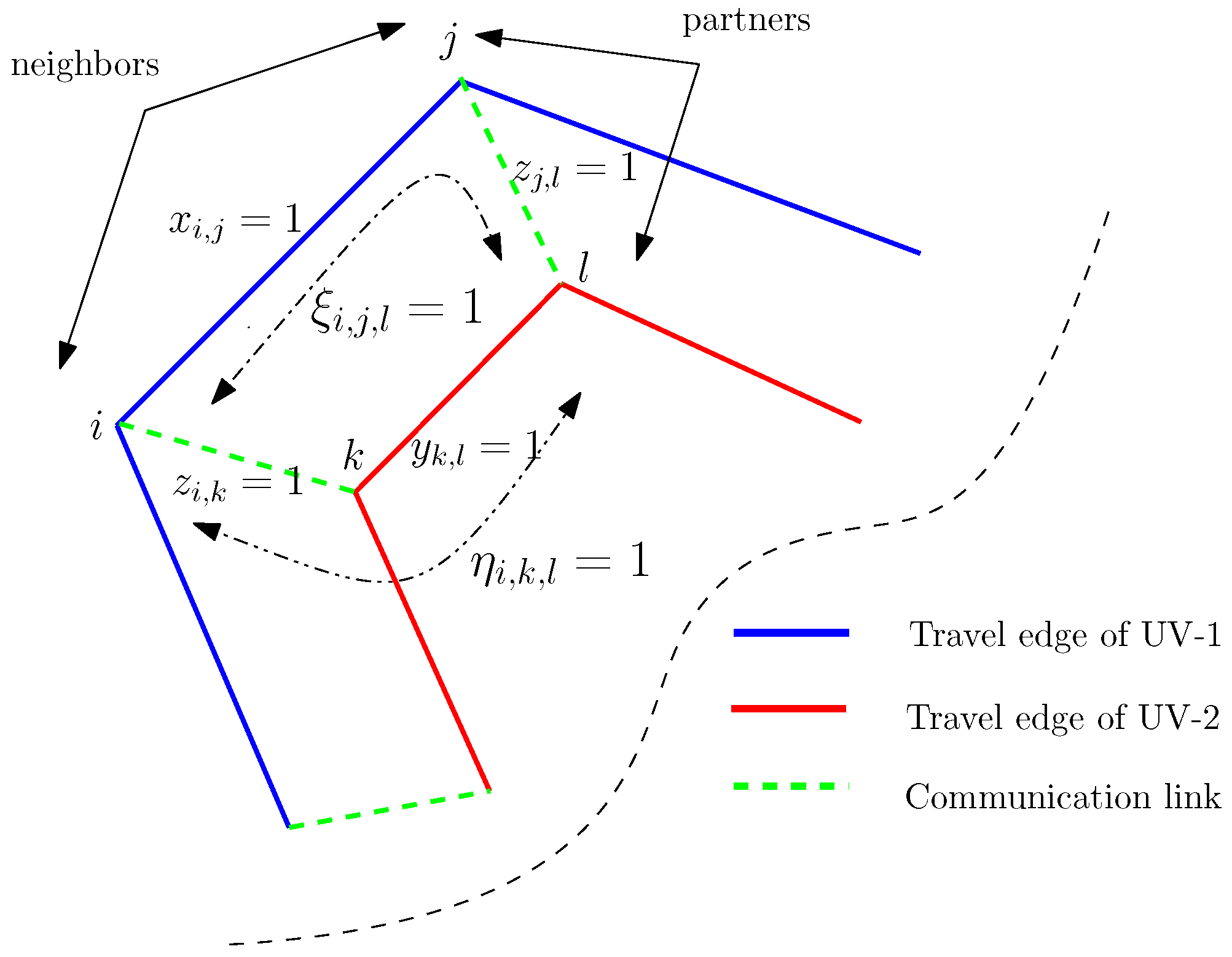
Figure 1. This figure illustrates two tours for the UVs and the communication links between them; the outer tour (in blue) is assigned to UV-1, the inner tour (shown in red) is assigned to UV-2, and the green dotted lines depict the communication links. For ease of exposition, we will refer to a pair of targets that share a travel edge as neighbors and a pair of targets that share a communication edge as partners. Then, it can be observed from the figure that the communication links obey the travel sequence of the UVs if and only if the neighbor’s partner of every target is also its partner’s neighbor. To elaborate, consider target
i in
Figure 1. Observe that target
j is a neighbor of
i and target
l is a partner of
j. That is,
l is the partner of a neighbor of
i. Note that
l can also be considered as the neighbor of target
k, which is in turn the partner of
i. That is,
l is also a neighbor of the partner of
i. The same argument can be applied to every target in the vertex set. In other words, the communication links are consistent with the travel sequence if and only if the following statement holds true: for two arbitrarily chosen distinct targets, say
i and
in the vertex set, the latter is the neighbor’s partner of the former if and only if the latter is also the partner’s neighbor of the former.
To model the neighbor’s partner and partner’s neighbor of targets, we utilize the variable sets
and
, respectively. Specifically,
takes the value 1 if
i is assigned to UV-1,
j is a neighbor of
i (i.e.,
), and
l is the partner of
j (i.e.,
); it takes the value 0 otherwise. The same is modeled using constraints (
16).
Similarly,
takes the value 1 if
i is assigned to UV-1,
k is the partner of
i (i.e.,
), and
l is a neighbor of
k (i.e.,
); it takes the value 0 otherwise. This is modeled using constraints (
19).
Then, the condition of a target (say
l) being the neighbor’s partner of the other (say
i) if and only if it is also the partner’s neighbor (of
i) can be represented by Equation (
22).
3.4. Objective
From the tours and communication links that satisfy the aforementioned constraints, the objective of the problem is to find the ones that minimize the total energy consumed by the UV for travel and communication. This translates to minimizing the weighted sum of the lengths of all the selected edges and can be mathematically represented by (
23).
The objective function (
23), together with constraints (
1)–(
22), defines the integer program of interest.
When the weights assigned to the travel and communication distances are equal, we have that
. Then, the problem can be equivalently solved by minimizing the unweighted objective given by (
24).
4. Computing Optimal Solutions
4.1. Implementation
We implemented this integer program in Julia, using JuMP, a package for mathematical optimization. Then, given an instance of the problem with target locations specified, we first evaluate the function , , by computing the Euclidean distances between the targets. Then, we solve the integer program for the instance using the branch and bound method in Gurobi, a commercial off-the-shelf optimization solver that is known to be one of the best in handling integer programs.
It is to be noted that the number of constraints specified by the inequalities (
10) and (
11) is an exponential function of
m, and directly adding such a large set of constraints to the problem makes solving it difficult. Therefore, we adopt a lazy callback approach [
28], where we first solve the problem without the sub-tour elimination constraints, and then iteratively add only the violated sub-tour elimination constraints and re-solve the problem until a solution that satisfies all the constraints is obtained; this solution is optimal to the problem.
4.2. Computation Time
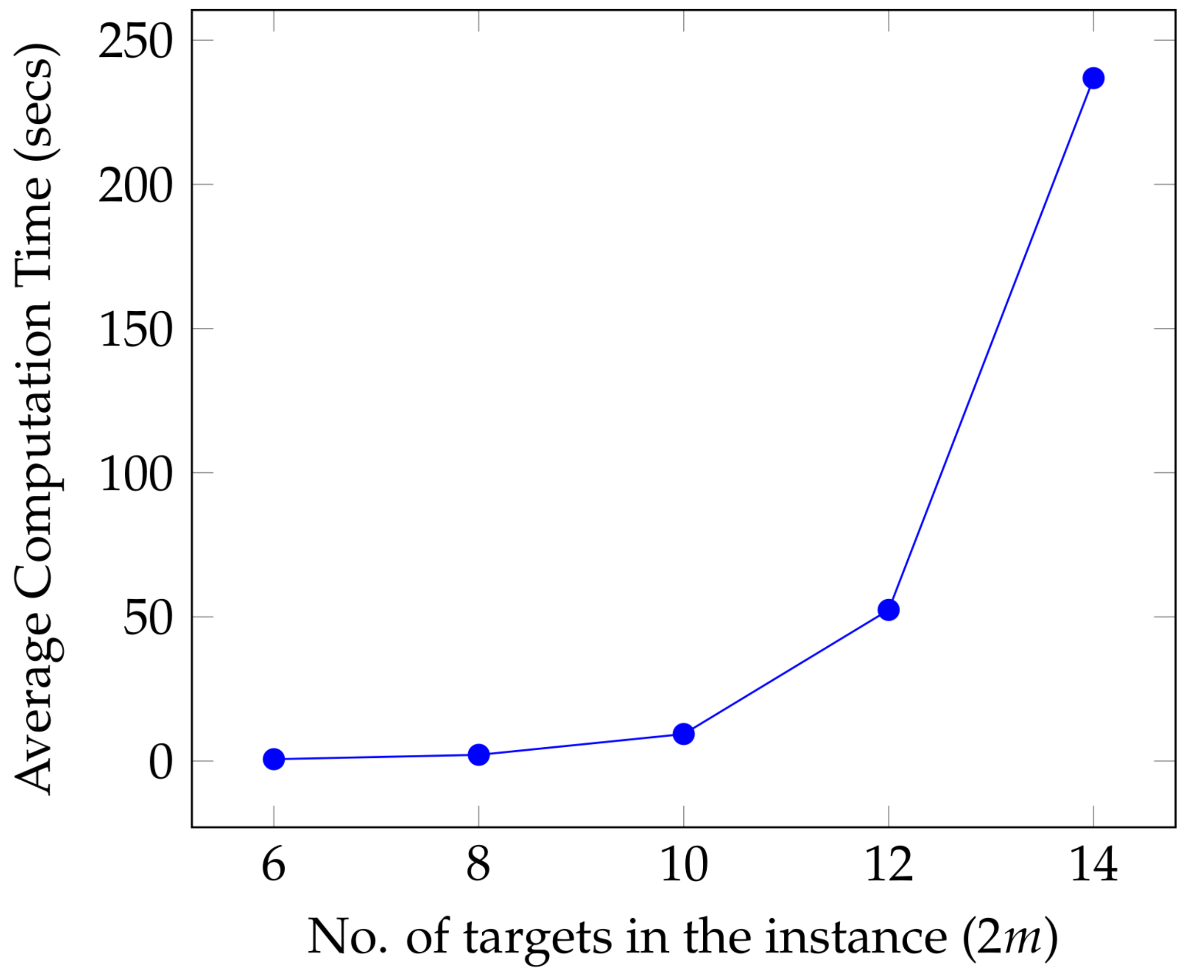
We used this procedure to solve the equally weighted case of the problem for 300 randomly generated instances, with the number of targets in these instances ranging from 6 to 16; there are 50 instances each with 2
m = 6, 8, 10, 12, 14, and 16. The simulations suggest that the average computation time required to solve the problem increases rapidly with the number of targets in the instance; the average computation time (taken over 50 instances) against the number of targets in the instance is shown in
Figure 2. The solver was unsuccessful in providing optimal solutions for instances with
within a 3 h cut-off time.
This suggests that generic methods to solve the integer program are insufficient to compute optimal solutions for large-scale instances of this problem, even when the weights assigned to the travel and communication distances are equal. Therefore, there is a need for developing algorithms that are tailor-made to solve this problem. For this reason, in this work, we first focus on the equally weighted case and develop approximate and heuristic algorithms to compute good-quality solutions to the problem swiftly. Then, we present a discussion on the applicability of these algorithms to the general weighted case in
Appendix A. Unless otherwise mentioned, the rest of the discussion presented in the paper is focused on the equally weighted case.
5. Approximation Algorithm
An approximation algorithm provides solutions with a worst-case guarantee on their quality. The quality of the solution is determined by the approximation ratio, which is the ratio of the worst-case cost of the solution provided by the algorithm to the cost of the optimal solution to the problem. Furthermore, the computation time required for implementing an approximation algorithm must be a polynomial function of the input size, i.e.,
m. Here, we develop such an algorithm for the equally weighted case with a fixed approximation ratio of
. It will be shown in
Appendix A that this algorithm has a variable approximation ratio for the general weighted case.
5.1. Algorithm
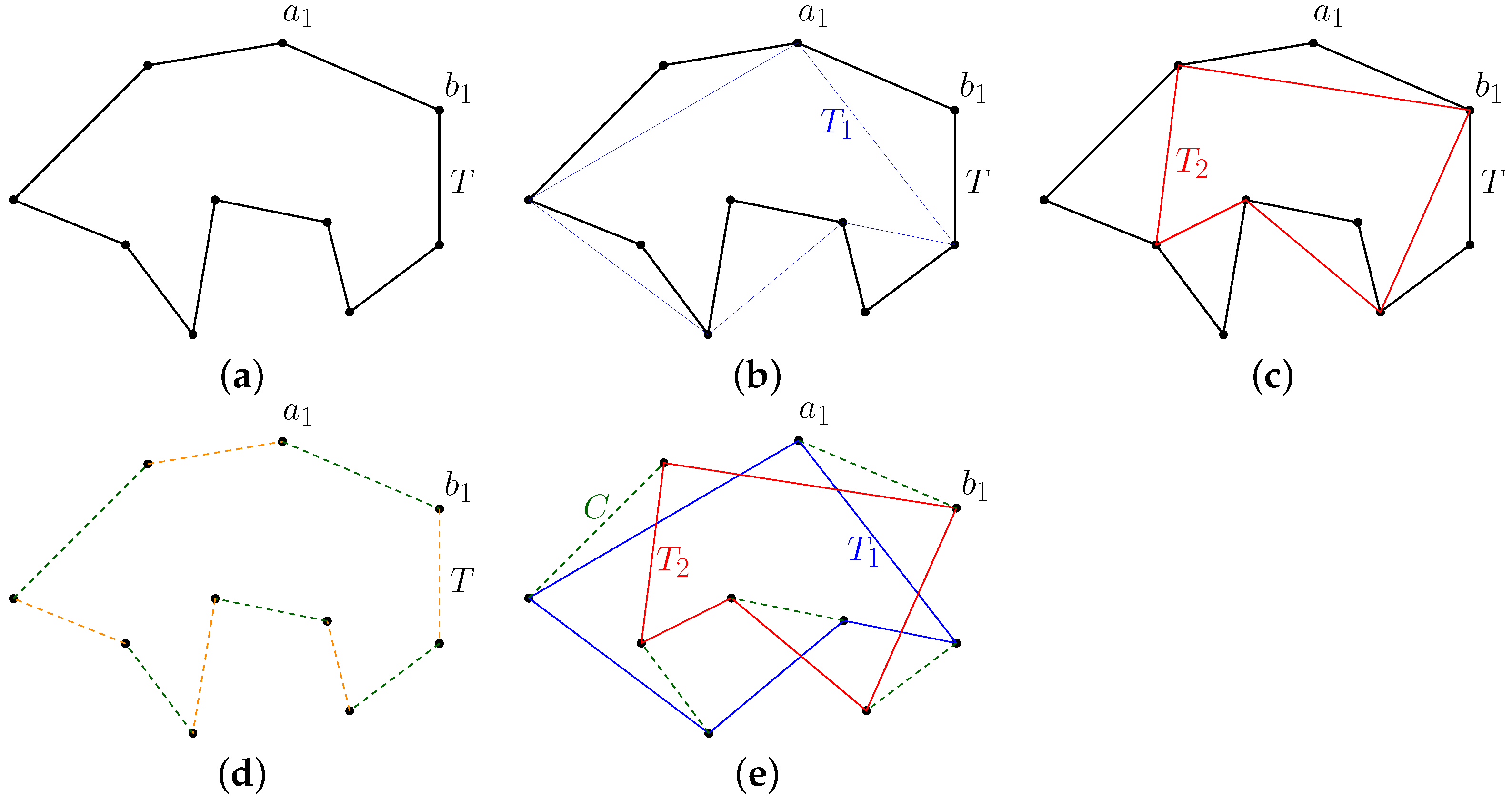
We illustrate the steps of the algorithm on a 10-target instance shown in
Figure 3. The first step of the algorithm involves computing a single UV tour over all the targets in the environment, i.e., a tour that allows a single UV to start at a target, visit all the targets once, and return to the starting point. Such a tour of the minimum travel cost is an optimal solution to the classic Traveling Salesman Problem (TSP). Here, we utilize the well-known Christofides algorithm [
29], an approximation algorithm to the TSP with an approximation ratio of 1.5, to compute the desired single UV tour. This step has a time complexity of
[
30]. Let this tour be denoted by
T;
Figure 3a illustrates a single UV tour spanning all the 10 targets. We tailor this tour to construct the desired feasible tours for both the UVs and the communication links between them.
The next step of the algorithm provides feasible tours for both the UVs in the mission. To obtain the tour for the first UV, pick any vertex, say
, from
T. Then, starting at
, construct a graph by joining only the alternate vertices of
T, as shown by the blue edges in
Figure 3b; denote the constructed graph by
. In other words,
is a tour obtained by skipping visits to alternate vertices from
T.
is the desired tour for the first UV in the mission, covering half of the targets in the environment. Now, consider the vertex
, adjacent to
, in
T. Then, similar to the construction of
, construct a graph starting at
and skipping alternate vertices of
T, as shown in
Figure 3c; denote the obtained graph by
.
represents the desired tour for the second UV in the mission, covering the rest of the targets. This step of the algorithm has a time complexity of
.
The final step of the algorithm involves identifying the communication links between the vehicles when they visit their respective targets. Thus far, we have feasible tours for both UVs, but the starting points of the UVs in their tours are not yet determined. This leaves us with a number of options from which the communication links can be chosen. In this algorithm, we restrict the communication links to the set of edges of
T. In that case, the two sets of alternating edges of
T are candidate communication links—either the set containing the edge
, shown in green in
Figure 3d, or the set that does not contain this edge, shown in orange in
Figure 3d. From these two sets, we choose the set that has the minimum sum of the costs of all its edges. Let this set of edges be
C. This step has a time complexity of
. Then,
,
, and
C together constitute the solution of the algorithm and it is a feasible solution to the problem; the solution of the algorithm for the illustrative instance is shown in
Figure 3e. Overall, the algorithm has a time complexity of
.
It is to be noted that all the steps of the algorithm can be performed in a polynomial time. Next, to obtain worst-case guarantees, we need to analyze the cost of the solution obtained from this algorithm.
Cost of Solutions
The cost of the solution of this algorithm is the sum of the costs of the edges of
,
, and
C, i.e.,
. Let us analyze the edge costs of these graphs individually. Firstly, recall that the sum of the cost of edges of
T is at most
, where
is the cost of an optimal TSP tour over the targets. This follows from the approximation ratio of the Christofide’s tour
T [
29]. Then, recall that
and
are obtained by skipping or shortcutting visits from
T. Then, due to the triangle inequality of edge costs, it follows that the sum of the costs of edges of
is at most that of
T. That is,
. Since the construction of
is similar to that of
T, we have that
.
Now, recall that
C is the set of alternating edges of
T that has the minimum cost. Let the costs of alternating edges of
T aggregate to
and
. Then,
. WLOG, suppose that
. Then, we have that
. Combining these, it follows that
Therefore,
. Consequently, the cost of the solution provided by the algorithm can be upper-bounded as follows:
The quality of a feasible solution to the problem is usually evaluated by the gap between the solution cost and the optimal cost. A lower gap indicates that the solution is near-optimal and a higher gap indicates that the solution is sub-optimal. However, in cases where the optimal cost is unavailable, a lower bound to the optimal cost that is relatively easier to compute is useful in estimating the solution quality. A lower gap between the solution cost and the lower bound indicates that the solution is near-optimal (optimal if the gap is zero). Nevertheless, a higher gap does not necessarily mean that the solution is far from optimality. It can indicate that the lower bound is not binding and can be improved. Here, we develop a lower bound to the optimal cost that helps in establishing the worst-case cost of the algorithmic solution, also known as the approximation ratio. The lower bound can also be used to evaluate the quality of any other feasible solutions to the problem.
5.2. Lower Bound to the Optimal Cost
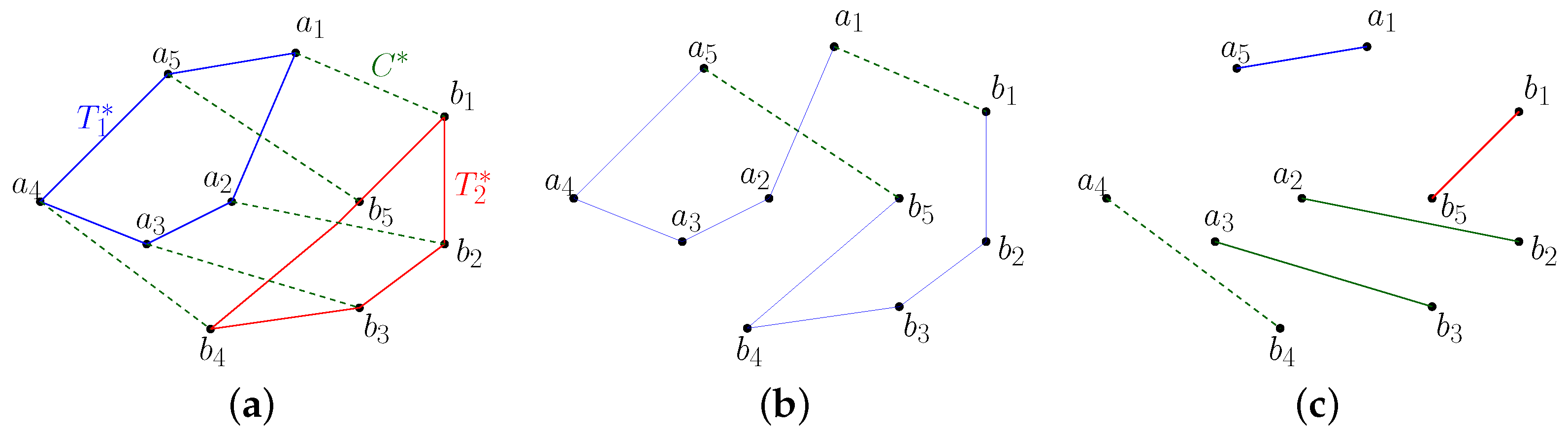
Let
be an optimal solution, where
and
are the tours obtained by traversing the targets in the orders specified by the following tuples, respectively:
,
, and
denotes the set of communication links, as shown in
Figure 4a. Now, from
, consider only the edges obtained by traversing across all the vertices in the specified order:
. These edges form a single UV tour over all the targets, as shown in
Figure 4b. Therefore, the cost of these edges is at least
. Next, observe that the rest of the edges in
, i.e.,
, form a perfect bi-partite matching, as shown in
Figure 4c. Therefore, the cost of these edges is at least equal to
, which is the cost of the minimum weighted perfect bi-partite matching of
G. As a result,
is a valid lower bound for the cost of the optimal solution. We will use this lower bound in
Section 6 to evaluate the quality of the algorithmic solutions developed in this paper.
From the lower bound, it follows that
Then, combining inequalities (
25) and (
26), we have that
is an approximation ratio of the algorithm. This ratio is also referred to as the a priori ratio.
5.3. Heuristics
If the solve time being a polynomial function of the input size is not a requirement, in the first step of the algorithm, one can use an alternative single UV tour with a lower cost. For example, one can use a tour
T obtained from the Lin–Kernighan heuristic [
31], which is known to provide near-optimal solutions to the TSP for many instances quickly. This helps in improving the quality of the solutions.
6. Results
In this section, we evaluate the performance of the proposed heuristic and approximation algorithms by presenting the results of numerical experiments performed on 500 instances of the problem. The instances were created by randomly generating target coordinates over a 500 × 500 grid (using the rand function in Julia). The number of targets in these instances ranges from 6 to 100, with exactly 50 instances each with
, 8, 10, 12, 14, 20, 30, 40, 50, and 100. All computations presented in this paper were performed on a MacBook Pro with 16 GB RAM and Dual-Core Intel Core i7 processor @ 2.8 GHz. Besides the computation of the LKH tours, for which the software package [
32] was used, all the algorithms were implemented in Julia. Optimal solutions were computed by implementing the formulation presented in
Section 3 using JuMP, a Julia package for mathematical programming, and solving the formulation using Gurobi [
33], a commercially available optimization solver. Depending on the computation time required to determine optimal solutions, the 500 instances were divided into two sets: (1) the set of small instances comprising instances with a computation time of at most 3 h, and (2) the set of large instances comprising instances for which optimal solutions were not computable within the 3 h cutoff time. The former set consists of 250 instances with
, whereas the latter set consists of the remaining instances with
.
To evaluate the performance of the algorithms, we consider two criteria: (1) the quality (cost) of the solutions provided by the algorithm, and (2) the time taken to compute these solutions. A desirable algorithm provides good-quality solutions quickly. We use two indicators to evaluate the quality of the solutions. The first indicator is the a posteriori ratio, which is the ratio of the cost of the algorithmic solutions to the cost of the optimal solution. Note that this is different from the a priori ratio (also known as the approximation ratio), which is the worst-case bound on the a posteriori ratio. Even though the a posteriori ratio is an accurate metric to evaluate the solution quality, it cannot be computed when the optimal cost is not available and therefore cannot be applied to large instances. To overcome this issue, we use a second indicator, which estimates the solution quality using the lower bound to the optimal cost developed in
Section 5.2. Specifically, we use the ratio of the algorithmic cost to the best available lower bound to the optimal cost to estimate the solution quality when the optimal cost is unavailable.
6.1. Small Instances
For every instance in this set, we first compute the optimal, heuristic, and approximate solutions, and a lower bound to the optimal value using the procedures discussed above. Then, we note the cost of the computed solutions and the time required to compute these solutions. Finally, for the heuristic and approximate solutions, we compute the a posteriori ratios and the ratios of the algorithmic costs to the lower bound. We present sample results for 25 out of the 250 small instances in
Table 1. From the table, it can be observed that neither the heuristic nor the approximation algorithm outperforms the other in all the performance indices on all the instances. For example, the a posteriori ratios of the approximate solutions are better than that of the heuristic solutions in instances 3, 4, 5, and 20. However, this trend is reversed in instances 8, 12, 14, 17, 19, 22, 23, 24, and 25. For the remaining 17 instances, the ratios of both algorithms are equal. A similar trend can be observed for the computation times of the algorithms. As will be seen later in this section, these algorithms offer distinct advantages and complement each other. For example, the approximation algorithm provides theoretical guarantees on the worst-case solution quality and computation time, unlike its counterpart. On the other hand, the heuristic algorithm provides solutions with a different structure, which sometimes possesses better cost in some instances. A practitioner can choose to implement one or both algorithms depending on the requirements of the problem application.
To obtain further insights into the performance of the algorithms, we discuss the average solution costs and their average computation time in the next two paragraphs.
First, we present the average costs of the algorithmic solutions (in terms of the aforementioned ratios) in
Table 2, where the average presented in each row is computed over 50 instances with an identical number of targets. From the table, the following observations can be made.
- 1.
In practice, the approximation algorithm performs much better than the proposed worst-case bound. This can be observed from the average a posteriori ratios, which are significantly lower than the a priori ratio of 3.75; the average a posteriori ratios for the approximate solutions range only from 1.05 to 1.12. That is, the solution cost is around 5 to 12 % away from the optimal cost.
- 2.
The average a posteriori ratio of the approximation algorithm is lower than that of the heuristic algorithm for instances with six targets. However, for the remaining small instances, this trend is reversed.
- 3.
The average a posteriori ratios of both algorithms for eight-target instances are less than that for six-target instances. However, from there onwards, these ratios were observed to increase with the number of targets in the instances. Nevertheless, the rate of this increase is slightly lower for the heuristic algorithm.
- 4.
The average ratios of the algorithmic costs with respect to the lower bounds are higher than the a posteriori ratios. This can be attributed to the slack in the proposed lower bounds. For small instances, these ratios range from 1.39 to 1.55 for the approximation algorithm and from 1.40 to 1.44 for the heuristic algorithm. Despite being weaker measures of performance, these ratios are useful for comparison against large instances where the optimal costs and a posteriori ratios are unavailable.
Next, we discuss the average computation time of the presented algorithms. In
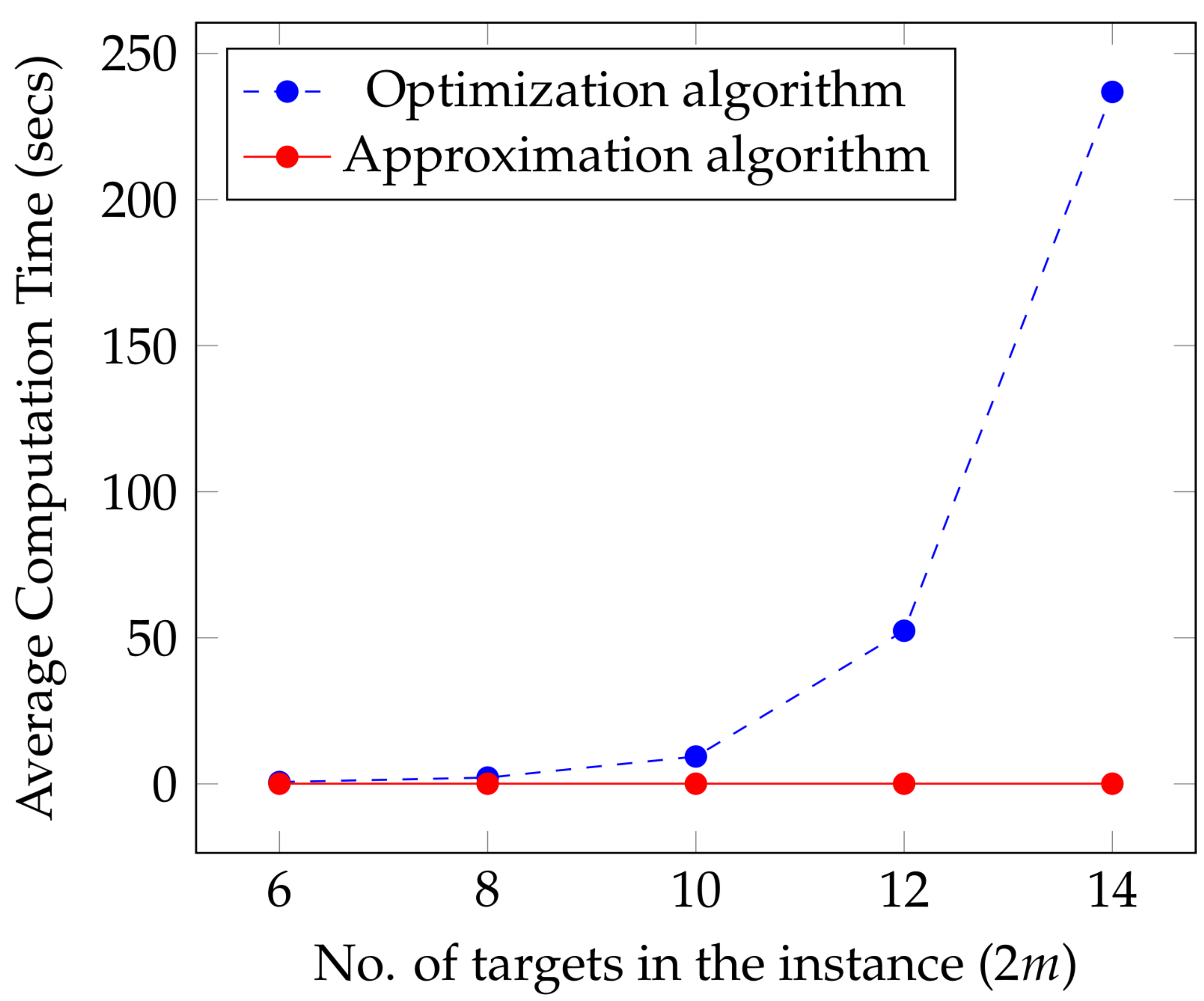
Figure 5, we plot the average computation times of the approximate and optimal solutions against the number of targets in the instance. For a given number of targets, the average is computed over 50 instances that share the same number of targets. From the figure, it can be observed that the average computation time for the approximate solutions is significantly lower than that for the optimal solutions. Additionally, while the average time for the latter increases rapidly with the number of targets in the instances, the average time for the former remains consistent across all small instances, at 0.06 s, indicating better scalability of the approximation algorithm. The average computation time for the heuristic solutions follows a similar trend as the approximate solutions. However, on average, the heuristic solutions can be computed 0.01 s faster than the approximate solutions.
The quality of the solutions provided by the approximation and heuristic algorithms and the significant savings in the computation time offered by these algorithms suggest that they can be used as an alternative to computing optimal solutions, especially in large instances where either the optimal solutions are unavailable or good-quality solutions need to be computed quickly.
6.2. Large Instances
The number of targets in these instances ranges from 20 to 100. Due to the size of these instances, optimal solutions were not computable within the 3-h cut-off time. For every large instance, we compute the approximate and heuristic solutions and determine the ratios of the costs of these solutions to the lower bounds. The average ratios and the average computation times for both the algorithms are presented in
Table 3.
The results suggest that the average ratios for both the algorithms increase with the number of targets in the instance. Nonetheless, similar to the trend observed in small instances, the rate of increase is smaller for the heuristic algorithm compared to its counterpart. While the ratios range from 1.54 to 1.61 for the approximation algorithm, they range from 1.48 to 1.50 for the heuristic algorithm. It is to be noted that these ratios are not significantly higher than those observed in the case of small instances. Therefore, it is likely that the quality of the solutions provided by these algorithms is as good as that observed in small instances. However, this claim cannot be justified without improved lower bounds in the future.
In comparison, the average quality of the solutions provided by the heuristic algorithm was observed to be slightly better than those provided by the approximation algorithm. This can be attributed to the difference in the type of single UV tours provided by these algorithms.
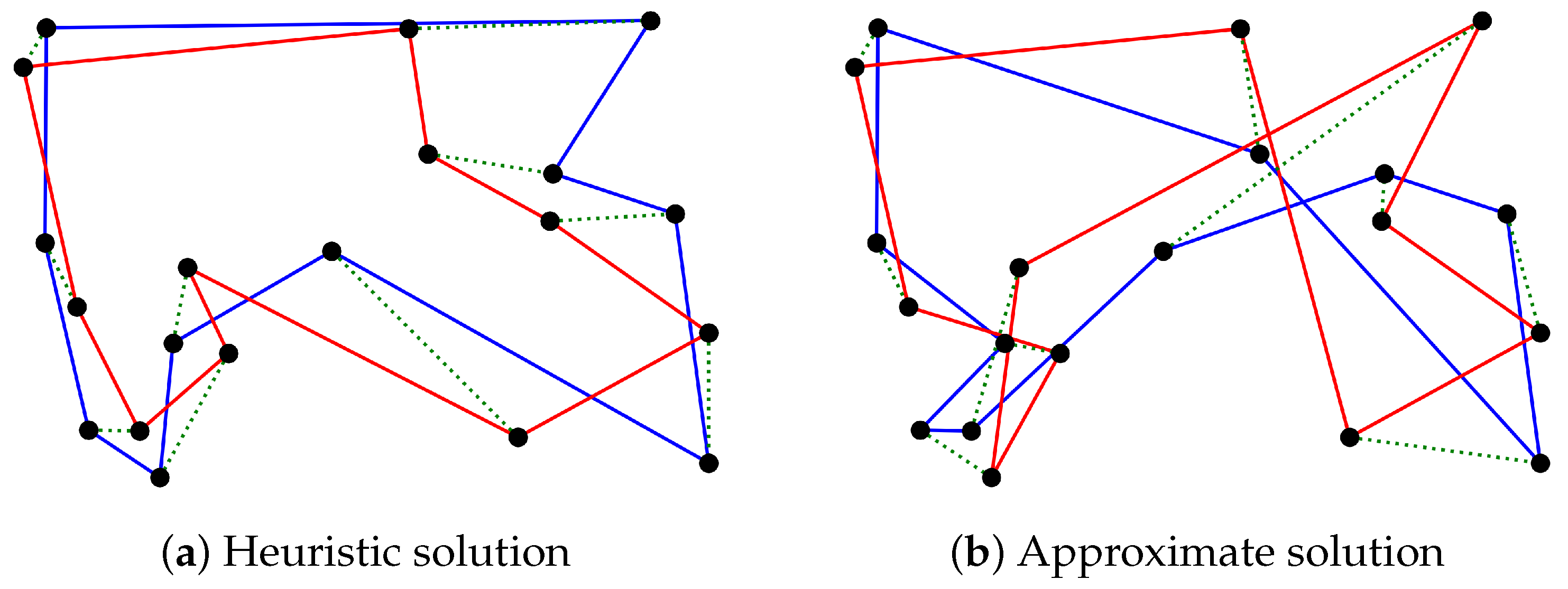
Figure 6a,b depict feasible solutions for an illustrative 20-target instance computed using the heuristic and the approximation algorithms, respectively. As can be seen from the figure, the vehicle tours provided by the latter contain criss-cross paths as opposed to those provided by the former. The presence of criss-crossing is an undesirable feature in TSP tours and contributes to higher costs.
However, the average computation time of the approximation algorithm was observed to be slightly better than that of the heuristic algorithm for large instances. Additionally, the approximation algorithm offers guarantees on the worst-case solution quality and computation time. Therefore, there is a trade-off involved in selecting the desired algorithm. Nevertheless, the computation times for both algorithms are within a fraction of a second for instances with up to 100 targets and the algorithms provide good-quality solutions based on the ratios observed in the case of small instances. Therefore, both algorithms are useful in practice, especially when optimal solutions are not computable within the desired time.
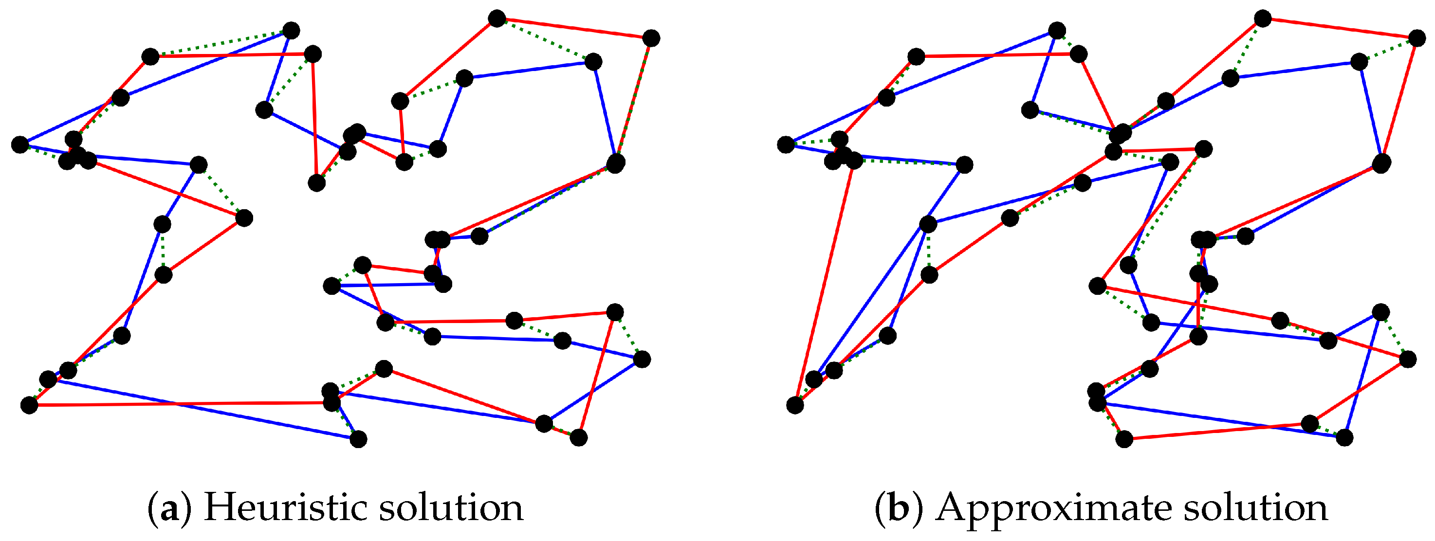
Figure 7a,b show feasible solutions computed in 0.20 and 0.08 s using the heuristic and approximation algorithms, respectively, for a 50-target instance, for which optimal solutions were not computable within 3 h.
7. Summary
In this article, we considered a problem in which a pair of unmanned vehicles are required to visit a set of targets to perform tasks therein. The vehicles are required to visit disjoint sets of targets and coordinate their visits such that they can communicate with each other after visiting every target in their sequence. The objective is to determine tours and target assignments for the UVs such that the energy consumed for traveling and communicating is minimized. We formulated this problem as an integer program and highlighted the difficulty in computing optimal solutions to large instances of the problem.
For the ease of algorithmic development, we first considered a special case of the problem in which equal weights are assigned in the objective function to the distances traveled by the vehicles and the distances between them while communicating. For this problem, we developed two algorithms, an approximation algorithm and a heuristic algorithm, to compute high-quality solutions swiftly. The approximation algorithm has a fixed a priori ratio of 3.75. To evaluate the performance of these algorithms, we performed extensive numerical experiments on 500 instances of the problem. The results of the experiments indicate that the quality of the algorithmic solutions is better in practice than its theoretical worst-case bound. The heuristic algorithm provided solutions with different structures than that of the approximate solutions. Though the heuristic solutions were observed to have a slightly better cost than the algorithmic solutions on average, neither algorithm outperformed the other on all problem instances and all performance metrics. Furthermore, both algorithms provided feasible solutions to the problem within a fraction of a second for instances with at most 100 targets on a MacBook Pro with 16 GB RAM, Quad-Core Intel Core i7 processor @ 2.8 GHz. Later, we showed that the approximation algorithm provides feasible solutions to the general weighted case, and has a variable a priori ratio of when and when .
In addition to contributing the aforementioned algorithms, in this paper, we developed lower bounds that help in evaluating the quality of feasible solutions to the problem. The gaps between the cost of the algorithmic solutions and the lower bound are similar for small- and large-scale instances. This suggests that the solution performance may not deteriorate significantly with the problem size. However, this claim cannot be justified without improving the lower bounds in the future.
In
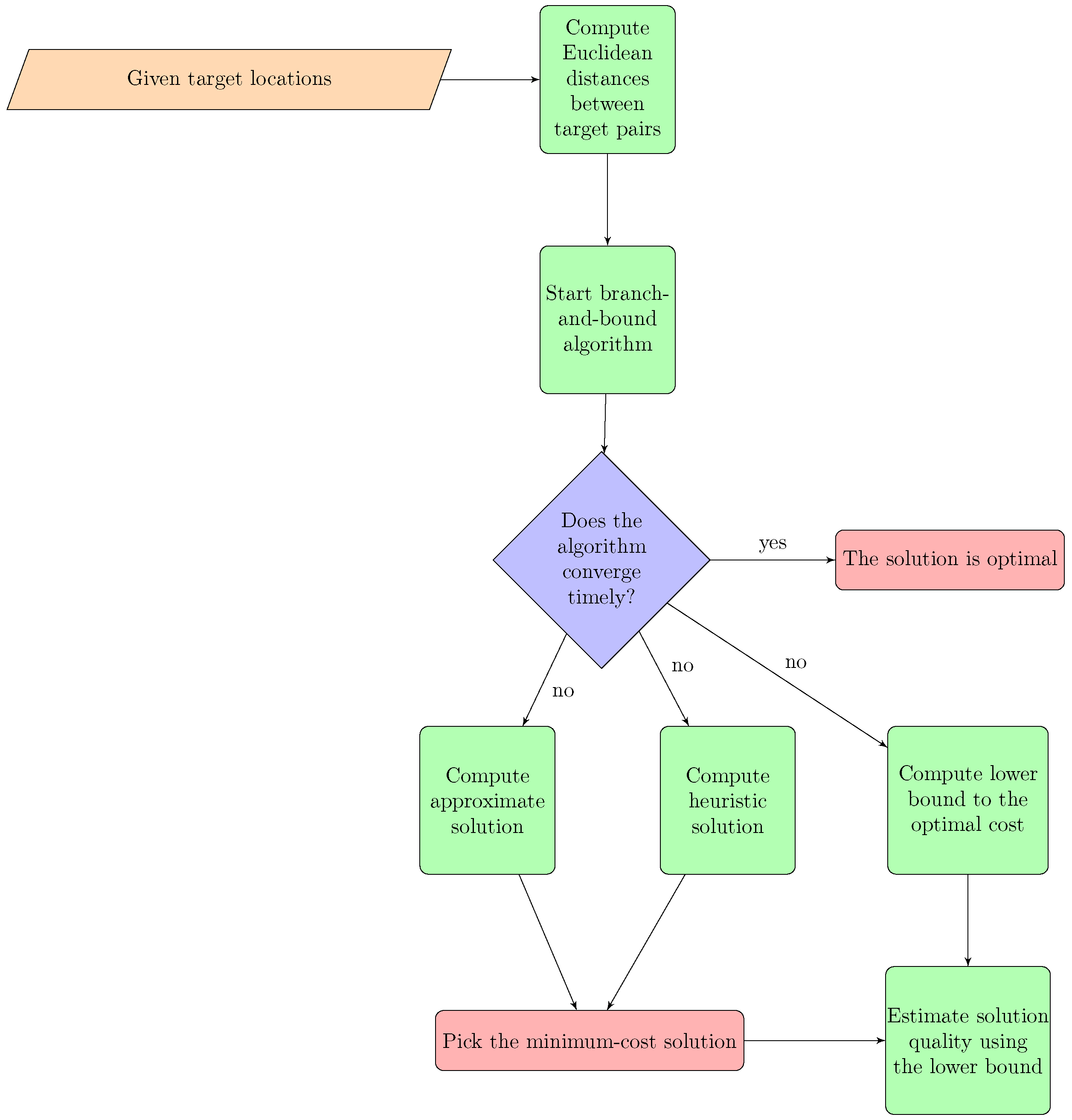
Figure 8, we summarize the workflow of the paper to improve the ease of understanding the role of the developed algorithms and lower bounds in determining feasible solutions to the problem and evaluating their quality.
Despite these contributions, the work done in this paper has a few limitations. A majority of the algorithmic development has been focused on the equally weighted case. While an approximation algorithm is available to solve the general weighted problem, its solutions have a worst-case performance that varies with the ratio of the weights. Therefore, there is a need for developing algorithms that are tailor-made to solve the weighted problem. One way to develop such tailor-made algorithms for the weighted case is to iteratively increase the weights assigned to either travel or communication costs and observe the changes in the solution structures. Additionally, the developed lower bounds for the optimal cost are not binding and there is a scope for improving these bounds. A few potential future directions to improve the lower bounds include (1) developing alternate formulations to the problem, (2) solving linear relaxations of different formulations of the problem, and (3) generating strong valid inequalities to improve the problem representation.
Author Contributions
Conceptualization, S.K.K.H., S.R., S.D. and D.C.; methodology, S.K.K.H., S.R., S.D. and D.C.; validation, S.K.K.H. and S.D.; formal analysis, S.K.K.H. and S.D.; investigation, S.K.K.H. and S.D; resources, S.K.K.H., S.R., S.D. and D.C.; data curation, S.K.K.H.; writing—original draft preparation, S.K.K.H., S.R., S.D. and D.C.; writing—review and editing, S.K.K.H., S.R., S.D. and D.C.; visualization, S.K.K.H.; supervision, S.K.K.H., S.R., S.D. and D.C.; project administration, S.K.K.H., S.R., S.D. and D.C.; funding acquisition, S.K.K.H., S.R., S.D. and D.C. All authors have read and agreed to the published version of the manuscript.
Funding
This research was funded by the Laboratory Directed Research & Development (LDRD) project “The Optimization of Machine Learning: Imposing Requirements on Artificial Intelligence” of the Los Alamos National Laboratory. This article has been approved for public Release; Distribution is Unlimited. PA# AFRL-2022-4269 and LA-UR-22-30345.
Data Availability Statement
Data sharing is not applicable to this article.
Conflicts of Interest
The authors declare no conflict of interest.
Appendix A. Approximation Ratio for the General Weighted Case
When the weights assigned to the travel and communication distances are not equal, i.e.,
, the approximation algorithm presented in
Section 5 still presents feasible solutions. This is because the constraints for the weighted and the unweighted case remain the same. However, we will show in this section that the approximation ratio of the algorithm for the weighted case has a variable ratio. Towards this end, let the ratio of the weights assigned to the communication and travel distances be defined as
. Then, let us consider two cases:
and
.
When
, the objective function can be equivalently scaled by assigning weights
and
, without changing the solutions and the approximation ratio. Then, from the construction of the algorithm, it follows that
This provides an upper bound on the optimal cost of the solution. Next, observe that the optimal value of the solutions to the weighted case is at least equal to that of the weighted case. That is,
. Then, it follows from inequality (
26) that the cost of the optimal solution for the weighted case is at least equal to
. As a result, when
, the algorithm has an approximation ratio of
.
When
, the objective function can be equivalently scaled by assigning weights
and
. Then, it follows from the construction of the algorithm that
Similar to the case with , here, the optimal value is lower-bounded by . Therefore, when , the algorithm has an approximation ratio of .
References
- Walambe, R.; Marathe, A.; Kotecha, K. Multiscale object detection from drone imagery using ensemble transfer learning. Drones 2021, 5, 66. [Google Scholar] [CrossRef]
- Rathinam, S.; Kim, Z.W.; Sengupta, R. Vision-based monitoring of locally linear structures using an unmanned aerial vehicle. J. Infrastruct. Syst. 2008, 14, 52–63. [Google Scholar] [CrossRef]
- Casbeer, D.W.; Beard, R.W.; McLain, T.W.; Li, S.M.; Mehra, R.K. Forest fire monitoring with multiple small UAVs. In Proceedings of the 2005 American Control Conference, Portland, OR, USA, 8–10 June 2005; pp. 3530–3535. [Google Scholar]
- Hari, S.K.K.; Rathinam, S.; Darbha, S.; Manyam, S.G.; Kalyanam, K.; Casbeer, D. Bounds on Optimal Revisit Times in Persistent Monitoring Missions With a Distinct and Remote Service Station. IEEE Trans. Robot. 2022, 39, 1070–1086. [Google Scholar] [CrossRef]
- Liu, Y.; Dai, H.N.; Wang, Q.; Shukla, M.K.; Imran, M. Unmanned aerial vehicle for internet of everything: Opportunities and challenges. Comput. Commun. 2020, 155, 66–83. [Google Scholar] [CrossRef]
- Muchiri, G.; Kimathi, S. A review of applications and potential applications of UAV. In Proceedings of the Sustainable Research and Innovation Conference, Pretoria, South Africa, 20–24 June 2022; pp. 280–283. [Google Scholar]
- Ren, H.; Zhao, Y.; Xiao, W.; Hu, Z. A review of UAV monitoring in mining areas: Current status and future perspectives. Int. J. Coal Sci. Technol. 2019, 6, 320–333. [Google Scholar] [CrossRef]
- Lu, X.; Wicker, F.; Lio, P.; Towsley, D. Security estimation model with directional antennas. In Proceedings of the MILCOM 2008—2008 IEEE Military Communications Conference, San Diego, CA, USA, 17–19 November 2008; pp. 1–6. [Google Scholar]
- Lu, X.; Wicker, F.D.; Towsley, D.; Xiong, Z.; Lio, P. Detection probability estimation of directional antennas and omni-directional antennas. Wirel. Pers. Commun. 2010, 55, 51–63. [Google Scholar] [CrossRef]
- Wang, H.; Cheng, H.; Hao, H. The use of unmanned aerial vehicle in military operations. In Proceedings of the 20th International Conference on Man-Machine-Environment System Engineering, Zhengzhou, China, 19–21 December 2020; pp. 939–945. [Google Scholar]
- Bektas, T. The multiple traveling salesman problem: An overview of formulations and solution procedures. Omega 2006, 34, 209–219. [Google Scholar] [CrossRef]
- França, P.M.; Gendreau, M.; Laporte, G.; Müller, F.M. The m-traveling salesman problem with minmax objective. Transp. Sci. 1995, 29, 267–275. [Google Scholar] [CrossRef]
- Montoya-Torres, J.R.; Franco, J.L.; Isaza, S.N.; Jiménez, H.F.; Herazo-Padilla, N. A literature review on the vehicle routing problem with multiple depots. Comput. Ind. Eng. 2015, 79, 115–129. [Google Scholar] [CrossRef]
- Mosteo, A.R.; Montano, L.; Lagoudakis, M.G. Multi-robot routing under limited communication range. In Proceedings of the 2008 IEEE International Conference on Robotics and Automation, Pasadena, CA, USA, 19–23 May 2008; pp. 1531–1536. [Google Scholar]
- Mosteo, A.R.; Montano, L.; Lagoudakis, M.G. Guaranteed-performance multi-robot routing under limited communication range. In Distributed Autonomous Robotic Systems 8; Springer: Berlin, Germany, 2009; pp. 491–502. [Google Scholar]
- Chopra, S.; Egerstedt, M. Multi-robot routing under connectivity constraints. IFAC Proc. Vol. 2012, 45, 67–72. [Google Scholar] [CrossRef]
- Banfi, J.; Basilico, N.; Amigoni, F. Multirobot reconnection on graphs: Problem, complexity, and algorithms. IEEE Trans. Robot. 2018, 34, 1299–1314. [Google Scholar] [CrossRef]
- Hollinger, G.; Singh, S. Multi-robot coordination with periodic connectivity. In Proceedings of the 2010 IEEE International Conference on Robotics and Automation, Anchorage, AL, USA, 3–8 May 2010; pp. 4457–4462. [Google Scholar]
- Scherer, J.; Schoellig, A.P.; Rinner, B. Min-Max Vertex Cycle Covers With Connectivity Constraints for Multi-Robot Patrolling. IEEE Robot. Autom. Lett. 2022, 7, 10152–10159. [Google Scholar] [CrossRef]
- Mei, Y.; Lu, Y.H.; Hu, Y.C.; Lee, C.G. A case study of mobile robot’s energy consumption and conservation techniques. In Proceedings of the 12th International Conference on Advanced Robotics, San Francisco, CA, USA, 12–15 October 2005; pp. 492–497. [Google Scholar]
- Ooi, C.C.; Schindelhauer, C. Minimal energy path planning for wireless robots. Mob. Netw. Appl. 2009, 14, 309–321. [Google Scholar] [CrossRef]
- Mardani, A.; Chiaberge, M.; Giaccone, P. Communication-aware UAV path planning. IEEE Access 2019, 7, 52609–52621. [Google Scholar] [CrossRef]
- Yan, Y.; Mostofi, Y. Communication and path planning strategies of a robotic coverage operation. In Proceedings of the 2013 American Control Conference, Washington, DC, USA, 17–19 June 2013; pp. 860–866. [Google Scholar]
- Ghaffarkhah, A.; Mostofi, Y. Dynamic networked coverage of time-varying environments in the presence of fading communication channels. ACM Trans. Sens. Netw. TOSN 2014, 10, 1–38. [Google Scholar] [CrossRef]
- Pferschy, U.; Staněk, R. Generating subtour elimination constraints for the TSP from pure integer solutions. Cent. Eur. J. Oper. Res. 2017, 25, 231–260. [Google Scholar] [CrossRef] [PubMed]
- Sundar, K.; Rathinam, S. Algorithms for heterogeneous, multiple depot, multiple unmanned vehicle path planning problems. J. Intell. Robot. Syst. 2017, 88, 513–526. [Google Scholar] [CrossRef]
- Bektaş, T.; Gouveia, L. Requiem for the Miller–Tucker–Zemlin subtour elimination constraints? Eur. J. Oper. Res. 2014, 236, 820–832. [Google Scholar] [CrossRef]
- Mars, S. What Is the Difference between User Cuts and Lazy Constraints? 2021. Available online: https://support.gurobi.com/hc/en-us/articles/360025804471-What-is-the-difference-between-user-cuts-and-lazy-constraints- (accessed on 28 May 2023).
- Christofides, N. Worst-Case Analysis of a New Heuristic for the Travelling Salesman Problem; Technical Report; Carnegie-Mellon Univversity Management Sciences Research Group: Pittsburgh, PA, USA, 1976. [Google Scholar]
- Galil, Z. Efficient algorithms for finding maximum matching in graphs. ACM Comput. Surv. CSUR 1986, 18, 23–38. [Google Scholar] [CrossRef]
- Lin, S.; Kernighan, B.W. An effective heuristic algorithm for the traveling-salesman problem. Oper. Res. 1973, 21, 498–516. [Google Scholar] [CrossRef]
- LKH Version 2.0.9. July 2018. Available online: http://webhotel4.ruc.dk/~keld/research/LKH/ (accessed on 28 May 2023).
- Gurobi Optimization, LLC. Gurobi Optimizer Reference Manual. 2023. Available online: https://www.gurobi.com (accessed on 28 May 2023).
Figure 1.
Figure explaining the enforcement of communication links that obey the travel sequence. Target l is the neighbor’s partner of target i if and only if l is also the partner’s neighbor of i. That is, for every pair of distinct targets, say, , there exists a target such that if and only if there exists a target such that .
Figure 2.
Figure depicts the rapid increase in the average computation time required to solve the problem with the number of targets in the instance; the average is taken over 50 instances each, for a given number of targets.
Figure 2.
Figure depicts the rapid increase in the average computation time required to solve the problem with the number of targets in the instance; the average is taken over 50 instances each, for a given number of targets.
Figure 3.
Figure illustrates the steps of the approximation algorithm using a 10-target instance. (a) Single UV tour, T, is shown in black. (b) The first UV’s tour, , is shown in blue. (c) The second UV’s tour, , is shown in red. (d) Potential sets of communication links are shown in orange and green. (e) The final solution combines , , and C (communication links in green).
Figure 4.
Figures illustrating the development of the lower bound to the problem. (a) Optimal solution, , used to illustrate the development of the lower bound. (b) Single UV tour over all the targets obtained by removing a few edges from . (c) Perfect bipartite matching formed by the remaining edges of .
Figure 5.
The figure depicts the average computation time required to solve the optimization and approximation, and algorithms in blue and red colors, respectively. The averages are computed over 50 instances each for a given number of targets.
Figure 5.
The figure depicts the average computation time required to solve the optimization and approximation, and algorithms in blue and red colors, respectively. The averages are computed over 50 instances each for a given number of targets.
Figure 6.
A feasible solution for a 20-target instance of the problem computed using the proposed heuristic and approximation algorithms. The black dots represent the target locations, the blue and red lines correspond to the 1st and 2nd vehicle tours, and the green dotted lines depict the communication links between the vehicles.
Figure 7.
A feasible solution for a 50-target instance of the problem computed using the proposed heuristic and approximation algorithms. The black dots represent the target locations, the blue and red lines correspond to the 1st and 2nd vehicle tours, and the green dotted lines depict the communication links between the vehicles.
Figure 8.
Flowchart describing the role of the algorithms and the lower bounds developed in this paper.
Figure 8.
Flowchart describing the role of the algorithms and the lower bounds developed in this paper.
Table 1.
This table presents the results of numerical simulations performed over 25 of the 250 small instances. Here, the words a posteriori and lower bound are abbreviated as Apos. and L.B., respectively, in the interest of space. Note that the presented values are not the average values, unlike the results presented in other tables.
| Instance # | # Targets | Optimal | Approximation Algorithm | Heuristic Algorithm | L.B. |
|---|
| Value | Runtime | Value | Apos. Ratio | Runtime | Ratio w.r.t. L.B. | Value | Apos. Ratio | Runtime | Ratio w.r.t. L.B. |
|---|
| 1 | 6 | 2019.58 | 0.58 | 2136.34 | 1.06 | 0.06 | 1.58 | 2140.62 | 1.06 | 0.05 | 1.59 | 1349.28 |
| 2 | 6 | 2320.60 | 0.60 | 2631.67 | 1.13 | 0.06 | 1.39 | 2631.67 | 1.13 | 0.06 | 1.39 | 1891.15 |
| 3 | 6 | 2340.35 | 0.59 | 2659.39 | 1.14 | 0.05 | 1.60 | 2994.48 | 1.28 | 0.06 | 1.8 | 1662.7 |
| 4 | 6 | 1834.62 | 0.68 | 2081.49 | 1.13 | 0.06 | 1.37 | 2162.55 | 1.18 | 0.06 | 1.43 | 1515.15 |
| 5 | 6 | 2375.09 | 0.69 | 2460.01 | 1.04 | 0.05 | 1.24 | 2507.83 | 1.06 | 0.06 | 1.26 | 1988.36 |
| 6 | 8 | 2138.56 | 2.31 | 2289.06 | 1.07 | 0.06 | 1.60 | 2284.58 | 1.07 | 0.05 | 1.60 | 1427.70 |
| 7 | 8 | 2934.60 | 2.27 | 3061.62 | 1.04 | 0.06 | 1.52 | 3061.62 | 1.04 | 0.06 | 1.52 | 2010.33 |
| 8 | 8 | 2394.92 | 1.86 | 2626.79 | 1.10 | 0.05 | 1.32 | 2508.0 | 1.05 | 0.06 | 1.26 | 1986.35 |
| 9 | 8 | 2768.99 | 2.08 | 2955.76 | 1.07 | 0.05 | 1.46 | 2955.76 | 1.07 | 0.06 | 1.46 | 2018.16 |
| 10 | 8 | 2535.43 | 2.33 | 2584.59 | 1.02 | 0.06 | 1.48 | 2584.59 | 1.02 | 0.06 | 1.48 | 1746.54 |
| 11 | 10 | 2543.27 | 11.43 | 2598.69 | 1.02 | 0.06 | 1.51 | 2598.69 | 1.02 | 0.06 | 1.51 | 1724.94 |
| 12 | 10 | 2935.21 | 8.50 | 3357.22 | 1.14 | 0.06 | 1.61 | 3038.09 | 1.04 | 0.06 | 1.46 | 2084.44 |
| 13 | 10 | 2535.19 | 7.61 | 2641.20 | 1.04 | 0.06 | 1.48 | 2641.2 | 1.04 | 0.06 | 1.48 | 1782.02 |
| 14 | 10 | 3094.96 | 13.24 | 3236.95 | 1.05 | 0.06 | 1.45 | 3182.03 | 1.03 | 0.13 | 1.42 | 2233.05 |
| 15 | 10 | 3073.28 | 8.23 | 3149.87 | 1.02 | 0.06 | 1.54 | 3149.87 | 1.02 | 0.05 | 1.54 | 2041.04 |
| 16 | 12 | 3358.94 | 63.02 | 3404.75 | 1.01 | 0.06 | 1.59 | 3404.75 | 1.01 | 0.06 | 1.59 | 2143.79 |
| 17 | 12 | 3209.36 | 25.09 | 3492.69 | 1.09 | 0.06 | 1.44 | 3422.02 | 1.07 | 0.06 | 1.41 | 2430.32 |
| 18 | 12 | 3019.62 | 40.89 | 3168.65 | 1.05 | 0.06 | 1.44 | 3168.65 | 1.05 | 0.06 | 1.44 | 2198.50 |
| 19 | 12 | 3048.37 | 82.02 | 3387.42 | 1.11 | 0.06 | 1.55 | 3197.42 | 1.05 | 0.06 | 1.46 | 2190.26 |
| 20 | 12 | 2632.85 | 35.60 | 2850.74 | 1.08 | 0.06 | 1.45 | 2867.6 | 1.09 | 0.06 | 1.46 | 1962.80 |
| 21 | 14 | 3162.88 | 227.96 | 3238.05 | 1.02 | 0.06 | 1.51 | 3238.05 | 1.02 | 0.06 | 1.51 | 2142.37 |
| 22 | 14 | 3261.45 | 410.44 | 4058.65 | 1.24 | 0.06 | 1.82 | 3419.32 | 1.05 | 0.06 | 1.54 | 2225.74 |
| 23 | 14 | 3550.04 | 152.61 | 4112.20 | 1.16 | 0.06 | 1.45 | 3742.91 | 1.05 | 0.06 | 1.32 | 2828.44 |
| 24 | 14 | 3210.55 | 171.60 | 3522.19 | 1.10 | 0.06 | 1.45 | 3402.58 | 1.06 | 0.06 | 1.4 | 2428.94 |
| 25 | 14 | 3136.03 | 120.96 | 3774.31 | 1.20 | 0.06 | 1.60 | 3245.69 | 1.03 | 0.06 | 1.38 | 2356.58 |
Table 2.
The table summarizes the quality of the solutions obtained using the approximation and heuristic algorithms for small instances of the problem. The six columns presented in the table indicate the number of targets in the instances, the a priori ratio of the approximation algorithm, the average a posteriori ratios of the approximation and the heuristic algorithms, and the average ratios of the algorithmic costs with the lower bound for the approximation and heuristic algorithms, respectively. All the averages are taken over (50) instances with the same number of targets.
| # Targets | A Priori Ratio
(Approx. Algo.) | Avg. A Posteriori Ratio | Avg. Ratio w.r.t. L.B. |
|---|
| Approx. Algo. | Heur. Algo. | Approx. Algo. | Heur. Algo. |
|---|
| 6 | 3.75 | 1.12 | 1.13 | 1.39 | 1.40 |
| 8 | 3.75 | 1.05 | 1.05 | 1.44 | 1.43 |
| 10 | 3.75 | 1.07 | 1.05 | 1.47 | 1.44 |
| 12 | 3.75 | 1.08 | 1.05 | 1.49 | 1.45 |
| 14 | 3.75 | 1.11 | 1.06 | 1.55 | 1.44 |
Table 3.
This table summarizes the results of the simulations performed over the 250 large instances of the problem. The five columns of the table indicate the number of targets in the instances, the average ratio of the cost of the algorithmic solution to the lower bound and the average computation time (runtime) for the approximation algorithm, followed by the corresponding values of the heuristic algorithm. The averages are taken over (50) instances with identical number of targets.
| # Targets | Approximation Algorithm | Heuristic Algorithm |
|---|
| Avg. Ratio w.r.t. L.B. | Avg. Runtime (s) | Avg. Ratio w.r.t. L.B. | Avg. Runtime (s) |
|---|
| 20 | 1.54 | 0.06 | 1.48 | 0.06 |
| 30 | 1.57 | 0.07 | 1.48 | 0.08 |
| 40 | 1.59 | 0.08 | 1.49 | 0.15 |
| 50 | 1.59 | 0.09 | 1.49 | 0.21 |
| 100 | 1.61 | 0.27 | 1.50 | 0.89 |
| Disclaimer/Publisher’s Note: The statements, opinions and data contained in all publications are solely those of the individual author(s) and contributor(s) and not of MDPI and/or the editor(s). MDPI and/or the editor(s) disclaim responsibility for any injury to people or property resulting from any ideas, methods, instructions or products referred to in the content. |
© 2023 by the authors. Licensee MDPI, Basel, Switzerland. This article is an open access article distributed under the terms and conditions of the Creative Commons Attribution (CC BY) license (https://creativecommons.org/licenses/by/4.0/).


