Trust–Region Nonlinear Optimization Algorithm for Orientation Estimator and Visual Measurement of Inertial–Magnetic Sensor

Abstract

This paper proposes a novel robust orientation estimator to enhance the accuracy and robustness of orientation estimation for inertial–magnetic sensors of the small consumer–grade drones. The proposed estimator utilizes a trust–region strategy within a nonlinear optimization framework, transforming the orientation fusion problem into a nonlinear optimization problem based on the maximum likelihood principle. The proposed estimator employs a trust–region Dogleg gradient descent strategy to optimize orientation precision and incorporates a Huber robust kernel to minimize interference caused by acceleration during the maneuvering process of the drone. In addition, a novel method for evaluating the performance of orientation estimators is also presented based on visuals. The proposed method consists of two parts: offline calibration of the basic cube using Augmented Reality University of Cordoba (ArUco) markers and online orientation measurement of the sensor carrier using a nonlinear optimization solver. The proposed measurement method’s accuracy and the proposed estimator’s performance are evaluated under low–dynamic (rotation) and high–dynamic (shake) conditions in the experiment. The experimental findings indicate that the proposed measurement method obtains an average re–projection error of less than 0.1 pixels. The proposed estimator has the lowest average orientation error compared to conventional orientation estimation algorithms. Despite the time–consuming nature of the proposed estimator, it exhibits greater robustness and precision, particularly in highly dynamic environments.

1. Introduction

The accuracy of orientation estimation plays a crucial role in enhancing the overall performance of drones. Numerous drone applications can benefit from accurate orientation estimation, including navigation, perception, autonomous flight, and task execution [1,2,3,4,5,6]. Firstly, improving the orientation precision in navigation applications can reduce the likelihood of unintended route deviation and ensure maritime safety in dynamic environments. Secondly, using predicted orientation information from motion sensors can mitigate the deficiencies of motion distortion in the perception system of visual detectors equipped with low–altitude drones. This characteristic enhances the output precision of the data fusion odometer in the perception system, allowing drones to make decisions based on precise perception data [3,4]. In addition, by increasing the accuracy of orientation estimation, drones can substantially enhance the dependability and efficiency of autonomous flight and task completion. By approaching the target direction, drones can implement tasks more precisely, resulting in safer and more efficient operations for applications such as plant protection and aerial photography [5,6]. In summary, improving the precision of orientation estimation has significant practical value.

Small consumer-grade drones commonly employ Micro Electrical System (MEMS) inertial–magnetic sensors as onboard orientation sensors. An inertial–magnetic sensor consists of a tri–axis gyroscope, a tri–axis accelerometer, and a tri–axis magnetometer. The magnetometer measures the intensity of magnetic induction. Under the condition of no interference from external magnetic fields, the measured value of the magnetic sensor is the geomagnetic vector, which is the tangent direction of the geomagnetic field in the magnetic induction line of the drone location (pointing to the north magnetic pole). Accelerometer is used to measure the specific force of the drone, which incorporates the acceleration of gravity and the acceleration of the drone’s motion. The direction of the gravity vector is perpendicular to the Earth’s surface and points toward the Earth’s center, which can be considered perpendicular to the Earth’s surface within a small range. The angular velocity of the drone is measured using gyroscopes. By measuring the geomagnetic vector, drones equipped with inertial–magnetic sensors could correct their heading without interference from an external magnetic field [7]. It is clear that the airborne inertial–magnetic sensor’s orientation fusion method offers a broader range of possible applications than the inertial measurement unit (IMU).

Two significant factors affect the orientation precision of inexpensive drones. First, the inherent limitations of the MEMS devices used in these drones, such as gyroscope drift and random drift, necessitate more precise integrated gyroscope orientation measurements. The second factor is the effect of drone maneuvering acceleration on the measurement of gravitational acceleration, which impacts the precision of orientation estimation. Using the gravity acceleration vector and geomagnetic vector to correct the orientation of drones is the central concept of current mainstream orientation estimation algorithms, which aim to circumvent the issues listed above. These algorithms can be broadly categorized into two groups. The first type of complementary filtering algorithm and its derivative methods [8,9,10,11] combine sensor data with a high signal–to–noise ratio, such as the high–frequency component of gyroscope data and the low-frequency component of other sensor (accelerometer and magnetic sensors) data, based on device characteristics. The Mahony filter [10] and Madgwick filter [11] are two typical implementations of complementary filters. The Mahony filter takes advantage of the benefits of accelerometers and gyroscopes by modifying fusion process weights using proportional and integral (PI) controllers in the frequency domain to establish a complementary relationship between gyroscope and accelerometer outputs and to reduce drift errors. For efficient quaternion updates, the Madgwick filter employs a gradient descent algorithm. It utilizes boundary conditions to determine the filter gain, ensuring that convergence speed is not less than the speed of orientation changes. This form of algorithm is frequently utilized in tiny consumer drones. The second group consists of algorithms that employ Kalman filters [12,13,14,15], such as the extended Kalman filter (EKF) [12] and error–state Kalman filter (ESKF) [13,14,15]. These algorithms use sensor covariance–based measurement data combinations to recursively rectify and reduce the orientation estimator’s variance, enhancing its accuracy. The Kalman filter is optimal for linear systems with minimal variance and relies on precise prior sensor parameter knowledge. Inaccurate filtering parameters can lead to convergence on incorrect solutions, thereby causing inconsistency [14]. Compared to the nominal variable, the ESKF state variable is an error quantity, which is a minor quantity that changes slowly. Utilizing error variables permits filters to linearize the ideal model more precisely.

To enhance the precision and robustness of orientation estimation, we propose a novel estimator based on a nonlinear optimization framework that is inspired by the Madgwick filter and ESKF. Three stages make up the proposed algorithm. From the quaternion kinematics equation, we first derive an a priori solution for the orientation variable. Next, we derive an optimization problem for the increment of orientation variables based on the principle of maximum likelihood. The trust–region solver is then used to update the orientation quaternion. We incorporate Huber robust kernel functions into the solver to reduce the effect of maneuvering acceleration on measurements of gravity.

We also propose a method for measuring orientation using a monocular camera to evaluate the precision performance of the estimator. The proposed measurement method consists of two stages: the offline calibration of the Base Cube (where the sensor is attached to a Base Cube Augmented Reality University of Cordoba (ArUco) [16,17] marker–labeled) and the online measurement of sensor orientation. During the calibration procedure, we generate multiple data pairings using the Perspective–n–Point (PnP) [18] algorithm and combine them with a nonlinear optimization solver to determine the relative rotation relationship between adjacent markers. We also measure the relative rotation of the Base Cube frame to the sensor body frame, which is used for orientation alignment when evaluating the estimator’s performance. We use the calibration parameters during the measurement phase to directly measure the sensor’s orientation with the PnP algorithm to increase measurement efficacy.

In the experimental portion, four experiments are conducted to assess the precision of visual measurement and the performance of the orientation estimator: PnP algorithm accuracy testing, adjacent marker calibration accuracy testing, hand–eye calibration accuracy testing, and estimator performance testing. According to the test results, the ArUco–based orientation estimation is highly accurate, and all the combined algorithms that participated in the test achieve positive results. The P3P algorithm combined with the Dogleg optimizer obtains the lowest rotation error in all five test sets. The utmost attitude residual after alignment, as determined by the hand–eye calibration results, is 0.044 rad. Using the measured reference orientation, the performance of complementary filters (Mahony [10] and Madgwick [11]) and ESKF on the Advanced ARM Machine (ARM) platform, as well as the performance of the proposed estimator, are evaluated. The proposed algorithm displays a small average orientation error (absolute value) under low– and high–dynamic conditions. Under highly dynamic conditions, the performance advantage of the proposed algorithm is particularly evident, indicating that it is more resistant to the interference of maneuvering acceleration.

As a supplement, we assess the estimator’s efficiency on the ARM and X86–64 platforms. According to the experimental findings, the Madgwick filter [11] has the quickest calculation speed for orientation. The average runtime of the proposed estimator for a single frame on the ARM platform is 22.4 ms, while on the X86-64 platform, it is 2.67 ms. Although it is time–consuming, the proposed algorithm can calculate orientation in real–time and is more accurate and robust than traditional algorithms.

The main contributions of this paper are as follows:

1.

We propose a novel nonlinear optimization algorithm for improving the bearing estimation of inexpensive airborne inertial–magnetic sensors. The proposed algorithm utilizes the Huber robust kernel to suppress maneuvering acceleration interference of the drone and a trust-region strategy to optimize positioning precision. The experiments indicate that our algorithm has significant advantages in orientation accuracy under high–dynamic conditions.

2.

We propose a method for measuring orientation with a monocular camera based on nonlinear optimization and evaluate the measurement error of the proposed method in depth.

3.

We evaluate the accuracy and robustness of the proposed estimator, complementary filtering algorithms, and typical implementations of Kalman filtering algorithms relative to visual reference orientation under low– and high–dynamic conditions on the ARM platform. In addition, we assess the operational effectiveness of the aforementioned algorithms on the X86–64 and ARM platforms, which can serve as a reference for airborne multimodal fusion units.

2. Related Work

2.1. Trust–Region Optimization Algorithm

As a solver for nonlinear optimization problems, the trust–region algorithm has widespread application in multi–sensor fusion and visual localization. The nonlinear optimization framework has demonstrated higher accuracy in sensor fusion localization [19,20] compared to KF algorithms due to optimization algorithms’ capability to iteratively improve the precision of optimization variables throughout the process. The primary objective of the trust–region algorithm is to solve the cost function within a bounded region by choosing an appropriate step size for each iteration. The Levenberg–Marquardt (LM) algorithm and Dogleg algorithm are typical trust–region algorithm implementations [21]. The gradient descent strategy is the primary difference between the two algorithms. The LM algorithm accomplishes optimization by balancing the step size of the local model and the quality (descent ratio) by adjusting the damping factor. The damping factor is introduced in the LM algorithm to guarantee the positive definiteness of the Hessian matrix, thereby ensuring that the iteration is always in the direction of decreasing the loss function value. The Dogleg algorithm calculates Gaussian–Newton and gradient descent steps independently during each iteration step and chooses the updated trajectory and step size based on the trust zone radius. For small–scale optimization problems, the Dogleg algorithm usually has a faster convergence speed compared to the LM algorithm [22]. In order to enhance the accuracy of orientation estimation and measurement, we draw inspiration from the nonlinear optimization framework and employ the trust-region algorithm as a solver. We aim to optimize the estimation process and refine the measurements by leveraging the trust-region algorithm.

2.2. Perspective–n–Point Algorithm

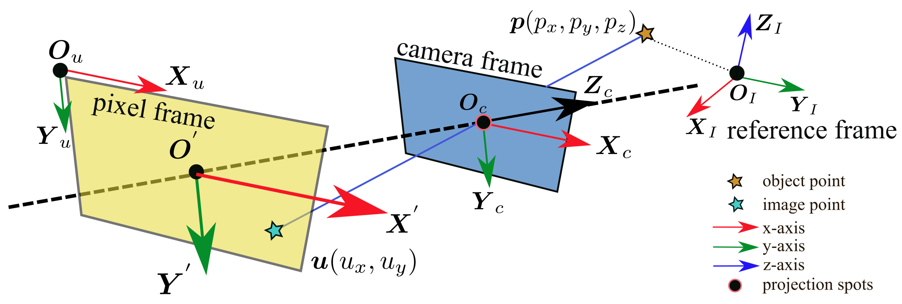
A fundamental task in visual orientation measurement is to recover the camera’s pose relative to a reference frame using a camera projection model. This involves associating image coordinates with corresponding points in the real world, allowing for the estimation of the camera’s pose. Typically, the Perspective–n–Point (PnP) algorithm is utilized for this purpose, as it attempts to precisely compute the camera’s position and orientation based on the correspondence between 3D reference points and their 2D image projections. By employing the PnP algorithm, we can effectively recover the camera’s pose from visual measurements and align it to the reference coordinate system. The Perspective–n–Point (PnP) algorithm [19] is a class of camera orientation estimation algorithms. It computes the camera’s position and orientation based on its projection model, using known 3D points and their image projection points. Practical applications of the PnP algorithm include robot navigation, augmented reality, autonomous transportation, and 3D reconstruction. As illustrated in Figure 1, the input of the PnP algorithm are the object points in the reference frame and their corresponding image points in the camera normalized camera coordinate system. The output are the camera’s rotation and translation matrices. Standard PnP algorithm implementations include Perspective-3-Point (P3P) [23,24,25], direct linear transform (DLT) [26], EPnP [27], and UPnP [28]. The P3P algorithm solves the rotation and translation matrices of the camera based on the geometric relationship between object points and image points. The DLT algorithm solves the PnP problem using linear equations. The EPnP algorithm is a nonlinear optimization–based algorithm that solves the rotation and translation matrices of the camera by minimizing the re–projection error in the camera frame. The UPnP algorithm is also a nonlinear optimization based algorithm. Unlike the EPnP algorithm, the UPnP algorithm augments its optimization variables with internal camera parameters. In this paper, we endeavor to measure the orientation of the proposed estimator using a monocular camera. Due to the sensitivity of the optimization algorithm to the initial value, we use the PnP algorithm to measure the orientation as the initial value and a nonlinear optimization solver to enhance the accuracy of the attitude measurement.

2.3. ArUco Marker

The Augmented Reality University of Cordoba (ArUco) marker is a form of landmark based on two–dimensional codes (as depicted in Figure 2) that is widely used in robot pose estimation and augmented reality [29,30]. Each ArUco marker has a unique identifier (ID), and the position and posture of the markers can be determined by distinguishing the black and white squares within the ArUco marker, as well as their spatial relationships and labeling rules [31]. The ArUco marker’s recognition process begins with preprocessing operations, such as denoising and graying, to enhance the efficacy of subsequent processing. The designated edges are then extracted using edge detection algorithms, such as the Canny operator. The intersection sites on the edge are then identified, and the binary encoding of the markers is converted into identifiers by the marking rules. The ArUco marker is highly durable and adaptable to different illumination and noise environments [32]. In order to guarantee the precision of orientation assessment, we employ the ArUco marker as a visual reference in this paper.

3. Overview of Proposed Algorithm

As depicted in Figure 3, we propose an orientation estimator based on a nonlinear optimization framework and a vision-based measurement method of sensor orientation. The proposed estimator continues to rectify the orientation of the sensor using the gravity acceleration vector and geomagnetic vector. To improve the orientation accuracy, we endeavor to decouple the iterative process of solving the orientation problem from the timeline and seek the optimal solution for the orientation at each time step. Based on this concept, we transform the orientation estimation problem into a maximum likelihood based nonlinear optimization problem. Since the optimization problem is sensitive to the initial value, we estimate the orientation by solving the quaternion kinematics equation a priori. Then, we use the likelihood model of the gravity vector and magnetic vector to construct the cost function and the trust–region solver to optimize the orientation so that the iterative process is always in the orientation of gradient decline, thereby enhancing the optimization efficiency. Since the accelerometer’s measured value is the specific force of the carrier, it incorporates the carrier’s maneuvering acceleration. We implement Huber robust kernels [33] in the solver to adaptively suppress the anomalous interference of these measurements on orientation updates, enhancing the estimator’s robustness under conditions of high dynamicity.

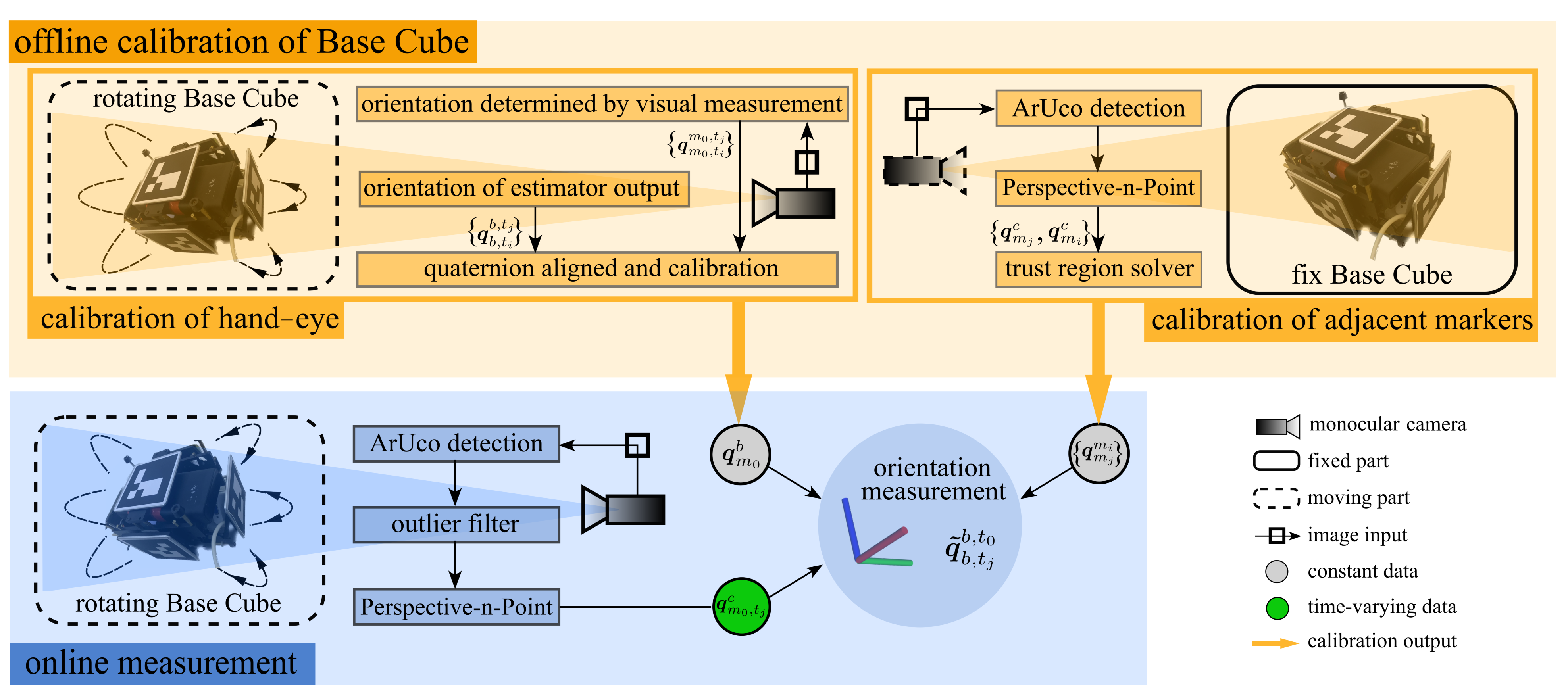
To evaluate the efficacy of the proposed orientation fusion algorithm, we also propose a method for measuring orientation using a monocular camera. Two components comprise the proposed method: offline calibration of the Base Cube and online measurement. We connect the sensor to the Base Cube and position ArUco markers with distinct patterns on each cube’s six surfaces. The objective of the offline calibration section is, therefore, to precisely measure the relative rotation of the adjacent markers and the relative rotation of the Base Cube frame concerning the sensor frame (hand–eye calibration). The former is intended to harmonize the measurement reference during the rotation process, while the latter is intended to align the orientation when evaluating the estimator’s performance. In the online measurement phase, we use the PnP algorithm directly to determine the orientation of the Base Cube based on the calibrated parameters and to align it to the sensor frame at the onset.

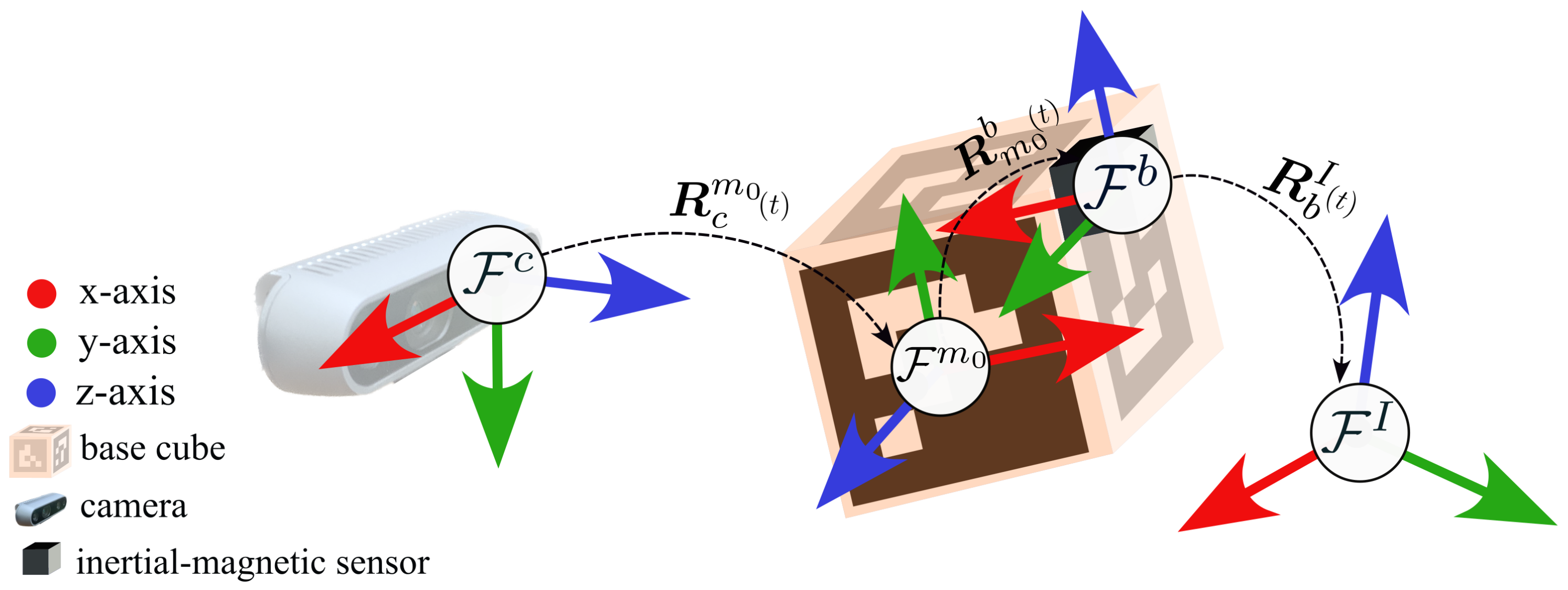
Four frames are defined to facilitate the expression of the proposed algorithm, as shown in Figure 4. We use the East-North-Upper (ENU) inertial frame, where the sensor is located at the initial time $t_0$, as the inertial reference frame ${\mathcal{F}}^I$. ${\mathcal{F}}^b$ represents the sensor body frame, whereas we use the device frame of the gyroscope. The accelerometer and magnetic part of measurement data will be projected onto ${\mathcal{F}}^b$. ${\mathcal{F}}^{m_0}$ represents the BC frame, which is also the marker frame of ID(0). In addition, we use ${\mathcal{F}}^{m_i}$ to denote the marker frame of ID(i). Each ArUco marker’s frame is unique, and the z-axis is perpendicular to the marker’s external orientation. ${\mathcal{F}}^c$ represents the spatial camera frame of the measuring camera. The z-axis is the optical center pointing outward along the camera’s optical axis, the x-axis is to the right, and the y-axis is downward.

In addition,

Table 1. The declarations of symbols and rules.

Symbols	Description
$\mathit{X}$	Bold capital letters represent matrices
$\mathit{x}$	Bold lowercase letters represent vectors
x	Scalar
$\tilde{\mathit{x}}$	Measurement value of sensor
$\breve{p}$	Probability
$\mathit{q}$	Normalized quaternion
${\left[\mathit{q}\right]}_{im}$	The imaginary part of a quaternion
${\mathit{x}}^{\circ }$	Optimal value
$\mathcal{F}$	Coordinate system

The above rules do not apply to table headers.

displays the symbols and rules we used in this paper.

4. Proposed Robust Orientation Estimator

This section introduces three components of the robust orientation estimator in depth: the quaternion kinematic, the cost function of field measurement, and the robust trust–region solver.

4.1. Quaternion Kinematic

The Hamiltonian quaternion $\mathit{q}$ is used as this paper’s parameterized form of the orientation variable. The Hamiltonian quaternion can be represented as:

$$\left\{{\mathit{q}|\mathit{q}=[w,\mathit{v}]}^T,w\in \mathbb{R},\mathit{v}\in {\mathbb{R}}^3\right\}$$

(1)

If ${\mathit{q}}_b^I\left(t\right)$ is the sensor body frame ${\mathcal{F}}^b$ relative inertial reference system ${\mathcal{F}}^I$ orientation quaternion, then the quaternion kinematic is as follows:

$${\dot{\mathit{q}}}_{\mathit{b}}^{\mathit{I}}\left(t\right)=\frac{1}{2}\mathbf{\Omega }\left({\omega }^b\left(t\right)\right){\mathit{q}}_b^I\left(t\right)$$

(2)

$$\mathbf{\Omega }\left({\omega }_b\right)=\left[\begin{array}{cc}0& -{\omega }_{\mathit{b}}^T\\ {\omega }_{\mathit{b}}& -{\omega }_b^{\wedge }\end{array}\right],{\omega }_b^{\wedge }=\left[\begin{array}{ccc}0& -{\omega }_{bz}& {\omega }_{by}\\ {\omega }_{bz}& 0& -{\omega }_{bx}\\ -{\omega }_{by}& {\omega }_{bx}& 0\end{array}\right]$$

(3)

where ${\omega }_b={\left[{\omega }_{bx}{\omega }_{by}{\omega }_{bz}\right]}^T$ represents the angular velocity of body frame ${\mathcal{F}}^b$. To derive the quaternion ${\mathit{q}}_{b,k}^I$ at time k, we digitally discretize Equation (2). The $k+1$ time interval $\Delta t$ orientation quaternion ${\mathit{q}}_{b,k+1}^I$ derived by median integration is:

$${\mathit{q}}_{b,k+1}^I={\mathit{q}}_{b,k}^I+\frac{1}{2}({\dot{\mathit{q}}}_{b,k}^I+{\dot{\mathit{q}}}_{b,k+1}^I)\Delta t$$

(4)

4.2. Cost Function of Field Measurement

The field vectors (gravity vector and magnetic vector) at the sensor location can be approximated as constant vectors in ${\mathbb{R}}^3$ in a narrow range. In theory, using field vectors in two separate coordinate systems can restore relative rotation between coordinate systems. An accelerometer’s measured value is the specific force, which incorporates gravity and the carrier’s maneuvering acceleration. Because of the interference of carrier maneuvering acceleration, the precision of the observed value of gravity acceleration is unclear. Thus, we model the uncertainty of carrier maneuvering acceleration as the noise term ${\eta }_a\in {\mathbb{R}}^3$ and obtain the measurement model as follows:

$${\tilde{\mathit{a}}}_k={[{\left({\mathit{q}}_{b,k}^I\right)}^{*}\otimes \mathit{q}\left({\mathit{g}}^I\right)\otimes {\mathit{q}}_{b,k}^I]}_{im}+{\eta }_a$$

(5)

$$\mathit{q}\left({\tilde{\mathit{a}}}_k\right)={\left[0{\tilde{\mathit{a}}}_k\right]}^T$$

(6)

where ${\tilde{\mathit{a}}}_k\in {\mathbb{R}}^3$ is the accelerometer measurement value at time k. ${\left({\mathit{q}}_{b,k}^I\right)}^{*}$ is the conjugation of the quaternion ${\mathit{q}}_{b,k}^I$. The gravity vector in ${\mathcal{F}}^I$ is denoted by ${\mathit{g}}^I$. The imaginary component of the quaternion $\mathit{q}$ is represented by ${\left[\mathit{q}\right]}_{im}$. Assume that ${\eta }_a\sim \mathcal{N}({\mathbf{0}}_{3\times 1},{\sigma }_a)$, while ${\sigma }_a\in {\mathbb{R}}^3$ is the gravity measurement variance. Then, we obtain the likelihood probability of the gravity measurement, which is:

$$\breve{p}\left({\tilde{\mathit{a}}}_{\mathit{k}}\right|{\mathit{q}}_{b,k}^I)={\lambda }_{a}exp\frac{1}{2}\left({\mathit{e}}_{a,k}{({\mathit{q}}_{b,k}^I,{\tilde{\mathit{a}}}_k)}^T{\mathbf{\Sigma }}_a^{-1}{\mathit{e}}_{a,k}({\mathit{q}}_{b,k}^I,{\tilde{\mathit{a}}}_k)\right)$$

(7)

$${\mathit{e}}_{a,k}({\mathit{q}}_{b,k}^I,{\tilde{\mathit{a}}}_k)={[{\left({\mathit{q}}_{b,k}^I\right)}^{*}\otimes \mathit{q}\left({\mathit{g}}^I\right)\otimes {\mathit{q}}_{b,k}^I]}_{im}-{\tilde{\mathit{a}}}_k$$

(8)

where ${\lambda }_a$ is a constant that is independent of ${\mathit{q}}_{b,k}^I$. ${\mathit{g}}^I$ is the gravity in reference frame ${\mathcal{F}}^I$. The cost function of the measured gravity at time k is defined as ${\mathit{e}}_{a,k}({\mathit{q}}_{b,k}^I,{\tilde{\mathit{a}}}_k)\in {\mathbb{R}}^3$.

Given that a vector’s rotation in ${\mathbb{R}}^3$ remains constant at any angle around itself, a single field vector cannot uniquely correspond to the orientation of the relative inertial reference frame. The quaternion determined by Equation (5) can only spin the sensor to the horizontal plane and cannot uniquely calculate the heading angle. In order to construct the measurement model of the magnetic vector, we, therefore, employ the strategy of the Madgwick filter [9], which opts for a fixed heading angle. Assuming that the magnetometer’s measured values only include the geomagnetic vector. As depicted in Figure 5, initially, it can be seen that the geomagnetic vector ${\tilde{\mathit{m}}}_{\mathit{b},\mathit{k}}$ measured by the sensor at time k is transformed into the inertial reference frame ${\mathcal{F}}^I$ using the quaternion determined by gravity vector to obtain ${\check{\mathit{m}}}_{\mathit{I},\mathit{k}}$. Next, ${\check{\mathit{m}}}_{\mathit{I},\mathit{k}}$ is rotated around the z–axis of ${\mathcal{F}}^I$ to obtain ${\widehat{\mathit{m}}}_{\mathit{I},\mathit{k}}$ in the YOZ plane. Based on the preceding analysis, the following measurement model for the geomagnetic vector can be derived:

$${\check{\mathit{m}}}_{\mathit{I},\mathit{k}}=\left[\begin{array}{c}{\check{m}}_{I,k}^x\\ {\check{m}}_{I,k}^y\\ {\check{m}}_{I,k}^z\end{array}\right]=\mathit{R}\left({\mathit{q}}_{b,k}^I\right){\tilde{\mathit{m}}}_{\mathit{b},\mathit{k}}+{\eta }_m$$

(9)

$$\mathit{R}\left({\mathit{q}}_{b,k}^I\right)=\left[\begin{array}{ccc}1-2q_y^2-q_z^2& 2(q_x{q}_y-q_w{q}_z)& 2(q_x{q}_z+q_w{q}_y)\\ 2(q_x{q}_y+q_w{q}_z)& 1-2q_x^2-q_z^2& 2(q_y{q}_z-q_w{q}_x)\\ 2(q_x{q}_z-q_w{q}_y)& 2(q_y{q}_z+q_w{q}_x)& 1-2q_x^2-q_y^2\end{array}\right]$$

(10)

where ${\eta }_m\sim \mathcal{N}({\mathbf{0}}_{3\times 1},{\sigma }_m)$ is the noise term of geomagnetic measurement. The following can be deduced from the geometric relationship between ${\check{\mathit{m}}}_{\mathit{I},\mathit{k}}$ and ${\widehat{\mathit{m}}}_{\mathit{I},\mathit{k}}$:

$${\widehat{\mathit{m}}}_{\mathit{I},\mathit{k}}=\left[\begin{array}{c}{\widehat{m}}_{I,k}^x\\ {\widehat{m}}_{I,k}^y\\ {\widehat{m}}_{I,k}^z\end{array}\right]=\left[\begin{array}{c}\sqrt{{\left({\check{m}}_{I,k}^x\right)}^2+{\left({\check{m}}_{I,k}^y\right)}^2}\\ 0\\ {\check{m}}_{I,k}^z\end{array}\right]$$

(11)

At this juncture, the geomagnetic vector probability model can be represented as:

$$\breve{p}\left({\tilde{\mathit{m}}}_{b,k}\right|{\mathit{q}}_{b,k}^I)={\lambda }_{m}exp\frac{1}{2}\left({\mathit{e}}_{m,k}{({\tilde{\mathit{m}}}_k,{\check{\mathit{m}}}_k,{\mathit{q}}_{b,k}^I)}^T{\mathbf{\Sigma }}_m^{-1}{\mathit{e}}_{m,k}({\tilde{\mathit{m}}}_k,{\check{\mathit{m}}}_k,{\mathit{q}}_{b,k}^I)\right)$$

(12)

$${\mathit{e}}_{m,k}({\tilde{\mathit{m}}}_k,{\check{\mathit{m}}}_k,{\mathit{q}}_{b,k}^I)=\mathit{R}{\left({\mathit{q}}_{b,k}^I\right)}^T{\widehat{\mathit{m}}}_{I,k}-{\tilde{\mathit{m}}}_k$$

(13)

${\lambda }_m$ is a constant that is independent of ${\mathit{q}}_{b,k}^I$. ${\tilde{\mathit{m}}}_k$ is the magnetometer measurement value at time k. ${\mathbf{\Sigma }}_m$ represents the covariance matrix of the measured geomagnetic vector. The cost function of the measured geomagnetic vector at time k is defined as ${\mathit{e}}_{m,k}({\tilde{\mathit{m}}}_k,{\check{\mathit{m}}}_k,{\mathit{q}}_{b,k}^I)$. Taking into account the independence of the gravity measurement and magnetometer measurement, the probability model for the field measurement at time k is as follows:

$$p({\tilde{\mathit{a}}}_k,{\tilde{\mathit{m}}}_k|{\mathit{q}}_{b,k}^I)=p\left({\tilde{\mathit{a}}}_k\right|{\mathit{q}}_{b,k}^I)p\left({\tilde{\mathit{m}}}_k\right|{\mathit{q}}_{b,k}^I)$$

(14)

By applying negative logarithms to both sides of the preceding equation, the orientation fusion problem can be transformed into a nonlinear optimization problem involving the variable ${\mathit{q}}_{b,k}^I$:

$${\left({\mathit{q}}_{b,k}^I\right)}^{\circ }=arg\underset{{\mathit{q}}_{b,k}^I}{min}({\mathit{e}}_{a,k}^T{\mathbf{\Sigma }}_a^{-1}{\mathit{e}}_{a,k}+{\mathit{e}}_{m,k}^T{\mathbf{\Sigma }}_m^{-1}{\mathit{e}}_{m,k})$$

(15)

4.3. Robust Trust-Region Solver

The construction of Equation (15) relies on two assumptions: the measured values of the tri–axial accelerometer include only the gravity vector and the measured values of the tri–axial magnetometer include only the geomagnetic vector. In practice, the motion condition of the sensor only sometimes conforms to the assumptions mentioned above. If maneuvering acceleration or external magnetic field interference is introduced, the optimized solution will deviate from the actual value. Sensor measurements that do not conform to the above assumptions should be penalized during optimization. We introduce the Huber robust kernel to evaluate the efficacy of measurement data and eradicate outliers, increasing the cost function to enhance its anti-interference capacity. Consequently, the trust–region optimization problem outlined by Equation (15) can be reformulated as follows:

$${\left({\mathit{q}}_{b,k}^I\right)}^{\circ }=arg\underset{{\mathit{q}}_{b,k}^I}{min}\frac{1}{2}\sum _{i\in \left\{a,m\right\}}^{}{\mathbf{\kappa }}_i\left({\mathit{e}}_{i,k}^T{\mathbf{\Sigma }}_i^{-1}{\mathit{e}}_{i,k}\right)$$

(16)

$${\mathbf{\kappa }}_i\left(x\right)=\left\{\begin{array}{cc}\frac{1}{2}{x}^2\hfill & ,\left|x\right|\le c\hfill \\ c\left(\right|x|-\frac{1}{2}c)\hfill & ,\mathrm{otherwise}\hfill \end{array}\right.$$

(17)

where ${\mathbf{\kappa }}_i\left(x\right)$ represents the Huber kernel function [34]. c is a control parameter of the Huber kernel. According to references [33,35], if the value of x in Equation (17) follows a Gaussian distribution, then the asymptotic effectiveness of $c=1.34$ for linear regression is 95%. We take this conclusion as the foundation for controlling the parameter.

The use of explicit quaternions for optimization may result in over–parameterization. In ${\mathbb{R}}^3$, rotation has three degrees of freedom, and quaternions have four parameters, which can lead to the singularity of the Hessian matrix if the method implemented has a second–order convergence rate. Even though the trust–region method regularizes the cost function, over–parameterization still causes it to degenerate into a gradient descent algorithm, which slows convergence [35]. To circumvent the over–parameterization issue, we project quaternion into the $\mathfrak{so}\left(3\right)\in {\mathbb{R}}^3$ and apply perturbation $\delta \mathbf{\theta }\in \mathfrak{so}\left(3\right)$ to obtain the Jacobi of the cost function relative to the optimization variable $\delta \mathbf{\theta }$. By making first-order Taylor expansion of ${\mathit{e}}_{i,k}$ close to the nominal value and eliminating terms of higher order, we obtain:

$${\tilde{\mathit{e}}}_{i,k}(\mathbf{\theta }\left(\mathit{q}\right)+\delta \mathbf{\theta })\approx {\mathit{e}}_{i,k}+{\mathit{J}}_k^i\delta \mathbf{\theta }$$

(18)

$${\mathit{J}}_{\delta \theta }^a=\frac{\partial {\mathit{e}}_{a,k}}{\partial \delta \mathbf{\theta }}=\frac{\partial {\mathit{e}}_{a,k}}{\partial \mathit{q}}\frac{\partial \mathit{q}}{\partial \delta \mathbf{\theta }},{\mathit{J}}_{\delta \theta }^m=\frac{\partial {\mathit{e}}_{m,k}}{\partial \delta \mathbf{\theta }}=\frac{\partial {\mathit{e}}_{m,k}}{\partial \mathit{q}}\frac{\partial \mathit{q}}{\partial \delta \mathbf{\theta }}$$

(19)

$$\frac{\partial \mathit{q}}{\partial \delta \mathbf{\theta }}=\frac{1}{2}\left[\begin{array}{ccc}-q_x& -q_y& -q_z\\ q_w& -q_z& q_y\\ q_z& q_w& -q_x\\ -q_y& q_x& q_w\end{array}\right]$$

(20)

$$\frac{\partial {\mathit{e}}_{a,k}}{\partial \mathit{q}}=2\left[\begin{array}{cccc}-q_y& q_z& -q_w& q_x\\ q_x& q_w& q_z& q_y\\ 0& -2q_x& -2q_y& 0\end{array}\right]$$

(21)

$$\frac{\partial {\mathit{e}}_{m,k}}{\partial \mathit{q}}=2\left[\begin{array}{cccc}{q}_z{\widehat{m}}_y-q_y{\widehat{m}}_z& q_y{\widehat{m}}_y-q_z{\widehat{m}}_z& -2q_y{\widehat{m}}_x+q_x{\widehat{m}}_y-q_w{\widehat{m}}_z& -2q_z{\widehat{m}}_x+q_w{\widehat{m}}_y+q_x{\widehat{m}}_z\\ -q_z{\widehat{m}}_x+q_x{\widehat{m}}_z& q_y{\widehat{m}}_x-2q_x{\widehat{m}}_y+q_w{\widehat{m}}_z& q_x{\widehat{m}}_x+q_z{\widehat{m}}_z& -q_w{\widehat{m}}_x-2q_z{\widehat{m}}_y+q_y{\widehat{m}}_z\\ q_y{\widehat{m}}_x-q_x{\widehat{m}}_y& q_z{\widehat{m}}_x-q_w{\widehat{m}}_y-2q_x{\widehat{m}}_z& q_w{\widehat{m}}_x-q_z{\widehat{m}}_y-2q_y{\widehat{m}}_z& q_x{\widehat{m}}_x+q_y{\widehat{m}}_y\end{array}\right]$$

(22)

where ${\mathit{J}}_{\delta \mathbf{\theta }}^a$ and ${\mathit{J}}_{\delta \mathbf{\theta }}^m$ represent the Jacobi of the relative orientation increment $\delta \mathbf{\theta }$ of the cost function for the gravity and geomagnetic vectors, respectively (the derivation procedure for Equation (20) is shown in Appendix A). We use the Ceres Solver [35] to address the trust-region optimization problem. A pipeline of the proposed robust orientation estimator is depicted in Figure 6.

5. Proposed Method for Orientation Measurement Based on Vision

The suggested approach has two components, which are offline baseline cube calibration (calibration of nearby markers and hand–eye calibration) and online measurement, as seen in Figure 7.

On the exterior surface of the Base Cube endowed with internal inertial–magnetic sensors, six markers with distinct patterns are positioned. Offline calibration aims to align the measured marker orientation to the sensor frame. Determining the orientation of the Base Cube frame relative to the sensor frame necessitates two stages, namely, the calibration of adjacent markers and the calibration of hand–eye. The purpose of the adjacent marker calibration is to measure the relative rotation between the markers so that the rotation of the Base Cube frame can be determined whenever the camera measures any marker.

In adjacency calibration, we rotate the camera to aim at the target marker pair on the premise that the stationary Base Cube is in the field of view of the camera. The PnP algorithm is used to solve the ${\mathit{q}}_{m_i}^c$ and ${\mathit{q}}_{m_j}^c$ of two adjacent markers as the observation data for the optimization problem based on the projection relationship between the corner points and object points obtained from each marker measurement. To optimize the accuracy of ${\mathit{q}}_{m_j}^{m_i}$, we develop a cost function based on rotation residuals.

During hand–eye calibration, the measuring camera is fixed, and the Base Cube is rotated within its field of view. Before we derive ${\mathit{q}}_{m_0,t_i}^{m_0,t_j}$ and ${\mathit{q}}_{b,t_i}^{b,t_j}$ within each alignment interval, we align the pose calculated by the proposed estimator with the pose measured by the camera based on the timestamp. Using the least squares method, we calculate the relative rotation of the sensor body frame ${\mathcal{F}}^b$ relative to the Base Cube frame ${\mathcal{F}}^{m_0}$; while evaluating an estimator, the results of hand–eye calibration will be utilized to align the orientation sequences of different algorithms.

In the measurement procedure, markers with re–projection errors exceeding 50 pixels are eliminated. The observation marker with the smallest re-projection error is chosen as a current orientation measurement. The online measurement of the reference direction is performed the PnP algorithm. All measured values will be converted to the sensor frame at the initial time $t_0$ using the calibrated parameters ${\mathit{q}}_{m_0}^b$ and ${\mathit{q}}_{m_j}^{m_i}$.

This section describes the camera model of the proposed method and calibration procedure.

5.1. Pinhole Camera Model and Re–Projection Error

We use the pinhole camera model to simulate the projection relationship of the camera, as shown in Figure 8. $O_u{X}_u{Y}_u$ represents pixel frame. $O_c{X}_c{Y}_c{Z}_c$ and $O^{{}^{\prime }}{X}^{{}^{\prime }}{Y}^{{}^{\prime }}$ represent the spatial camera frame and the camera plane frame, respectively.

The pinhole model can be represented as:

$$\left[\begin{array}{c}\mathit{u}\\ 1\end{array}\right]=\frac{1}{p_z^c}\mathit{K}{\mathit{p}}^c=\frac{1}{p_z^c}\left[\begin{array}{ccc}{f}_x& 0& c_x\\ 0& f_y& c_y\\ 0& 0& 1\end{array}\right]\left[\begin{array}{c}{p}_x^c\\ p_y^c\\ p_z^c\end{array}\right]$$

(23)

$${\mathit{p}}^c=\left[\begin{array}{cc}\mathit{R}\left({\mathit{q}}_r^c\right)& {\mathit{t}}_r^c\\ {\mathbf{0}}^T& 1\end{array}\right]\left[\begin{array}{c}\mathit{p}\\ 1\end{array}\right]$$

(24)

where $f_x,f_y$ is the focus length of camera. $c_x,c_y$ is the principle point of camera in pixel frame. $\mathit{p}\in {\mathbb{R}}^3$ is the random point in reference frame ${\mathcal{F}}^I$, whereas ${\mathit{p}}^c$ is the projection of $\mathit{p}$ in camera frame ${\mathcal{F}}^c$. $\mathit{u}\in {\mathbb{R}}^2$ is the pixel coordinate of $\mathit{p}$. $\mathit{R}\left({\mathit{q}}_r^c\right)$ and ${\mathit{t}}_r^c$ represent the rotation matrix and translation vector, respectively, of ${\mathcal{F}}^I$ relative to ${\mathcal{F}}^c$.

Errors in the geometry and installation of the lens in front of the camera can distort the optical path of the camera’s imaging. The spherical error of the lens itself, which alters the path of light propagation, contributes to distortion. Due to the unevenness of the projection and photosensitive sensors during camera assembly, there is a difference between the imaging pixels and the ideal value. The process described above can be represented by radial distortion and tangential distortion. The effect of camera distortion can be characterized as a polynomial expression:

$${\tilde{\mathit{u}}}_r=(1+k_1{r}^2+k_2{r}^4+k_3{r}^6)\mathit{u}$$

(25)

$${\tilde{\mathit{u}}}_t=\left[\begin{array}{c}{u}_x+2p_1{u}_x{u}_y+p_2(r^2+2u_x^2)\\ u_y+p_1(r^2+2u_y^2)+2p_2{u}_x{u}_y\end{array}\right],\mathit{u}=\left[\begin{array}{c}{u}_x\\ u_y\end{array}\right]$$

(26)

where ${[k_1,k_2,k_3]}^T$ is the coefficient of radial distortion. $[p_1,p_2]$ is the tangential distortion coefficient. $\tilde{\mathit{u}}$ represents the raw image point. $\tilde{\mathit{u}}$, ${\tilde{\mathit{u}}}_r$, and ${\tilde{\mathit{u}}}_r$ are the original image point, the radial corrected image point, and the tangential corrected image point, respectively. We use the Kalibr [36] tools in advance to calibrate the measurement camera’s internal parameters and distortion coefficients and rectify the camera.

According to Equation (24), the re–projection error can be defined as the quadratic modulus of the vector difference between the object point in the reference frame. It is the pixel coordinate measured by the camera. Using the re-projection error permits the construction of an optimization problem for camera orientation. On the other hand, it can also be used to validate orientation accuracy. The re–projection error $e^r$ of marker (ID = i) at time $t_m$ can be expressed as:

$$e^r=\sum _{j=0}^4\left|\right|\left[\begin{array}{c}{\mathit{u}}_j\\ 1\end{array}\right]-\frac{1}{{\overline{p}}_z}\mathit{K}\overline{\mathit{p}}{\left|\right|}_2$$

(27)

$$\left[\begin{array}{c}\overline{\mathit{p}}\\ 1\end{array}\right]=\left[\begin{array}{cc}\mathit{R}\left({\mathit{q}}_{m_i,t_m}^c\right)& {\mathit{t}}_{m_i,t_m}^c\\ {\mathbf{0}}^T& 1\end{array}\right]\left[\begin{array}{c}{\mathit{p}}_j^r\\ 1\end{array}\right],\overline{\mathit{p}}=\left[\begin{array}{c}{\overline{p}}_x\\ {\overline{p}}_y\\ {\overline{p}}_z\end{array}\right]$$

(28)

5.2. Calibration of Adjacent Markers

ArUco markers with distinct ID labels are placed on the six faces of Base Cube, as depicted in Figure 9a,b so that the measuring camera can capture the reference frame of the cube and measure its orientation as the cube rotates in any orientation. To facilitate the calculation, we chose five optimization variables based on the adjacency relationship of markers as set ${\mathcal{S}}_q=\left\{{\mathit{q}}_{m_2}^{m_0},{\mathit{q}}_{m_3}^{m_0},{\mathit{q}}_{m_4}^{m_0},{\mathit{q}}_{m_5}^{m_0},{\mathit{q}}_{m_1}^{m_2}\right\}$, as shown in Figure 9c.

For each image, we first obtain a pair of data $\left\{{\mathit{q}}_{m_i}^c,{\mathit{q}}_{m_j}^c\right\}$ regarding the adjacent marker orientation ${\mathit{q}}_{m_j}^{m_i}\in {\mathcal{S}}_q$ using the P3P method. We define the orientation error for the optimization variable ${\mathit{q}}_{m_j}^{m_i}$ in image l as follows:

$${\mathit{e}}_l^{i,j}=2{[{\mathit{q}}_{m_j}^{m_i}\otimes {\left({\mathit{q}}_{m_j}^c\right)}^{-1}\otimes {\mathit{q}}_{m_i}^c]}_{im}$$

(29)

By combining $\beta$ images containing observation pairs and minimizing orientation errors, it is possible to construct the following optimization problem:

$${\left({\mathit{q}}_{m_j}^{m_i}\right)}^{\circ }=arg\underset{{\mathit{q}}_{m_j}^{m_i}}{min}{\mathrm{\Theta }}^{i,j}=arg\underset{{\mathit{q}}_{m_j}^{m_i}}{min}\sum _{l=0}^{\beta }{\left({\mathit{e}}_l^{i,j}\right)}^T{\mathit{e}}_l^{i,j}$$

(30)

We optimize and solve Equation (30) with the Ceres solver [35], and the Jacobi ${\mathit{J}}_{\delta \theta }^{ij,l}$ (the derivation method is illustrated in Appendix B) can be calculated (Equation (29)) for the orientation increment as follows:

$$\mathcal{R}({\left({\mathit{q}}_{m_j}^c\right)}^{-1}\otimes {\mathit{q}}_{m_i}^c)\mathcal{L}\left({\mathit{q}}_{m_j}^{m_i}\right)=\left[\begin{array}{cc}\lambda & {\overline{\mathit{\lambda }}}_{1\times 3}\\ {\mathit{\lambda }}_{3\times 1}& {\mathbf{\Lambda }}_{3\times 3}\end{array}\right]$$

(31)

$${\mathit{J}}_{\delta \theta }^{ij,l}=\frac{\partial {\mathit{e}}_l^{i,j}}{\delta \mathit{q}}={\mathbf{\Lambda }}_{3\times 3}$$

(32)

$$\mathcal{R}\left[\mathit{q}\right]=\left[\begin{array}{cc}w{\mathit{I}}_{3\times 3}& -{\mathit{v}}^T\\ \mathit{v}& w{\mathit{I}}_{3\times 3}-{\mathit{v}}^{\wedge }\end{array}\right],\mathcal{L}\left[\mathit{q}\right]=\left[\begin{array}{cc}w{\mathit{I}}_{3\times 3}& -{\mathit{v}}^T\\ \mathit{v}& w{\mathit{I}}_{3\times 3}-{\mathit{v}}^{\wedge }\end{array}\right]$$

(33)

5.3. Calibration of Hand–Eye

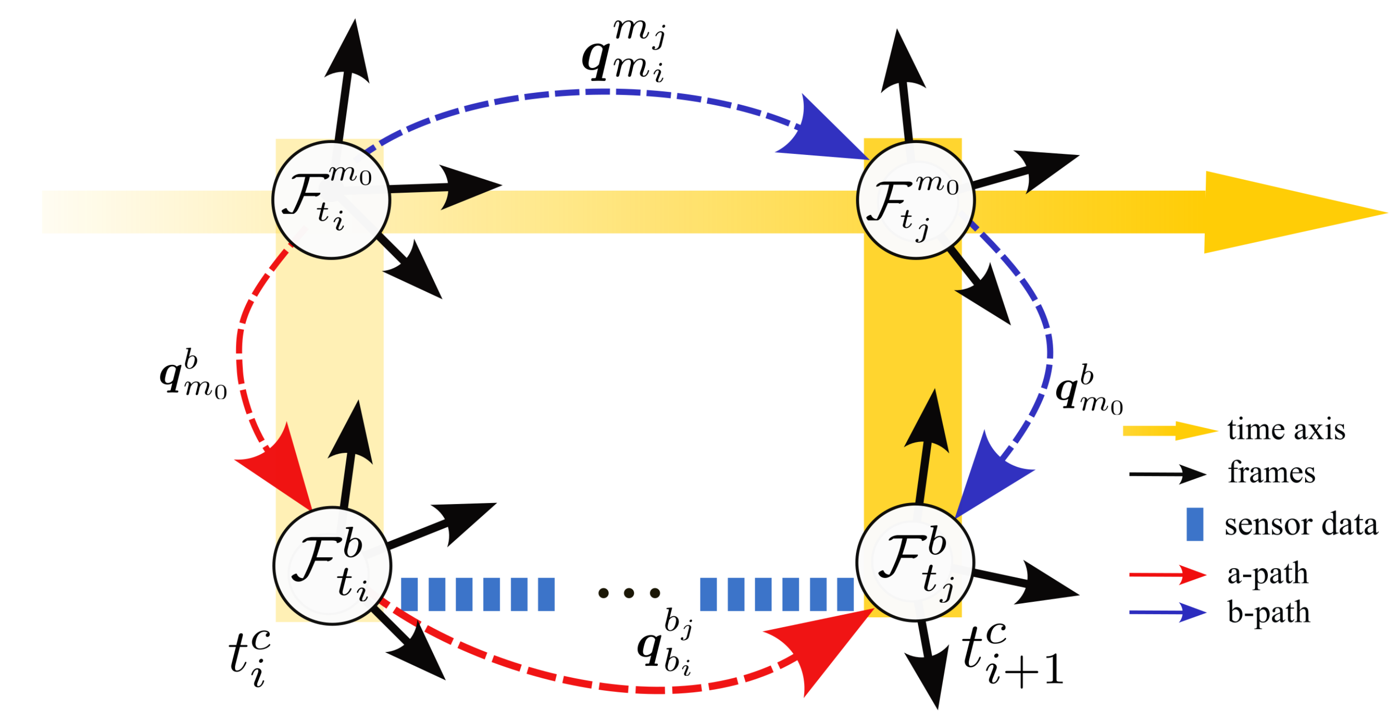
The objective of hand–eye calibration is to determine the rotational relationship between the Base Cube frame ${\mathcal{F}}^{m_0}$ and the sensor body frame ${\mathcal{F}}^b$. Figure 10 shows the method of calibration. $t_i$ and $t_j$ represent the timestamps of two adjacent images. Using the proposed visual measurement method, we measure ${\mathit{q}}_{m_0,t_i}^c$,${\mathit{q}}_{m_0,t_j}^c$ at two distinct times. Using the proposed orientation estimator, we obtain ${\mathit{q}}_{b,t_i}^I$ and ${\mathit{q}}_{b,t_j}^I$.

Based on two distinct orientation solving strategies, the following relationship can be determined:

$${\mathit{q}}_{m_0}^b\otimes {\left({\mathit{q}}_{m_0,tj}^c\right)}^{-1}\otimes {\mathit{q}}_{m_0,ti}^c={\left({\mathit{q}}_{b,tj}^I\right)}^{-1}\otimes {\mathit{q}}_{b,ti}^I\otimes {\mathit{q}}_{m_0}^b$$

(34)

Let,

$${\mathit{q}}_{m0,ti}^{m0,tj}={\left({\mathit{q}}_{m_0,tj}^c\right)}^{-1}\otimes {\mathit{q}}_{m_0,ti}^c,{\mathit{q}}_{b,ti}^{b,tj}={\left({\mathit{q}}_{b,tj}^I\right)}^{-1}\otimes {\mathit{q}}_{b,ti}^I$$

(35)

By substituting Equation (35) for Equation (34), we obtain:

$$(\mathcal{R}\left[{\mathit{q}}_{m0,ti}^{m0,tj}\right]-\mathcal{L}\left[{\mathit{q}}_{b,ti}^{b,tj}\right]){\mathit{q}}_{m_0}^b={\mathit{H}}_{t_i}^{t_j}{\mathit{q}}_{m_0}^b={\mathbf{0}}_{4\times 1}$$

(36)

By combining the aforementioned relationships across $tau$ time intervals, we are able to derive:

$${[{\left({\mathit{H}}_{t_i}^{t_j}\right)}^T,{\left({\mathit{H}}_{t_{i+1}}^{t_{j+1}}\right)}^T,\cdots ,{\left({\mathit{H}}_{t_{i+\tau -1}}^{t_{j+\tau -1}}\right)}^T]}_{4\tau \times 4}^T{\mathit{q}}_{m_0}^b=\mathcal{H}{\mathit{q}}_{m_0}^b={\mathbf{0}}_{4\tau \times 1}$$

(37)

We use the SVD decomposition method to solve Equation (37), ${\mathit{q}}_{m{1}_0}^b$ is the eigenvector corresponding to the minimum eigenvalue of ${\mathcal{H}}^T\mathcal{H}$ [37].

6. Experiment and Discussion

The testing endeavor consists of three distinct phases. Evaluation of the calibration precision of the Base Cube is the first step. We evaluate the accuracy of the adjacent marker and hand–eye calibration of the Base Cube and the influence of various PnP algorithms. In the second portion of the experiment, the accuracy of the proposed algorithm for estimating reference trajectories will be evaluated. In the first two investigations, we measure the accuracy of orientation estimation using re-projection error. The primary objective of the third experiment is to evaluate the positional precision of the proposed algorithm in relation to the measured reference trajectory. We compare and evaluate the accuracy of Madgwick, Mahony, ESKF, and proposed algorithm in relation to the reference measurement orientation. In this portion of the experiment, in order to quantitatively analyze the horizontal orientation accuracy and heading orientation accuracy of all the above estimators, quaternions are converted into Euler angles in ZYX order:

$$\left\{\begin{array}{cc}\hfill \psi & =arctan\frac{2(q_w{q}_z+q_x{q}_y)}{1-2(q_y^2+q_z^2)}\hfill \\ \hfill \theta & =arcsin2(q_w{q}_y-q_z{q}_x)\hfill \\ \hfill \varphi & =arctan\frac{2(q_w{q}_x+q_y{q}_z)}{1-2(q_x^2+q_y^2)}\hfill \end{array}\right.$$

(38)

where $\psi$, $\theta$, and $\varphi$ are the yaw angle, pitch angle, and roll angle, respectively.

6.1. Environment of Experiments

As shown in Figure 11, the experiment utilized MPU9250 [38] as an inertial–magnetic sensor, which included a tri-axis accelerometer, a tri–axis gyroscope, and a tri-axis magnetometer. The computer for running the algorithm is an ARM-based Raspberry4B [39] with $4\times$ Cortex-A57 1.5 GHz@8 GB. The MPU9250 sensor communicates with the ARM computer via the Inter-Integrated Circuit (I2C) bus, and the sensor is sampled at 150 Hz during the experiment. Before the investigation, MPU9250 is calibrated [38] and installed in an ArUco-labeled (83 × 83 (mm)) Base Cube on each surface. The tag ID of the marker begins at 0∼5 and increases in sequence. The camera used for the orientation measurement is the left-eye infrared camera of a Realsense-D435i [40], with a resolution of 848 × 480@30 Hz. Before testing, we calibrated the camera’s internal parameters and distortion coefficients with the Kalibr [36] tool.

6.2. Experiment of Calibration for Base Cube

As shown in Figure 12a–e, for the adjacent marker calibration experiment, we keep the Base Cube stationary and move the measurement camera to acquire five sets of videos containing adjacent markers (V02∼V21). During each group’s video capture, we attempt to move the camera as much as possible while ensuring that the two markers to be calibrated are within the camera’s field of view.

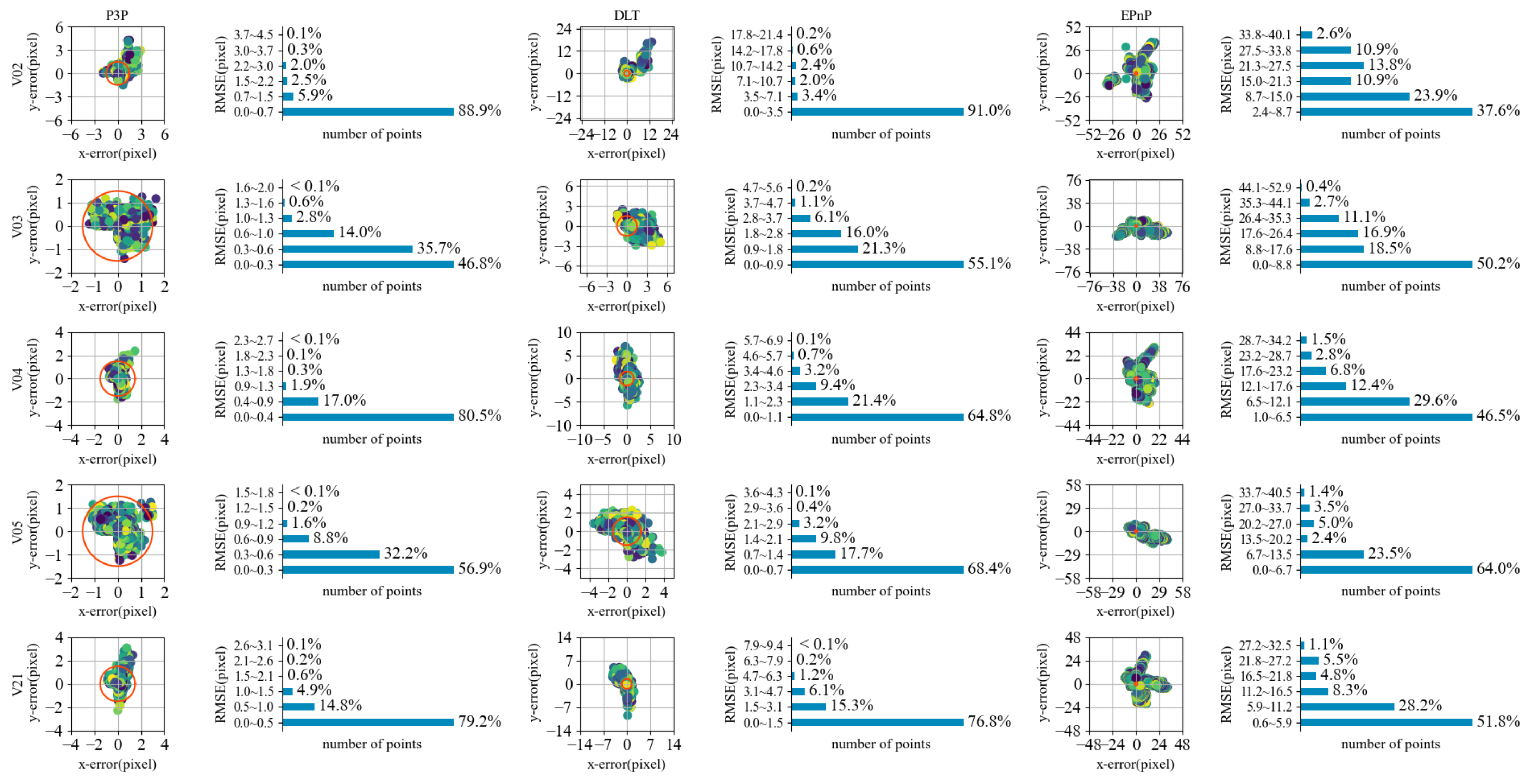
As shown in Figure 13, we first examine the distribution of re–projection error pixels using the P3P, DLT, and EPnP methods on five test sets. The test results show that the P3P method and DLT algorithm are more accurate for the test data. The variance of the error pixel distribution is marginally more remarkable in the DLT algorithm than in P3P, and P3P performs the best. The proportion of corner numbers with re–projection errors within 1 pixel is 88.9%, 96.5%, 97.5%, 97.9%, and 94.0% using the P3P algorithm. We analyze that the suboptimal performance of the EPnP algorithm may be because only four control points can be provided for each ArUco marker and that the insufficient number of control points renders the EPnP optimization iteration inadequate.

The P3P and DLT algorithms are then used to generate observation data for calibrating adjacent markers. As shown in

Table 2. The results of adjacent markers calibration.

Test Sets	Algorithm	${\mathbf{\Theta }}_{\mathit{i}\mathit{n}\mathit{i}\mathit{t}\mathit{i}\mathit{a}\mathit{l}}^{\mathit{i},\mathit{j}}$(${\mathit{rad}}^2$)	${\mathbf{\Theta }}_{\mathit{f}\mathit{i}\mathit{n}\mathit{a}\mathit{l}}^{\mathit{i},\mathit{j}}$(${\mathit{rad}}^2$)	${\mathcal{S}}_{\mathit{q}}$
V02	P3P + LM	0.14	0.12	$\left[\begin{array}{ccc}0.026671& 0.999550& 0.013753\\ 0.003705& 0.013857& -0.999897\\ -0.999637& 0.026617& 0.004074\end{array}\right]$
	P3P + DL	0.14	0.05
	DLT + LM	0.52	0.09
	DLT + DL	0.52	0.08
V03	P3P + LM	0.27	0.13	$\left[\begin{array}{ccc}-0.999812& 0.018883& 0.004257\\ 0.004184& 0.003887& 0.999984\\ 0.018899& 0.999814& 0.003808\end{array}\right]$
	P3P + DL	0.27	0.06
	DLT + LM	0.51	0.15
	DLT + DL	0.51	0.08
V04	P3P + LM	0.53	0.32	$\left[\begin{array}{ccc}0.018059& 0.002907& 0.999830\\ -0.999826& 0.004741& 0.018045\\ 0.004688& -0.999985& 0.002992\end{array}\right]$
	P3P + DL	0.53	0.06
	DLT + LM	1.22	0.21
	DLT + DL	1.22	0.08
V05	P3P + LM	0.54	0.09	$\left[\begin{array}{ccc}-0.020668& 0.015480& -0.999667\\ -0.998713& 0.046645& 0.019926\\ -0.046321& 0.998792& 0.016424\end{array}\right]$
	P3P + DL	0.54	0.08
	DLT + LM	1.14	0.15
	DLT + DL	1.14	0.24
V21	P3P + LM	0.38	0.09	$\left[\begin{array}{ccc}0.008058& 0.027544& 0.999588\\ 0.021205& -0.999391& 0.027710\\ 0.999743& 0.021420& 0.007469\end{array}\right]$
	P3P + DL	0.38	0.06
	DLT + LM	1.23	0.31
	DLT + DL	1.23	0.09

DL—Dogleg algorithm.

, we select the orientation results from 100 images with the minimum re-projection error in each test set as observation pairs for optimization and statistical analysis of the test results. ${\mathrm{\Theta }}_{initial}^{i,j}$ is the sum of squared residuals of the observed data pair (calculated using Equation (30)), while ${\mathrm{\Theta }}_{final}^{i,j}$ is the sum of squared residuals following optimization. The final column of the table displays the optimal values for calibrating the relative orientations of the five markers in set ${\mathcal{S}}_q$.

According to Table 2, the sum of the observed data pairs generated by the P3P method and the DLT method is relatively low, with a maximal value of 1.23 (approximately 0.9 deg) in the V21 dataset using the DLT algorithm. This indicates that the ArUco marker recognizes corners with high precision. Comparing the residuals before and after optimization reveals that the Dogleg and LM algorithms both obtained optimal optimization results on the dataset presented in this paper, while the P3P+DL algorithm performs the best. According to the calibration results, the relationship between the rotation matrices of several adjacent markers is qualitatively consistent with the defined coordinate system.

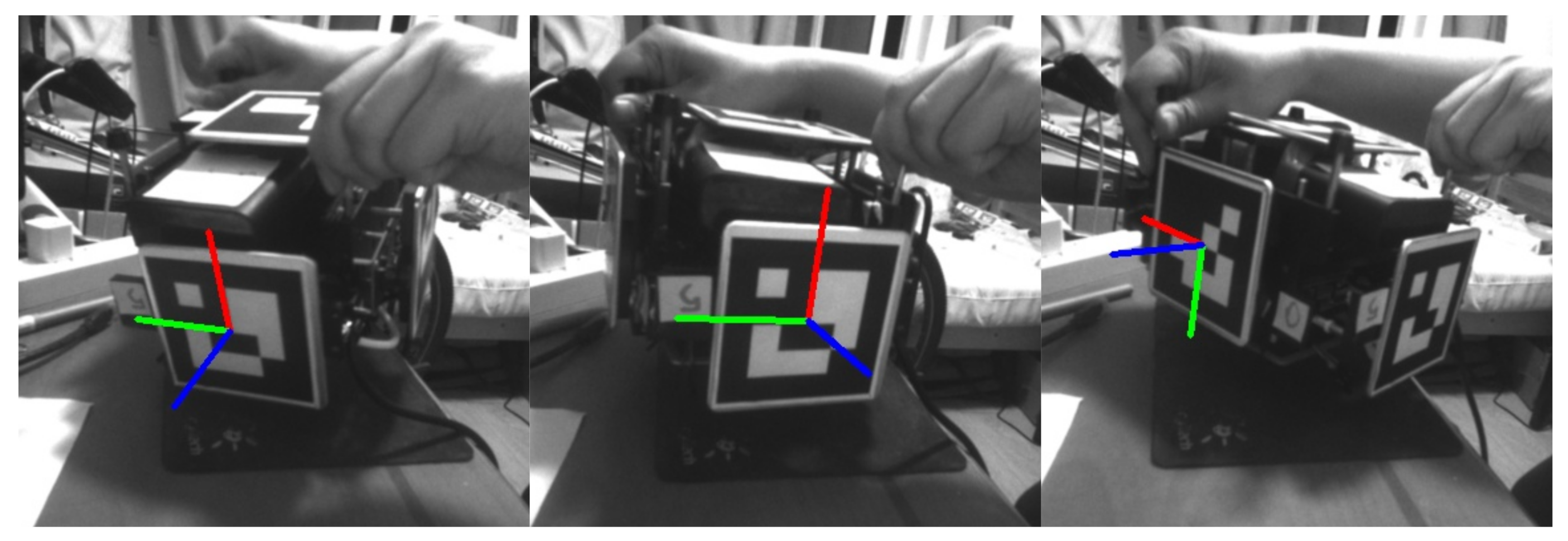
As depicted in Figure 14, we fix the camera position and rotate the Base Cube within the camera’s field of view during the hand–eye calibration experiment. Based on the calibrated result ${\mathit{q}}_{m_0}^b$, we test the error between the measurement and fusion orientations, as depicted in Figure 15. The maximal angle errors for roll, pitch, and yaw are 0.044 rad, 0.031 rad, and 0.029 rad, respectively, as depicted in the figure, which indicates that the calibration results are highly accurate.

6.3. Experiment of Orientation Measurement Accuracy

Before evaluating the performance of the proposed visual measurement algorithm, we conduct orientation measurement accuracy experiments to confirm that the orientation obtained by the proposed visual measurement method can serve as a reference pose. The test data consists of two consecutively captured recordings representing the sensor’s low–dynamic and high–dynamic conditions. In low–dynamic experiments, we endeavor to rotate the Base Cube in 3D space at various speeds as much as possible. We add more rapid movements to the high–dynamic experiments to simulate the interference of drone maneuvering acceleration. We first calculate the orientation sequences of two test data using the P3P and Dogleg optimization algorithms and then evaluate the accuracy of the solved orientation sequence and the performance of the proposed visual measurement method by calculating the mean re-projection error of the ArUco marker corners of the orientation sequence based on the corresponding image frames of the orientation sequence. The test outcomes are depicted in Figure 16. The verification results of the re-projection errors for the reference poses of the two test sets are distributed within a 2-pixel diameter circle, with average re-projection errors of 0.06 and 0.08 pixels.

6.4. Experiment of Orientation Estimation Precision

In the orientation fusion accuracy test, we align the orientation data measured from the image data in the test dataset (low–dynamic and high–dynamic datasets) with the orientation data obtained from the orientation fusion algorithm. We evaluate the orientation fusion results of the ESKF filter, Madgwick filter, and Mahony filter, in addition to the proposed algorithm, on the two test datasets.

The orientation outcomes and orientation errors (magnitude of Euler angle error in three directions) of four algorithms tested in low–dynamic settings are shown in Figure 17. The proposed estimator and the Madgwick filter react immediately to the input data, while the ESKF filter and Mahony filter first go through a convergence process. It is clear from the test results for the orientation error (the last column of the figure) that, in low–dynamic environments, the four algorithms used in the test perform similarly. We believe this is due to the high signal–to–noise ratio of the gyroscope and the sluggish maneuvering acceleration of the carrier under low–dynamic conditions (during rotation).

As depicted in Figure 18, we subsequently analyze the error of the Euler angle in detail. Without considering the convergence process, the amplitude level of heading angle error (yaw) of the four test filters is substantially greater than that of the horizontal angle error (pitch and roll), as demonstrated in the graph (ordinate scale). Comparing the last line to the other lines in the figure reveals qualitatively that the proposed algorithm has a low error angle fluctuation range. The error value for the Euler angle in Figure 18, as shown in

Table 3. A comparison of orientation errors under low–dynamic condition (rad).

Algorithm	${\mathit{\epsilon }}_{\mathit{max}}^{\mathit{norm}}$	${\mathit{\epsilon }}_{\mathit{avg}}^{\mathit{norm}}$	${\mathit{\epsilon }}_{\mathit{max}}^{\mathit{roll}}$	${\mathit{\epsilon }}_{\mathit{avg}}^{\mathit{roll}}$	${\mathit{\epsilon }}_{\mathit{max}}^{\mathit{pitch}}$	${\mathit{\epsilon }}_{\mathit{avg}}^{\mathit{pitch}}$	${\mathit{\epsilon }}_{\mathit{max}}^{\mathit{yaw}}$	${\mathit{\epsilon }}_{\mathit{avg}}^{\mathit{yaw}}$
ESKF	3.141	0.205	0.059	0.011	0.038	0.005	0.241	0.188
Madgwick	0.470	0.130	0.094	0.013	0.067	0.001	0.266	0.081
Mahony	1.205	0.136	0.158	0.016	0.062	0.004	1.185	0.076
Proposed	0.299	0.076	0.039	0.004	0.034	0.016	0.296	0.015

${\epsilon }_{}^{norm}$ represents the modular length of composite vector ${[{\epsilon }_{}^{roll},{\epsilon }_{}^{pitch},{\epsilon }_{}^{yaw}]}^T$.

, is supported by statistics. We find that the proposed estimator has an average orientation error of 0.076 rad, which is lower than those of the other three algorithms. The average value of the orientation error is 62.9% less than that of ESKF, 41.5% less than that of Madgwick, and 44.5% less than that of Mahony. The maximum value of the angular error magnitude is reduced by 75.2%, 36.3%, and 90.4%, respectively. A comparison of each Euler angle error in detail reveals that our estimates for all other indicators are optimal, except the minimum angle error amplitude of the Madgwick filter and the minimum pitch average angle error of the ESKF.

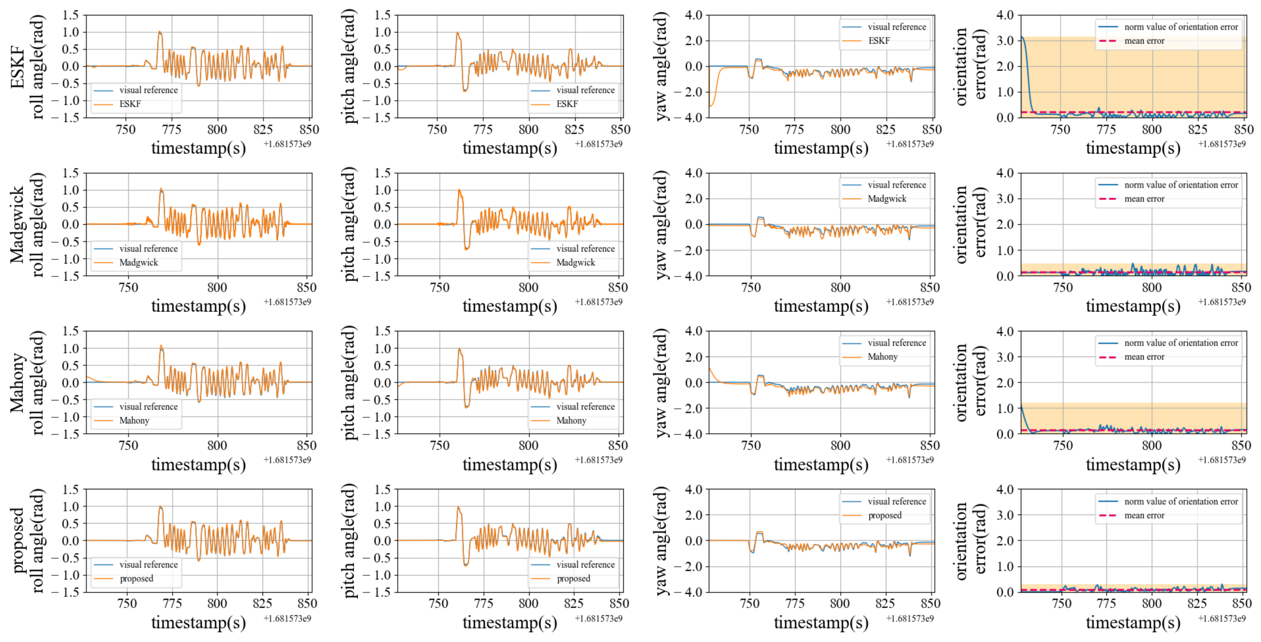
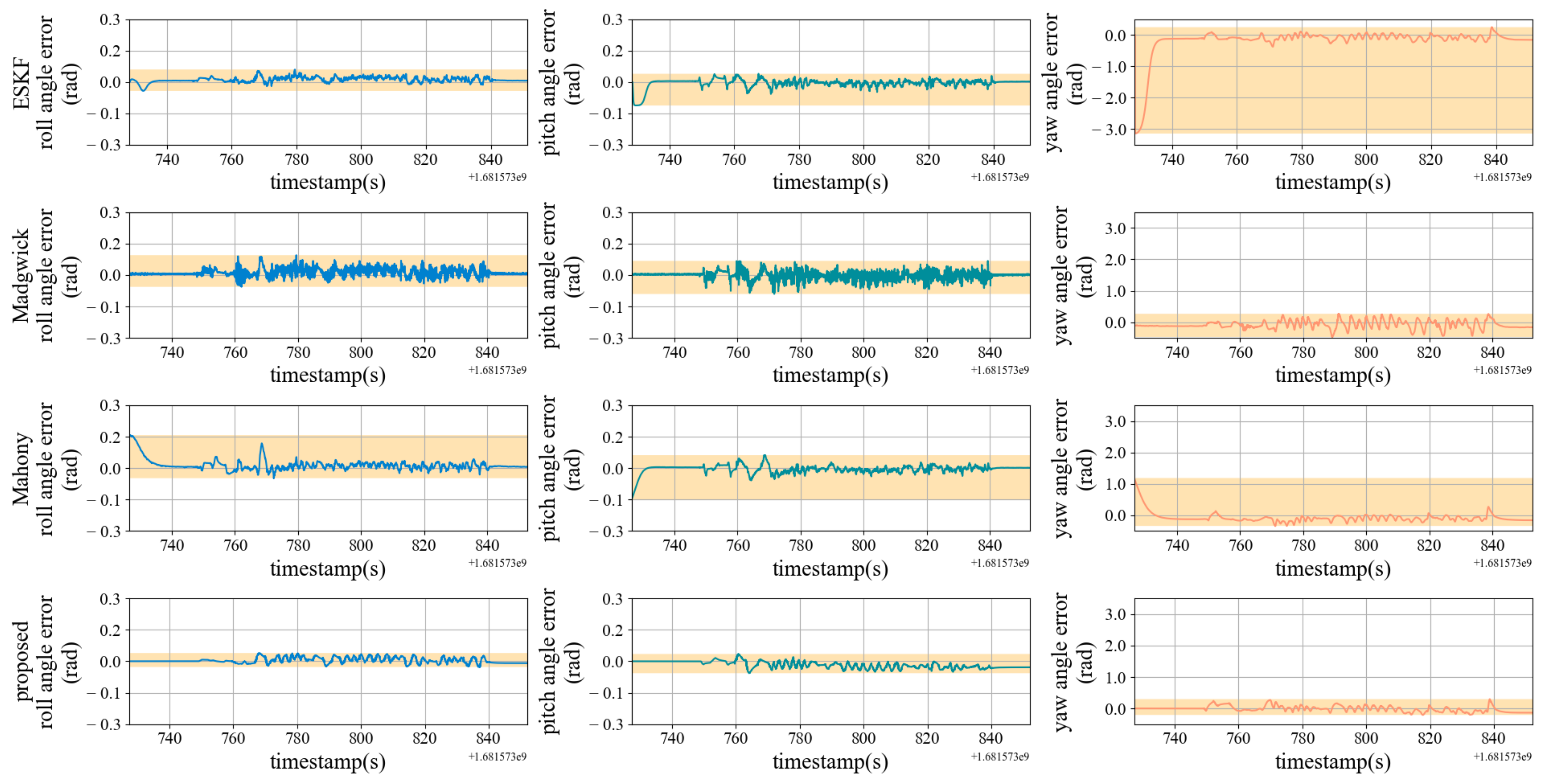
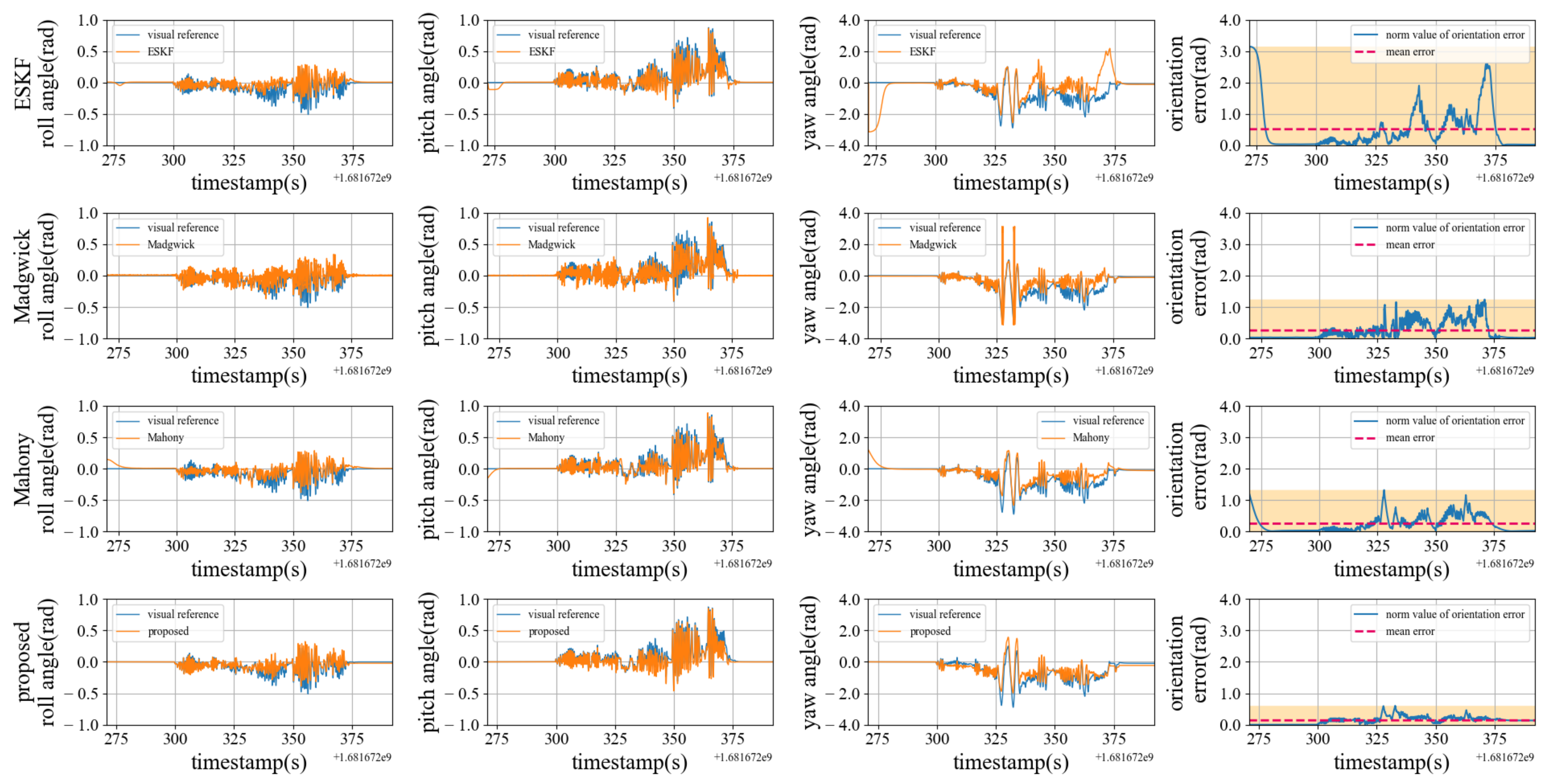
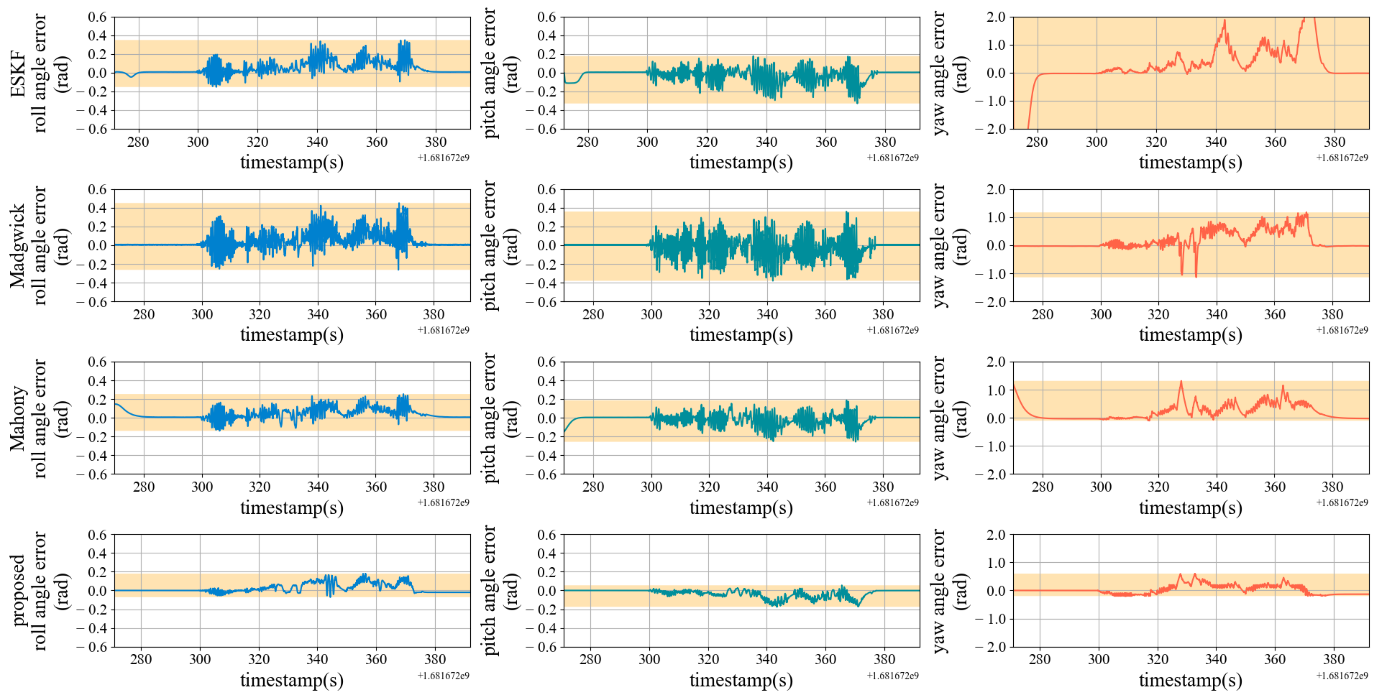
Figure 19 depicts the outcomes of a test conducted under highly dynamic conditions. The amplitude range of the angle error (the yellow area in the last column) reveals that our estimator has the smallest error fluctuation and maximum orientation accuracy. This demonstrates that the proposed estimator is able to effectively suppress the perturbation of maneuvering acceleration. Figure 20 demonstrates that among the three Euler angles, our estimator’s horizontal angle error and heading angle error are substantially better than those of other algorithms. From

Table 4. A statistical analysis of orientation errors under high–dynamic conditions (rad).

Algorithm	${\mathit{\epsilon }}_{\mathit{max}}^{\mathit{norm}}$	${\mathit{\epsilon }}_{\mathit{avg}}^{\mathit{norm}}$	${\mathit{\epsilon }}_{\mathit{max}}^{\mathit{roll}}$	${\mathit{\epsilon }}_{\mathit{avg}}^{\mathit{roll}}$	${\mathit{\epsilon }}_{\mathit{max}}^{\mathit{pitch}}$	${\mathit{\epsilon }}_{\mathit{a}\mathit{v}\mathit{g}}^{\mathit{p}\mathit{i}\mathit{t}\mathit{c}\mathit{h}}$	${\mathit{\epsilon }}_{\mathit{max}}^{\mathit{yaw}}$	${\mathit{\epsilon }}_{\mathit{avg}}^{\mathit{yaw}}$
ESKF	3.141	0.514	0.347	0.046	0.177	0.027	2.598	0.198
Madgwick	5.995	0.299	0.450	0.044	0.359	0.014	1.169	0.168
Mahony	1.324	0.253	0.254	0.044	0.187	0.016	1.317	0.217
proposed	0.600	0.138	0.179	0.021	0.055	0.030	0.598	0.029

${\epsilon }_{}^{norm}$ represents the modular length of composite vector ${[{\epsilon }_{}^{roll},{\epsilon }_{}^{pitch},{\epsilon }_{}^{yaw}]}^T$.

(statistical data of Figure 19), it can be seen that the maximum orientation errors of the proposed algorithm are 80.9%, 90.0%, and 54.6% lower than those of the ESKF, Madgwick filter, and Mahony filter, respectively. The average orientation error was 51.4%, 29.9%, and 25.5% lower, respectively. Our filter outperforms all others except the Madgwick filter, which has the most precise pitch average angle error accuracy. Combining testing under high–dynamicand low–dynamic conditions reveals that our estimator exhibits optimal performance and robustness, particularly under high–dynamic conditions.

6.5. Efficiency Test of Orientation Estimation Algorithm

In the concluding phase of the experiment, the efficiency of the proposed algorithm and three other algorithms are measured. Comparatively, we also evaluate the algorithm’s performance on the X86–64 platform. The X86–64 platform hardware environment is a laptop with an Intel I7–8750H 2.2GHz central processing unit (CPU). In the efficiency test, we conduct experiments to determine the time required by four algorithms in both high–dynamicity and low–dynamicity scenarios. The evaluation utilizes the same inertial–magnetic sensor data in the orientation estimation accuracy experiment.

Table 5. A comparison of estimation efficiency.

Test Data	Algorithm	${\mathit{t}}_{\mathit{avg}}^{\mathit{ARM}}$ (ms)	${\mathit{t}}_{\mathit{max}}^{\mathit{ARM}}$ (ms)	${\mathit{t}}_{\mathit{avg}}^{\mathit{X}86-64}$ (ms)	${\mathit{t}}_{\mathit{max}}^{\mathit{X}86-64}$ (ms)
Low dynamics	ESKF	0.913	24.998	0.164	0.276
	Madgwick	0.007	0.626	<0.001	0.018
	Mahony	0.081	3.938	0.105	0.102
	Proposed	9.781	53.269	0.102	0.109
High dynamics	ESKF	0.864	13.737	0.167	0.393
	Madgwick	0.008	1.231	<0.001	0.008
	Mahony	0.078	3.842	0.011	0.041
	Proposed	22.468	78.200	2.678	9.815

displays the time required by each algorithm to solve sensor data for a single frame.

The result in Table 5 shows that the Madgwick filter has the highest efficiency in both testing groups, and the efficiency of the proposed estimator is not significantly different from the other three algorithms. Our estimator takes longer to solve single–frame sensor data, especially in highly dynamic settings. We believe that the reason may be due to the fact that the proposed algorithm solves each input data frame iteratively, which makes the initial value of the iteration suboptimal under high–dynamic conditions, making it challenging to find the optimal orientation. On the proposed algorithm ARM platform, the average time to solve low–dynamic and high–dynamic directions is 9.78 ms (102.25 Hz) and 22.46 ms (44.52 Hz), respectively. The estimator’s output frequency can still satisfy the real–time demands of airborne navigation applications and a multi–sensor data fusion positioning apparatus. In airborne multi–sensor fusion mapping applications, for instance, the proposed estimator has a higher calculation frequency than the real–time image frame frequency (typically 30 Hz, with the human eye recognizing coherent images at a rate of 24 frames per second), allowing for more accurate direction prediction for the airborne mapping module.

7. Conclusions

Using a trust region nonlinear optimization framework, we proposed a robust orientation estimation algorithm to counteract the effect of drone maneuver acceleration on the attitude solution process and enhance direction estimation precision. We also proposed a visual attitude measurement method for evaluating the efficacy of the proposed orientation estimator. Based on measured reference orientations, we evaluated and contrasted the performance of the complementary filter, Kalman filter, and the proposed estimator under low–dynamic conditions (rotation) and high–dynamic conditions (shake). The proposed method of measuring orientation with P3P and a nonlinear optimization solver resulted in an average re–projection error of fewer than 0.1 pixels. The proposed estimator has the slightest mean orientation error under low– and high–dynamic conditions. The proposed estimator exhibits better robustness and precision under high–dynamic conditions.

References

1. Alteriis, G.; Conte, C.; Moriello, R.S.L.; Accardo, D. Use of consumer-grade MEMS inertial sensors for accurate attitude determination of drones. In Proceedings of the 2020 IEEE 7th International Workshop on Metrology for AeroSpace, Pisa, Italy, 22–24 June 2020. [Google Scholar]
2. Kuevor, P.E.; Ghaffari, M.; Atkins, E.M.; Cutler, J.W. Fast and Noise-Resilient Magnetic Field Mapping on a Low-Cost UAV Using Gaussian Process Regression. Sensors 2023, 23, 3897. [Google Scholar] [CrossRef]
3. Karam, S.; Nex, F.; Chidura, B.T.; Kerle, N. Microdrone-Based Indoor Mapping with Graph SLAM. Drones 2022, 6, 352. [Google Scholar] [CrossRef]
4. George, A.; Koivumäki, N.; Hakala, T.; Suomalainen, J.; Honkavaara, E. Visual-Inertial Odometry Using High Flying Altitude Drone Datasets. Drones 2023, 7, 36. [Google Scholar] [CrossRef]
5. He, Z.; Gao, W.; He, X.; Wang, M.; Liu, Y.; Song, Y.; An, Z. Fuzzy intelligent control method for improving flight attitude stability of plant protection quadrotor UAV. Int. J. Agric. Biol. Eng. 2019, 12, 110–115. [Google Scholar]
6. Flores, D.A.; Saito, C.; Paredes, J.A.; Trujillano, F. Aerial photography for 3D reconstruction in the Peruvian Highlands through a fixed-wing UAV system. In Proceedings of the IEEE International Conference on Mechatronics (ICM), Akamatsu, Japan, 6–9 August 2017.
7. Nazarahari, M.; Rouhani, H. Sensor fusion algorithms for orientation tracking via magnetic and inertial measurement units: An experimental comparison survey. Inf. Fusion 2021, 76, 8–23. [Google Scholar] [CrossRef]
8. Li, X.; Xu, Q.; Shi, Q.; Tang, Y. Complementary Filter for orientation Estimation Based on MARG and Optical Flow Sensors. J. Phy. Conf. Ser. 2021, 2010, 012160. [Google Scholar] [CrossRef]
9. Park, S.; Park, J.; Park, C.G. Adaptive orientation estimation for low-cost MEMS IMU using ellipsoidal method. IEEE Trans. Instrum. Meas. TTM 2020, 9, 7082–7091. [Google Scholar] [CrossRef]
10. Mahony, R.; Hamel, T.; Pflimlin, J.M. Nonlinear complementary filters on the special orthogonal group. IEEE Trans. Autom. Control TAC 2008, 5, 1203–1218. [Google Scholar] [CrossRef]
11. Madgwick, S.O.; Harrison, A.J.; Vaidyanathan, R. Estimation of IMU and MARG orientation using a gradient descent algorithm. In Proceedings of the IEEE International Conference on Rehabilitation Robotics, Zurich, Switzerland, 29 June–1 July 2011. [Google Scholar]
12. Sabatini, A.M. Quaternion-based extended Kalman filter for determining orientation by inertial and magnetic sensing. IEEE Trans. Biomed. Eng. 2006, 53, 1346–1356. [Google Scholar] [CrossRef]
13. Vitali, R.V. McGinnis, R.S. and Perkins, N.C., Robust error-state Kalman filter for estimating IMU orientation. IEEE Sens. J. 2020, 3, 3561–3569. [Google Scholar]
14. Sola, J. Quaternion kinematics for the error-state Kalman filter. arXiv 2017, arXiv:1711.02508. [Google Scholar]
15. Soliman, A.; Ribeiro, G.A.; Torres, A.; Rastgaar, M. Error-state Kalman filter for online evaluation of ankle angle. In Proceedings of the International Conference on Advanced Intelligent Mechatronics (AIM), Sapporo, Japan, 11–15 July 2022. [Google Scholar]
16. Kam, H.C.; Yu, Y.K.; Wong, K.H. An improvement on aruco marker for pose tracking using kalman filter. In Proceedings of the 19th IEEE/ACIS International Conference on Software Engineering, Artificial Intelligence, Networking and Parallel/Distributed Computing, Busan, Republic of Korea, 27–29 June 2018. [Google Scholar]
17. Marut, A.; Wojtowicz, K.; Falkowski, K. ArUco markers pose estimation in UAV landing aid system. In Proceedings of the IEEE 5th International Workshop on Metrology for AeroSpace, Trento, Italy, 19–21 June 2019. [Google Scholar]
18. Lu, X.X. A Review of Solutions for Perspective-n-Point Problem in Camera Pose Estimation. J. Phys. Conf. Ser. 2018, 5, 052009. [Google Scholar] [CrossRef]
19. Qin, T.; Li, P.; Shen, S. Vins-mono: A robust and versatile monocular visual-inertial state estimator. IEEE Trans. Robot. 2018, 34, 1004–1020. [Google Scholar] [CrossRef]
20. Westman, E.; Hinduja, A.; Kaess, M. Feature-based SLAM for imaging sonar with under-constrained landmarks. In Proceedings of the IEEE International Conference on Robotics and Automation (ICRA), Brisbane, Australia, 21–25 May 2018. [Google Scholar]
21. Yuan, Y.X. Recent advances in trust region algorithms. Math. Program. 2015, 151, 249–281. [Google Scholar] [CrossRef]
22. Jafari, H.; Shahmiri, F. Examination of Quadrotor Inverse Simulation Problem Using Trust-Region Dogleg Solution Method. J. Aerosp. Sci. Technol. 2019, 12, 39–51. [Google Scholar]
23. iplimage, P3P. Available online: http://iplimage.com/blog/p3p-perspective-point-overview/ (accessed on 5 April 2023).
24. Gao, X.S.; Hou, X.R.; Tang, J.; Cheng, H.F. Complete solution classification for the perspective-three-point problem. IEEE Trans. Pattern Anal. Mach. Intell. 2003, 25, 930–943. [Google Scholar]
25. Li, S.; Xu, C. A stable direct solution of perspective-three-point problem. Int. J. Pattern Recognit. Artif. Intell. 2011, 25, 627–642. [Google Scholar] [CrossRef]
26. Hesch, J.A.; Roumeliotis, S.I. A Direct Least-Squares (DLS) method for PnP. In Proceedings of the IEEE International Conference on Computer Vision (ICCV), Barcelona, Spain, 6–13 November 2011. [Google Scholar]
27. Lepetit, V.; Moreno-Noguer, F.; Fua, P. EPnP: Efficient Perspective-n-Point Camera Pose Estimation. Int. J. Comput. Vis. 2009, 81, 155–166. [Google Scholar] [CrossRef]
28. Penate-Sanchez, A.; Andrade-Cetto, J.; Moreno-Noguer, F. Exhaustive linearization for robust camera pose and focal length estimation. IEEE Trans. Pattern Anal. Mach. Intell. TPAMI 2013, 10, 2387–2400. [Google Scholar] [CrossRef]
29. Garrido-Jurado, S.; Muñoz-Salinas, R.; Madrid-Cuevas, F.J.; Medina-Carnicer, R. Generation of fiducial marker dictionaries using mixed integer linear programming. Pattern Recognit. 2016, 51, 481–491. [Google Scholar] [CrossRef]
30. Romero-Ramirez, F.J.; Muñoz-Salinas, R.; Medina-Carnicer, R. Speeded up detection of squared fiducial markers. Image Vis. Comput. 2018, 76, 38–47. [Google Scholar] [CrossRef]
31. Filus, K.; Sobczak, Ł; Domańska, J.; Domański, A.; Cupek, R. Real-time testing of vision-based systems for AGVs with ArUco markers. In Proceedings of the IEEE International Conference on Big Data, Osaka, Japan, 17–20 December 2022. [Google Scholar]
32. Kalaitzakis, M.; Carroll, S.; Ambrosi, A.; Whitehead, C.; Vitzilaios, N. Experimental Comparison of Fiducial Markers for Pose Estimation. In Proceedings of the International Conference on Unmanned Aircraft Systems (ICUAS), Nagoya, Japan, 23–25 March 2020. [Google Scholar]
33. MacTavish, K.; Barfoot, T.D. At all Costs: A Comparison of Robust Cost Functions for Camera Correspondence Outliers. In Proceedings of the Conference on Computer and Robot Vision, Halifax, UK, 3–5 June 2015. [Google Scholar]
34. Kümmerle, R.; Grisetti, G.; Strasdat, H.; Konolige, K.; Burgard, W. g2o: A general framework for graph optimization. In Proceedings of the IEEE International Conference on Robotics and Automation, Shanghai, China, 9–13 May 2011. [Google Scholar]
35. Ceres Solver. Available online: https://github.com/ceres-solver/ceres-solver (accessed on 2 April 2023).
36. Furgale, P.; Rehder, J.; Siegwart, R. Unified Temporal and Spatial Calibration for Multi-Sensor Systems. In Proceedings of the 2013 IEEE/RSJ International Conference on Intelligent Robots and Systems, Tokyo, Japan, 3–8 November 2013. [Google Scholar]
37. Hartley, R.; Zisserman, A. Numerical Method. In Multiple View Geometry in Computer Vision, 2nd ed.; Cambridge University Press: Cambridge, UK, 2003; p. 412. [Google Scholar]
38. InvenSense MPU9250. Available online: https://invensense.tdk.com/products/motion-tracking/9-axis/mpu-9250/ (accessed on 2 April 2023).
39. Pi-4-model-b. Available online: https://www.raspberrypi.com/products/raspberry-pi-4-model-b/ (accessed on 2 April 2023).
40. Intel Realsense D435i. Available online: https://www.intelrealsense.com/depth-camera-d435i/ (accessed on 2 April 2023).
Figure 1. Description of Perspective–n–Point (PnP) Algorithm. The objective of the algorithm is to determine the relative rotation R r c R 3 × 3 and translation t r c R 3 between the reference frame and the camera frame. p i r R 3 represents one of the object points in the reference coordinate system. p ¯ i r R 2 represents the corresponding image point of p i r in the normalized camera frame.
Drones 07 00351 g001
Figure 2. The patterns of Augmented Reality University of Cordoba (ArUco) marker. The sequence of marker patterns’ ID from left to right is 0∼5.
Drones 07 00351 g002
Figure 3. A pipeline of the proposed algorithm consists of two components, robust orientation estimator (yellow part) and measurement of sensor orientation (blue part). Only the stereo camera’s left eye is utilized in the online measurement procedure.
Drones 07 00351 g003
Figure 4. An overview of the coordinate system used in this paper.
Drones 07 00351 g004
Figure 5. A schematic of geomagnetic vector rotation. To determine the heading angle uniquely, we rotate m ˇ I , k about the z-axis of the reference frame F I in the YOZ plane to obtain m ^ I , k .
Drones 07 00351 g005
Figure 6. A pipeline of proposed estimator.
Drones 07 00351 g006
Figure 7. A pipeline of the proposed method for orientation measurement. The proposed method involves offline calibration and online measurement steps. The segment on offline calibration consists of two steps: calibration of markers and calibration of hand–eye.
Drones 07 00351 g007
Figure 8. A pinhole model of the camera. The camera model specifies the projection relationship between object points in the reference frame and image points in the pixel frame.
Drones 07 00351 g008
Figure 9. The overview of Base Cube, which is used as a measurement standard. (a,b) depict the placement of six ArUco markers on the outer surface, while (c) depicts the calibrated path and associated variables. The calibration objective is to identify the five relative rotations in S q .
Drones 07 00351 g009
Figure 10. A schematic depiction of the hand–eye calibration method. We obtain q m 0 , t i b , t j along two distinct paths (red path and blue path) and formulate the least squares problem in order to solve q m 0 b . The yellow gradient arrow in the figure represents the timeline, and the timeline’s vertical trajectory represents the same period.
Drones 07 00351 g010
Figure 11. The hardware experiment environment. The MPU9250 (right sub-image) sensor is mounted on an orthogonal reference bracket within the Base Cube. The left sub-image shows the Raspberry4B computer.
Drones 07 00351 g011
Figure 12. Image samples of the test set used for calibration of adjacent markers. The subgraphs (ae) represent randomly selected patterns from videos of test sets V02, V03, V04, V05, and V21, respectively. The test set names correspond to the subscripts of the variables in S q .
Drones 07 00351 g012
Figure 13. The performance comparison of PnP algorithms. The PnP algorithm is used to generate data pairings to calibrate adjacent markers. This figure depicts the pixel coordinate distribution of re–projection error for each ArUco marker in five test videos utilizing the participating P3P, DLT, and EPnP algorithms. Each vertical column represents the V02, V03, V04, V05, and V21 test sets. The effects of the P3P, DLT, and EPnP algorithms are depicted from left to right. The regions within the red circle represent regions with a 1-pixel re–projection error. The points of different colors in the scatterplot section are to distinguish adjacent points.
Drones 07 00351 g013
Figure 14. The visualization of hand–eye calibration.
Drones 07 00351 g014
Figure 15. The error results of hand–eye calibration. The left, center, and right images depict the angle errors following roll, pitch, and yaw calibration, respectively.
Drones 07 00351 g015
Figure 16. The distribution of visual measurement orientation re–projection error. (a,b) represent the statistical information of the re-projection error of two image sequences (low–dynamic and high–dynamic) utilized to evaluate the orientation estimation algorithms. The scatter plot illustrates the distribution of re–projection error points within the pixel plane. The points of different colors in the scatterplot section are to distinguish adjacent points.
Drones 07 00351 g016
Figure 17. A comparison of orientation estimation results under low–dynamic conditions.
Drones 07 00351 g017
Figure 18. A comparison of orientation errors in Euler angle under low–dynamic conditions. Each row from top to bottom represents the test result of ESKF, Madgwick filter, Mahony filter, and proposed estimator. Each column from left to right displays the comparison results for roll, pitch, and yaw angle in that order.
Drones 07 00351 g018
Figure 19. A comparison of orientation estimation results in under high–dynamic conditions.
Drones 07 00351 g019
Figure 20. A comparison of orientation errors in Euler angle under high–dynamic conditions. Each row from top to bottom represents the test result of ESKF, Madgwick filter, Mahony filter, and proposed estimator. Each column from left to right displays the comparison results for roll, pitch, and yaw angle in that order.
Drones 07 00351 g020