
Towards More Efficient Electric Propulsion UAV Systems Using Boundary Layer Ingestion


Abstract
:1. Introduction
2. Materials and Methods
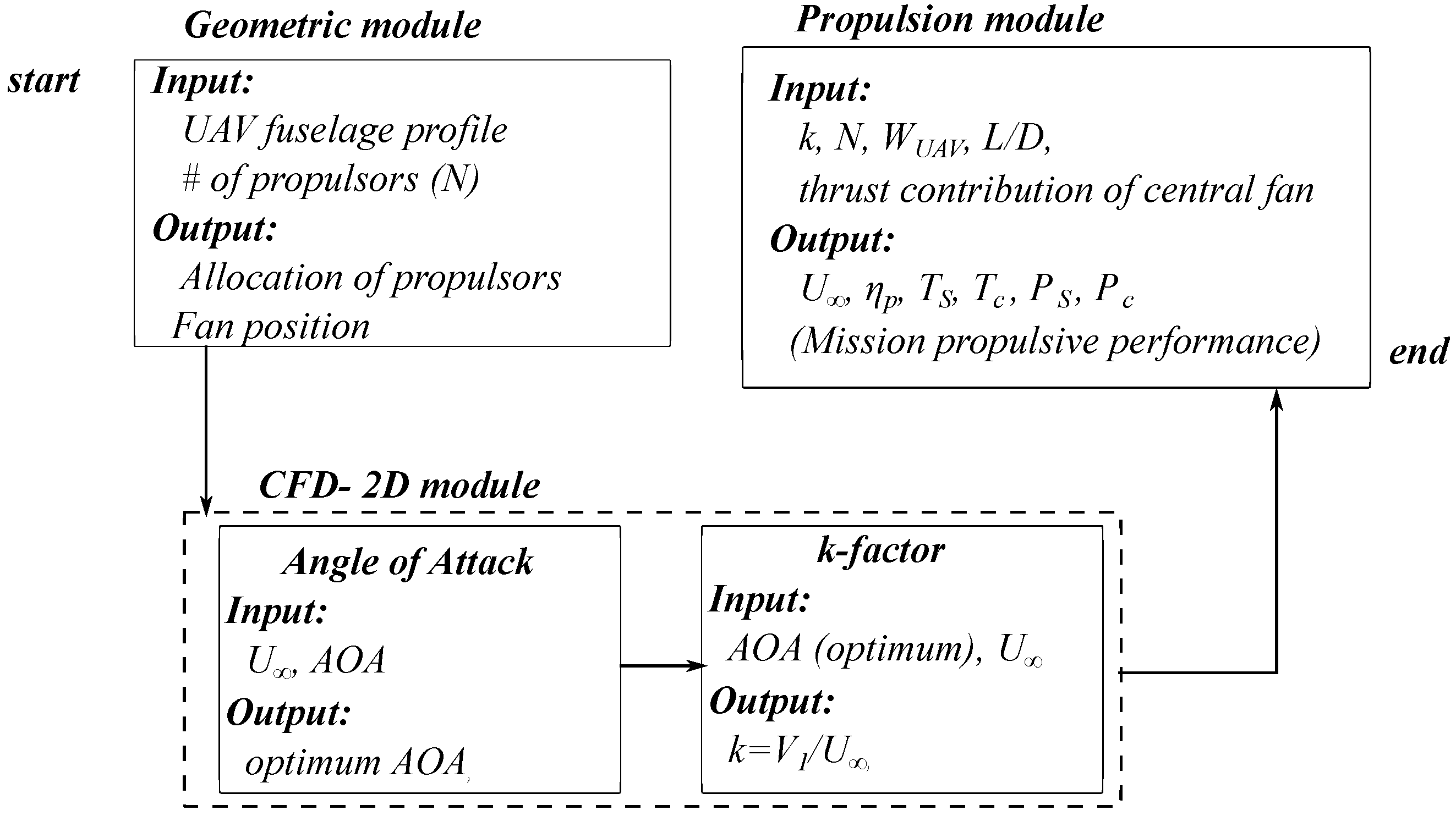
2.1. Framework of Analysis
UAV Characteristics
2.2. Geometric Module
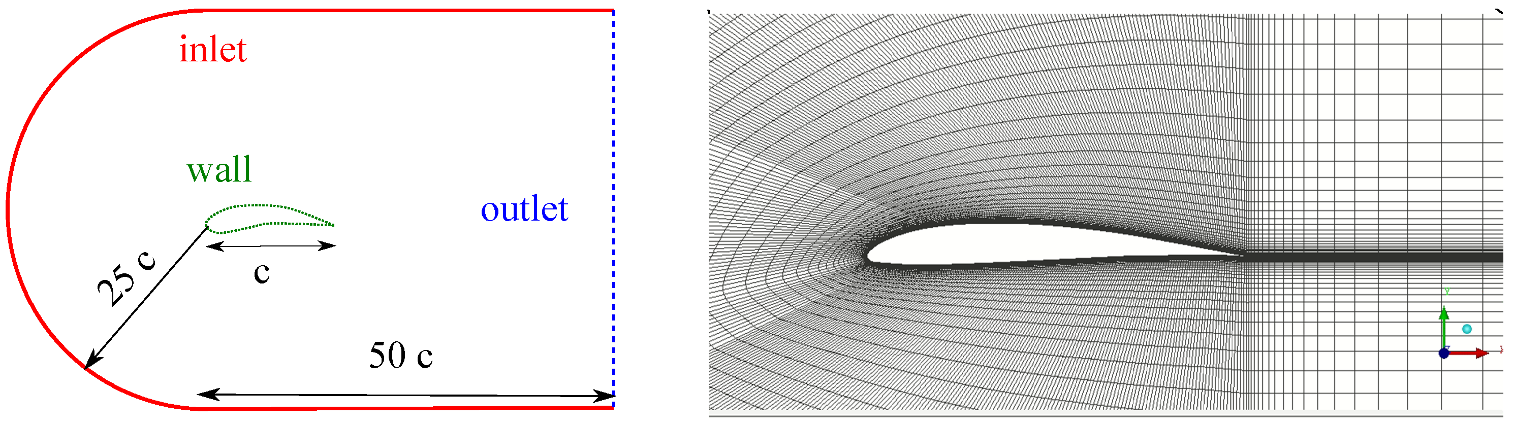
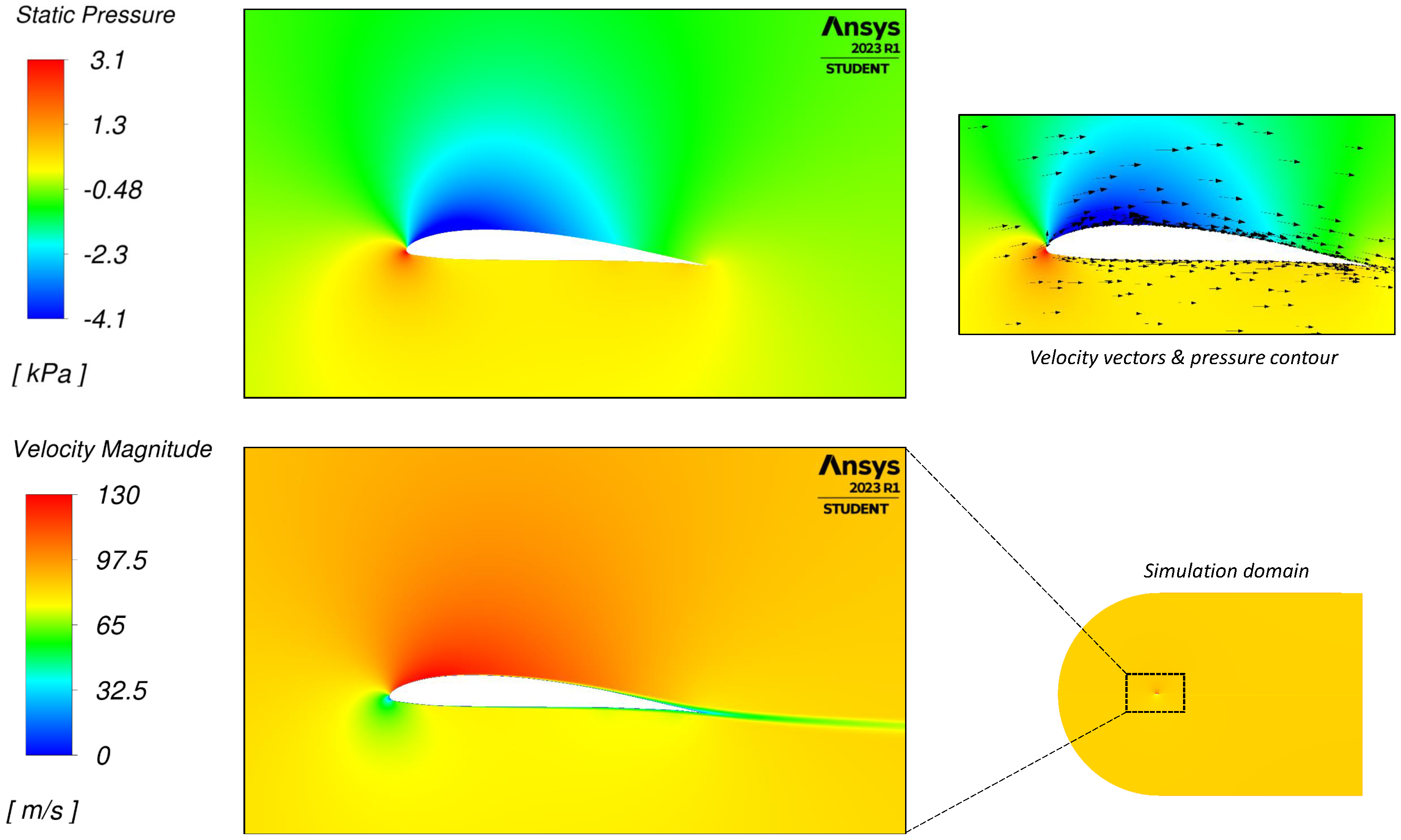
2.3. In-House CFD Case Study
Mesh and Boundary Conditions
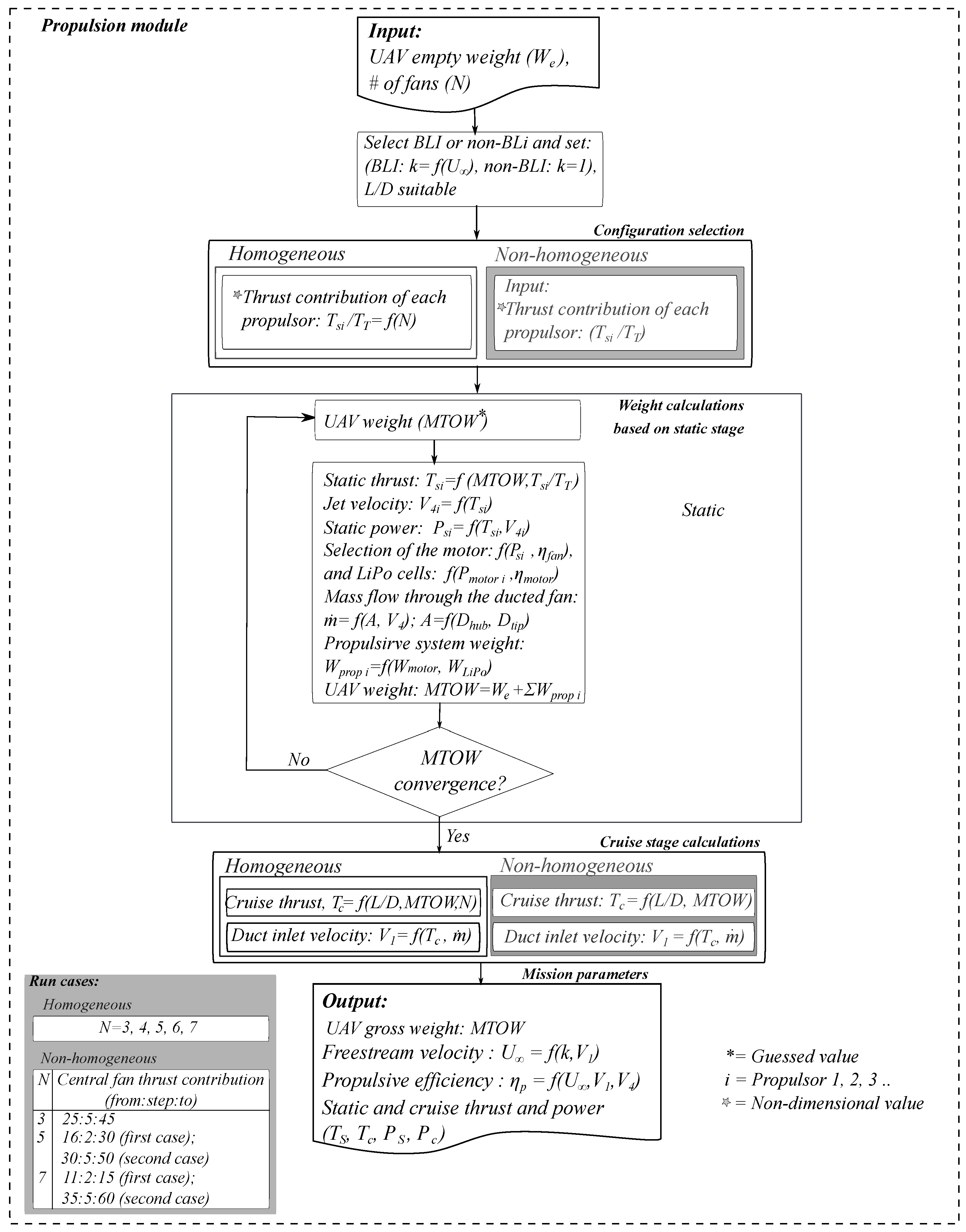
2.4. Propulsion Module
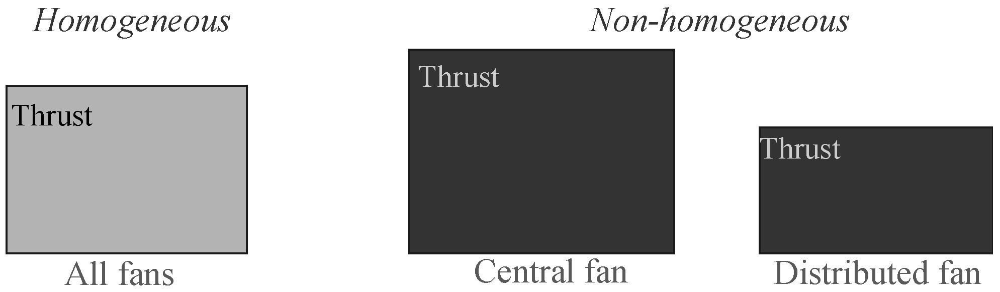
2.4.1. Parametric Formulation for Thrust Contribution
2.4.2. Static Stage Model
2.4.3. Distributed Propulsion
2.4.4. Weight Estimation
3. Results
3.1. In-House CFD Case Study
3.2. Propulsion Module
3.2.1. Homogeneous Configuration
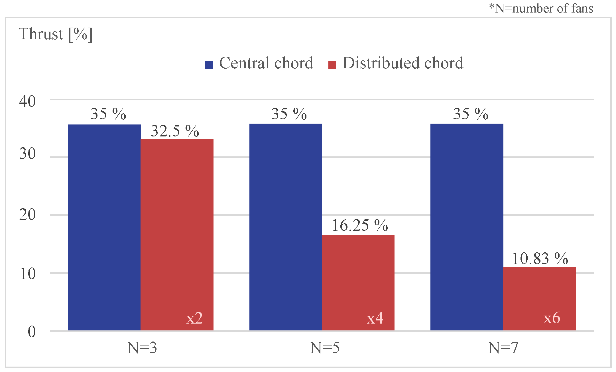
3.2.2. Non-Homogeneous Configurations
- Static Performance
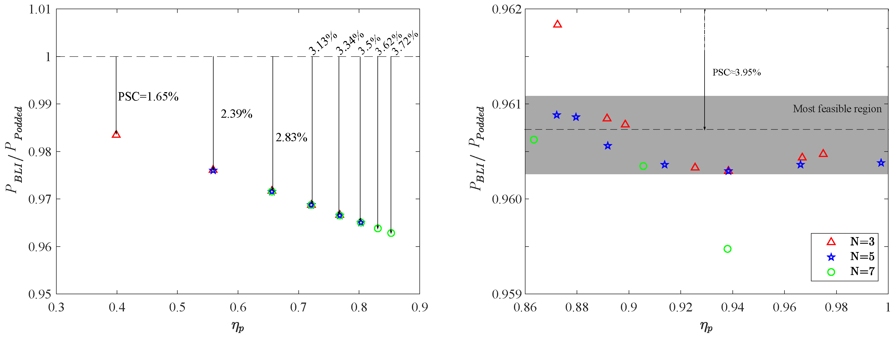
- Cruise performance
3.3. Validation
4. Discussion
5. Conclusions
Author Contributions
Funding
Data Availability Statement
Acknowledgments
Conflicts of Interest
References
- Bruner, S.; Baber, S.; Harris, C.; Caldwell, N.; Keding, P.; Rahrig, K.; Pho, L.; Wlezian, R. NASA N+ 3 Subsonic Fixed Wing Silent Efficient Low-Emissions Commercial Transport (SELECT) Vehicle Study. Revision A; NASA/CR: Cleveland, OH, USA, 2010; pp. 1–187.
- Abbas, A.; De Vicente, J.; Valero, E. Aerodynamic technologies to improve aircraft performance. Aerosp. Sci. Technol. 2013, 28, 100–132. [Google Scholar] [CrossRef]
- NASA Technical Reports Server. Review of Propulsion Technologies for N+ 3 Subsonic Vehicle Concepts; AIAA: Cleveland, OH, USA, 2011. [Google Scholar]
- Valencia, E.A.; Ayala, M.; Hidalgo, V.; Simbaña, S.; Alulema, V.H.; Rodriguez, D.; Cando, E. Aeropropulsive Evaluation of Boundary Layer Ingestion for Medium Electric-Powered UAVs. In Proceedings of the AIAA Propulsion and Energy 2020 Forum, Virtual Event, 24–28 August 2020; Volume 1, pp. 1–16. [Google Scholar]
- Plas, A.; Crichton, D.; Sargeant, M.; Hynes, T.; Greitzer, E.; Hall, C.; Madani, V. Performance of a bOundary Layer Ingesting (BLI) Propulsion System; Session: AD-3: The Silent Aircraft Initiative; AIAA: Orlando, FL, USA, 2007. [Google Scholar]
- NASA Technical Reports Server. Turboelectric Distributed Propulsion Engine Cycle Analysis for Hybrid-Wing-Body Aircraft; AIAA: Orlando, FL, USA, 2009. [Google Scholar]
- Liu, C. Turboelectric Distributed Propulsion System Modelling. Ph.D. Dissertation, Cranfield University, Bedford, UK, 2013. [Google Scholar]
- Goldberg, C.; Nalianda, D.; Pilidis, P.; MacManus, D.; Felder, J. Installed performance assessment of a boundary layer ingesting distributed propulsion system at design point. J. Propuls. Power 2016, 52, 1–22. [Google Scholar]
- Habermann, A. Effects of Distributed Propulsion on Wing Mass in Aircraft Conceptual Design; AIAA: Orlando, FL, USA, 2020; Volume 2625. [Google Scholar]
- Diamantidou, D.E.; Hosain, M.L.; Kyprianidis, K.G. Recent Advances in Boundary Layer Ingestion Technology of Evolving Powertrain Systems. Sustainability 2022, 14, 1731. [Google Scholar] [CrossRef]
- Budziszewski, N.; Friedrichs, J. Modelling of a Boundary Layer Ingesting propulsor. Energies 2018, 11, 708. [Google Scholar] [CrossRef]
- Drela, M. Power Balance in Aerodynamic Flows. AIAA J. 2012, 47, 1761–1771. [Google Scholar] [CrossRef]
- Arntz, A.; Atinault, O.; Destarac, D.; Merlen, A. Exergy-Based Aircraft Aeropropulsive Performance Assessment: CFD Application to Boundary Layer Ingestion; AIAA: Orlando, FL, USA, 2014; Volume 2573. [Google Scholar]
- Hall, D.K.; Huang, A.C.; Uranga, A.; Greitzer, E.M.; Drela, M.; Sato, S. Boundary Layer Ingestion Propulsion Benefit for Transport Aircraft. J. Propuls. Power 2017, 33, 1118–1129. [Google Scholar] [CrossRef]
- Risch, T.; Cosentino, G.; Regan, C.; Kisska, M.; Princen, N. X-48B Flight-Test Progress Overview. In Proceedings of the 47th AIAA Aerospace Sciences Meeting Including the New Horizons Forum and Aerospace Exposition, AIAA, Orlando, FL, USA, 5–8 January 2009. [Google Scholar]
- Griffin, B.; Brown, N.; Yoo, S. Intelligent Control for Drag Reduction on the X-48B Vehicle. In Proceedings of the AIAA Guidance, Navigation, and Control Conference, Portland, OR, USA, 8–11 August 2011. [Google Scholar]
- Bevilaqua, P.; Yam, C. Propulsion Efficiency of Wake Ingestion. J. Propuls. Power 2020, 36, 517–526. [Google Scholar] [CrossRef]
- Menter, F.R. Two-equation eddy-viscosity turbulence models for engineering applications. AIAAJ 1994, 32, 1598–1609. [Google Scholar] [CrossRef]
- Montgomery, L. Aerodynamic Experiments on a Ducted Fan in Hover and Edgewise Flight. Master’s Thesis, The Pennsylvania State University, State College, PA, USA, 2009. [Google Scholar]
- Jin, Y.; Qian, Y.; Zhang, Y.; Zhuge, W. Modeling of Ducted-Fan and Motor in an Electric Aircraft and a Preliminary Integrated Design. J. Aerosp. 2018, 11, 115–126. [Google Scholar] [CrossRef]
- Akturk, A.; Camci, C. Tip Clearance Investigation of a Ducted Fan Used in VTOL UAVS: Part 1—Baseline Experiments and Computational Validation. J. Turbomach. 2011, 7, 331–344. [Google Scholar]
- Brushless Motors. Available online: https://www.turbines-rc.com/en/25-brushless-motors (accessed on 14 April 2023).
- Rodriguez, D.L. Multidisciplinary optimization method for designing boundary-layer-ingesting inlets. J. Aircr. 2009, 46, 883–894. [Google Scholar] [CrossRef]
- Uranga, A.; Drela, M.; Hall, D.K.; Greitzer, E.M. Analysis of the Aerodynamic Benefit from Boundary Layer Ingestion for Transport Aircraft. AIAA J. 2008, 56, 4271–4281. [Google Scholar] [CrossRef]
- EDF & Turbines. Available online: https://www.turbines-rc.com/en/132-schubeler (accessed on 16 April 2023).
- Selig, M.S.; Guglielmo, J.J.; Broeren, A.P.; Giguere, P. Summary of Low-Speed Airfoil Data; SoarTech Publications: Virginia Beach, VA, USA, 1995; Volume 1. [Google Scholar]


| Feature | MTOW | Propulsive Eff. |
|---|---|---|
| Actual | 226 kg (including 3 jets | not given |
| and 13 gallons of fuel [15]) | ||
| Desired Design | <226 kg | >85% |
| Motor Class | Power (P) [W] | Weight (W) | LiPo Batteries |
|---|---|---|---|
| (Diameter [mm]) | Min.–Max. | [kg] | [cells] |
| 24 | 315–525 | 0.055 | 4 |
| 29 | 1075–1950 | 0.175 | 6 |
| 36 | 1950–2425 | 0.275 | 8 |
| 40 | 2975–4425 | 0.450 | 12 |
| 50 | 4425–9625 | 0.600 | 14 |
| 56 | 9625–14,000 | 1.020 | 19 |
| Number of | Motor Diameter, | Total Thrust, N | Total Power, kW | Weight, kg |
|---|---|---|---|---|
| Propulsors (N) | cm | () | () | UAV () |
| 3 | 5.6 | 581.06 | 26.28 | 197.70 |
| 4 | 5 | 573.91 | 25.02 | 195.27 |
| 5 | 5 | 573.57 | 22.36 | 195.15 |
| 6 | 5 | 575.40 | 20.51 | 195.77 |
| 7 | 5 | 578.20 | 20.37 | 198.02 |
| Number of | Total Thrust | Total Power , kW | ||||
|---|---|---|---|---|---|---|
| Propulsors (N) | BLI | Podded | BLI | Podded | BLI | Podded |
| 3 | 113.772 | 119.079 | 9.284 | 9.668 | 0.938 | 0.886 |
| 4 | 112.371 | 117.612 | 8.840 | 9.205 | 0.938 | 0.886 |
| 5 | 112.305 | 117.544 | 7.899 | 8.226 | 0.938 | 0.886 |
| 6 | 112.663 | 117.918 | 7.246 | 7.545 | 0.938 | 0.886 |
| 7 | 111.748 | 117.063 | 7.112 | 7.412 | 0.938 | 0.885 |
| Number of | Central Fan Thrust | Thrust, N | Power, kW | UAV Weight | ||||
|---|---|---|---|---|---|---|---|---|
| Propulsors (N) | Contribution, % | Total () | Central | Distrib. | Total () | Central | Distrib. | (), kg |
| 3 | 25 | 563.462 | 143.477 | 209.993 | 26.035 | 6.256 | 9.890 | 191.71 |
| 35 | 566.405 | 198.241 | 184.075 | 25.319 | 9.369 | 7.975 | 192.71 | |
| 45 | 568.697 | 261.623 | 153.537 | 27.603 | 13.753 | 6.925 | 193.50 | |
| 5 | 16 | 576.811 | 92.352 | 121.115 | 22.786 | 3.379 | 4.852 | 196.25 |
| 22 | 573.571 | 126.435 | 112.054 | 22.361 | 5.175 | 4.318 | 195.15 | |
| 30 | 576.811 | 173.021 | 98.173 | 22.030 | 7.397 | 3.541 | 195.42 | |
| 7 | 11 | 576.142 | 63.059 | 85.514 | 20.579 | 2.278 | 3.050 | 196.03 |
| 13 | 577.068 | 74.626 | 83.740 | 20.718 | 2.933 | 2.964 | 196.34 | |
| 15 | 576.954 | 86.401 | 81.759 | 23.280 | 3.098 | 3.364 | 196.30 | |
| Number of | Central Fan Thrust | Total Thrust | Total Power , kW | , - | |||
|---|---|---|---|---|---|---|---|
| Propulsors, | Contribution, % | BLI | Podded | BLI | Podded | BLI | Podded |
| 3 | 25 | 109.944 | 115.242 | 5.914 | 6.013 | 0.399 | 0.329 |
| 35 | 110.868 | 116.211 | 7.449 | 7.667 | 0.656 | 0.598 | |
| 45 | 111.376 | 116.744 | 9.217 | 9.536 | 0.768 | 0.713 | |
| 5 | 35 | 110.868 | 116.211 | 7.449 | 7.667 | 0.656 | 0.598 |
| 45 | 111.376 | 116.744 | 9.217 | 9.536 | 0.768 | 0.713 | |
| 7 | 35 | 110.868 | 116.211 | 7.449 | 7.667 | 0.656 | 0.598 |
| 45 | 111.376 | 116.744 | 9.217 | 9.536 | 0.768 | 0.713 | |
| 55 | 112.211 | 117.618 | 10.811 | 11.217 | 0.831 | 0.777 | |
| Number of | Central Fan Thrust | Thrust BLI | Thrust Podded | Total Power , kW | , - | ||||
|---|---|---|---|---|---|---|---|---|---|
| Propulsors, | Contribution, % | Central | Distrib | Central | Distrib | BLI | Podded | BLI | Podded |
| 3 | 25 | 19.722 | 46.737 | 21.127 | 48.674 | 9.595 | 9.990 | 0.975 | 0.921 |
| 35 | 43.643 | 34.778 | 45.447 | 36.516 | 9.224 | 9.605 | 0.926 | 0.874 | |
| 45 | 66.780 | 23.343 | 68.993 | 24.883 | 10.095 | 10.507 | 0.899 | 0.848 | |
| 5 | 16 | 9.232 | 25.927 | 10.176 | 27.008 | 8.061 | 8.394 | 0.997 | 0.942 |
| 22 | 29.463 | 20.763 | 30.564 | 21.800 | 7.938 | 8.266 | 0.914 | 0.863 | |
| 30 | 48.845 | 15.903 | 50.255 | 16.862 | 7.858 | 8.178 | 0.880 | 0.830 | |
| 7 | 11 | 15.459 | 16.225 | 16.000 | 17.012 | 6.912 | 7.198 | 0.906 | 0.855 |
| 13 | 22.744 | 15.041 | 23.333 | 15.821 | 6.988 | 7.274 | 0.863 | 0.815 | |
| 15 | 4.558 | 18.068 | 5.488 | 18.792 | 8.253 | 8.592 | 1.022 | 0.965 | |
| Product | Parameter | Product | Propulsion Module | Error | |
|---|---|---|---|---|---|
| Specifications | Calculations | % | |||
 | Schubeler DS-215-DIA | Thrust (), kg | 24 | 24.404 | 1.68 |
| HST 195 mm Carbon | Power (), kW | 13 | 12.28 | 5.54 | |
| DEDF Ducted Fan + Motor | Duct diameter (), cm | 19 | 19.5 | 2.63 | |
| DSM10066-290 | Disk area (A), cm2 | 250 | 249.04 | 0.38 | |
| Velocity , m/s | 98 | 102.76 | 4.86 | ||
 | Ducted Fan EDF | Thrust (), kg | 5 | 5.03 | 0.60 |
| JETFAN-100 Pro Ejets | Power (), kW | 2 | 1.79 | 10.50 | |
| + HET 700-98-935 motor | Duct diameter (), cm | 10 | 12.25 | 22.5 | |
 | Schubeler-ds-82-hst- | Thrust (), kg | 12 | 12.71 | 5.92 |
| v2016-120mm carbon | Power (), kW | 7 | 8.47 | 21.00 | |
| -edf-ducted-fan-dsm | Duct diameter (), cm | 12 | 11.463 | 4.75 | |
| -6043-650kvmotor | Disk area (A), cm2 | 82 | 73.89 | 9.89 | |
| Velocity , m/s | 110 | 136.13 | 23.75 | ||
Disclaimer/Publisher’s Note: The statements, opinions and data contained in all publications are solely those of the individual author(s) and contributor(s) and not of MDPI and/or the editor(s). MDPI and/or the editor(s) disclaim responsibility for any injury to people or property resulting from any ideas, methods, instructions or products referred to in the content. |
© 2023 by the authors. Licensee MDPI, Basel, Switzerland. This article is an open access article distributed under the terms and conditions of the Creative Commons Attribution (CC BY) license (https://creativecommons.org/licenses/by/4.0/).
Share and Cite
Arias, J.; Martinez, F.; Cando, E.; Valencia, E. Towards More Efficient Electric Propulsion UAV Systems Using Boundary Layer Ingestion. Drones 2023, 7, 686. https://doi.org/10.3390/drones7120686
Arias J, Martinez F, Cando E, Valencia E. Towards More Efficient Electric Propulsion UAV Systems Using Boundary Layer Ingestion. Drones. 2023; 7(12):686. https://doi.org/10.3390/drones7120686
Chicago/Turabian StyleArias, Jonathan, Francisco Martinez, Edgar Cando, and Esteban Valencia. 2023. "Towards More Efficient Electric Propulsion UAV Systems Using Boundary Layer Ingestion" Drones 7, no. 12: 686. https://doi.org/10.3390/drones7120686
APA StyleArias, J., Martinez, F., Cando, E., & Valencia, E. (2023). Towards More Efficient Electric Propulsion UAV Systems Using Boundary Layer Ingestion. Drones, 7(12), 686. https://doi.org/10.3390/drones7120686