Bubble Plume Tracking Using a Backseat Driver on an Autonomous Underwater Vehicle

Abstract

Autonomous underwater vehicles (AUVs) have been applied in various scientific missions including oceanographic research, bathymetry studies, sea mine detection, and marine pollution tracking. We have designed and field-tested in the ocean a backseat driver autonomous system for a 5.5 m survey-class Explorer AUV to detect and track a mixed-phase oil plume. While the first driver is responsible for controlling and safely operating the vehicle; the second driver processes real-time data surrounding the vehicle based on in situ sensor measurements and adaptively modifies the mission details. This adaptive sensing and tracking method uses the Gaussian blur and occupancy grid method. Using a large bubble plume as a proxy, our approach enables real-time adaptive modifications to the AUV’s mission details, and field tests show successful plume detection and tracking. Our results provide for remote detection of underwater oil plumes and enhanced autonomy with these large AUVs.

1. Introduction

Large amounts of incidentally released oil in an aquatic environment can disturb an entire ecosystem by reducing the chance of survival of wildlife and living organisms. For example, marine mammals coated in crude oil can die from hypothermia due to the ruined insulating properties of their coats [1], the ability of oil-covered birds to fly can be impaired [2], and reproductive rates of affected animals may severely drop due to ingestion of toxic oil [3]. Inevitably, the costs for recovery and rehabilitation of the ecosystem after an oil spill incident are considerable in both economic and ecological respects [4].

Spills can be categorized by their spilled size: less than 7 tonnes, between 7 and 700 tonnes, and more than 700 tonnes [5]. While only major spill accidents (>700 tonnes) attract public attention, a number of minor accidents (<7 tonnes) occur on a regular basis. It takes months to years to bring back a contaminated region to its pre-accident state. Hydrocarbon loadings, once they enter the ocean, go through physical, chemical and biological processes such as weathering, evaporation, emulsification, dissolution, oxidation and transport [6]. For example, oil slicks on a sea surface are transported with the surface current (normally 2.5–4.0% of the wind speed) [7] and the subsurface oil particles move vertically and horizontally at randomized turbulent diffusive velocities in three dimensions [8]. Emulsification changes the spilled material into a semi-solid heavy material by increasing density (from 0.80 to 1.03 g/mL), viscosity, water content (60–85%) and thus its total volume (three to five times the original volume) [9]. As a result of these changes in properties, the formation of emulsion, also called ‘chocolate mousse’ by responders, has a significant influence on the choice of oil spill recovery method.

Owing to these unpredictable changes, oil spill response is a time-sensitive, dynamic, and complex process dealing with numerous constraints and challenges. Therefore, accurate fact-finding of the spill is key to making an opportune decision in response operations and remediating the oil pollution. Usually, more than one assessment technique and clean-up method are integrated into treating a spill because of the complexity of the spill situation, which is governed by many factors [10]. For example, the second largest oil spill in U.S. waters, the Exxon Valdez oil spill in Alaska, occurred in March 1989. The ship grounded on Bligh Reef, spilling about 10.8 million gallons of oil into Prince William Sound. Due to its remote location, the methods for clean-up were limited to ship-based burning, mechanical methods, and helicopter-based chemical dispersants; thus, the whole process was inevitably slow. Despite various attempts, only 10% of the total volume of oil was recovered in the end. More than three decades on, the crude oil is still lying beneath the beaches along Alaska’s Prince William Sound. In 2010, about twenty years after the Exxon Valdez incident, the world’s largest accidental marine oil spill in history took place: the Deepwater Horizon offshore rig explosion spilled an unprecedented amount (210 million gallons) into the Gulf of Mexico. Unlike in previous spills, a significant quantity of crude oil, released from a depth of 1500 m, became trapped at around 1000 m depth due to its increased density as a result of emulsification [11]. So, the tremendously extended (both horizontally and vertically) oil plume could not be clearly determined from the surface. Therefore, autonomous underwater vehicles (AUVs) presented almost the only safe solution to investigate the oil leak situation near the wellhead in the deep ocean. A few AUVs equipped with a number of payloads to detect hydrocarbons and water samplers were sent down to the presumed water depth: the ‘Sentry’ AUV of the Woods Hole Oceanographic Institution (WHOI) [12] and the ‘Dorado’ AUV of the Monterey Bay Aquarium Research Institute (MBARI) [13]. Although an immense amount of oil continued to leak for 87 days during this catastrophic accident before the wellhead was fully capped [14], it served to provide important momentum to spur the development of AUV technology as a new oil spill delineation tool [15].

In the pursuit of advancing plume tracking and mission replanning in various underwater applications, a range of innovative approaches have been explored in the literature. Farrel et al. [16] offered a bio-inspired plume tracking method, highlighting the potential of autonomous underwater vehicles (AUVs) in mimicking biological olfaction-based mechanisms for plume tracing over extensive distances. Petillo et al. [17] addressed the critical concerns surrounding offshore oil spill plumes and they introduced an approach that incorporated AUVs capable of onboard data processing and real-time responsiveness to ocean environment changes without human intervention. This autonomy, although resulting in more frequent AUV battery recharging, is essential for efficiently tracking plumes that cannot rely on surface communication or complex ocean models. Instead, their method leveraged environmental data collected over time and space by AUVs, with the assumption of an initial large-scale survey or regional ocean model to establish an approximate plume boundary location at the neutrally buoyant depth during AUV deployment. Their work provided a conceptual foundation for adaptive, autonomous plume tracking and prediction. Jayasiri et al. [18] significantly expanded the plume tracking repertoire by introducing a sophisticated multirate unscented Kalman filter-based algorithm for AUV navigation in GPS-denied environments. Their adaptive plume tracking algorithm demonstrates adaptability to irregular plume shapes and has broader applications in environmental monitoring. Furthermore, Wang et al. [19] elevated the cooperative aspect of plume tracking by developing a control framework for autonomous mobile robots, enhancing the tracking of dynamic pollutant plume propagation in multi-dimensional space. Their work not only extends the existing literature but also presents promising avenues for future research in chemical plume source seeking and integration across heterogeneous robot platforms. Further information on previous AUV adaptive plume tracking and mission replanning methods is available in [20].

Inspired by these addressed oil spill incidents, we developed a sensor-trigger-based AUV survey approach in which an AUV can detect an underwater feature that represents a subsurface oil plume in real time using in situ acoustic sensor data. The objective of our project is to establish a robust autonomous system on our AUV with an automatic trigger mechanism, which allows the capability of making a distinction between the target and non-target signals and then adaptively modifying the mission without a human in the decision-making loop. In order to evaluate our developed system, we utilized a large-size microbubble sheet/plume as a proxy for a real oil plume in terms of the acoustic signal. In this paper, we present the algorithms implemented on board the Explorer survey-class AUV of Memorial University. The algorithms were tested through simulations and validated through field experiments in the ocean in Holyrood Bay, NL, Canada.

2. Methodology

In standard data sampling operations with most large AUVs, the vehicles follow pre-set trajectories that cover the survey area of interest. So, the ‘mission plan’ defines geo-referenced waypoints, and the trajectories are fragmented in accordance with certain conditions at each step, which govern transitions between the execution of each AUV maneuver [21]. Given that the onboard computers are fully functional without encountering any unforeseen events, standard AUV sampling missions tend to be deterministic, meaning that only predetermined ‘mission files’ direct the vehicle. In adaptive sampling missions, on the other hand, the trajectories of the AUVs are not restricted to predetermined commands; rather, they can be generated and modified during the mission. It is almost impossible to forecast the AUV’s desired motions (transitions and rotations) at every step prior to deployment in an adaptive mission. That is because they should be dependent on the detected feature in an ad hoc manner. Therefore, adaptive missions are driven by intelligent behaviors that let the vehicle autonomously make decisions based on in situ payload data and modify the given trajectory in response to continuous changes in the vehicle state as well as data and sample collection [20]. As with most other mechatronic applications, increased autonomy in underwater missions gives rise to cost reductions through increased efficiency of time and power, improvements in flight performance, and expanded capabilities, but it also entails increased risks and complexity. Hence, ideally adaptive missions require an independent command controller that is separated from the vehicle motion controller, called a Dual or Backseat Driver paradigm [22,23], through decoupling the systems. This modular architecture permits the distribution of responsible tasks assigned to each controller; hence, it reduces the chance of compromise or failure of a mission.

2.1. Design Principle

This section lays the foundation for our tracking algorithm, providing essential insights into the underlying principles guiding our approach. Conventionally, a decision-making process for robotic systems consists of Sense, Plan, and Act [24]. More advanced levels include Perception, Evaluation, Decision, and Action [25]. Seto [26] defined a ‘fully autonomous mission’ in terms of the interaction levels in unmanned vehicle autonomy as that in which the vehicle performs and modifies the mission based on real-time data without operator intervention from launch until recovery.

We developed an adaptive reaction mechanism consisting of ‘Sense, Analyze and Reaction’, which allows a sensor-triggered AUV survey to facilitate autonomous behaviors as shown in Figure 1.

During the first segment of the loop, Sense, an AUV will acquire information about its surroundings via taking raw acoustic measurements using, in our case, a payload sonar sensor, the output of which is analyzed through a data process model. The obtained data undergo a series of analysis processes during the Analysis stage to identify sensed features in the water and to confirm the presence of a desired target. Since almost all of the sensor measurements include noise and different types of errors, typically they are eliminated or filtered prior to the analysis process. The final segment is Reaction. In this stage, the specification of the originally given trajectory will be modified, and new AUV headings will be calculated in accordance with the freshly generated course and trajectory.

2.2. Acoustic Detection

Sensing the environment or perceiving the phenomena is one of the most critical steps in the course of AUV operations. It allows the AUV to have an ‘eye’ to see the survey area and therefore to make better decisions during its survey. Especially in a less-structured environment, the AUV has neither prior knowledge nor other options but has to turn to its sensed measurements. In the end, the choice of appropriate sensor/s and the sensor performance are key in the successful detection of the target of interest. In this section, we introduce our payload sensor and identification of micro-sized air bubbles as valuable targets in the context of our research.

2.2.1. Payload Sensor

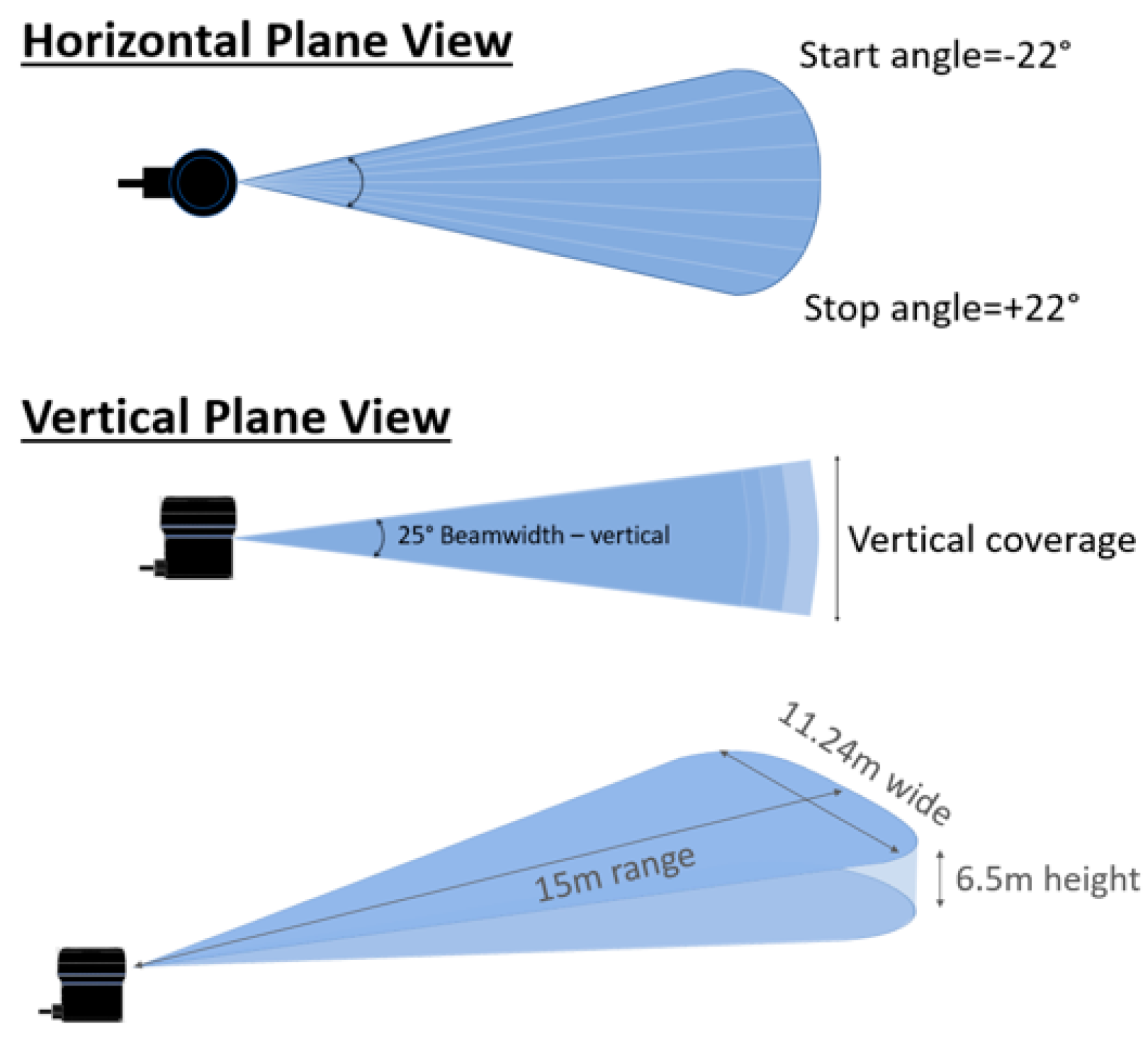
Our preliminary sensor studies revealed an acoustic sensor’s ability to observe oil droplets and an oil plume through wave tank tests [27]. Among the available sonars that can be operated on our Explorer AUV, the Ping360 scanning sonar from BlueRobotics (See Figure 2) was selected for its advantages as follows compared with other types of sonar. The Ping360 sonar head has an acoustic transducer, which continuously emits a narrow beam of acoustic pings through the water. This transducer can be mechanically rotated to a desired incremental angle (≥1°) allowing the vehicle to visualize its surroundings up to a 360° swath without having to turn the vehicle orientation itself. This is a great advantage especially for a large-sized vehicle such as the Explorer AUV as it enables rapid collection of real-time data over a wider space.

Although we set the scanning mechanism to work in the horizontal plane, the beamwidth angle (25°) of the signal expands the vertical coverage to some extent, resulting in a quasi-three-dimensional survey. Lastly, the Ping360 was a cost-effective choice because of its relatively low price compared with other sonars.

2.2.2. Target: Micro-Sized Air Bubbles

For open water experiments, we explored several options for a potential proxy that can best emulate oil droplets in seawater [27,28]. Two indispensable conditions were considered: first, it must be environmentally safe, unlike a real chemical plume; second, it must have acoustically similar characteristics to a multiphase oil plume, meaning that it should be visible by our primary sensor, the Ping360.

To satisfy both conditions, we selected air bubbles. Field trial results indicated that small air bubble plumes appeared just like discrete oil patches on the sonar images [27]. For an air bubble plume to be suspended for a sufficient length of time during the experiment, the size of the air bubbles was defined via research, which was around 100 microns in our application [28].

We investigated several methods to generate air bubbles of diameters less than 100 microns. Microbubbles have been widely studied and used in various fields including water treatment, water purification, mineral processing, natural ecology restoration, cleaning, and medicine [29,30]. Different types of microbubble generators have been developed for large-scale applications and many are commercially available. We tested bubbles generated with the Dissolved Air Flotation (DAF) bubble-generating system developed by Zedel and Butt [28,31]. The average size of the bubbles ranged between 100 and 200 microns. The collective rise velocity of the plume of bubbles was five to ten times higher than the velocity estimated for individual bubbles of the same sizes [29]. We tested another commercial off-the-shelf microbubble-generating system developed by Nikuni Japan [30]. The system uses a centrifugal pump [32] to mix and dissolve the air at a high pressure into water, thus eliminating the need for an air compressor and a large mixing tank (see Figure 3). The sizes of the bubbles vary depending on operating conditions, including air and water flow rates, pressure, and release depth. The pump system was configured to be able to operate from a vessel, creating a moving source and, in turn, a longer plume.

2.3. Real-Time Data Process

A sensor model for processing sonar data was developed consisting of a sequence of analysis modules. Whenever new measurement updates take place, each module analyzes the collected sonar data accordingly within a set of criteria. Throughout the mission, the data are processed and updated in real time.

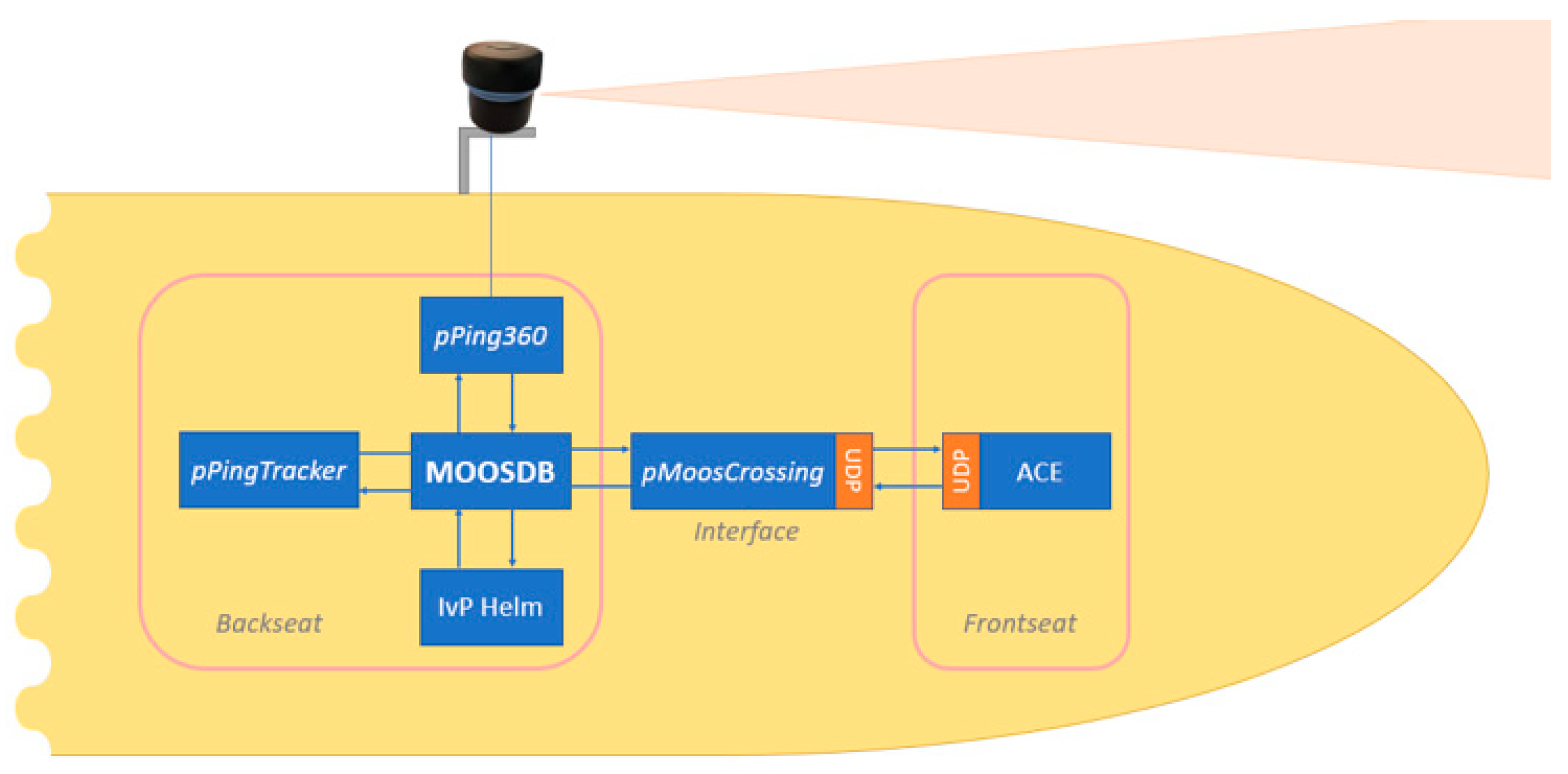
2.3.1. Onboard Computer Interface

In this section, we introduce the onboard computer interface, which involves the integration of an independent control computer, facilitating bidirectional data transfer and enabling adaptive mechanisms for underwater missions. An AUV mission file typically runs on the manufacturer’s main vehicle control computer (VCC or frontseat driver), which controls the AUV’s dynamic motions to maintain the desired vehicle state (course, speed, and depth). However, with the demand for increased autonomy in underwater missions, many AUVs nowadays have been equipped with an additional system (a backseat driver architecture) where a dedicated software environment is implemented [33]. This separation of the vehicle’s dynamics control processor (frontseat) from the intelligent control processor (backseat) can be extremely beneficial for underwater missions, which demand adaptive mechanisms. Furlong [34] explained that the primary benefit of having a separate frontseat/backseat architecture is the increased software portability because the higher-level autonomy system is decoupled from the lower-level vehicle details.

International Submarine Engineering (ISE), the AUV manufacturer, integrated an independent control computer on Memorial University’s Explorer AUV during a major vehicle upgrade in 2019. There are several available frameworks for an adaptive mission system that were specifically designed for underwater vehicles [24]. Examples include MOOS-IvP [35], ROS [36], T-REX [37], ORCA [38], and so on. Among those options, the Mission-Oriented Operating Suite (MOOS-IvP) software was implemented in our system. The pMoosCrossing application allowed bidirectional data transfer between the frontseat (ACE) and the backseat (MOOS) through the UDP protocol as shown in Figure 4. Therefore, data from various sensors on the Explorer (e.g., depth sensor, velocity sensor, altimeter, and GPS) along with data from the payload sensor (Ping360) were regularly updated to the MOOSDB so that IvP-Helm could make decisions on the desired vehicle state in the following control cycle.

2.3.2. Sonar Noise Band

The Ping360 is an active sonar, which sends a ping (a pulse of sound) and receives a reflected wave (echo) in order to detect objects. While operating, the Ping360 also generates strong noise around the sonar head presumably emanating from the transducer during its rotational motion [27]. Unlike possible ambient noises, this noise is persistent, and the thickness of the surrounding noise band is approximately 0.25 m. This means that the analysis algorithm would not be able to distinguish an object within this band. In other words, valid detection can be made only in the range outside of this proximate region. In order to eliminate unnecessary confusion in the later analysis process and keep the total data size as low as possible, any measurements obtained in this proximate region (0–0.25 m sonar range) were excluded.

2.3.3. Propagation Speed of Sonar

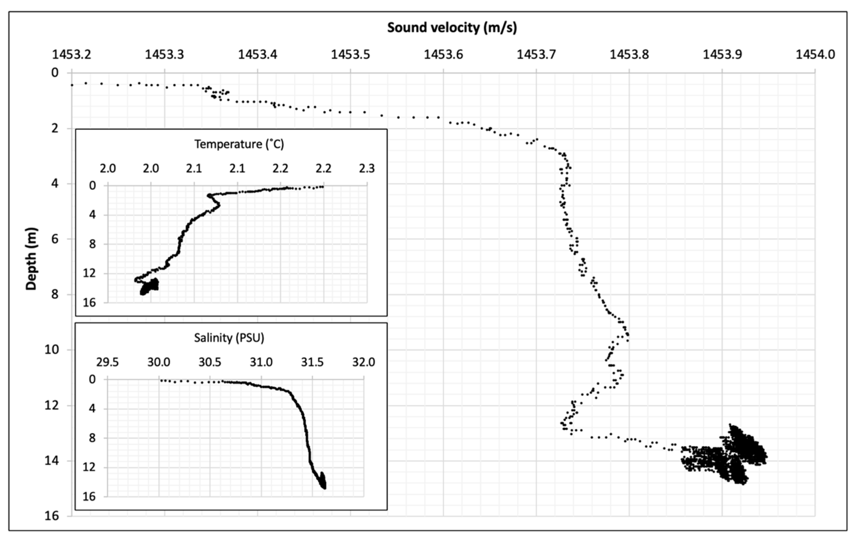
Sound travels at different speeds depending on the physical properties of the medium, while it is independent of frequency (called non-dispersive): for example, it travels at about a speed of 1500 m/s in seawater and 340 m/s in air. So, the speed of sound in a non-dispersive medium such as water is affected by oceanographic parameters such as the ambient temperature (T), salinity (S), and pressure (p) of the water [39]. As a general rule, increases of 1 °C, 100 m of depth, and 1 ppt salinity result in 3, 1.7, and 1.3 m/s increases in sound speed, respectively [40]. More empirical data on this correlation were published by Roemmich and Gilson [41].

In our system, we take into account the variability of sound speed due to changes in oceanographic parameters. We employ the formula presented in [42] and used in experiments by the authors of [43] to calculate sound speed, as shown in the following equation:

$$C\left(T,S,z\right)=1449.2+4.6T-0.055T^2+0.00029T^3+\left(1.34-0.010T\right)\left(S-35\right)+0.016z$$

(1)

where T represents temperature (°C), S represents salinity (p.s.u.), and z represents the depth of water (m). This formula provides accurate sound speed calculations up to a water depth of 400 m [44].

To ensure the precision of our system, we continuously update salinity, temperature, and depth information in real time, operating at a frequency of 1 Hz. The calculated salinity at the depth of operation is then incorporated into the sound speed formula, allowing us to accurately determine the speed of sound in the underwater environment. Figure 5 shows the sound velocity profile calculated using Equation (1). Insets show the temperature and salinity collected in the ocean in Holyrood Bay as independent variables.

With the known propagation speed of sound (C), the traveled distance of the sound (i.e., distance from the sonar head to an object where a strong acoustic signal is reflected) can be accurately calculated using the following equation:

$$d=C\times 0.5t,$$

(2)

where d is distance, C is the known speed of sound, and t is the measured time for the sound to return. This approach enables our AUV to adapt to changing conditions and effectively track plumes even in dynamic underwater settings, as we will elaborate in subsequent sections. In the following sections, we will present the method used to determine the detection threshold, which optimizes the performance of our system, as well as a novel continuity method we developed.

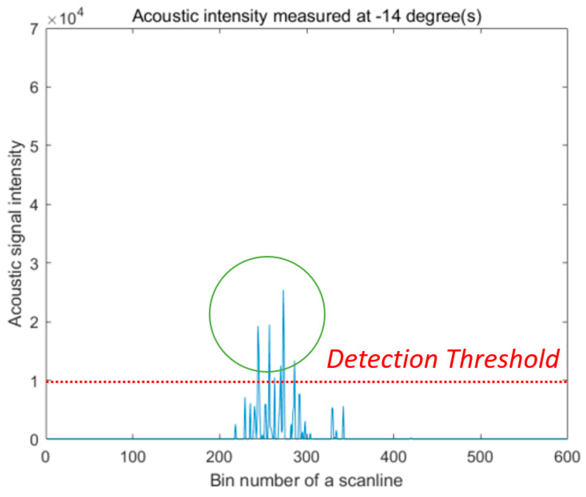
2.3.4. Detection Threshold

When a pulse of sound is emitted from the Ping360, a straight acoustic beam travels through dark (as in uncharted) water in a wave pattern at 750 kHz frequency. Similar to someone shining a flashlight in a dark room and only the space where the flashlight’s beam is reflected becoming visible, an acoustic beam (hereinafter referred to as a ‘scanline’ in this paper) illuminates the space where the oscillating wave has passed through water [44]. A reflected pulse is displayed as an individual line depicting the cross-section of an object or a surface. When there is a target located within the set range, an echo bounced off the object is displayed as a stronger acoustic signal than the ambient noise level within a scanline (see Figure 6).

A scanline of the Ping360 consists of 600 bins, equally split, which deliver a piece of acoustic information on the returned pulse in the form of an analog signal. In our analysis, the range to the detected target was calculated based on the distance to the bin, which carries a higher signal than a set detection threshold (DT) (see Figure 6). The size/length of the bin depends on the set range: for example, the bin size is 3.3 mm when the range is 2 m while it is 83.3 mm when the range is 50 m (the maximum range of the Ping360).

The acoustic strength of the returned echo is dependent on two parameters: the size of the target particles and the density (concentration of the particles) of the target [45]. A larger and denser material will reflect a stronger signal. Through preliminary tests conducted at 1~2 m depth of water targeting microbubbles as a proxy for a real oil plume, an appropriate DT was determined. The DT is a key criterion in the first analysis step. It indicates the minimum required strength of the signal for detection.

The DT was determined through systematic experimentation using a mobile bubble generator and the Ping360 sonar, as detailed in our prior article [27]. After evaluating various DT values, we found that a threshold of 10,000 acoustic intensity units provided a balance between sensitivity and specificity, enabling precise plume target recognition while minimizing false positives.

2.3.5. Stalled Continuity Method

The Continuity method is one of the automatic detection methods that have been applied in image processing [46,47]. A similar concept is also used in the saturated raw distance function of the Tangent Bug algorithm, which detects discontinuities that separate a continuity interval to define an obstacle ahead [48,49]. The continuity/discontinuity in these applications mainly identifies the border between the object and its surrounding environment. This can work well where there is a significant difference in density between the material particle and the ambient medium (i.e., air) displaying a distinctive boundary. However, a multiphase oil plume in seawater is characterized by being discontinuous, having an unevenly distributed density, and having an ambiguous boundary especially while it is dispersing. Hence, it is essential to have a second criterion to determine how to demarcate an oil patch and water from other patches. Therefore, we utilized the stalled continuity (SC) method.

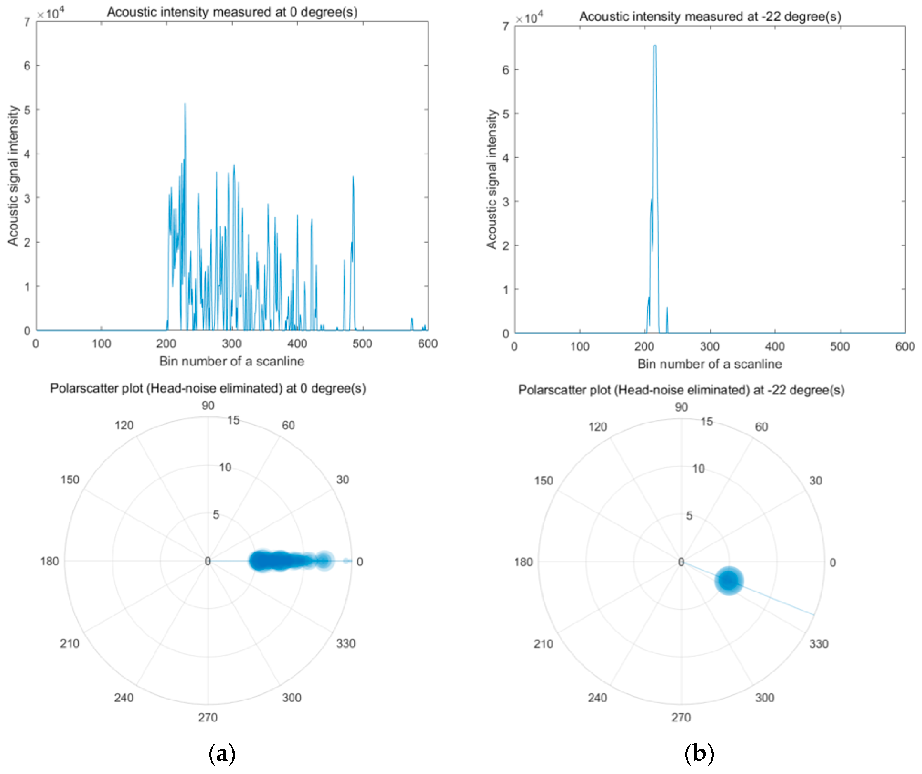
An individual oil patch can be identified by observing the number of consecutive signals passing the DT level in a scanline (see Figure 7). For example, in our setup, any detected oil patch larger than 1 m was considered as a valid oil patch of interest. So, when the required number of consecutive bins (equivalent to 1 m) shows signals above the detection threshold, continuity becomes true.

However, non-oiled spaces between small oil droplets may result in intermittent non-passed signals among the passed data, which we treated as a false discontinuity. This means that valid continuity information is repeatedly impaired; hence, we introduced a counter-counter (CC) to nullify this false discontinuity. Therefore, when discontinuity takes place, the counter-counter begins to take a count of the number of negative signals. An allowable droplet gap (AG) is another criterion used here to confirm whether it is a true discontinuity (CC > AG) or a false discontinuity (CC < AG): 0.5 m in our case. While the counter-counter is active, the continuity is stalled rather than terminated. To some extent, this helps to alleviate intricacy in discerning a multiphase oil mixture.

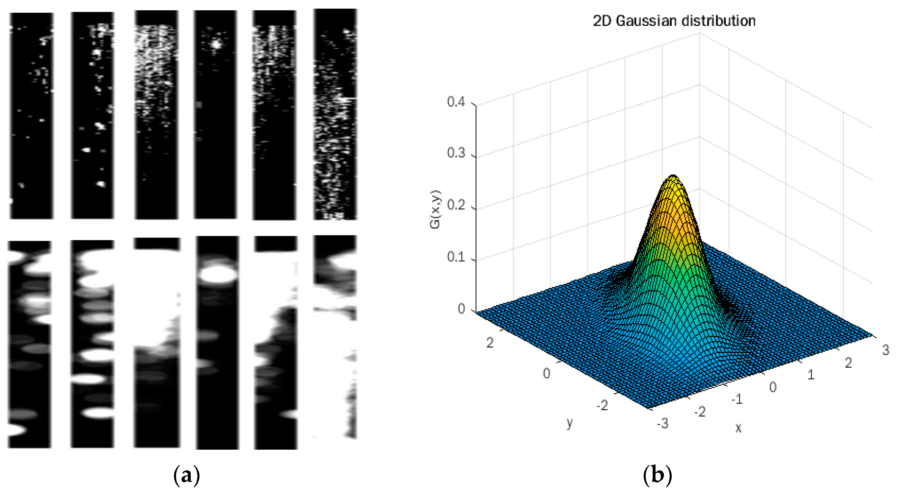
2.3.6. Gaussian Blur

In this section, we present a sonar image blurring technique for enhancing the clarity of data inputs, leading to better tracking outcomes.

The valid data that have passed the applied criteria are sent to a sector process module. This stage is a 2-dimensional areal analysis as opposed to the 1-dimensional line analysis, which was conducted in the previous stage. A set of scanline data piled up from the start angle (e.g., −22°) to the stop angle (e.g., +22°) completes a fan-shaped sonar image (see Figure 8), which makes a full azimuth angle of 44° ahead of the AUV. This complete sonar image is called a “fully scanned image”. The original time-indexed data feature somewhat scattered (noisy) data for two reasons: first, there is a difference between the observed data and real data. Some true signals might not have been reflected while some false signals might have been faultily reflected.

Second, a lot of small gaps between tiny bubbles result in sporadic signals. Then, those low signals that did not pass the DT (undetected) were excluded in the processed data. They all inevitably lead to noise-like and patchy profiles (see Figure 9). Since the scattered data are difficult group, we adopted a Gaussian blur (also known as Gaussian smoothing) method to reduce the noise. Gaussian smoothing is a type of convolution operator using a mathematical model [50] called a “2D isotropic Gaussian function” as shown in Equation (3),

$$G\left(x,y\right)=\frac{1}{2\pi {\sigma }^2}{e}^{-\frac{x^2+y^2}{2{\sigma }^2}},$$

(3)

where σ is the standard deviation of the distribution and (x, y) is the location index. The Gaussian function generates a circularly symmetric distribution, hence a bell curve shape (see Figure 9). It has been widely applied in image processing, usually in the digital editing of photos and videos [51,52,53,54]. More recently, coupled with machine learning or artificial neural networks, its application has expanded [50,55,56,57]. Like digital images constructed of pixels, a fully scanned acoustic image is also made up of numbers in a lot of cells (or kernels). Despite the disadvantage of losing fine image details through this process, the process facilitates grouping of the scattered data, which enables us to overcome the errors in the identification of small patches.

For Gaussian smoothing the control of both the kernel size and sigma was guided by a preliminary iterative process based on the raw data presented in Figure 9a. Subsequently, we maintained a constant set of coefficients (kernel size and sigma) for each sonar image throughout the mission. This decision was driven by the nature of the application, characterized by fixed parameters such as the sonar range (50 m), the number of bins (600), and the azimuth (turning) angle (44°). These constants provided stability in the plume tracking methodology and effectively bridged gaps between detected bubbles, enabling the recognition of the plume as a cohesive entity rather than a collection of individual bubbles.

2.3.7. Labeling Oil Patches

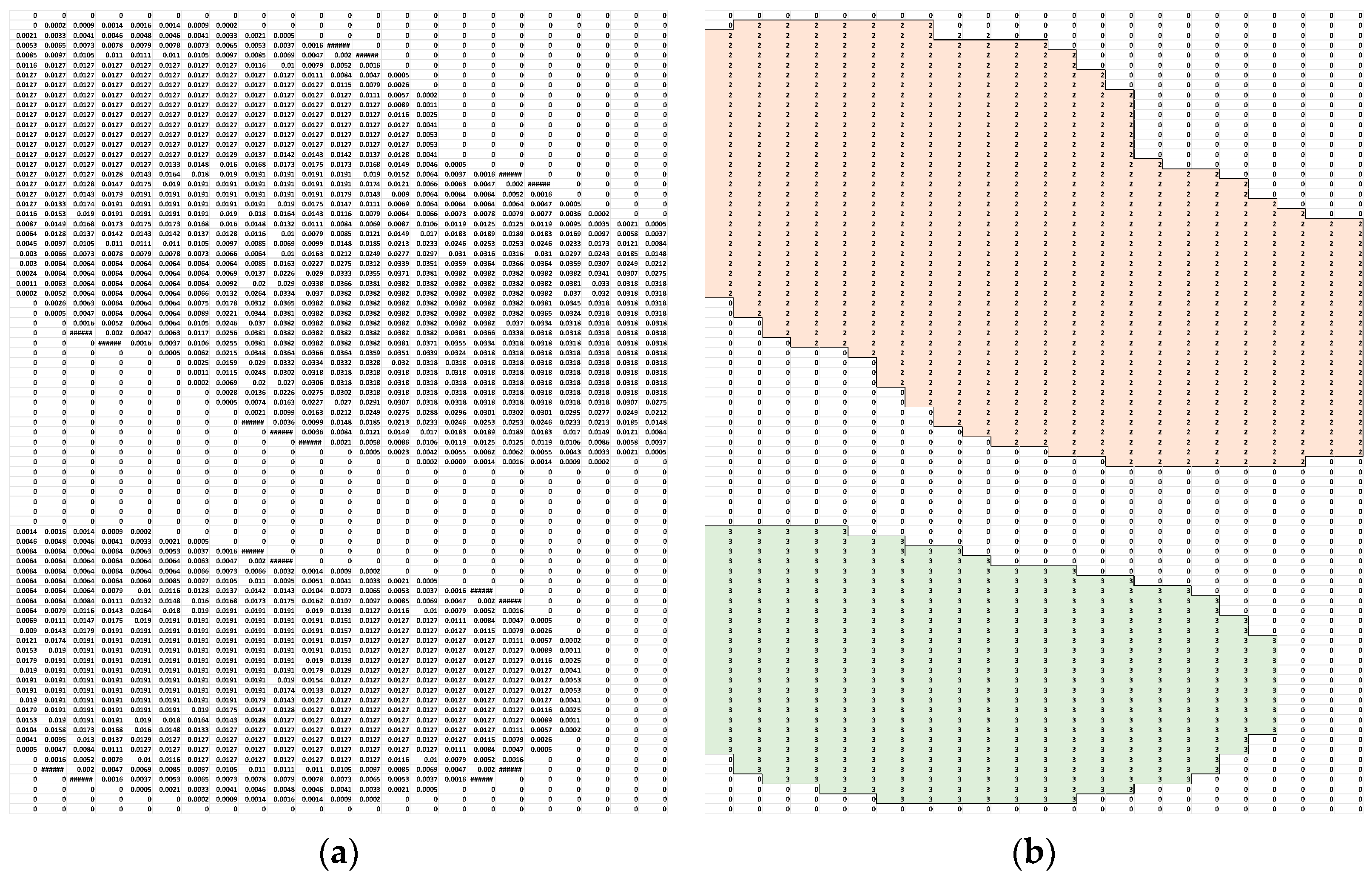
The Gaussian blurred image can be expressed as convolution kernels as shown in Figure 10a. The kernels that touch or share their edges become connected and the adjoined kernels are considered as a part of the same object if they are horizontal, vertical, or in a diagonal direction as shown in Figure 10b. Once each patch is grouped together, each clustered patch is labeled. Although the actual values in the kernel are multilevel (i.e., non-binary), all non-zero values are treated equally when being labeled.

2.3.8. Occupancy Polar Grid Mapping

Generating a map based on sensor data to understand the environment is one of the fundamental tasks in robotics [58]. The concept of the occupancy grid is to create a map of the environment as an equally spaced field of binary (random) variables, which represent the presence of an object at that location in the environment. So, usually true (1) means that an object occupies the location, and false (0) represents an empty space. In comparison, when adding the concept of probability, each occupied cell holds a probability value instead of a binary value (1 or 0). The occupancy grid method has become popular through the work of Moravec and Elfes [59]; then map building using occupancy grids was improved by Konolige [60]; and more recently, metrical mapping work was conducted by Thrun [61], who enhanced the accuracy of the grid map.

The fundamental assumption of occupancy grid mapping is that the environment map is constructed, as the vehicle pose is known and the location of the detected object is static. As we disregard the density of our target (plume) in our paper and the plume is considered to be dynamically dispersing (non-static), the acquired information of the map is only taken into account as a temporal view of the world. So, the total percentage of the occupied cells within the cone-shaped binary kernels is the key criterion to determine the next desired pose of the vehicle (see Figure 11). The occupied cells in red represent the detected plume within the fully scanned sector.

We established an AUV turning angle in accordance with the percentage of the total occupied cells as determined below, so that the vehicle can follow the edge of the plume while still maintaining a certain distance from the plume:

$$y=\frac{\max \left(turningrange\right)}{stepsize}occupancy,$$

(4)

where occupancy is the difference between the average of the full (60%) and empty (0%) percentage and the percentage of the total occupied cells; control turning ranges (±10.0°); and control step size is 60.

3. System Design

In this section, we will delve into the comprehensive system design, providing a detailed overview of its architecture and functionality. Our objective is to present a clear and concise representation of the system’s underlying structure and operation through the incorporation of well-structured pseudocode. Additionally, visual aids in the form of diagrams will be included to aid in visualizing and understanding the system’s components and their interactions. By combining these elements, we aim to offer readers a comprehensive understanding of the system’s design and implementation, facilitating a deeper comprehension of its capabilities and potential implications.

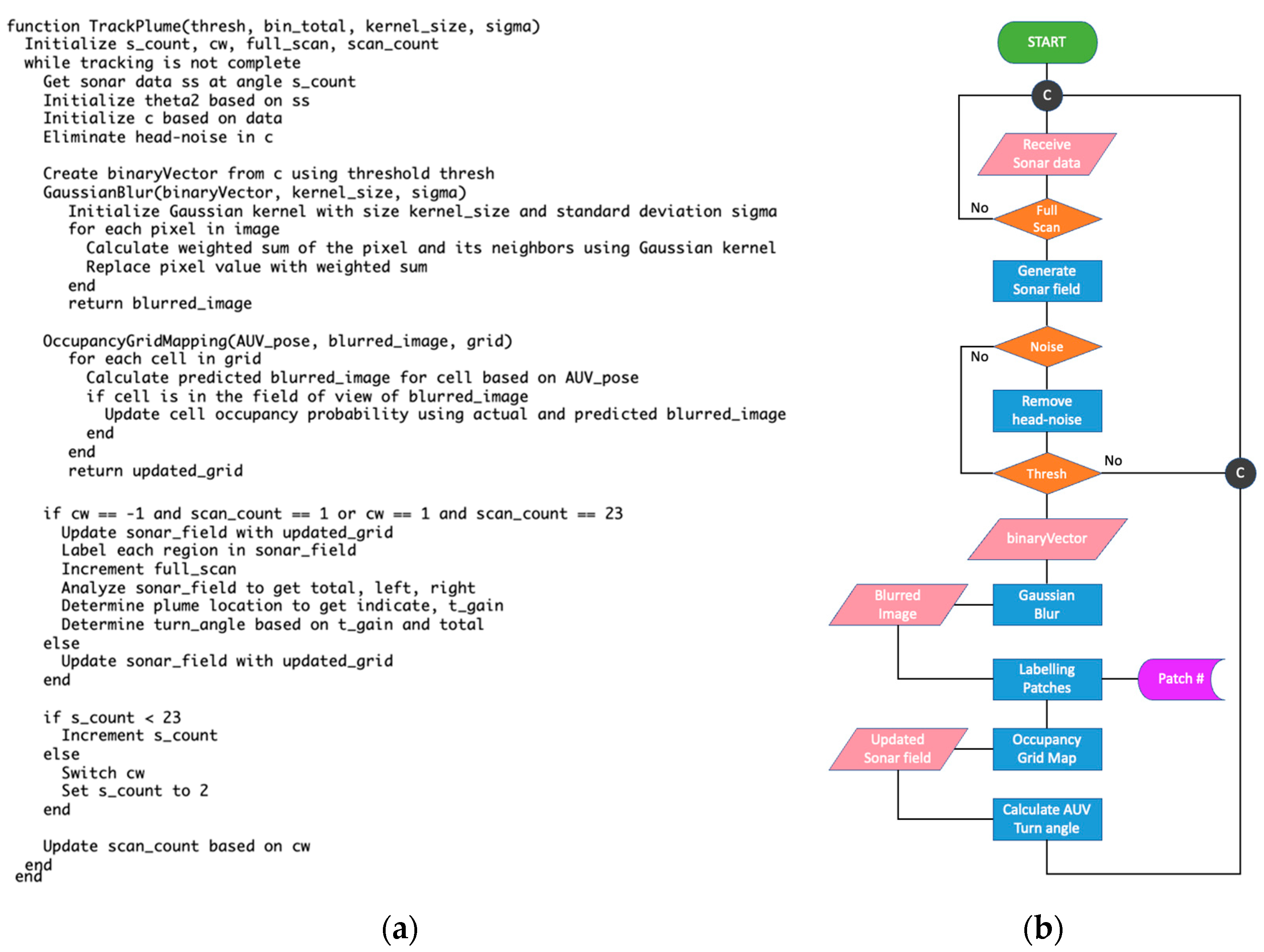
The following Figure 12a is the pseudocode of our system described in the previous section. This pseudocode represents a loop that continuously gathers and processes sonar data to track an underwater plume. After creating a binary vector from the sonar data using a threshold, we apply Gaussian blurring to reduce noise and detail in the data. Subsequently, we perform occupancy grid mapping to represent the AUV’s environment. The algorithm then proceeds with the labeling, analysis, and decision-making steps as previously described. It is important to note that this pseudocode serves as a simplification and may not include all the details required for an actual implementation. Proper initialization of parameters, such as thresh, bin_total, s_count, cw, full_scan, scan_count, kernel_size, sigma, and updated_grid are necessary. Additionally, specific functions like sonar_field, GaussianBlur, OccupancyGridMapping, turn_angle, and t_gain should be defined in the actual implementation. Figure 12b presents a comprehensive view of our system design, which is a culmination of various components working together to achieve a specific goal. This loop diagram illustrates the iterative process of the plume tracking algorithm. The loop begins with data acquisition from the sonar sensors and continues through various stages. Overall, the system is designed around the principles of ‘Sense, Analyze, and Reaction’, enabling it to adapt to real-time data and make autonomous decisions.

4. Field Experiment

The field experiment was conducted with the Memorial University Explorer survey-class AUV from October 2022 to February 2023 in Holyrood Bay, which serves as the marine base of the university. The sheltered bay provides water depths ranging from around 10 to 50 m for the experiment. The detailed experimental setup and trial results are described in the following sections.

4.1. Experimental Setup

The developed tracking module (named pPlumeTracker) was implemented on MOOS, and the backseat driver computer on the Explorer AUV. The AUV was launched through a slipway near the AUV workshop. To create a plume, the bubble generator was strategically positioned on the edge of the dock. The generated bubble was released from the bubble outlet (100 m off the dock) through the extended pipe. The experimental site on the map is shown in Figure 13.

The decision to place the plume on the port side of the AUV deserves further elucidation. The location of the plume was a result of careful consideration of several factors. Notably, the bubble generator’s installation site, fixed on the dock, introduced constraints on the plume’s proximity to the harbor. Given the limited length of the pipeline connected to the generator, the bubble plume had to be generated in relatively close proximity to the harbor wall. To ensure the AUV’s safety and alignment with its designated heading, we decided to position the plume on the port side of the vehicle. This configuration allowed for controlled and safe passage of the AUV while the plume was situated to the left of its trajectory.

The selection of the scanning parameters, including the 44° azimuth angle and 50 m range, was made after careful consideration of the trade-offs between scanning parameters, mission objectives, and the AUV’s cruising speed [27]. This configuration resulted in a 12 s duration for a single scan of 44°, during which the AUV would travel approximately 18 m. This setup was optimized for the specific experiment, taking into account the expected size of the target plume, mission goals, and the need for real-time responsiveness. The data and analysis guiding this decision can be found in our previous publication [27]. This configuration allowed us to effectively track the target plume within the experiment’s scope.

4.2. Experimental Result

The sonar images collected from the Ping360 against the microbubble plume are presented in this section and the virtual tracking performance by the pPlumeTracker module of the backseat driver is discussed.

The primary objective of this field trial was to confirm the function and operation of the module, pPlumeTracker, developed based on the proposed detection method. While conducting consecutive line-following missions, the Ping360 continued to capture the micro-sized bubble plume for about 270 s (4.5 min) as shown in Figure 14. Each full scan took approximately 12 s to complete each fan-shaped sonar screen.

The AUV trajectory recorded in the local frame of reference (local Cartesian coordinates) by the backseat driver is plotted in Figure 15. The approximate location of the plume relative to the AUV path is presented (not to scale). There were two significant (high peaks: marked as A and B) and one suspected (low peak: marked as C) moments where the microbubble plume appeared on the sonar screen and was confirmed by the pPlumeTracker module. The pPlumeTracker module response during the mission is shown in Figure 16. The total detection result (one of the main outcomes from pPlumeTracker) indicated that the highest detection was 2669 while the background average was about 1515. We only generated the turning commands within the local module instead of parsing them as the real vehicle driving commands to the backseat drive system, for the sake of the vehicle safety at this stage. Hence, these presented commands were all virtual. The virtual turning command from the pPlumeTracker module remained between −9.5° and −10.0° (see Figure 16), which was not ideal since it would lead to a continuous turning. Considering the turning angle ranges being between −10.0° and +10.0°, the result revealed that the set background threshold was too high, which impacted the turning commands in a way that the vehicle was (virtually) directed to turn to the port side. Therefore, the guiding threshold to determine the presence of the plume was re-set to the average (1515). Also, the maximum turning angles were increased to the range between −20.0° and +20.0°. After those coefficients were tuned, the data were replotted as shown in Figure 17. The tuning process produced a more optimized command result.

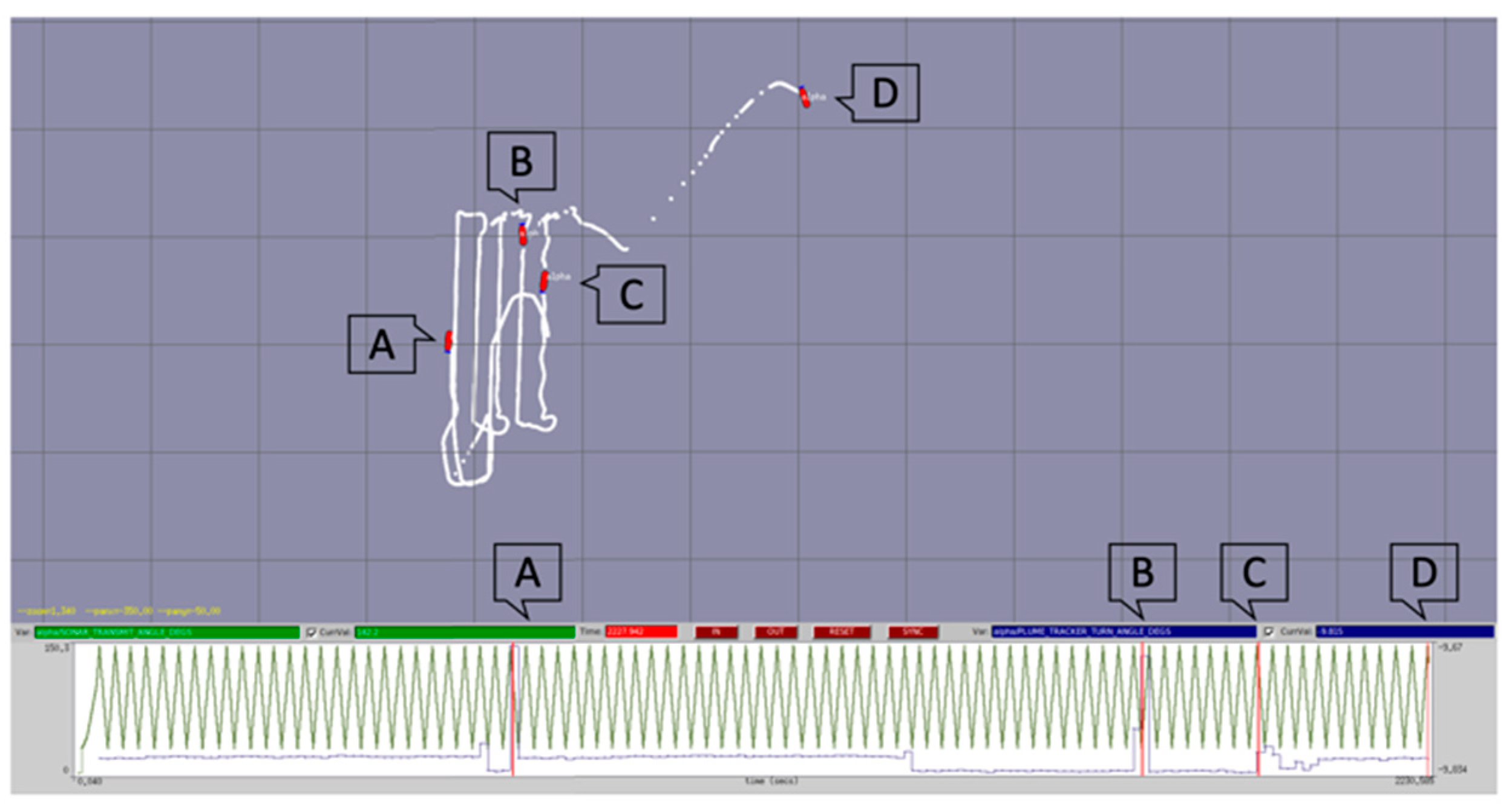
5. Discussion

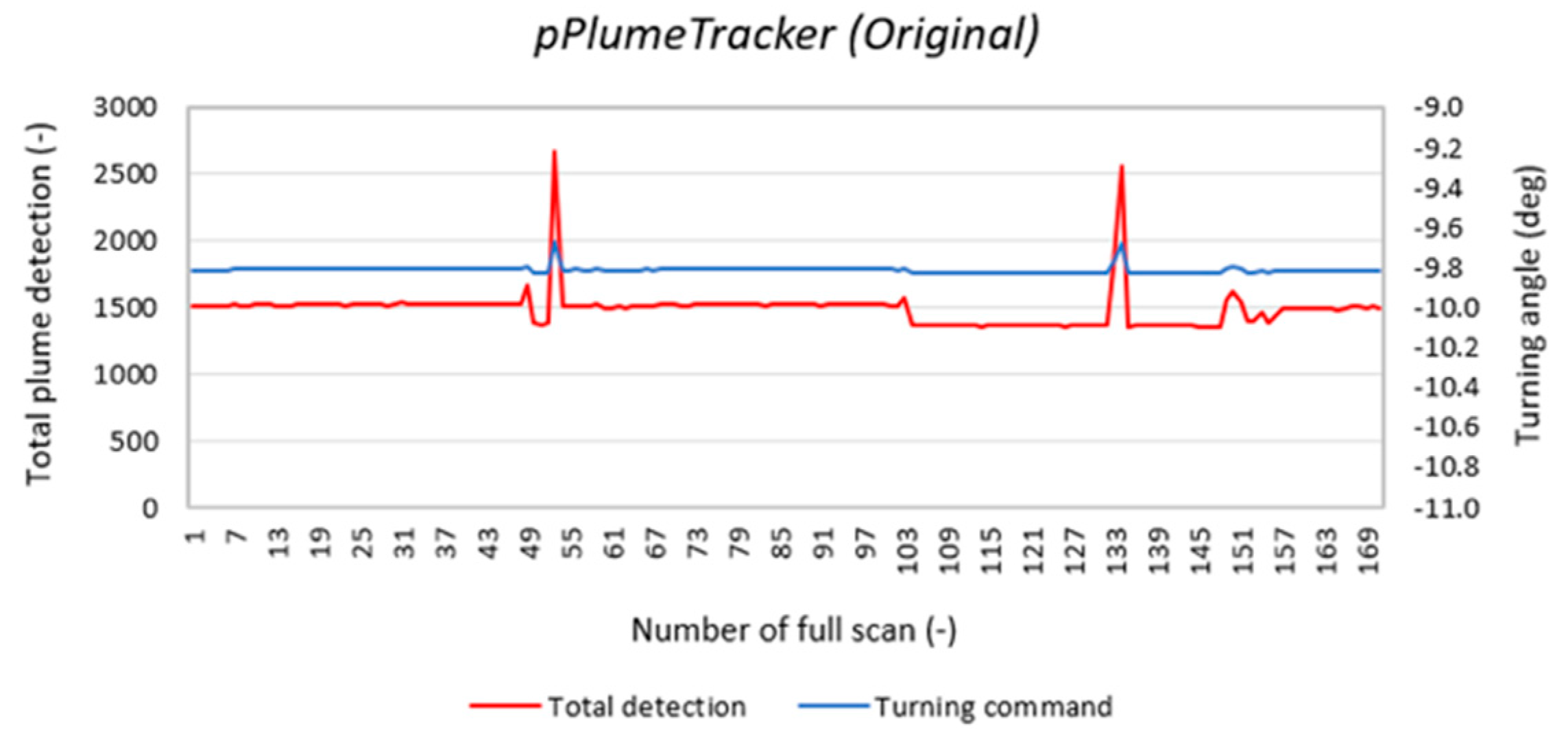
The MOOS plume tracking algorithm worked successfully during the mission, confirming the presence of the plume. In this trial using the real vehicle in open water, the adaptive component was conducted virtually by making the “heading command” mute to the vehicle-driving computer, allowing further tuning with pPlumeTracker. Two variables were tuned during the post-processing step, thus improving the output of the pPlumeTracker.

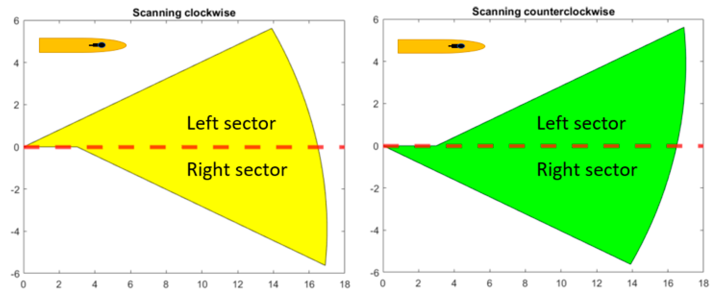
The Ping360 is a “3D scanning sonar” with a mechanically rotating transducer inside the sonar head. This rotating action causes a delay between each beam of the scan of up to 35 s. For example, if the sonar completes the full scan (360°) with an incremental angle of 1° while the vehicle keeps moving forward at its cruise speed (1.5 m/s), the complete scanned coverage is not a circle, but rather an oblong shape. This distortion of the sonar coverage can be minimized when the sonar is set to scan the forward section from the vehicle only (see Figure 18). The sensing coverage and the time delay are traded off against each other. Hence, to minimize the delayed time and to maximize the areal coverage, it is crucial to find the most optimal setup: incremental angle (1° or 2°), sonar range (20–50 m), and total scanning azimuth (fan-shape or full scan).

The developed method encompasses four key contributions that enhance the AUV’s capabilities in detecting and tracking oil plumes in complex underwater environments. First, the implementation of the stalled continuity (SC) method enables the precise identification and demarcation of individual oil patches within the multiphase oil plume. The introduction of the counter-counter (CC) mechanism effectively addresses intermittent non-passed signals, ensuring the preservation of valid continuity information. Second, the adoption of Gaussian blur in a 2-dimensional areal analysis significantly reduces noise and enhances data coherence in fully scanned acoustic images. This approach successfully overcomes the challenges of scattered and noisy data, improving the accuracy in identifying small patches. Third, the approach to labeling oil patches enhances the AUV’s ability to recognize oil plumes by providing crucial contextual information. With the labeled patches, the AUV’s detection algorithms make more accurate and informed decisions, resulting in improved detection sensitivity. Finally, the incorporation of occupancy polar grid mapping, with probability values for occupied cells, allows for a temporal view of the world. Utilizing the percentage of occupied cells within cone-shaped binary kernels, an AUV turning angle was established to follow the plume’s edge while maintaining a safe distance, enabling effective plume tracking in our missions.

6. Conclusions

In this study, our contribution is to present a comprehensive algorithm that integrates a payload sensor, identifies micro-sized air bubbles as targets, and employs advanced real-time data processing techniques. The design principles and methodologies were found to improve the accuracy and effectiveness of oil patch tracking, thereby contributing to the field of environmental monitoring and pollution control.

During ocean field trials, we developed and tested an adaptive algorithm using a MOOS plume tracking algorithm and the Ping360 sonar for detecting and tracking an underwater plume. This study successfully demonstrated the use of bubbles as a proxy for plume tracking, demonstrating an effective approach for remote detection of an underwater oil plume. The results of the experiment indicated that the MOOS plume tracking algorithm was able to successfully respond to the bubble plume and confirm its presence. The utilization of sonar, particularly the Ping360, was also shown to be effective in detecting the plume and providing real-time data during the mission.

The work highlighted the importance of the backseat driver approach in plume tracking. This approach showed that our developed pPlumeTracker algorithm was able to effectively generate the heading commands and enable the AUV to respond to the plume in real time in an adaptive mission.

Overall, the results of this study demonstrate successful implementation of a backseat driver approach for the remote detection of an underwater oil plume using bubbles as a proxy and sonar as a detection tool on a survey-class AUV.