Article

Analytical Framework for Sensing Requirements Definition in Non-Cooperative UAS Sense and Avoid

by
Giancarmine Fasano
* and
Roberto Opromolla
Department of Industrial Engineering, University of Naples Federico II, 80125 Naples, NA, Italy
*
Author to whom correspondence should be addressed.
Drones 2023, 7(10), 621; https://doi.org/10.3390/drones7100621
Submission received: 28 August 2023 / Revised: 27 September 2023 / Accepted: 28 September 2023 / Published: 3 October 2023
(This article belongs to the Special Issue Next Generation of Unmanned Aircraft Systems and Services)

Abstract

:
This paper provides an analytical framework to address the definition of sensing requirements in non-cooperative UAS sense and avoid. The generality of the approach makes it useful for the exploration of sensor design and selection trade-offs, for the definition of tailored and adaptive sensing strategies, and for the evaluation of the potential of given sensing architectures, also concerning their interface to airspace rules and traffic characteristics. The framework comprises a set of analytical relations covering the following technical aspects: field of view and surveillance rate requirements in azimuth and elevation; the link between sensing accuracy and closest point of approach estimates, expressed though approximated derivatives valid in near-collision conditions; the diverse (but interconnected) effects of sensing accuracy and detection range on the probabilities of missed and false conflict detections. A key idea consists of focusing on a specific target time to closest point of approach at obstacle declaration as the key driver for sensing system design and tuning, which allows accounting for the variability of conflict conditions within the aircraft field of regard. Numerical analyses complement the analytical developments to demonstrate their statistical consistency and to show quantitative examples of the variation of sensing performance as a function of the conflict geometry, as well as highlighting potential implications of the derived concepts. The developed framework can potentially be used to support holistic approaches and evaluations in different scenarios, including the very low-altitude urban airspace.

1. Introduction

Sense and Avoid (SAA), also known as Detect and Avoid (DAA), is a key research area for the scientific community devoted to Unmanned Aircraft Systems (UAS) [1,2], as it constitutes one of the main roadblocks to the integration of UAS operations by aviation authorities around the world. Since the first studies, SAA has been considered as a multi-dimensional problem, due to the variety of UAS categories and the diversity of airspace classes they can fly through.
Many efforts in the past concentrated on medium-size and large-size UAS flying in the traditional Air Traffic Management (ATM) ecosystem with other manned and unmanned aircraft [3,4], starting from the concept of “equivalent level of safety” with respect to manned aviation. Hence, SAA in ATM has been characterized by a well-defined framework in terms of flight rules and separation minima, with the main challenges for non-cooperative sensing being related to high closing speeds and the fulfillment of the required safety levels.
On the contrary, within the UAS Traffic Management (UTM)/U-Space ecosystem, low-altitude SAA represents a relatively recent field of activity. In fact, UTM/U-Space concepts and rules constitute themselves an open area of investigation, with many researchers currently focusing on the definition of the airspace structure, on the design of the infrastructure supporting safe and autonomous flight operations, and on the consequent needs in terms of Communication, Navigation, and Surveillance (CNS) [5,6]. Thus, recent research on low-altitude SAA is relevant not only to small UAS, for which near-term objectives involve enabling Beyond Visual Line of Sight operations, but also to Urban Air Mobility (UAM) vehicles, i.e., new entrants in UTM/U-Space scenarios, whose mission profiles can include both traditional and low-altitude airspace.
The low-altitude SAA context presents several active research topics, such as the definition of the relation among cooperative SAA, non-cooperative SAA, and infrastructure-based separation management. This lack of definition also applies to sensing requirements, safety levels, flight rules, and their links (the idea of “equivalent level of safety” is not immediately applicable), while aircraft with different flight capabilities (e.g., vertical takeoff and landing fixed-wing configurations, conventional fixed-wing systems, multi-rotors) are encountered. In this respect, the introduction of a multi-layered conflict management architecture (conceptually similar to what is applied in the ATM context) is broadly deemed to be a valuable solution [5]. Specifically, it consists of the integration of strategic path planning and deconfliction, tactical conflict management, and SAA, as different safety measures applicable in different time-to-collision intervals. Non-cooperative collision avoidance represents the last safety layer, being typically associated with a time to collision of the order of a few tens of seconds, at most. The development of such functionality faces several challenges due to the complexity of low-altitude environments (characterized by the presence of both fixed and mobile obstacles), the constrained size, weight, and power budgets of flight platforms like small UAS, and the low detectability of small aircraft flying relatively close to the ground.
In this framework, active lines of research involve the definition of sensing requirements [7], the development of ad-hoc obstacle detection and tracking techniques including data fusion [8,9,10], the derivation of effective conflict detection criteria [1], which can also be linked to recent developments in conflict probability estimation methods [11,12], the design of new sensors with low Size, Weight, and Power budgets [13], the assessment of risk, and the evaluation of separation minima [14]. These aspects are, indeed, tightly interconnected. For instance, sensing performance for conflict detection and avoidance is heavily impacted by sensor specifications and algorithmic choices, but also by the operating scenario in terms of rules and traffic characteristics.
This paper aims to offer a contribution to the definition of sensing requirements for non-cooperative airborne SAA, focusing on moving obstacles. The adopted approach is general and can thus be potentially exploited to evaluate minimum sensing requirements in different scenarios, including the open framework of low-altitude airspace. The determination of required surveillance parameters can be addressed with different strategies. A possible approach consists of using high-fidelity sample-based simulations which are characterized by a significant computational burden and require a long time for the analysis. This approach typically includes optimization techniques [15] and takes advantage of the availability of statistical models of mid-air encounters, derived from large datasets of historical data based on ground radars and, more recently, on Automatic Dependent Surveillance–Broadcast (ADS-B) [16,17]. Sample-based techniques can be used to validate given sensing architectures and to estimate performance sensitivity to given parameters. While progress is being made in the development of encounter models at very low altitudes [18], it is clear that the absence of historical datasets poses challenges for sample-based approaches, also because scenarios and procedures involving UAM aircraft are still being defined in detail.
A different strategy consists of exploiting analytical or semi-analytical tools that explore the design possibilities adopting some approximations. For instance, analytical approximations were used in [19] to analyze the results of flight experiments with radar/optical sensors and to discuss the effects of angular rate uncertainties on the estimation of the distance at the Closest Point of Approach (CPA). Approximate analytical formulas were used also in [20] to map surveillance requirements for collision risk, assuming a constant range and considering (as in [19]) only the effects of angular rate uncertainties. Numerical analyses based on first-order approximations were exploited in [7] to link sensing accuracy with SAA performance. In all these recent works, only sensing accuracy was accounted for, without considering how the probability of obstacle detection and declaration depends on range (i.e., the analyses were carried out below an assumed detection range).
Within this framework, this paper proposes an analytical approach to the definition of sensing requirements, following the line of reasoning of previous analyses on conflict detection and on the definition of adaptive sensing strategies presented in [21,22,23]. Compared with the recent literature, the main innovations lie in the fact that analytical expansions relevant to near-collision conditions are used and an integrated approach is presented, wherein the diverse but interconnected effects of different sensing requirements such as detection range and tracking accuracy are considered together with factors and constraints such as aircraft speeds and flight rules/constraints, thus encouraging the perspective of sensor-aware flight envelopes [24]. This approach can capture the stochastic nature of non-cooperative obstacle detection and declaration. Moreover, the analysis is focused on the time to closest point of approach (tCPA) as a key parameter for sensing system design and tuning. In fact, tCPA defines the available time for collision avoidance maneuvering, and a minimum value can be set based on aircraft maneuverability limits and/or other constraints (e.g., maximum allowed accelerations). Indeed, the idea of targeting specific values of tCPA also naturally drives towards space/time adaptive sensing concepts. These concepts were preliminarily introduced in [23] with reference to specific cases. In this work, the general mathematical framework supporting these approaches is presented in detail.
The innovative contributions of this work can be summarized through the following points:
  • Definition of field of view and surveillance rate requirements in azimuth and elevation as a function of the aircraft speeds and eventual trajectory constraints;
  • Derivation of the sensitivity of closest point of approach estimates on sensing accuracy parameters, expressed though approximated derivatives;
  • Evaluation of the dependency of missed and false conflict detection probabilities on sensing accuracy and declaration range, for different conflict geometries;
  • Validation of the above theoretical derivations through ad hoc numerical simulations.
The paper is structured in the following way. The methodology for the definition of integrated sensing requirements is addressed in Section 2. Specifically, Field-of-View (FOV)-related effects are analyzed in Section 2.1, based on the variation of conflict parameters as a function of speed and flight constraints. Section 2.2 focuses on the effects of sensing accuracy, which are addressed based on analytical approximations that are valid in near-collision conditions. These aspects are then combined in Section 2.3 within a probability-oriented analysis aimed at evaluating conflict detection performance. Then, Section 3 presents numerical analyses within an ad-hoc simulation environment, which allows for verifying the consistency of analytical approximations; also, it discusses the variation of conflict detection performance as a function of the conflict geometry, introducing the idea of heterogeneous sensing architectures as a possible outcome of the analysis. Conclusions are finally drawn in Section 4.

2. Methodology for Integrated SAA Requirements Definition

The main requirements that the design of SAA systems must satisfy are related to the capability to detect and track obstacles, estimate the associated collision risk, and, if necessary, perform adequate avoidance maneuvers. Basic sensing requirements [1] include the minimum detection range of obstacles, the FOV to be monitored, the sensing accuracy, measurement rates and latencies, and integrity. From a different perspective, these can be viewed as the main specifications of the cooperative/non-cooperative sensors in view of SAA applications. Several studies in the open literature are focused on detection range requirements (e.g., [1,25]). Within a worst-case perspective, these requirements are often evaluated in frontal scenarios which minimize the time to collision for a given range to the obstacles. The different requirements/specifications are strongly linked to one another. For instance, refs. [1,26] show how minimum detection range requirements are relaxed when non-frontal encounters are considered. With the same conceptual approach, this section provides analytical instruments to identify functional dependencies between other aspects, such as FOV, measurement rate, probability of detection as a function of obstacle range, and sensing accuracy.

2.1. Field of View-Related Effects and Constraints
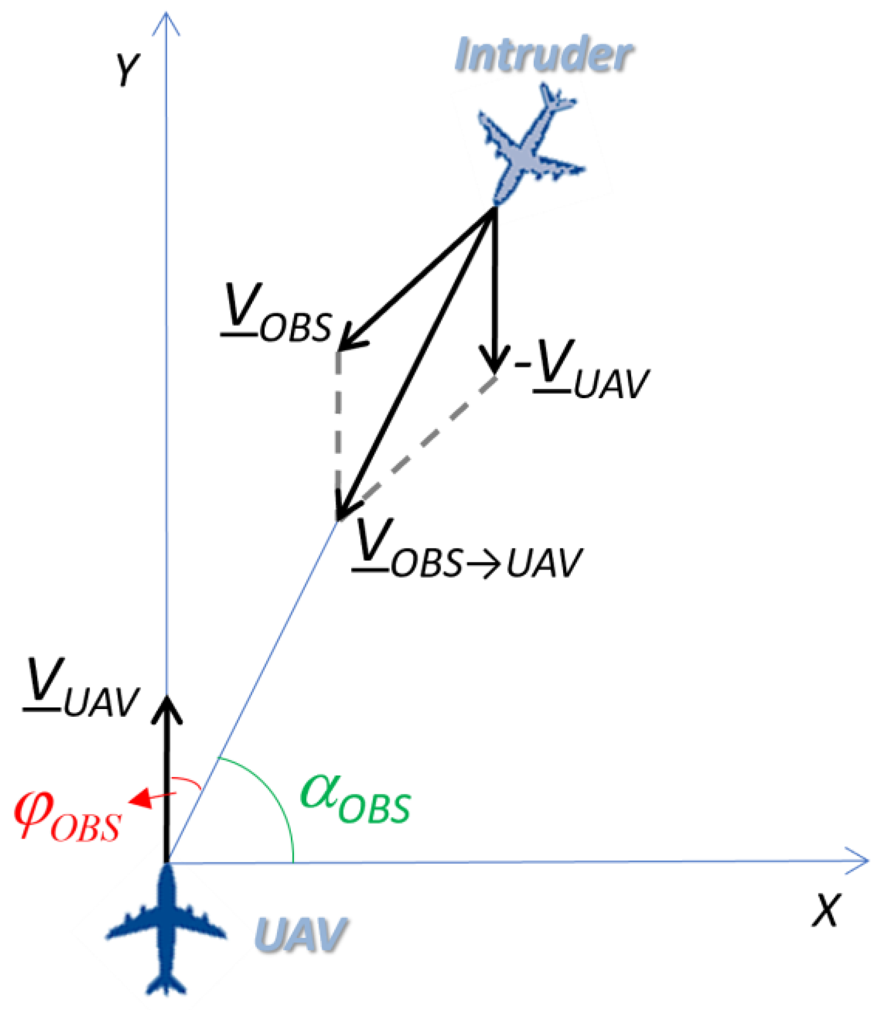
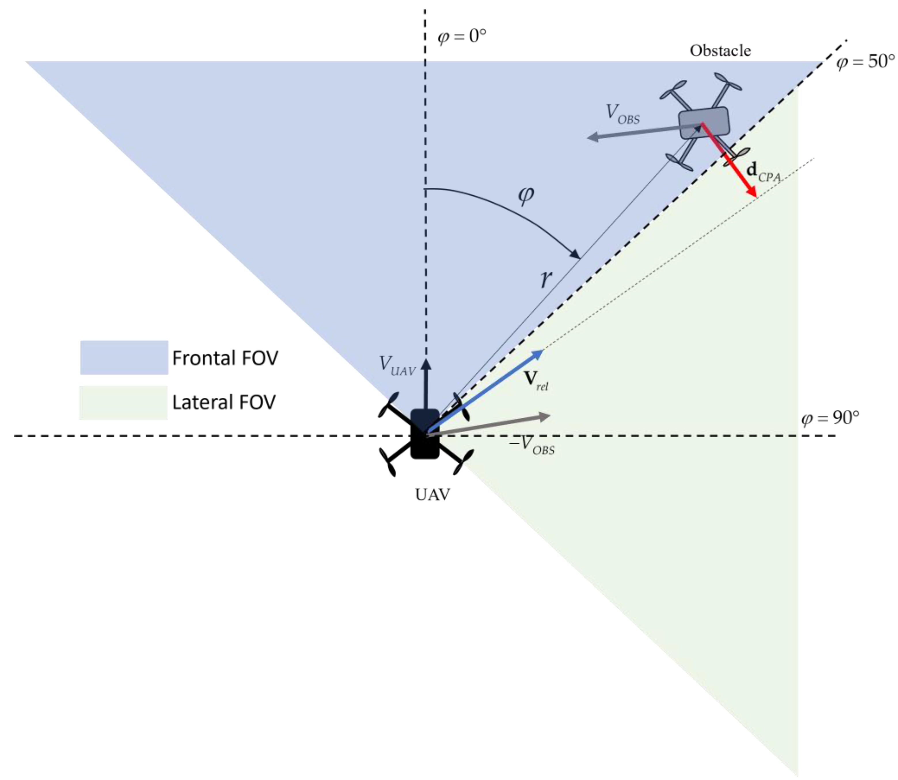
An important characteristic of a non-cooperative obstacle sensing system is its FOV, i.e., the solid angle where obstacles must be looked for. In the first SAA studies [27,28], the concept of an angular FOV similar to the cockpit of manned aircraft (220° in azimuth per 30° in elevation, due to rules on overtaking traffic) was derived from the idea of ensuring an equivalent level of safety with respect to manned aircraft. However, an FOV that has the same shape as that of manned aircraft does not imply the same level of safety, and this approach is not directly applicable in new scenarios such as UTM/UAM ones. It is thus important to analyze the actual distribution of collision conditions in the FOV as a function of the scenario. As will be made clearer in the following, this may significantly impact the technological aspects of the problem, e.g., suggesting the adoption of different surveillance rates in different areas in order to keep a constant ratio with time to collision.
An analytical methodology to study this problem is now presented. Without losing generality, it is assumed that obstacle detection sensors are aligned with the ownship velocity vector. In this discussion, the relative motion between an Unmanned Aerial Vehicle (UAV) and an obstacle in the horizontal and vertical planes are treated separately as in [20], thus obtaining different requirements on the FOV in azimuth and elevation, respectively. This is mainly derived from the idea that different constraints are likely to impact horizontal and vertical motion.

2.1.1. Azimuth

First, let us consider the 2D (horizontal) collision geometry in Figure 1, where X and Y are the axes of a reference frame with the origin at the initial position of the UAV. In particular, the Y axis is assumed to be aligned with the UAV velocity vector (VUAV).
The absolute velocity of the obstacle (also indicated as intruder in the following) and its relative velocity with respect to the UAV are indicated by VOBS and VOBS→UAV, respectively. Given this configuration, in the condition of a “real” collision (i.e., the minimum distance between the intruder and the UAV is equal to zero), the following equation holds
V O B S U A V , Y V O B S U A V , X = y O B S x O B S
where (xOBS, yOBS) is the intruder position, while VOBS→UAV,X and VOBS→UAV,Y are its relative velocity components. Equation (1) is indeed also verified in the case of an intruder flying away from the UAV (positive range rate), which, however, does not affect the generality of this derivation. The ratio at the right-hand side of (1) is the trigonometric tangent of αOBS, i.e., the angle complementary to the obstacle azimuth computed with respect to the UAV velocity vector (φOBS). Of course, Equation (1) is valid for the case of non-frontal collisions (i.e., xOBS ≠ 0). Indeed, the degenerate case of frontal encounters (αOBS = 90°), which occurs if VOBS→UAV,X = 0, is not relevant to the aim of this mathematical derivation.
Considering the geometry of Figure 1, the relative velocity components are given by the following relation
V O B S U A V , Y = V O B S , Y V U A V
V O B S U A V , X = V O B S , X
If (2) and (3) are substituted within the square of (1), and considering the definition of αOBS, the following relation can be written.
V O B S , Y 2 2 V U A V V O B S , Y + V U A V 2 tan 2 α O B S V O B S , X 2 = 0
By adding and subtracting the term “tan2(αOBS) VOBS,Y2” to the left-hand side of (4), and since, by definition, VOBS,X2 + VOBS,Y2 = VOBS2, a second-order equation in VOBS,Y can be written,
1 + tan 2 α O B S 2 V U A V V O B S , Y + V U A V 2 tan 2 α O B S V O B S 2 = 0
whose solution is given by
V U A V ± V U A V 2 1 + tan 2 α O B S V U A V 2 V O B S 2 tan 2 α O B S 1 + tan 2 α O B S
In general, to obtain real solutions for VOBS,Y, the argument of the square root in (6) must be greater than (or, at least, equal to) zero. This constraint results in a collision condition that relates the obstacle azimuth with the ratio between the UAV and obstacle velocities.
tan 2 α O B S V U A V V O B S 2 1
The immediate and intuitive meaning of (7) is that if the UAV moves slower than the obstacle, collisions will occur at any obstacle azimuth. Instead, for a UAV moving faster than the obstacle, collision conditions can be generated only if (8) holds.
tan α O B S V U A V V O B S 2 1
Recalling that, by definition, φOBS = 90° − αOBS, and since the ratio between VOBS and VUAV is denoted by k, the maximum value of the obstacle azimuth (φOBS_MAX) that can generate a collision for k < 1 can thus be computed using (9).
φ O B S _ M A X = arctan k 2 1 k 2
The trend of φOBS_MAX as a function of k is shown in Figure 2. Clearly, the faster the UAV is with respect to the obstacle, the smaller the horizontal FOV to be monitored becomes. It is also clear that the problem is symmetrical with respect to the Y-axis; hence, the analysis is limited to positive azimuth angles only.
Of course, the FOV reduction is not applicable if obstacles are faster than the UAV (k > 1). In such a case, though collision conditions can be generated at any azimuth angle, it is interesting to investigate the dependence on the azimuth of time to collision (ttc) for a given obstacle range. In fact, this suggests the possibility of exploiting different surveillance rates in different portions of the horizontal FOV. With reference to the geometry of Figure 1, ttc can be evaluated at range R as follows.
t t c = R V O B S U A V = y O B S 2 + x O B S 2 V O B S , X 2 + V U A V 2 + V O B S , Y 2 2 V U A V V O B S , Y = y O B S 2 + x O B S 2 V O B S 2 + V U A V 2 2 V U A V V O B S , Y
The functional dependency between ttc and the obstacle position in the horizontal FOV (αOBS) can be highlighted by substituting (6) within (10) and using the ‘-’ sign which either corresponds to the only real solution with negative range rate or to the one with largest range rate absolute value. Specifically, if k > 1, the maximum ttc (ttcmax) is obtained when αOBS is equal to the limit value which identifies the region where the presence of obstacles shall be monitored (αLIM, which shall be set based on regulations), and can be determined using (11).
t t c m a x = R V U A V k 2 + 1 2 1 1 1 + tan 2 α L I M 1 k 2 tan 2 α L I M 1 + tan 2 α L I M
On the other hand, in general, the minimum ttc (ttcmin) is the one found in head-on collision scenarios.
t t c m i n = R V O B S + V U A V = R V U A V k + 1
Consequently, the ratio between ttcmax and ttcmin only depends on αLIM and k.
t t c m a x t t c m i n = k + 1 k 2 + 1 2 1 1 ± 1 + tan 2 α L I M 1 k 2 tan 2 α L I M 1 + tan 2 α L I M = f α L I M , k
For a given value of αLIM, e.g., −10° (corresponding to a maximum azimuth angle of 100°), the result of (13) can be computed as a function of k, as shown in Figure 3.
Clearly, if the UAV is very slow with respect to the obstacle (i.e., k approaches ∞), the ratio tends to 1, meaning that the entire FOV in azimuth shall be monitored with the same scan rate to obtain a constant level of safety. Instead, as VUAV approaches VOBS, the ratio tends to ∞.
The variation of ttc in the azimuthal FOV for a given velocity ratio can be exploited to develop adaptive sensing strategies that optimize onboard resources. For instance, if the detection range is constant in the whole FOV or in a portion of it, the surveillance rate (i.e., the inverse of the revisit time) can be varied in the FOV to preserve the same time-to-collision/revisit time ratio, i.e., to be linearly related to the intruder range rate. In other words, the time-to-collision ratio obtained from (13) can be related to the ratio between the maximum and minimum required surveillance rates (SR), as shown below.
t t c m a x t t c m i n = 1 S R m i n 1 S R m a x = S R m a x S R m i n
If SRmax is selected assuming head-on collision geometry (based on requirements on the minimum declaration range, i.e., the range at which firm tracking is achieved), SRmin is given by the following relation.
S R m i n = S R m a x t t c m a x t t c m i n
This concept can imply an improved allocation of sensor and processing resources. For instance, let us assume that R is 900 m, VUAV is 30 m/s, k is 2, and the FOV to be monitored is 200° (i.e., αLIM = −10°). The resulting time-to-collision ratio given by (13) is 1.91. If the value of SRmax, required to ensure an adequately low collision risk for frontal obstacles, is 5 Hz, the result of (15) indicates that it is sufficient to monitor the lateral FOV with about 2.6 Hz.
Different technological implementations of this concept can be identified depending on the typology of surveillance sensors selected for SAA applications. For instance, radar systems can cover the horizontal FOV, exploiting electronic scanning (i.e., without any mechanical movement). Such systems can be designed so that they provide different revisit rates within the horizontal FOV (intelligent scanning strategy). Clearly, electronic scanning is limited within a reduced angular sector, so multiple antennas, e.g., 2, are needed if a large FOV must be covered [4]. If Electro-Optical sensors are considered, multi-camera architectures can be used to cover the FOV to be monitored. In this case, the adaptive surveillance rate concept can be exploited by implementing intelligent processing strategies, e.g., images from different portions of the FOV can be processed with different frame rates. It is also worth underlining that as required surveillance rates depend on the velocity ratio, for a given airspace scenario, the adopted sensing strategy can be adapted to the current vehicle velocity so that surveillance requirements for lateral portions of the FOV will be more and more relaxed as the aircraft increases its speed.
The concept of adaptive sensing can be extended beyond the relaxation of surveillance rate, involving detection range and sensing accuracy. Indeed, it may be convenient to tune sensing resources to target a constant ttc at obstacle declaration in the FOV, instead of a constant detection range. These aspects are discussed in more detail in Section 2.3.

2.1.2. Elevation

Regarding the analysis of requirements on the vertical FOV to be monitored, in theory, a geometrical construction similar to the one exploited for the horizontal FOV could be developed. Clearly, the use of variable sensing strategies in different portions of the vertical FOV makes little sense if its size is particularly small, as in the case of fixed-wing aircraft, mainly as a consequence of their limited vertical maneuverability. However, especially since recent UTM/UAM scenarios involve rotary wing and multi-mode aircraft (which do not have such limitations), it is interesting to study how the constraints on velocity and flight path angle (which can derive from vehicle dynamics or flight rules) can be linked to the requirements on the vertical FOV. Let us consider the vertical geometry depicted in Figure 4 where, differently from the geometry depicted in Figure 1, the X and Y axes represent horizontal and vertical directions, respectively. As such, XUAV and YUAV, respectively, identify the axes parallel and perpendicular to the UAV velocity vector, and θOBS is the elevation angle of the intruder with respect to these axes (again, it is assumed that surveillance sensors are aligned with the UAV velocity vector).
It is assumed that the UAV is climbing with a given flight path angle (γUAV) and velocity (VUAV). The analysis is limited to the cases θOBS ∈ [−90°, 90°]. As in the case of azimuth, a collision condition is generated if the relative velocity vector VOBS→UAV lies along the UAV-to-intruder line-of-sight, with a negative range rate. This corresponds to requiring that the two conditions below must be simultaneously satisfied.
tan θ O B S = V O B S , Y U A V V O B S , X U A V V U A V V O B S , X U A V V U A V < 0 ,
The components of the intruder velocity vector appearing in (16) can be expressed as follows
V O B S , X U A V = V O B S , X cos γ U A V + V O B S , Y sin γ U A V
V O B S , Y U A V = V O B S , Y cos γ U A V V O B S , X sin γ U A V
where
V O B S , Y = V O B S sin γ O B S
V O B S , X = ± V O B S cos γ O B S
and γOBS represents the flight path angle for the obstacle (i.e., the angle between VOBS and X, not represented in Figure 4 for the sake of image clarity). Clearly, the ± sign in (20) appears because the intruder may have two opposite directions. Hence, if (17)–(20) are used within the first condition in (16), and introducing (as in Section 2.1.1) the intruder-to-ownship velocity ratio (k), the following relation is obtained ensuring that VOBS→UAV lies along the UAV-to-intruder line-of-sight.
tan θ O B S = k sin γ O B S + γ U A V k cos γ O B S + γ U A V + 1 , V O B S , X < 0 k sin γ O B S γ U A V k cos γ O B S γ U A V 1 , V O B S , X > 0
Let us assume that flight path angles for both the ownship and the intruder are subjected to the same constraints, i.e., they are limited within an interval [−γmax, +γmax], where γmax is in the order of a few tens of degrees at most. Under these assumptions, the two solutions of (21) are relevant to two possible cases:
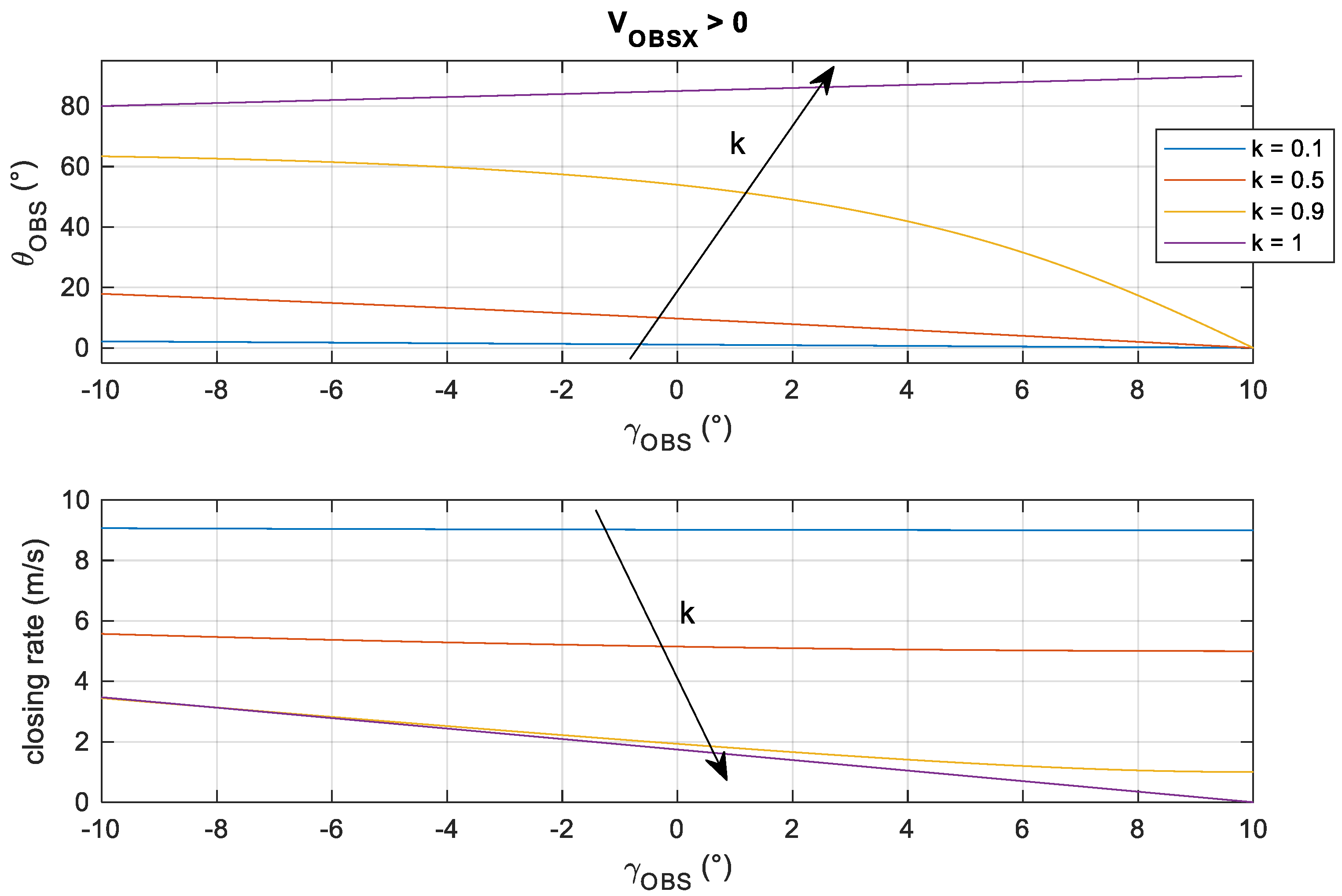
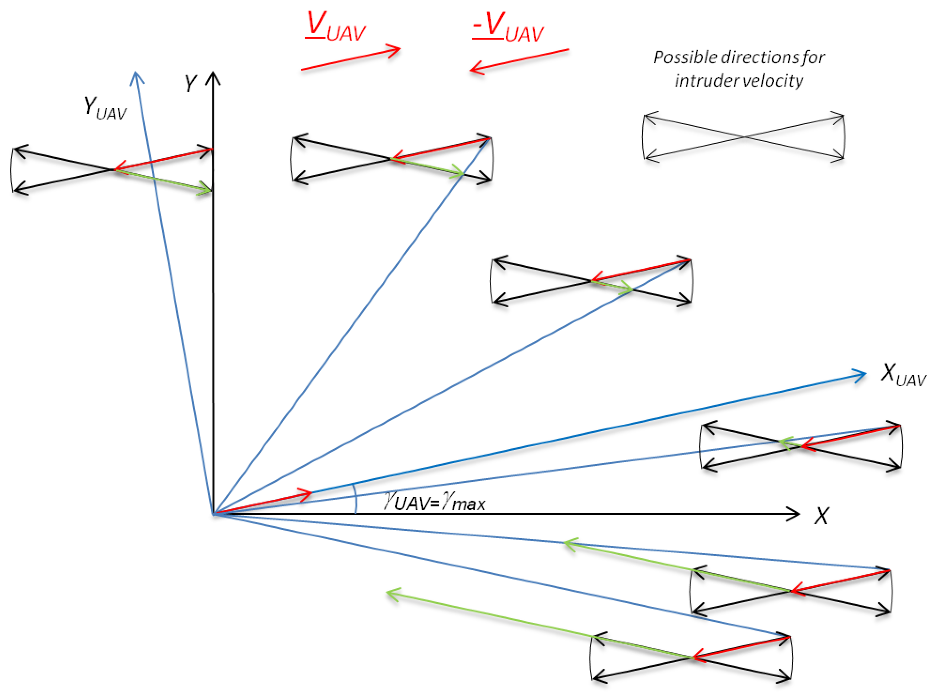
  • Fast encounters, i.e., corresponding to approaching geometries (VOBS,X < 0, so the UAV and the intruder move along opposite directions);
  • Slow encounters, i.e., corresponding to converging trajectories (VOBS,X > 0, so the UAV and intruder move along the same direction).
For given VUAV, k, γUAV, and γOBS, one or both of the encounters (or none of them) can be generated, depending on whether the negative range–rate condition (i.e., the second equation in (16)) is simultaneously satisfied. If this is the case, Equation (21) can be used to compute the maximum intruder elevation angles that can lead to collision conditions. For the sake of concreteness, let us consider the case γUAV = γmax = 10°. A dual analysis can be carried out for the descending flight. Then, let us assume VUAV = 10 m/s and γOBS ∈ [−10°, 10°]. Furthermore, let us consider multiple values for k, i.e., k = {0.1, 0.5, 0.9, 1, 1.1, 2}.
Figure 5 and Figure 6 show the values of θOBS, computed from (21), and of the resulting closing rate, computed as (VOBS,YUAV2 + (VOBS,XUAVVUAV)2)0.5, as a function of γOBS, for the different values of k. The fast and slow encounters are considered in separate diagrams. Clearly, the values of θOBS that correspond to the positive range rate, i.e., the condition in (16.b) is not met, are removed from the diagrams.
The analysis of (21), Figure 5 and Figure 6 lead to interesting conclusions.
  • If all the aircraft have the same flight path angle limits (i.e., γOBS is limited in the range [−10°,10°] in the diagrams), and the ownship is climbing with the maximum flight path angle, then fast encounters correspond to negative elevation angles, while slow encounters occur for positive elevation angles.
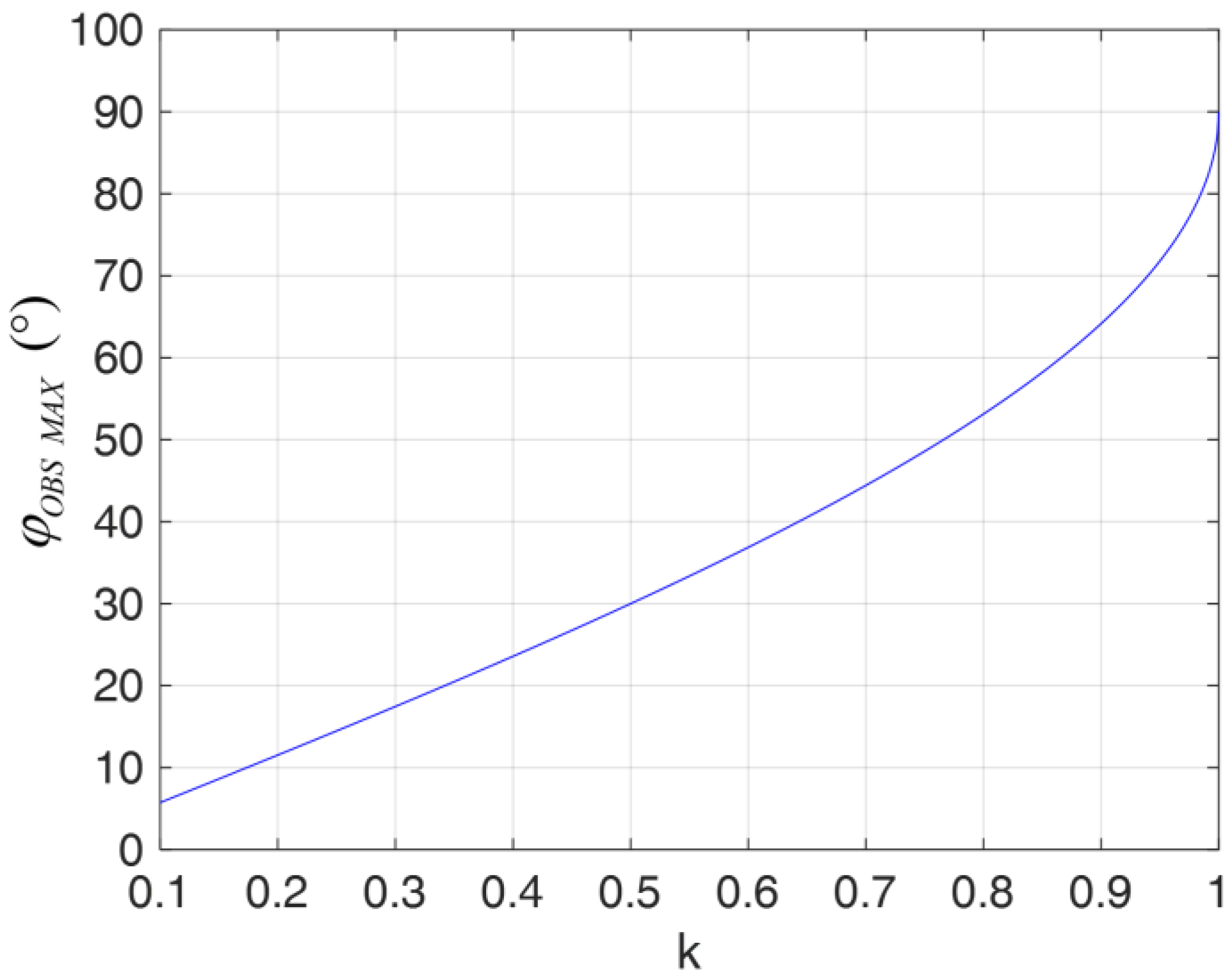
  • In the fast encounter case, the required FOV in elevation can be limited for any velocity ratio k by constraining the flight path angles. In fact, since θOBS functions are monotonic (see Figure 5), the largest negative obstacle elevation corresponds to the largest positive flight path angle for the obstacle. In particular, for |γOBSmax| = |γUAVmax| = γmax, the limit obstacle elevation angle (i.e., characterized by the maximum absolute value) can be obtained from (21) as follows.
tan θ O B S , a b s - m a x = k sin 2 γ m a x k cos 2 γ m a x + 1
  • Consequently, θOBS,abs-max tends to 0 for vanishing k (fixed obstacles), to γmax for k = 1, and to 2γmax if k approaches ∞.
  • Slow encounters (Figure 6) are generated only up to k ≃1 (i.e., for obstacles slower than the ownship). In these cases, θOBS,abs-max can be significantly larger than γmax. For k << 1, as in the fast encounter case, θOBS,abs-max vanishes (fixed obstacles). When k increases, the range of elevation angles in which collision geometries are generated increases, while the closing rate decreases. For equal velocities (k = 1), collision conditions can be generated at very large elevation angles (close to 90°), which correspond to quasi-parallel converging trajectories and thus very small closure rates. These conditions can be handled by selecting proper sensors with a relatively small detection range used only for surveilling the airspace above or below the aircraft. Moreover, extremely small range rate values could be considered of low impact in terms of collision risk. Constraining only flight path angles may not allow a reduction of the vertical FOV unless proper rules are also established for aircraft speeds (e.g., defining limited speed ranges can be useful to reduce closure rates that correspond to large elevation angles). These results have an immediate intuitive interpretation that derives from the flight path angle limits and the velocity ratio. A graphical representation to visualize some of the above-described collision conditions is provided in Figure 7.
In general, it is possible to relax sensing requirements on the elevation FOV based on dynamic constraints and/or flight rules that limit both flight path angles and speeds. In particular, the FOV that corresponds to a large closure rate (fast encounters) can be actually limited, while a trade-off between requirements on elevation angles and closure rates may be found for slow encounters. Equations (21) and (22) provide analytical tools to set these limits and optimize these trade-offs.

2.2. Effect of Non-Cooperative Sensing Performance on CPA Estimation Accuracy

It is intuitive that sensing accuracy, i.e., the error of the obstacle sensing system in estimating intruder relative position and velocity, impacts the performance of an SAA system in terms of the probability of missed and false conflict detections. In this framework, the critical parameters relevant to collision risk are the distance at CPA (dCPA), which actually has a vectorial nature, and its corresponding time (tCPA). To analytically derive the functional dependences between the CPA parameters and sensing uncertainties, following [1], let us consider a general 3D geometry as depicted in Figure 8, where A and B are the UAV and the obstacle, respectively, r is the relative position vector, and VAB is the relative velocity (i.e., the velocity of the UAV with respect to the obstacle).
Hence, assuming that both aircraft continue to fly with constant velocity, dCPA is given by
d ¯ C P A = r ¯ V ¯ A B V ¯ A B 2 V ¯ A B r ¯
while tCPA is computed as shown below.
t C P A = r ¯ V ¯ A B V ¯ A B 2
Though tracking algorithms may work on Cartesian coordinates, non-cooperative sensing systems typically produce obstacle information expressed in terms of range, range rate, and/or angles. Hence, it is useful to express the relative position and velocity vectors in terms of spherical coordinates, i.e., range (r), azimuth (φ), and elevation (θ), and their first order derivatives ( r ˙ , φ ˙ , θ ˙ ), within a North-East-Down (NED) reference frame with the origin at the UAV position, thus obtaining the following relations.
r ¯ = r cos φ cos θ r sin φ cos θ r sin θ
V ¯ A B = d r ¯ d t = r ˙ cos φ cos θ + r φ ˙ sin φ cos θ + r θ ˙ cos φ sin θ r ˙ sin φ cos θ r φ ˙ cos φ cos θ + r θ ˙ sin φ sin θ r ˙ sin θ + r θ ˙ cos θ
By substituting (25) and (26) into (23), dCPA can be written as follows
d ¯ C P A = d C P A , n d C P A , e d C P A , d = r r ˙ r ˙ 2 + r 2 θ ˙ 2 + φ ˙ 2 cos 2 θ r ˙ cos φ cos θ + r φ ˙ sin φ cos θ + r θ ˙ cos φ sin θ r ˙ sin φ cos θ r φ ˙ cos φ cos θ + r θ ˙ sin φ sin θ r ˙ sin θ + r θ ˙ cos θ r cos φ cos θ r sin φ cos θ r sin θ
where dCPA,n, dCPA,e, and dCPA,d are the cartesian components of dCPA in NED. It is now useful to distinguish the horizontal and the vertical components of dCPA. They are defined hereunder,
d C P A , h o r = d C P A , n 2 + d C P A , e 2 d C P A , v e r = d C P A , d
and can be expressed in terms of range, azimuth, elevation, and their first derivative by combining (27) and (28).
d C P A , h o r = r 2 r cos θ θ ˙ 2 + φ ˙ 2 cos 2 θ + r ˙ θ ˙ sin θ 2 + r ˙ 2 φ ˙ 2 cos 2 θ r ˙ 2 + r 2 θ ˙ 2 + φ ˙ 2 cos 2 θ
d C P A , v e r = r 2 r ˙ θ ˙ cos θ + r sin θ θ ˙ 2 + φ ˙ 2 cos 2 θ r ˙ 2 + r 2 θ ˙ 2 + φ ˙ 2 cos 2 θ
Under the assumption of small and uncorrelated errors, the uncertainty (σ) in the estimated components of dCPA can be calculated by a first-order propagation of sensing uncertainties on range, angles, and their derivatives ( r , φ , θ , r ˙ , φ ˙ , θ ˙ ), as follows.
σ d C P A , h o r 2 = d C P A , h o r r 2 σ r 2 + d C P A , h o r φ 2 σ φ 2 + d C P A , h o r θ 2 σ θ 2 + d C P A , h o r r ˙ 2 σ r ˙ 2 + d C P A , h o r φ ˙ 2 σ φ ˙ 2 + d C P A , h o r θ ˙ 2 σ θ ˙ 2
σ d C P A , v e r 2 = d C P A , v e r r 2 σ r 2 + d C P A , v e r φ 2 σ φ 2 + d C P A , v e r θ 2 σ θ 2 + d C P A , v e r r ˙ 2 σ r ˙ 2 + d C P A , v e r φ ˙ 2 σ φ ˙ 2 + d C P A , v e r θ ˙ 2 σ θ ˙ 2
In this respect, it is critical to point out that the obstacle state parameters are assumed to be determined from sensor measurements but after the transition to firm tracking. This means that the uncertainties in (31) and (32) are independent of the specific non-cooperative sensor adopted (e.g., radar, LIDAR, or cameras). Thus, the general applicability of this approach arises. Hence, the impact of tracking accuracies on the uncertainty of the dCPA can be determined by computing (without approximations) the first-order derivatives in (31) and (32) and adopting a numerical approach (which can be undertaken in real-time too).
Clearly, (29) and (30) show that no direct relation between dCPA and the azimuth angle φ exists. Hence, the azimuth accuracy (σφ) has no impact on the relative motion problem. However, the azimuth angle plays an indirect role as it affects the ttc for the assigned relative range (as highlighted in the previous subsection).
Aiming to define sensing requirements and to link them with the other problem variables, an analytical approach is here followed. The main idea is to find approximated expressions for the above derivatives based on an analysis of the orders of magnitude of the different terms composing each equation in near-collision encounters. When applicable, the assumption of low elevation can be used to provide further simplifications. Specifically, in general, two equivalent approaches can be exploited.
  • The analysis of the order of magnitude (based on the conditions of a near-collision encounter) is applied to the exact expressions of the derivatives of dCPA,hor and dCPA,ver.
  • First, approximated expressions for dCPA,hor and dCPA,ver are obtained under the assumption of near-collision encounters. Second, the corresponding derivatives are computed. Finally, the different contributions are compared based on their order of magnitude.
Although, approach A is more rigorous, at first order they produce the same results, and approach B is adopted here for mathematical simplicity. First, the mathematical relation defining a near-collision encounter can be written as follows
O r φ ˙ r ˙ = O r θ ˙ r ˙ = ε , ε < < 1 ,
where O(-) is the order of magnitude operator. Under these conditions, the following relation also holds.
t C P A r r ˙ ,
Please note that the equivalence in (34) applies since, for scenarios of interest, the range rate is negative. Within the collision avoidance scenarios of interest, tCPA is bounded, being, at most, of the order of a few tens of seconds, as stated in (35).
O φ ˙ = O θ ˙ = ε t C P A ,
Hence, the order of magnitude of the terms appearing within (29) and (30) can be evaluated.
O r cos θ θ ˙ 2 + φ ˙ 2 cos 2 θ = O r sin θ θ ˙ 2 + φ ˙ 2 cos 2 θ = ε 2 t C P A r ˙ ,
O r ˙ θ ˙ sin θ = O r ˙ θ ˙ cos θ = ε t C P A r ˙ ,
O r 2 θ ˙ 2 + φ ˙ 2 cos 2 θ = r ˙ 2 ε 2 ,
The analysis of the order of magnitude given by (36)–(38) leads to the following relations.
r cos θ θ ˙ 2 + φ ˙ 2 cos 2 θ < < r ˙ θ ˙ sin θ ,
r ˙ 2 θ ˙ 2 + φ ˙ 2 cos 2 θ < < r ˙ 2 ,
r s i n θ θ ˙ 2 + φ ˙ 2 cos 2 θ < < r ˙ θ ˙ cos θ ,
If (39) and (40) are considered within (29), while (40) and (41) are considered within (30), dCPA,hor and dCPA,ver can be approximated as follows.
d C P A , h o r r 2 r ˙ θ ˙ 2 sin θ 2 + φ ˙ 2 cos θ 2 = r 2 r ˙ θ ˙ 2 sin θ 2 + φ ˙ 2 cos θ 2 ,
d C P A , v e r r 2 r ˙ θ ˙ cos θ ,
Hence, the derivatives of dCPA,hor and dCPA,ver with respect to the UAV-intruder relative state parameters in spherical coordinates (i.e., r , φ , θ , r ˙ , φ ˙ , θ ˙ ) can be computed. They are collected in Table 1, which also reports their order of magnitude, computed consistently with the above assumptions.
As a result of this analysis, it can be stated that, in the case of near-collision encounters, the uncertainty in dCPA,hor mainly depends on σ φ ˙ and σ θ ˙ , while the uncertainty in dCPA,ver mainly depends only on σ θ ˙ . Indeed, all the remaining derivates are smaller or 0. The final expressions for the non-negligible derivatives are provided below.
d C P A , h o r φ ˙ r 2 cos 2 θ r ˙ ,
d C P A , h o r θ ˙ r 2 sin 2 θ r ˙ ,
d C P A , v e r θ ˙ r 2 cos θ r ˙ ,
The consistency between (44)–(46) and the exact derivatives of dCPA,hor and dCPA,ver, evaluated in near-collision conditions, has been verified numerically (see Section 3.1). Focusing on dCPA,hor, it is interesting to analyze the relative importance of the two contributions as a function of the elevation angle. Clearly, in low elevation conditions (i.e., θ << 1), sin(θ) ≈ θ (thus being an infinitesimal quantity), while cos(θ) ≈ 1. So, the uncertainty in the estimation of the elevation rate at firm tracking does not have a significant effect on dCPA,hor. More generally, in near-collision and low-elevation conditions, the coupling between horizontal and vertical quantities and the sensitivity to the elevation angle itself become negligible.
Within Table 1, orders of magnitude have been expressed by using tCPA as the fundamental dimensional parameter. This choice is related to the fact that tCPA is the basic variable defining the available time for collision avoidance maneuvering. The range rate also appears in some derivatives, and it can be computed with simplified models, as will be further discussed in Section 2.3.
The adopted analytical approach and the derivatives presented in Table 1 provide direct insight into the impact of sensing parameters on the accuracy of the estimation of the CPA, thus supporting sensor design and/or selection. As an example, given a sensor that is able to provide range measurements, it is likely that the design trade-off should be aimed at increasing the detection range at the expense of range and range rate resolution, given their limited importance for the estimation of collision conditions. In the practical case of a pulsed radar, this means selecting relatively long pulses.
As mentioned earlier in this section, since the uncertainties in (31) and (32) conceptually correspond to tracker outputs (despite the primary source of uncertainty being the sensor itself), other effects must be accounted for.
  • As tracking algorithms usually work in stabilized coordinates and account for ownship motion, navigation unit performance may impact tracking uncertainty. This may be especially true for small UAS which can equip very high angular resolution sensors (e.g., LiDAR) and relatively low-performance inertial units. Also, sensors are assumed to be aligned with velocity. In the case of strapdown installation and non-negligible attitude angles, the final uncertainty on stabilized coordinates may merge sensor uncertainties in azimuth and elevation.
  • Tracking uncertainty also includes the measurement rate and the probability of detection, which together impact the effective valid measurement rate when firm tracking is achieved.
Different angular uncertainties in azimuth and elevation lead to different uncertainties in horizontal and vertical dCPA. This difference may impact the selection of the avoidance maneuvers, but in general, the uncertainty in a given direction has to be traded off against vehicle maneuverability. Of course, if vehicle maneuverability or flight rules bias the maneuver towards a given direction, then the angular uncertainty in the other direction may play a more limited role. This is true if we focus on horizontal collision avoidance. However, cross-correlation effects are produced if the elevation is not negligible. In this case, the analytical expressions directly allow the estimation of this cross-correlation effect, so they can be used as guidance for relaxing sensing requirements in elevation.
Finally, it is important to underline that the azimuth angle apparently plays no role in impacting the CPA accuracy. This is a direct consequence of having formulated the problem in relative terms. Indeed, the azimuth angle is fundamental in determining the link between aircraft velocities, range, and range rates for given tCPA. Its impact is discussed in the next subsection.

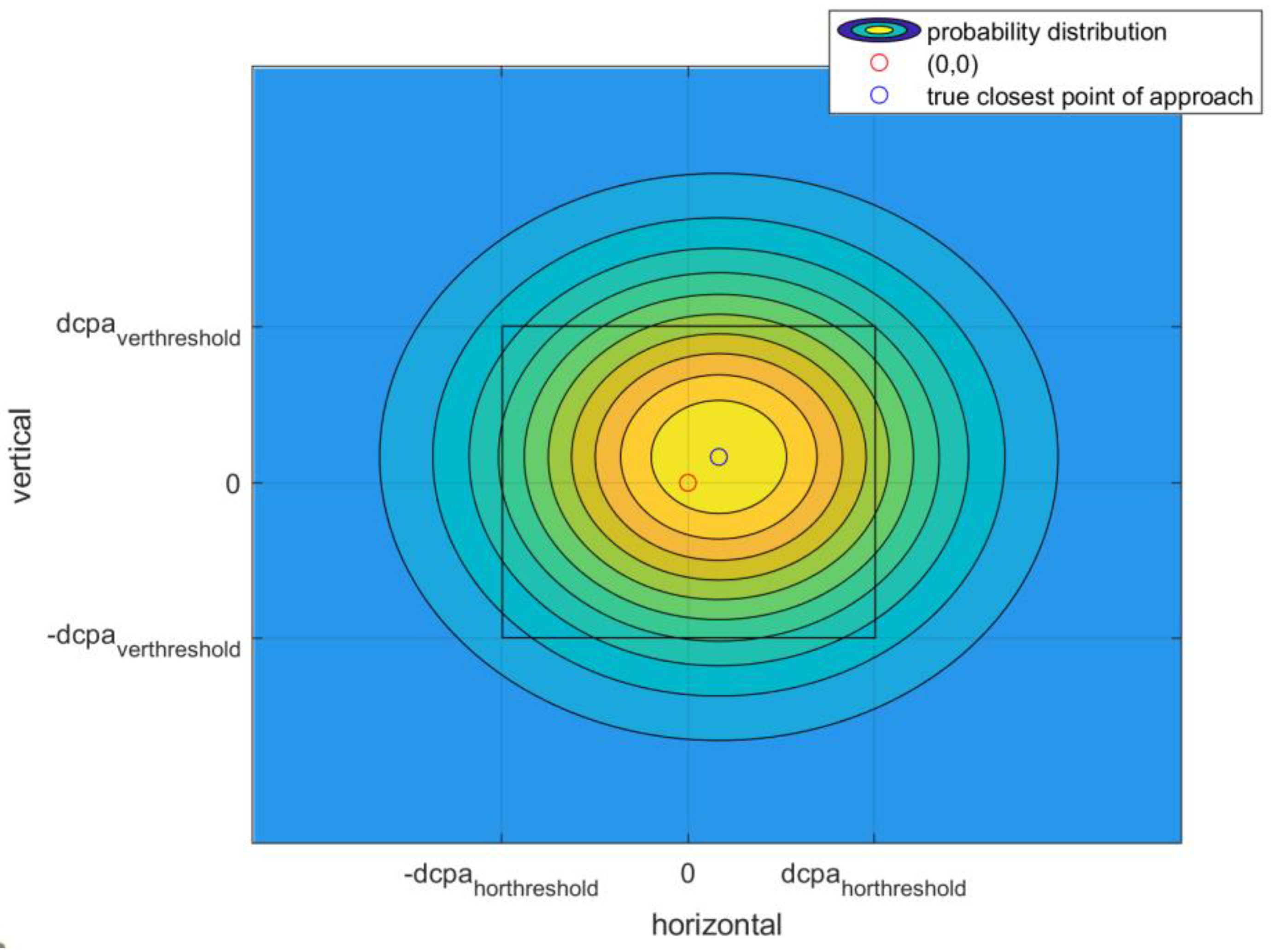
2.3. Integrated Range-Accuracy Requirements

The previous derivations on FOV effects and accuracy can be exploited, together with the other sensing performance parameters (e.g., detection range, measurement rate, and integrity, i.e., the confidence on tracking outputs), to derive integrated requirements for non-cooperative SAA. As noted in [7] and [19], from a conflict detection perspective, an SAA sensing system can be characterized by two probabilities, namely, the probability of missed conflict detection and the probability of false conflict detection.
In this framework, the probability of missed detection is defined as the probability that the system will not provide any collision alert, given that a conflict is present. Conversely, the probability of false conflict detection is the probability of providing a collision alert when no collision threats are present. Actually, this represents the basic parameter measuring situational awareness and combines detection range performance, the probability of generating false tracks, tracking accuracy, and adopted conflict detection criteria, while also depending on relative motion geometry. The previous literature has focused on the link between probabilities and tracking accuracy [7]. This paper generalizes these findings addressing concepts that were preliminary discussed in [19].
Detection for non-cooperative sensors is a stochastic phenomenon that can be modeled by defining a probability of detection, which is a function of range. In general, for a given sensor, this will depend on the tuning choices for the intruder detection process. From the SAA system perspective, a parameter that is more important than detection range is the declaration range, representing the range where the information about the existence of an intruder is considered reliable enough to be transmitted to subsequent processing steps such as conflict detection and collision avoidance. This usually happens when the tracking algorithm switches to firm tracking, which means that a minimum number of associated measurements have been acquired. In theoretical terms, the range at which firm tracking is achieved depends on the probability of detection, measurement rate, and range rate of the intruder, which introduces a dependency on the position of the intruder in the FOV. However, at the first level of approximation, the dependency on range rate can be neglected and it is possible to define a probability of firm tracking (PFT) which only depends on range.
In general, a missed conflict detection for an existing intruder can be due to two phenomena.
  • The intruder has not been declared yet. The corresponding probability is given by 1 − PFT.
  • The intruder has been declared and its relative dynamics lead to a conflict, but tracking error and decision-making criteria do not lead to positive conflict detection. The corresponding probability is the result of the product between PFT and an additional term depending on the tracking accuracy (PMD,track_acc).
In general, the estimation of PMD,track_acc requires the definition of a conflict detection criterion. Consistent criteria can be defined if errors on dCPA and tCPA are assumed to be normally distributed, as undertaken in [8], which then focuses on uncertainties in tCPA and dCPA,hor. When dealing with non-cooperative SAA, intruder declaration is usually carried out at a relatively low ttc. Based on this consideration, in this work, as in [1], it is assumed that a conflict is declared based on spatial variables only (dCPA,hor and dCPA,ver), e.g., considering thresholds that include sensing uncertainties. Thus, the probability of missed conflict detection for an existing intruder PMD,track_acc can be evaluated as a two-dimensional integral computed outside an area defined by the assumed limits on the dCPA,hor and dCPA,ver. The concept is shown in Figure 9. The two-dimensional probability distribution is conceptually centered on the true value (blue circle), thus the probability depends on the latter.
So, the total probability of missed conflict detection (PMD) can be evaluated using (47).
P M D = 1 P F T + P F T P M D , t r a c k , a c c ,
A similar discussion can be carried out for the probability of false conflict detection. Considering again the case of a single intruder, it is, in general, the sum of two contributions.
  • A false intruder is declared, and its estimated kinematics generate a positive conflict detection. The overall probability is given by the product of the probability of false track generation (Pfalse_track) times the probability that this false track corresponds to a conflict (Pfalse_track_conflict). Pfalse_track depends on the settings adopted for the detection and the tracking algorithm, and on the operating environment. Pfalse_track_conflict is a parameter that can be assumed as a constant and mainly depends on the adopted conflict detection criteria.
  • The intruder has been declared and its relative dynamics dooes not lead to a conflict, but tracking errors and decision-making criteria lead to positive conflict detection. The corresponding probability is the result of the product between PFT and an additional term depending on the tracking accuracy (PFA,track_acc). Again, this latter term can be estimated as a two-dimensional integral based on the components of the dCPA.
So, the two probabilities can be combined as shown in (48).
P F A = min 1 , P f a l s e _ t r a c k P f a l s e _ t r a c k _ c o n f l i c t + P F T P F A , t r a c k , a c c ,
The trends of these general parameters can be analyzed by combining the previous discussions about FOV effects and sensing uncertainties, based on the approximated dCPA equations. Let us focus for simplicity on a low-elevation case and thus only on dCPA,hor. Under this assumption, (42) can be written as follows,
d C P A , h o r t C P A 2 r ˙ φ ˙ ,
where r ˙ is a function of VUAV, VOBS, and φ. Let us now assume a fixed tCPA, based on the idea outlined above. The dependency of range rate from the azimuth angle can be found analytically by a construction that is similar to the one in Figure 1. Let us consider again a 2D (horizontal) approximation as in Figure 10.
Applying the Carnot theorem to the triangle of velocities, (50) holds,
V O B S 2 = V O B S U A V 2 + V U A V 2 2 V O B S U A V V U A V cos φ γ = 0 ,
where
γ = arcsin d C P A R ,
Thus, the relative velocity and the closure rate can be obtained using (52) and (53), respectively.
V O B S U A V = V U A V cos φ γ + V O B S 2 V U A V 2 sin 2 φ γ ,
r ˙ = V O B S U A V cos γ = V U A V cos φ γ + V O B S 2 V U A V 2 sin 2 φ γ cos γ ,
It is worth noting that the sign ‘+’ before the square root either corresponds to the unique solution (with negative range rate) or to the fastest encounter when the ‘−’ sign is also a physically meaningful conflict (the latter case happens for intruders that are slower than the ownship within a limited field of view around the velocity direction, as noted in Section 2.1). In near-collision conditions, d C P A r r φ ˙ r ˙ 1 and γ 1 , so (54) holds.
r ˙ V U A V cos φ + V O B S 2 V U A V 2 sin 2 φ
This equation expresses the dependence of range rate on intruder azimuth in near-collision conditions for given ownship and intruder velocities. While its information content is similar to (10), relevant to the variation of the tCPA as a function of azimuth, it provides a direct expression for the effect of conflict geometry on the propagation of sensing uncertainty. In fact, recalling (49) (i.e., the approximated equation for dCPA,hor) and focusing only on azimuth rate uncertainty as the error source, the following relation can be written.
σ d C P A , h o r t C P A 2 r ˙ σ φ t C P A 2 V U A V cos φ + V O B S 2 V U A V 2 sin 2 φ σ φ
This equation clearly shows that, for constant tCPA and given sensing uncertainty, the final uncertainty on the CPA reduces moving towards lateral areas of the FOV. As a consequence, a sensing system with the same performance levels in the whole FOV will, in general, provide varying conflict detection performance depending on the variation of the range rate to the conflicting obstacles. If it is designed on the basis of worst-case frontal collision scenarios, it will tend to be overconservative for lateral conflicts. On the other hand, it is possible to keep the same safety level in the whole FOV by installing a sensing system with variable features, i.e., by relaxing sensing accuracy as lateral areas of the FOV are dealt with.
More generally, it is possible to have a sensing system with a variable detection range, measurement rate, and/or accuracy in the FOV around the ownship velocity vectors, keeping the same levels of safety. The key point is to account for the closure rates of near-collision intruders, which involve the ownship speed and the expected non-cooperative traffic. Also, sensing characteristics can be adapted in real time depending on UAV velocity, which allows for better exploitation of sensing resources.
The derived analytical relations provide a tool for quantitative assessment of how different requirements can be combined with each other, and how they interact with the characteristics of the airspace and the current UAV velocity. Indeed, these relations are also useful in the case of visual systems, where, although 3D relative state estimation may be unfeasible, it is still possible to consider conflict detection criteria that involve worst case assumptions on range and range rate [9].

3. Numerical Analyses

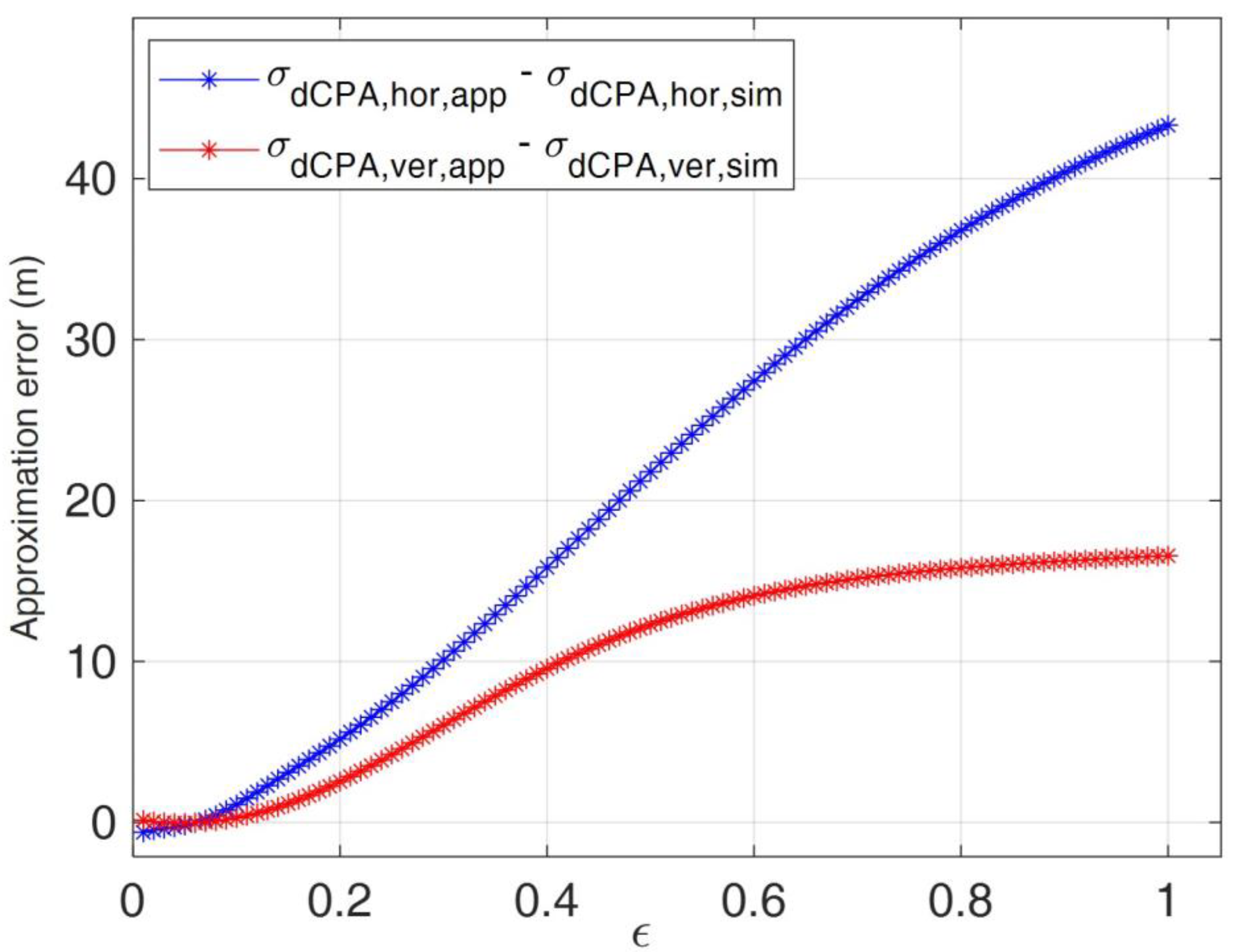
3.1. Statistical Consistency

The goal of this subsection is to demonstrate the statistical consistency of the approximated expressions obtained in Section 2.2 for the derivatives of dCPA,hor and dCPA,ver with respect to the obstacle state parameters. Indeed, these derivatives can be used to accurately estimate the dCPA uncertainty under near-collision conditions for given firm tracking uncertainties, thus being extremely useful when designing a sensor architecture for non-cooperative SAA. Let us consider the relative motion scenario identified by the parameters in Table 2.
The near-collision condition indicated by (33) is satisfied since ε=O( r φ ˙ r ˙ ) is 10−3. In fact, the exact values of dCPA,hor and dCPA,ver, computed using (29) and (30), are equal to 6.90 m and 3.45 m, respectively. Moreover, the tCPA (≈20 s) is consistent with the time required by an avoidance maneuver [1]. At this point, a set of 1,000,000 random simulations is run adding a Gaussian white noise (whose standard deviations are given by the uncertainties reported in Table 2) to the true obstacle state parameters to reproduce the output of the tracking filter. For each simulation, dCPA,hor and dCPA,ver can again be computed using (29) and (30), thus obtaining the statistical distribution depicted by the histograms in Figure 11. It is interesting to note that although by definition dCPA,hor should always be positive, its real sign has been assigned based on the collision direction (which is given by the sign of dCPA,y).
At this point, the horizontal and vertical dCPA uncertainties can be computed from the above statistical distributions (i.e., σdCPA,hor,sim and σdCPA,ver,sim), as well as by substituting into (31) and (32) the approximated, non-negligible derivatives given by (44)–(46), thus obtaining σdCPA,hor,app and σdCPA,ver,app. The results collected in Table 3 show that the order of magnitude analysis carried out in Section 2.2 can be exploited to accurately estimate the dCPA uncertainties if the near-collision conditions are satisfied.
It is now interesting to show how accurate this approximation becomes as the obstacle state parameters move away from the near-collision conditions. This can be performed at a fixed tCPA, increasing the azimuth and elevation rates. Figure 12 shows the increase in the approximation error as ε goes from 10−2 to 1.

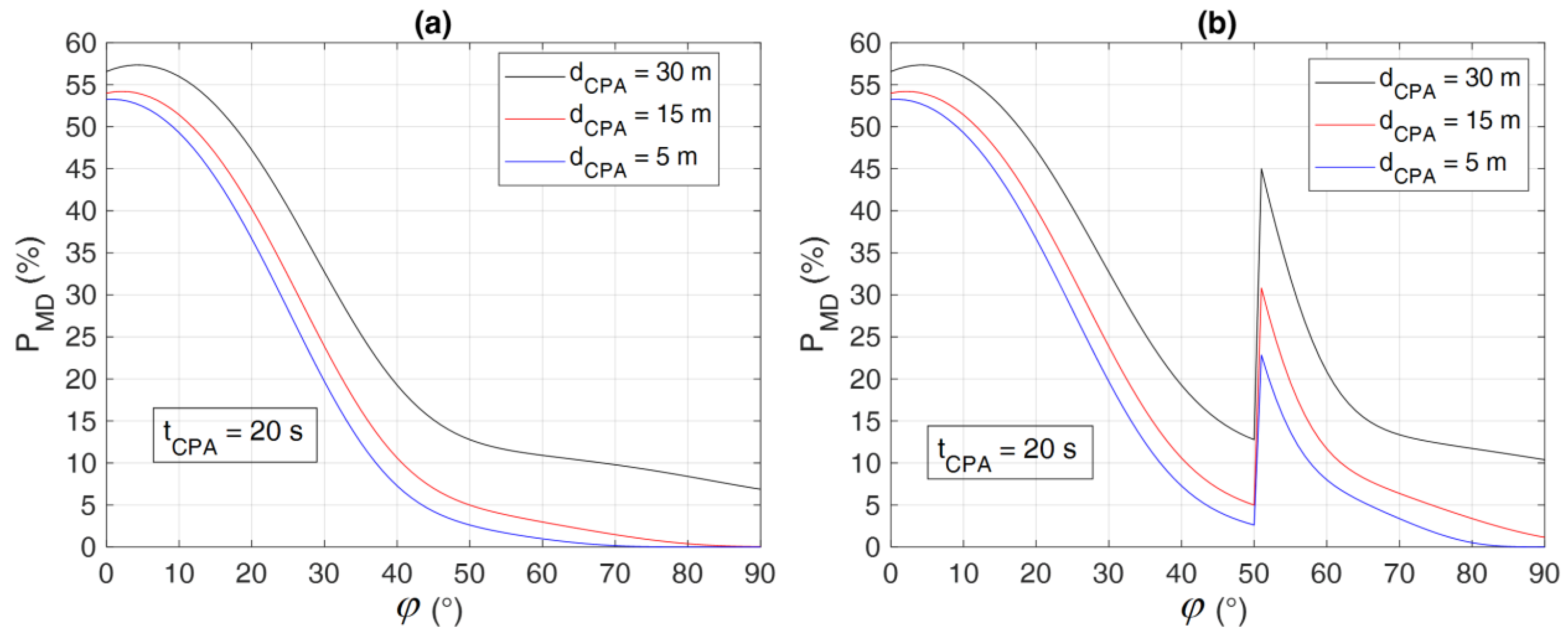
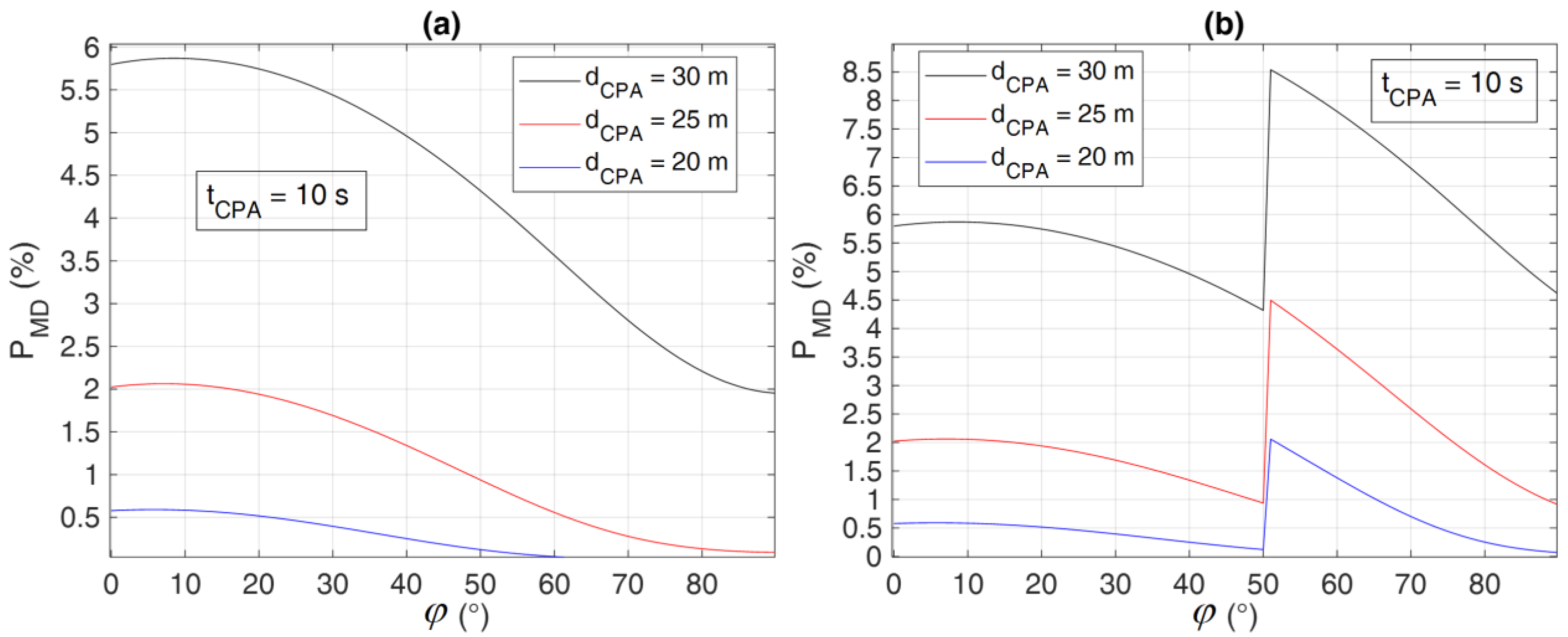
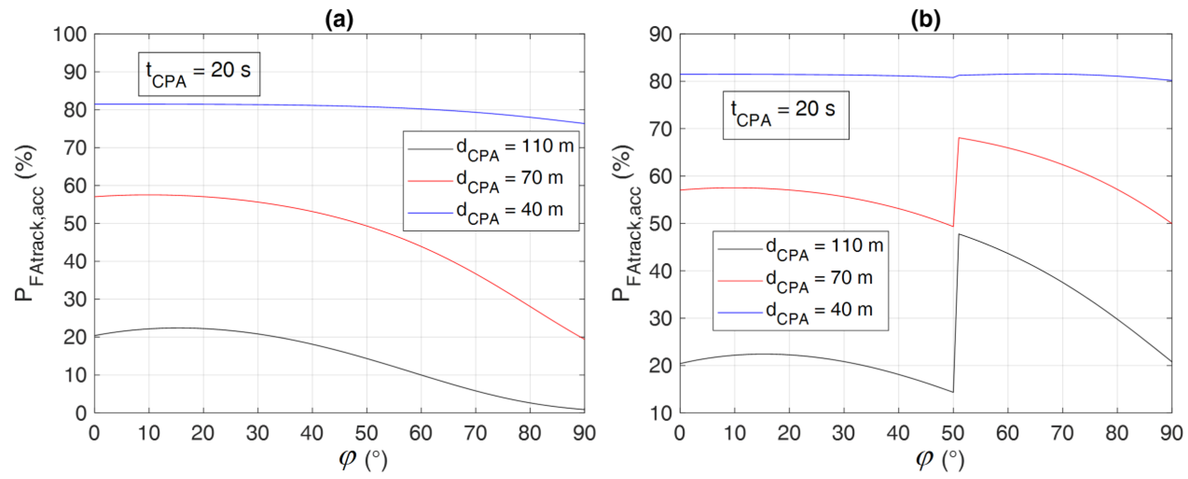
3.2. Evaluation of Conflict Detection Performance

The goal of this subsection is twofold. First, it aims to quantitatively demonstrate how conflict detection performance levels, i.e., PMD and PFA, which are evaluated according to the discussion in Section 2.3, vary depending on the obstacle position in the FOV to be monitored. Indeed, this occurs independently of the specific technological solution adopted for a non-cooperative SAA architecture, i.e., based on active (e.g., RADAR-based), passive (e.g., camera-based), or hybrid (e.g., RADAR-camera-based) sensors. The second goal is to show how this phenomenon can be exploited to relax sensor requirements, i.e., to ensure adequate levels of safety in the entire FOV, while simultaneously optimizing onboard resources in terms of sensors’ weight and cost.
For the sake of mathematical simplicity, the following analysis is carried out simulating 2D (horizontal) collision scenarios. An example of a 2D collision geometry is depicted in Figure 13, where frontal and lateral areas of the FOV to be monitored are highlighted with different colors to account for the possibility of using different sensors to cover them (taking the typical FOVs of existing sensors into account).
The simulated scenario is defined assigning VUAV and VOBS, as well as the tracking uncertainties in the obstacle state parameters, i.e., range ( σ r ), range rate ( σ r ˙ ), and azimuth rate ( σ φ ˙ ), which represent a measure of the accuracy level of the firm track generated by the SAA system. Clearly, the tracking uncertainties depend not only on the onboard sensors in charge of the SAA function, but also on the implemented tracking algorithm. So, the following probabilities, i.e., PFT, Pfalse_track, and Pfalse_track_conflict, must be determined to complete the characterization of firm tracking performance for the SAA system under analysis. As already anticipated in Section 2.3, PFT depends on the declaration range (rft), i.e., the range at which a firm track is created, which can be modeled as a Gaussian random variable with the mean (μr,ft) and standard deviation (σr,ft) to be selected based on the specific sensor architecture. Hence, if track-loss phenomena are neglected, PFT can be computed as follows,
P F T = 1 c d f ( r f t ) ,
where cdf is the cumulative distribution function. Instead, the estimation of Pfalse_track and Pfalse_track_conflict is complex, since their values depend on the setting of the tracking algorithm as well as on the adopted conflict detection criterion. So, a conservative solution can be undertaken by assuming that their product is equal to 0.01, which implies that the firm tracking process causes an increase in PFA of 1%. Given all the inputs, the simulator is designed to compute PMD and PFA as a function of three variables, i.e., tCPA, dCPA, and φ. To obtain meaningful conflict scenarios, the simulator is run varying the following parameters:
  • tCPA is varied between 0 s and 50 s;
  • dCPA is varied between 0 m and 120 m;
  • φ is varied between −90° and 90°.
It is worth noting that the analysis of results will be limited to positive values of φ. This is justified by the fact that conflict detection performance will have symmetric behavior in the FOV provided that the installation of the selected non-cooperative sensors is appropriate. Once the interval of interest for these independent variables is defined, the intruder range corresponding to each triple (dCPA, φ, tCPA) must be determined. If (51) and (52) are substituted within (24), the relation shown in (57) can be obtained for tCPA.
t C P A = r cos arcsin d C P A r V U A V cos φ arcsin d C P A r + V O B S 2 V U A V 2 sin φ arcsin d C P A r ,
The equation above is implicit with respect to the unknown value of r. Thus, it can be solved numerically.
At this point, the simulations are performed considering two radar-based architectures for non-cooperative SAA. Both VUAV and VOBS are set to 10 m/s. The threshold on dCPA that defines the existence of a conflict (i.e., the assumed separation minimum) is set to 36 m, consistent with dense, low-altitude airspace scenarios. As explained in [22], the assumed conflict detection criteria add to this minimum separation a safety margin equal to the estimated σdcpa. In the first architecture (SAARADAR-1), the same “high-level” radar is selected to cover the entire horizontal FOV(i.e., both the frontal and lateral areas with reference to Figure 13), while in the second architecture (SAARADAR-2), a “low- level” radar is selected to look for non-frontal obstacles (i.e., to cover the lateral FOV in Figure 13). Specifically, it is assumed that the “low-level” radar has worse performance in terms of azimuth rate accuracy, and declaration range. Hence, the parameters characterizing SAARADAR-1 and SAARADAR-2 are collected in Table 4.
Consistent with the discussions included in Section 2, fixed values of tCPA (which is a direct measure of the time available to perform the avoidance maneuver) are selected, so that the estimated PMD and PFA can be depicted as a function of φ and dCPA. For instance, if tCPA is set to 20 s, the resulting PMD is depicted in Figure 14 for the two radar-based architectures.
Figure 14a quantitatively shows how the conflict detection performance of SAARADAR-1 improves as φ increases. Although this phenomenon occurs for any value of dCPA, it gets more and more evident for decreasing dCPA. Indeed, if, for instance, dCPA is 30 m, PMD varies from 56.8% along boresight to a residual 8.1% at φ = 90°. On the other hand, if dCPA is 5 m, PMD varies from 53.3% along boresight to 10−10% at φ = 90°. Figure 14b is obtained considering SAARADAR-2. The transition between the two portions of the horizontal FOV covered by the high- and low-performance radars, which occurs at φ = 50°, is identified by a discontinuity (namely, a sudden increase) in the variation of PMD as a function of φ for any value of dCPA. However, it is interesting to show that the value of PMD for φ > 50° is still smaller than its maximum value obtained along boresight. This example shows how it is possible to save onboard resources (e.g., in terms of weight and power consumption) by selecting lower-level SAA sensors without compromising conflict detection performance.
The same comparison can be undertaken also for tCPA = 10 s, which corresponds to a more critical scenario for the realization of the collision avoidance maneuver. The resulting PMD is depicted in Figure 15 for the two radar-based architectures.
In this case, the maximum value of PMD is around 16% (at dCPA = 36 m) and its reduction with φ is still present, though less evident for both SAARADAR-1 and SAARADAR-2. Indeed, due to the lower range of the intruder, PFT is practically 100% in the entire φ-dCPA plane, so collision detection performance is regulated mainly by the sensing accuracy. Although in this case for SAARADAR-2, the lateral PMD (φ > 50°) becomes slightly larger than its maximum value provided by the better sensor in frontal conditions, the leap characterizing the discontinuity in the PMD variation at φ = 50° (see Figure 15b) is actually very small. In fact, the maximum PMD leap as a function of dCPA is around 4.3% when dCPA is 28 m, while if tCPA is 20 s, the PMD leap varies from 17.4% when dCPA is 0 m to 33% when dCPA is 36 m. Finally, it is worth highlighting that PMD is lower than 1% for any φ if dCPA is less than 22 m and 16 m for SAARADAR-1 and SAARADAR-2, respectively.
With regards to the PFA, the performance achieved by the two analyzed SAA architectures is shown in Figure 16, again considering a tCPA equal to 20 s. Two important aspects must be highlighted. First, the PFA is subject to significant variation as a function of the intruder position in the horizontal FOV. However, this PFA behavior is not characterized by a monotonic reduction with φ, as it occurs for the PMD. Second, in the SAARADAR-2 architecture, the transition to the lateral sensor at φ = 50° generates a sudden reduction in the false alarm probability. Both these apparently strange phenomena are due to the interaction between the two contributors to the final PFA value, i.e., sensing/tracking accuracy and the probability of firm tracking. The non-monotonic behavior of the overall PFA can be explained considering that for increasing azimuth angles the probability of firm tracking increases, thus indirectly generating an increase in the PFA, while the contribution of sensing accuracy PFAtrack,acc decreases due to the range rate reduction shown in Equation (55). Indeed, if only the sensing accuracy contribution is considered, the resulting PFA (PFAtrack,acc) is depicted in Figure 17 for the two radar-based architectures. As expected, both the plots show a monotonic reduction of PFAtrack,acc at increasing azimuth, while the PFA discontinuity at φ = 50° for SAARADAR-2 is a sudden increase in that probability.
When tCPA is 20 s, the overall PFA value is quite high (e.g., larger than 20%) over a large portion of the φ-dCPA plane. However, it is interesting to highlight its significant reduction if a smaller value of tCPA is considered. The overall PFA for the two architectures considering a tCPA of 10 s is shown in Figure 18. For this scenario, the PFA is lower than 10% for any φ if dCPA is larger than 62 m and 81 m for SAARADAR-1 and SAARADAR-2, respectively. Moreover, in this case, the transition to the lateral sensor implies an increase in the maximum PFA value.

4. Conclusions

This paper addressed sensing requirements for non-cooperative sense and avoid adopting an integrated and analytical approach to extract main dependencies and sensitivities. Based on approximations that are valid in near-collision conditions, analytical relations were derived which describe the variation of conflict conditions within the vehicle field of regard, both in azimuth and in elevation, the effects of sensing accuracy, and their interaction with the stochastic nature of obstacle detection and tracking. The derived relations were validated through numerical examples, which are also useful to point out the variation of sensing performance as a function of the encounter geometry and speeds. The main results can be summarized through the following points.
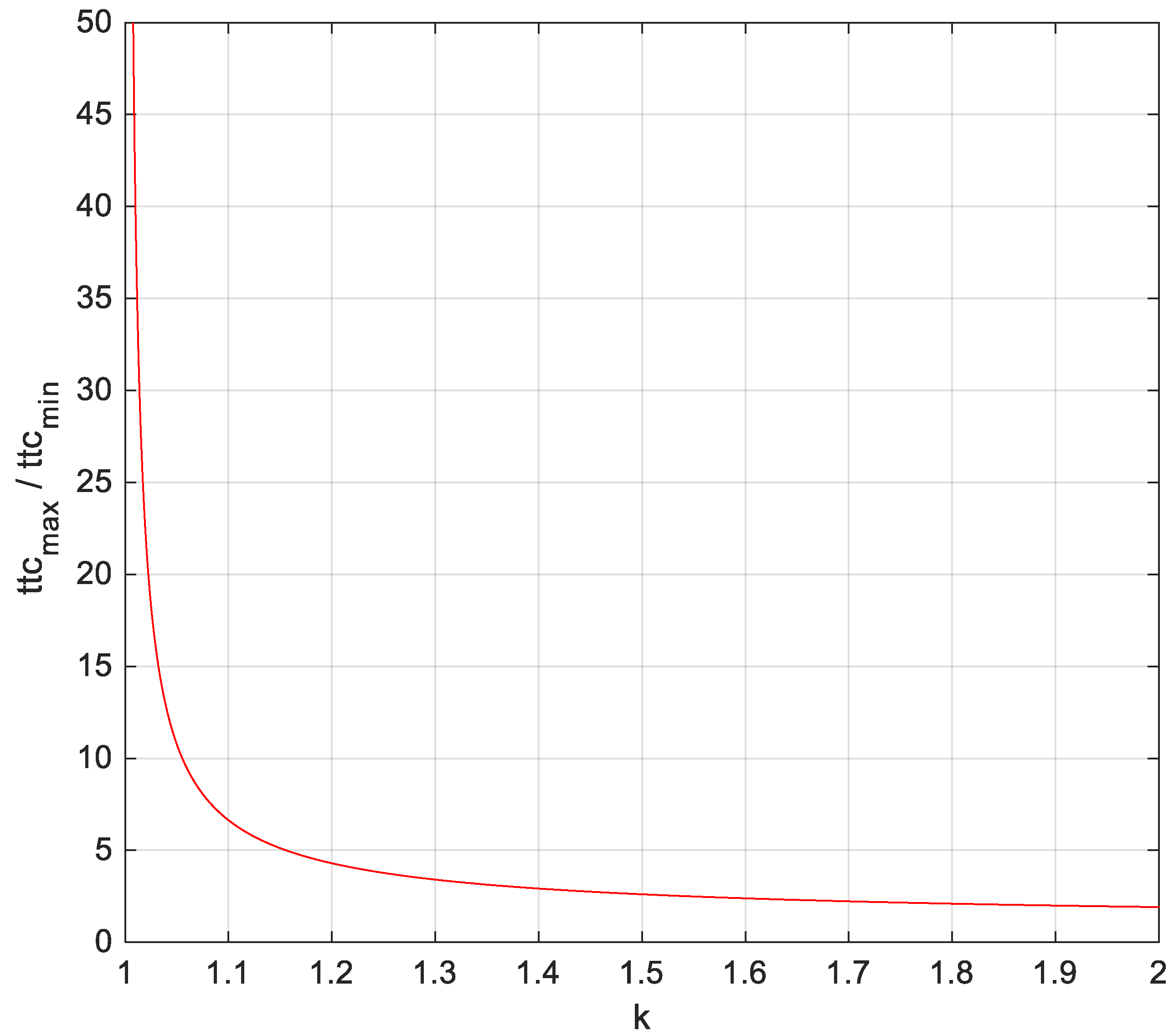
  • The size of the field of view to be monitored in the horizontal plane (azimuth) can be reduced when the ownship is faster than the obstacle; when this is not true, for a given obstacle declaration range, it is possible to adapt the surveillance rate to the variation of time to collision within the FOV.
  • As concerns the vertical plane (elevation), imposing constraints on flight path angles allows for a reduction of the required FOV in elevation in the case of “fast encounters” (approaching trajectories) for any velocity ratio. In the case of “slow encounters” (converging trajectories), constraining only flight path angles does not allow a reduction of the vertical FOV to be surveilled unless proper intervals are also established for aircraft speeds. Defining limited speed ranges, conflicts are generated at large elevation angles but are characterized by low closure rates.
  • Regarding the dependence of closest point of approach estimates on sensing accuracy in near-collision conditions for given tcpa, the highest sensitivity concerns the uncertainties on azimuth and elevation angular rates.
  • The variation of closure rate within the field of view (i.e., its reduction at increasing azimuth angles) changes the declaration range requirement as well as the impact of sensing errors, which can be exploited to relax, on a statistically consistent basis, the sensing requirements.
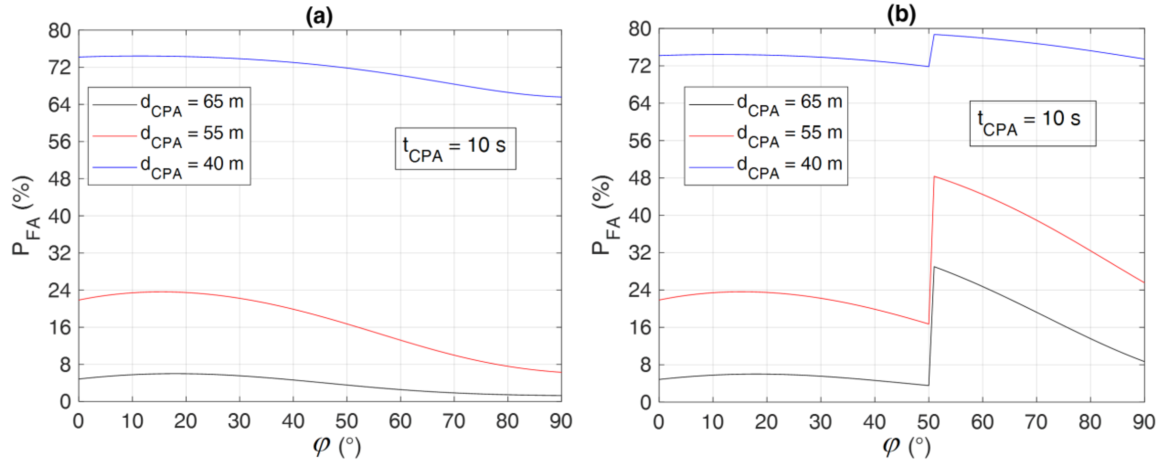
  • Numerical simulations of conflict conditions in horizontal scenarios quantitatively demonstrated that a “low-level” radar (i.e., with limited declaration range and azimuth rate accuracy) can be used to monitor lateral encounters (i.e., with intruder azimuth angles larger than 50°) with comparable performance in terms of missed and false conflict detection probabilities to a “high-level” radar handling frontal and quasi-frontal encounters.
The framework provided by the paper can be useful within different scenarios. First, the derived tools can be used to relax, on an analytical basis, the sensing requirements in lateral geometries, accounting for the traffic that may be encountered in different airspace scenarios. Second, more generally, the framework can be used to support the design and development of space–time adaptive sensing systems, where sensing resources are continuously optimized in view of target safety levels required for non-cooperative collision avoidance. Third, the approach can be useful to define ad hoc flight rules in the very low level airspace, fostering an integrated approach to the definition of sensing requirements, safety levels, and flight rules for autonomous flight. Indeed, compared with purely numerical strategies, the analytical approach is very efficient in the exploration of technological and regulatory trade-offs. Future works will aim at analyzing full 3D conflict scenarios, as well as developing adaptive sensing concepts to be tested in simulations and in-flight experiments. In addition, the framework will be applied to specific use cases and airspace scenarios to support the design of sense-and-avoid systems.

Author Contributions

Conceptualization, G.F. and R.O.; methodology, G.F. and R.O.; software, G.F. and R.O.; validation, G.F. and R.O.; formal analysis, G.F. and R.O; investigation, G.F. and R.O; resources, G.F.; data curation, R.O.; writing—original draft preparation, G.F. and R.O; writing—review and editing, G.F. and R.O; visualization, G.F. and R.O; supervision, G.F.; project administration, G.F.; funding acquisition, G.F. All authors have read and agreed to the published version of the manuscript.

Funding

This research received no external funding.

Data Availability Statement

Data sharing not applicable.

Acknowledgments

This research was carried out in the frame of project “CREATEFORUAS”, funded within Programme PRIN by the Italian Ministry of Education, University, and Research.

Conflicts of Interest

The authors declare no conflict of interest.

References

  1. Fasano, G.; Accardo, D.; Moccia, A.; Maroney, D. Sense and avoid for unmanned aircraft systems. IEEE Aerosp. Electron. Syst. Mag. 2016, 31, 82–110. [Google Scholar] [CrossRef]
  2. Zeitlin, A. Performance tradeoffs and the development of standards. In Sense and Avoid in UAS: Research and Applications, 1st ed.; Angelov, P., Ed.; Wiley: New York, NY, USA, 2012; Chapter 2. [Google Scholar]
  3. Fasano, G.; Accardo, D.; Tirri, A.E.; Moccia, A.; De Lellis, E. Radar/electro-optical data fusion for non-cooperative UAS sense and avoid. Aerosp. Sci. Technol. 2015, 46, 436–450. [Google Scholar] [CrossRef]
  4. Kotegawa, T. Proof-of-concept airborne sense and avoid system with ACAS-XU flight test. IEEE Aerosp. Electron. Syst. Mag. 2016, 31, 53–62. [Google Scholar] [CrossRef]
  5. UAS Traffic Management (UTM) Project Technical Interchange Meeting (TIM). Available online: https://nari.arc.nasa.gov/events/utm2021tim/ (accessed on 23 August 2023).
  6. Barrado, C.; Boyero, M.; Brucculeri, L.; Ferrara, G.; Hately, A.; Hullah, P.; Martin-Marrero, D.; Pastor, E.; Rushton, A.P.; Volkert, A. U-Space Concept of Operations: A Key Enabler for Opening Airspace to Emerging Low-Altitude Operations. Aerospace 2020, 7, 24. [Google Scholar] [CrossRef]
  7. Jamoom, M.B.; Joerger, M.; Pervan, B. Unmanned aircraft system sense-and-avoid integrity and continuity risk. J. Guid. Control Dyn. 2016, 39, 498–509. [Google Scholar] [CrossRef]
  8. Huh, S.; Cho, S.; Jung, Y.; Shim, D.H. Vision-based sense-and-avoid framework for unmanned aerial vehicles. IEEE Trans. Aerosp. Electron. Syst. 2015, 51, 3427–3439. [Google Scholar] [CrossRef]
  9. Opromolla, R.; Fasano, G. Visual-based obstacle detection and tracking, and conflict detection for small UAS sense and avoid. Aerosp. Sci. Technol. 2021, 119, 107167. [Google Scholar] [CrossRef]
  10. Ma, Z.; Yao, W.; Niu, Y.; Lin, B.; Liu, T. UAV low-altitude obstacle detection based on the fusion of LiDAR and camera. Auton. Intell. Syst. 2021, 1, 12. [Google Scholar] [CrossRef]
  11. Jilkov, V.P.; Ledet, J.H.; Li, X.R. Multiple model method for aircraft conflict detection and resolution in intent and weather uncertainty. IEEE Trans. Aerosp. Electron. Syst. 2018, 55, 1004–1020. [Google Scholar] [CrossRef]
  12. Mishra, C.; Maskell, S.; Au, S.K.; Ralph, J.F. Efficient estimation of probability of conflict between air traffic using Subset Simulation. IEEE Trans. Aerosp. Electron. Syst. 2019, 55, 2719–2742. [Google Scholar] [CrossRef]
  13. Lies, W.A.; Narula, L.; Iannucci, P.; Humphreys, T. Long Range, Low SWaP-C FMCW Radar. IEEE J. Sel. Top. Signal Process. 2021, 15, 1030–1040. [Google Scholar] [CrossRef]
  14. Weinert, A.; Campbell, D.; Vela, A.; Schuldt, D.; Kurucar, J. Well-clear recommendation for small unmanned aircraft systems based on unmitigated collision risk. J. Air Transp. 2018, 26, 113–122. [Google Scholar] [CrossRef]
  15. Jones, J.C.; Panken, A.; Lopez, J.A. Surrogate-Based Optimization for Radar Surveillance Requirements to Support RWC and CA for Unmanned Aircraft. In Proceedings of the 2018 IEEE/AIAA 37th Digital Avionics Systems Conference (DASC), London, UK, 23–27 September 2018. [Google Scholar]
  16. Kochenderfer, M.J.; Edwards, M.W.; Espindle, L.P.; Kuchar, J.K.; Griffith, J.D. Airspace encounter models for estimating collision risk. J. Guid. Control Dyn. 2010, 33, 487–499. [Google Scholar] [CrossRef]
  17. Lee, H.; Park, B.; Lee, H. Analysis of ADS-B Trajectories in the Republic of Korea with DAA Well Clear Metrics. In Proceedings of the 2018 IEEE/AIAA 37th Digital Avionics Systems Conference (DASC), London, UK, 23–27 September 2018. [Google Scholar]
  18. Underhill, N.; Weinert, A. Applicability and Surrogacy of Uncorrelated Airspace Encounter Models at Low Altitudes. J. Air Transp. 2021, 29, 137–141. [Google Scholar] [CrossRef]
  19. Fasano, G.; Accardo, D.; Tirri, A.E.; Moccia, A. Experimental analysis of onboard non-cooperative sense and avoid solutions based on radar, optical sensors, and data fusion. IEEE Aerosp. Electron. Syst. Mag. 2016, 31, 6–14. [Google Scholar] [CrossRef]
  20. Edwards, M.W.M.; Mackay, J.K. Determining Required Surveillance Performance for Unmanned Aircraft Sense and Avoid. In Proceedings of the AIAA Aviation Forum, Denver, CO, USA, 5–9 June 2017. [Google Scholar]
  21. Opromolla, R.; Fasano, G.; Accardo, D. Perspectives and sensing concepts for small UAS sense and avoid. In Proceedings of the 2018 IEEE/AIAA 37th Digital Avionics Systems Conference (DASC), London, UK, 23–27 September 2018; pp. 1–10. [Google Scholar]
  22. Opromolla, R.; Fasano, F.; Accardo, D. Conflict Detection Performance of Non-Cooperative Sensing Architectures for Small UAS Sense and Avoid. In Proceedings of the 2019 Integrated Communications, Navigation and Surveillance Conference (ICNS), Herndon, VA, USA, 9–11 April 2019; pp. 1–12. [Google Scholar]
  23. Vitiello, F.; Causa, F.; Opromolla, R.; Fasano, G. Improved Sensing Strategies for Low Altitude Non Cooperative Sense and Avoid. In Proceedings of the 2021 IEEE/AIAA 40th Digital Avionics Systems Conference (DASC), San Antonio, TX, USA, 3–7 October 2021; pp. 1–10. [Google Scholar]
  24. Sharma, P.; Ochoa, C.A.; Atkins, E.M. Sensor constrained flight envelope for urban air mobility. In Proceedings of the AIAA SciTech 2019 Forum, San Diego, CA, USA, 7–11 January 2019; p. 949. [Google Scholar]
  25. Wikle, J.K.; McLain, T.W.; Beard, R.W.; Sahawneh, L.R. Minimum required detection range for detect and avoid of unmanned aircraft systems. J. Aerosp. Inf. Syst. 2017, 14, 351–372. [Google Scholar] [CrossRef]
  26. Euliss, G.; Christiansen, A.; Athale, R. Analysis of laser-ranging technology for sense and avoid operation of unmanned aircraft systems: The tradeoff between resolution and power. In Proceedings of the SPIE Defense and Security Symposium, Orlando, FL, USA, 16 April 2008. [Google Scholar]
  27. Schaefer, R. A standards-based approach to sense-and-avoid technology. In Proceedings of the AIAA 3rd “Unmanned Unlimited” Technical Conference, Workshop and Exhibit, Chicago, IL, USA, 20–23 September 2004; p. 6420. [Google Scholar]
  28. Utt, J.; McCalmont, J.; Deschenes, M. Development of a sense and avoid system. In Proceedings of the Infotech@ Aerospace, Arlington, VA, USA, 26–29 September 2005; p. 7177. [Google Scholar]
Figure 1. 2D (horizontal) collision geometry.
Drones 07 00621 g001
Figure 2. Size of azimuth FOV in which collisions may occur for obstacles slower than the UAV (k < 1).
Drones 07 00621 g002
Figure 3. Time-to-collision ratio as a function of k (for αLIM equal to −10°). The case of k > 1 corresponds to intruders that are faster than the ownship.
Drones 07 00621 g003
Figure 4. Geometry for vertical FOV analysis (fixed-wing aircraft depicted only as an example case).
Drones 07 00621 g004
Figure 5. Obstacle elevation angles and closing rate in collision conditions as a function of obstacle flight path angle (γUAV assumed equal to 10°, fast encounter geometry). The black arrow indicates the direction along which k increases.
Drones 07 00621 g005
Figure 6. Obstacle elevation angles and closing rate in collision conditions as a function of obstacle flight path angle (γUAV assumed equal to 10°, slow encounter geometry). The black arrow indicates the direction along which k increases.
Drones 07 00621 g006
Figure 7. Geometric interpretation of collision conditions that are generated when γUAV = γmax. As in the paper text, XUAV and YUAV, respectively, identify the axes parallel and perpendicular to the UAV velocity vector; blue arrows indicate various possible angular positions of the intruder. For each condition, the ownship velocity and the intruder velocity vector leading to a collision are depicted in red and green, respectively.
Drones 07 00621 g007
Figure 8. Three-dimensional collision geometry (VA and VB do not belong to the same plane).
Drones 07 00621 g008
Figure 9. Two-dimensional evaluation of the probability of missed detection PMD,track_acc based on the statistical distribution of dCPA components. The blue point represents the true CPA. The value of PMD,track_acc is evaluated as the integral of the distribution outside the shaded rectangle identified by the assumed thresholds.
Drones 07 00621 g009
Figure 10. Two-dimensional (horizontal) geometry to derive the variation of range rate as a function of the azimuth angle for a given dCPA.
Drones 07 00621 g010
Figure 11. Histogram representing the statistical distribution of dCPA,hor (left) and dCPA,ver (right) for 1,000,000 random simulations of the scenario described by the obstacle state parameter and firm tracking uncertainties reported in Table 2. The y-axes of the plots report the number of instances in which dCPA,hor and dCPA,ver assume the value in the corresponding bin of the x-axis.
Drones 07 00621 g011
Figure 12. Error in the evaluation of the dCPA uncertainties after firm tracking using the approximated derivatives from Section 2.2.
Drones 07 00621 g012
Figure 13. Example of 2D (horizontal) collision geometry considered for the numerical analysis presented in this subsection.
Drones 07 00621 g013
Figure 14. PMD as a function of φ and dCPA for the SAA architectures SAARADAR-1 (a) and SAARADAR-2 (b). The tCPA is 20 s.
Drones 07 00621 g014
Figure 15. PMD as a function of φ and dCPA, for the SAA architectures SAARADAR-1 (a) and SAARADAR-2 (b). The tCPA is 10 s.
Drones 07 00621 g015
Figure 16. PFA as a function of φ and dCPA for the SAA architectures SAARADAR-1 (a) and SAARADAR-2 (b). The tCPA is 20 s.
Drones 07 00621 g016
Figure 17. PFA evaluated considering only the effect of sensing accuracy as a function of φ and dCPA for the SAA architectures SAARADAR-1 (a) and SAARADAR-2 (b). The tCPA is 20 s.
Drones 07 00621 g017
Figure 18. PFA as a function of φ and dCPA for the SAA architectures SAARADAR-1 (a) and SAARADAR-2 (b). The tCPA is 10 s.
Drones 07 00621 g018
Table 1. List of derivatives of dCPA,hor and dCPA,ver with respect to ( r , φ , θ , r ˙ , φ ˙ , θ ˙ ) evaluated in the case of a near-collision encounter, and their orders of magnitude.
Horizontal DerivativeApproximated Value from (42)O(-)Vertical DerivativeApproximated Value from (43)O(-)
d C P A , h o r r 2 r r ˙ θ ˙ 2 sin θ 2 + φ ˙ 2 cos θ 2 ε d C P A , v e r r 2 r r ˙ θ ˙ cos θ ε cos θ
d C P A , h o r φ 00 d C P A , v e r φ 00
d C P A , h o r θ r 2 sin 2 θ 2 r ˙ θ ˙ 2 sin θ 2 + φ ˙ 2 cos θ 2 θ ˙ 2 φ ˙ 2 r ˙ t C P A ε sin 2 θ d C P A , v e r θ r 2 r ˙ θ ˙ sin θ r ˙ t C P A ε sin θ
d C P A , h o r r ˙ r 2 r ˙ 2 θ ˙ 2 sin θ 2 + φ ˙ 2 cos θ 2 ε t C P A d C P A , v e r r ˙ r 2 r ˙ 2 θ ˙ cos θ ε t C P A cos θ
d C P A , h o r φ ˙ r 2 φ ˙ cos θ 2 r ˙ θ ˙ 2 sin θ 2 + φ ˙ 2 cos θ 2 r ˙ t C P A 2 cos θ 2 d C P A , v e r φ ˙ 00
d C P A , h o r θ ˙ r 2 θ ˙ sin θ 2 r ˙ θ ˙ 2 sin θ 2 + φ ˙ 2 cos θ 2 r ˙ t C P A 2 sin θ 2 d C P A , v e r θ ˙ r 2 r ˙ cos θ r ˙ t C P A 2 cos θ 2
Table 2. Relative motion scenario: true obstacle state parameters and corresponding firm tracking uncertainties.
R (m)φ (°)θ (°) r ˙ (m/s) φ ˙ (°/s) θ ˙ (°/s)
10005010−500.020.01
σ r (m) σ φ (°) σ θ (°) σ r ˙ (m/s) σ φ ˙ (°/s) σ θ ˙ (°/s)
102110.20.1
Table 3. Comparison between the simulated dCPA uncertainties and the ones obtained applying the approximated derivatives from Section 2.2.
σdCPA,hor,sim (m)σdCPA,ver,sim (m)σdCPA,hor,app (m)σdCPA,ver,app (m)
68.4434.1767.7234.38
Table 4. Firm tracking performance for the selected radar-based architectures for SAA.
Intruder Track. State Estimation UncertaintySAARADAR-1SAARADAR-2
0° ≤ φ < 90°
“High-Level” Radar
0° ≤ φ < 50°
“High-Level” Radar
50° ≤ φ < 90°
“Low-Level” Radar
σ r (m)3.253.253.25
σ r ˙ (m/s)0.9000.9000.900
σ φ ˙ (°/s)0.300.300.60
μ r , f t (m)400400300
σ r , f t (m)505040
Disclaimer/Publisher’s Note: The statements, opinions and data contained in all publications are solely those of the individual author(s) and contributor(s) and not of MDPI and/or the editor(s). MDPI and/or the editor(s) disclaim responsibility for any injury to people or property resulting from any ideas, methods, instructions or products referred to in the content.

