
Distributed Control for Multi-Robot Interactive Swarming Using Voronoi Partioning †


Abstract
:1. Introduction
- Proposition of a distributed control algorithm enabling non-rigid motion for human-multi-robot swarming in cluttered environments.
- Design of a purely geometric approach applied by each robot to define distributively a reference point to be tracked inside its Voronoi cell, accounting for other robots and obstacles (collision avoidance), as well as human operators (collision avoidance and other possible interactions, see below).
- Decoupling between the mechanisms of obstacle avoidance and collision avoidance. This allows to reduce the design complexity when accounting for obstacles, as opposed to navigation functions for example, and to render the gain tuning more straightforward.
- Possibility to handle different modes of interactions between human operator and robots of the swarm. These modes of interactions correspond to practical problems of interest which are autonomous waypoint navigation, velocity-guided motion and follow a localized operator.
- Implementation and real-world field experiments in indoor and outdoor environments with self-localized ground mobile robots and human operator, in presence of various obstacles.
2. Swarm Control Method
2.1. Problem Definition
- An Autonomous mode, in which the swarm has to follow autonomously a predefined path at a given nominal speed. Examples of tasks that can be performed with this mode are transfers of equipment or injured people between two locations. Other tasks could be the persistent surveillance of zones in order to detect abnormal events, by making the UGVs autonomously and repeatedly move along a surveillance path composed of predefined waypoints.
- A Velocity-Guided mode, where the swarm follows a predefined path at the same speed as a human operator. In other words, the desired positions and orientations of the robots with respect to the waypoints are the same as in the Autonomous mode, but the velocity to reach them is defined by the motion of a human operator.
- A Follow mode, where the current waypoint to be tracked is defined with respect to the localized operator and also takes into account the positions of all the robots. Note that the human operator could be replaced by a tele-operated robot or a virtual point to obtain a platooning behavior, using the same underlying control algorithm.
2.2. Algorithm Description
- Step 1: Voronoi partitioning
- Step 2: Attraction to waypoint
- Special cases or : During the mission, the number of neighbors of a robot may change, temporarily or definitively, e.g., due to loss of communication links, loss of robots, etc. If at a given instant, Robot i has zero or one neighbor, one additional step is performed before the standard algorithm. This step is described in Appendix A.
- Step 3: Obstacle avoidance
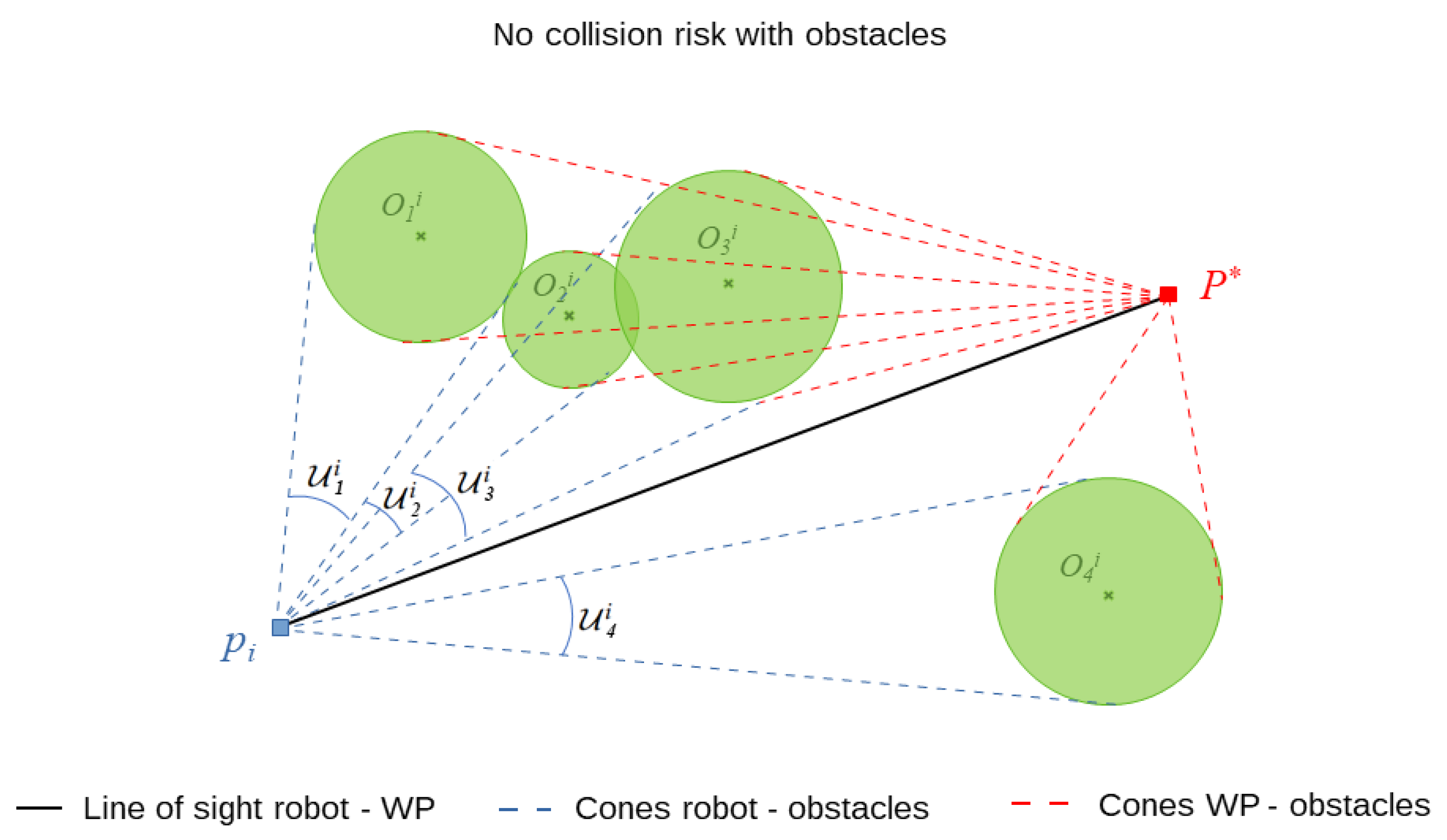
- If not, there is no collision risk with any of the obstacles, and direct straight motion to the waypoint is safe for the robot (as described in Figure 3). The attraction point computed at Step 2 is still valid and the algorithm proceeds to the next step.
- If there is at least one obstacle with collision risk, the cone of this obstacle is considered. It is enlarged step by step by considering adjacent and intersecting cones related to other obstacles, so as to obtain a larger cone containing a cluster of the obstacles with collision risk for robot i. An example is provided on the left part of Figure 4: the collision cone of obstacle is merged with the intersecting collision cone of obstacle , which is further merged with collision cone of obstacle . This iterative procedure is stopped as there are no other intersection collision cones. The resulting cone is depicted by dashed blue lines. The same procedure is repeated to build another cone , but this time by considering the waypoint as vertex. The two intersection points and between these bounding cones are then computed. They correspond to two intermediate target points for the robot, each of them defining a possible obstacle-free path towards the waypoint. Some heuristics are used at this stage to select the shortest among the two available paths. The target point corresponding to the selected path is considered, instead of the waypoint, to compute a new attraction point , in the same way as in Step 2. This new attraction point replaces the one computed in Step 2 and is used instead for the rest of the algorithm.
- Step 4: Collision avoidance with other agents
- Step 5: Computation of reference
2.3. Waypoint and Velocity Management
- Selfish: each robot has to validate its current waypoint (given a parameterized validation distance ), then it moves to the next waypoint in the list. This way, all the robots will cross each waypoint and stay close to the path. On the other hand, this does not impose any waiting behavior between the robots.
- First: when a robot is the first to validate the current waypoint, all robots head to the next waypoint in the list by sharing its index. This strategy can be applied in large environments where deviation from the path can be allowed. There is also no waiting behavior around each waypoint in this case, however the UGVs always agree on and head towards the same current waypoint.
- WaitForAll: in this strategy, the waypoint is validated only if each robot either gets closer to the waypoint than the validation distance or if it is near the avoidance distance of another robot () which validates one of these conditions. This is a more collective behavior, where all robots should wait for the others before heading to the next waypoint. This also creates a kind of validation chain between the UGVs, which is a useful feature for large swarms where all the UGVs cannot get closer to the waypoint than the validation distance because of the collision avoidance constraints.
2.4. Main Properties of the Algorithm
2.4.1. Safety Regions
2.4.2. Flexibility and Pattern of the Swarm
2.4.3. Decentralized Algorithm for Robustness to Robot Failure and Communication Loss
3. System Architecture
3.1. Architecture
3.2. Local Mapping from Embedded Depth Sensors
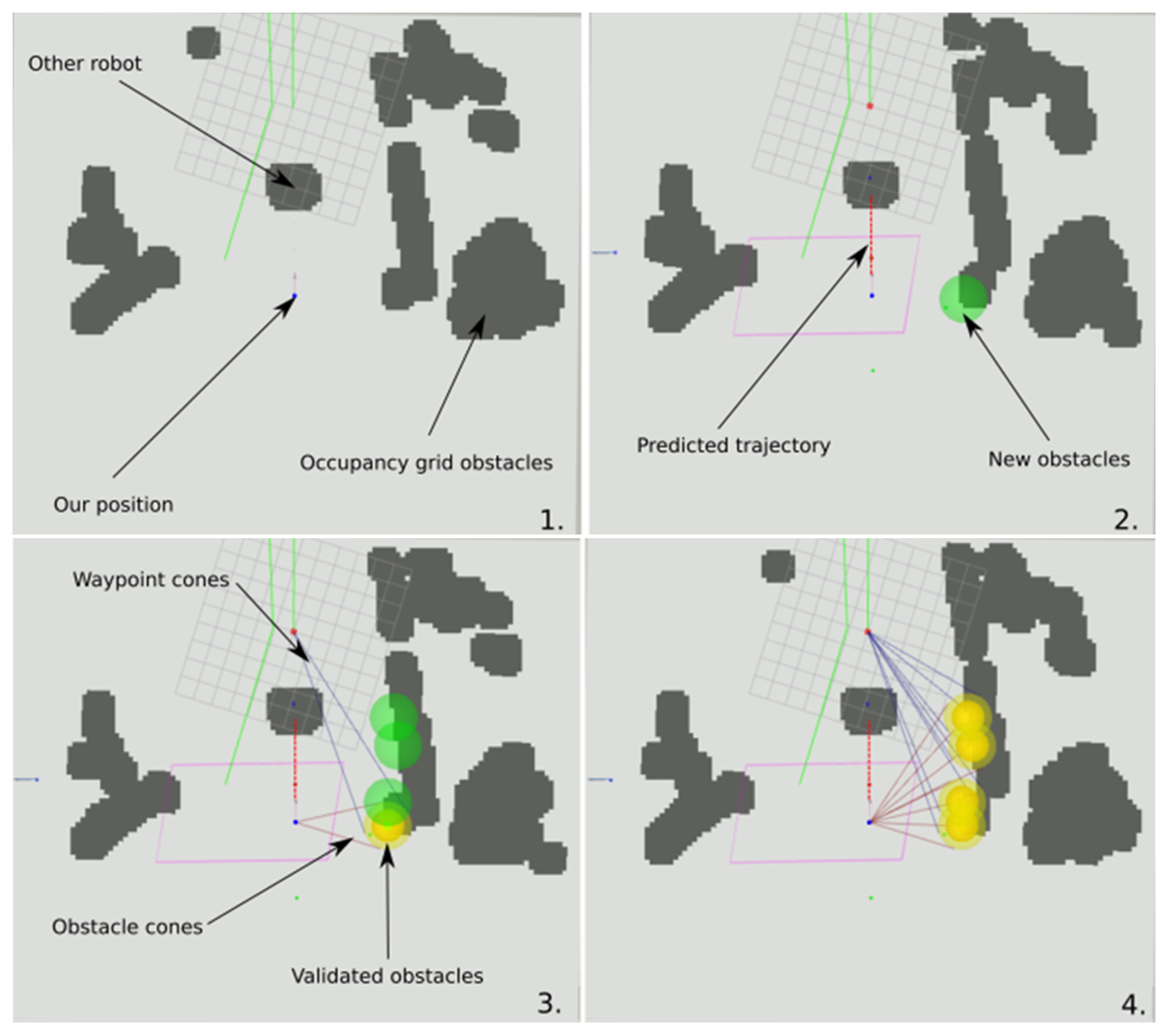
- Obstacle initializationThe local map does not keep track of all obstacles detected by the sensor but focuses only on the most threatening ones. Those are obstacles which are closest to the current position or to the future position along the predicted trajectory. When a possible new obstacle is found, we add it to the local map if it is not already tracked. The created obstacle is a disk of radius (parameterized safety distance) centered on the grid point of a threatening obstacle, displayed in green in Figure 8 (sub-figures 2 and 3). All the new obstacles are created and tracked but not taken into account for avoidance immediately. This requires that the corresponding location has been seen as occupied a certain number of times in successive occupancy grids to filter out measurement artefacts (vegetation, dust, …).
- Obstacle life cycleWhen a new occupancy grid becomes available, each tracked obstacle is projected in the occupancy grid to check if it is still present. If this is the case, we increase the number of observations of this obstacle and reset the last time it has been seen. When an obstacle reaches a certain number of observations (set to 3 in our experiments), it is validated and considered for obstacle avoidance (in yellow in the map). In this algorithm, the radius of the obstacle is enlarged by an additional distance to take into account the size of the robot or the drift of localization (in light yellow on the map pictures). This number of observations is saturated at a given threshold (set to 100 in our experiments) to be able to remove obstacles that have been seen during a long period at a given location but have moved away afterwards.
- Obstacle removalAfter new obstacles are initialized, tracked and updated, obstacle removal is carried out. This process is based on the number of views and the last time an obstacle has been seen. When an obstacle is not seen anymore: after a certain amount of time passed from the last time it has been seen (set to 1 s in our experiments), the number of observations is decremented. When the number of observations reaches the minimum-view threshold, the obstacle is removed from the map. This process allows to keep track of an obstacle that has been seen for an extended period of time while allowing for a fast removal of an obstacle that has been seen just a short number of times. This process will also remove the obstacles that have been initialized but never seen again (validated).
- Occupancy grid pre-filteringDue to the multi-agent context, the input occupancy grid is pre-processed to remove views of the other agents (UGV or operator) such that they are not considered as obstacles, since they are moving and taken into account directly at Step 4 of the main algorithm. The global positions of the other robots and of the operator are projected in the local grid. All obstacle cells present in a given radius (chosen to be consistent with the robot dimensions and localization uncertainty) around these positions are then removed. This can be seen in Figure 8, where the spot in front of the robot currently building the map is at the location of another robot but is not considered as an obstacle.
4. Experimental Results
- 3 Robotnik Summit XL UGVs of mass 65 kg and base dimension 72 × 61 cm, equipped with a calibrated stereo-rig of IDS UI-3041LE cameras (baseline of 35 cm, running at 20 Hz) and an embedded Intel-NUC CPU.
- 1 operator Portable Localization Kit comprising an Intel RealSense d455 depth camera and a Intel-NUC CPU.
- A standard WiFi network connecting all the embedded computers and a ground station for mission supervision and visualization. Transmission of the positions between the robots was carried out using Ultra Wideband (UWB) DW1000 radio modules in a similar way as in [37].
- Algorithm tuning
- Collisions: m, ,
- Attraction: m,
- Repulsion: m,
- Mirrors: m
- Validation: m,
- Obstacles: m, m
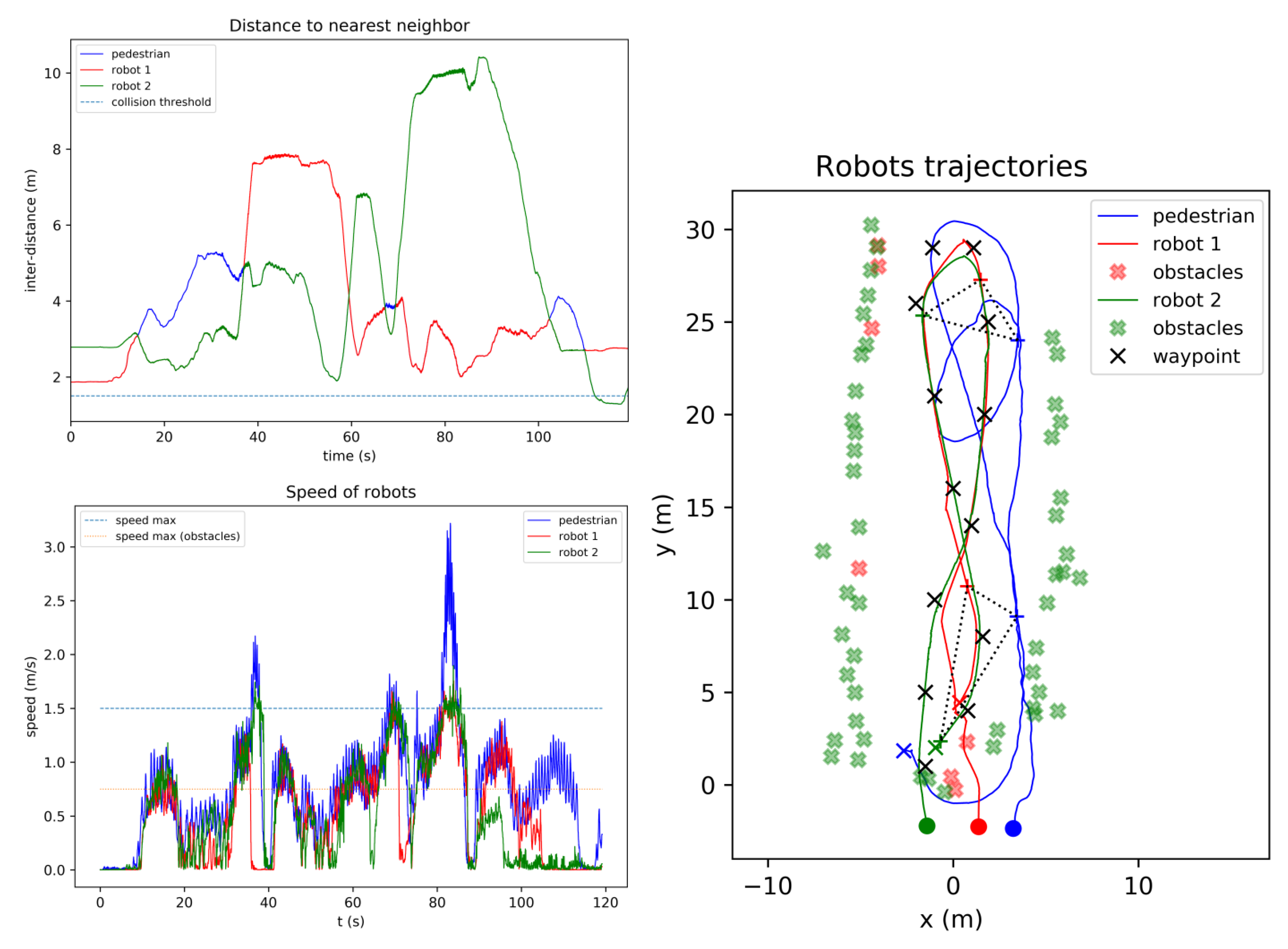
4.1. Autonomous Mode
4.2. Velocity-Guided Mode
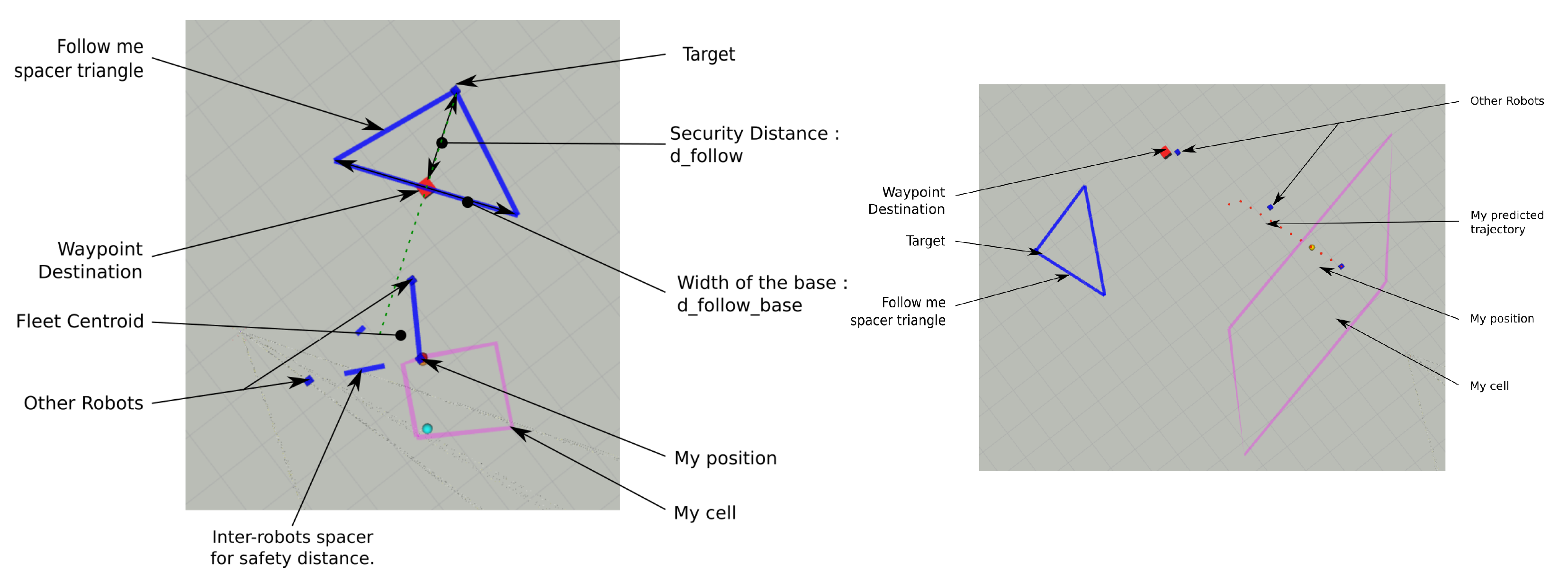
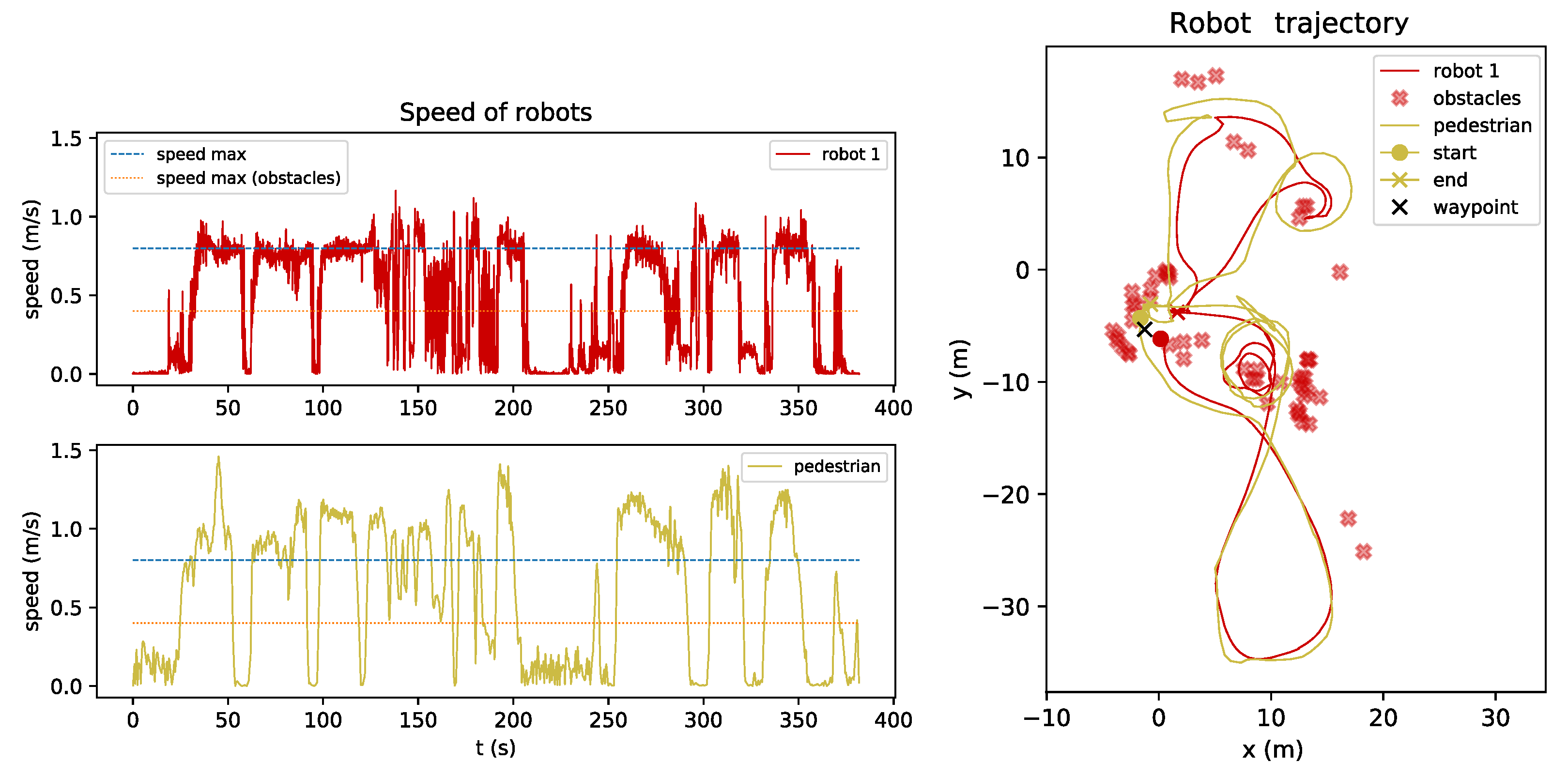
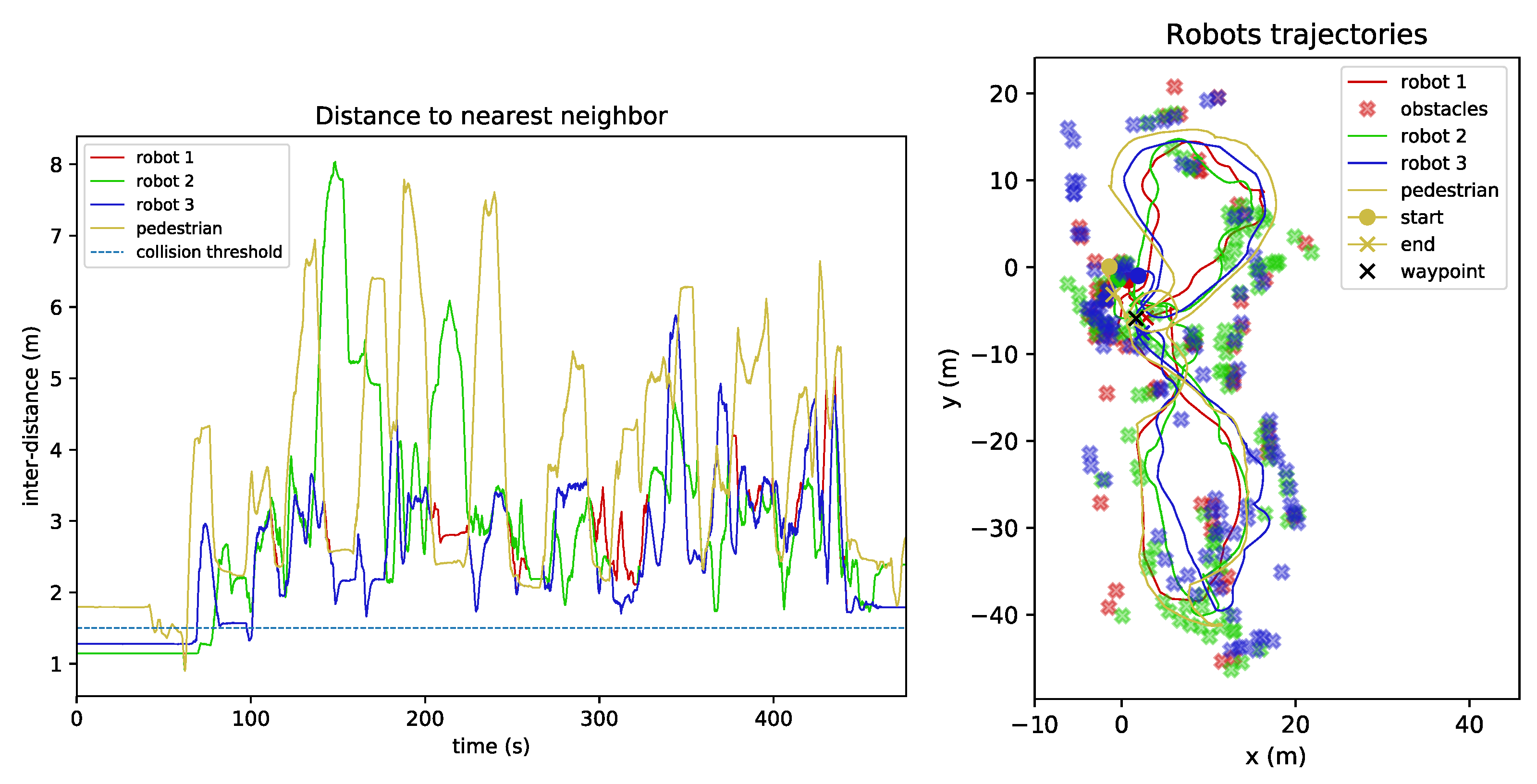
4.3. Follow Mode
- The minimal distance to which a robot could approach the target.
- The parameter, which has an influence on the shape of the robots formation behind the target. If the base length is short, the robots will be more in line, while if it is larger a triangular shape will emerge. A standard tuning was chosen equal to .
5. Conclusions and Perspectives
Author Contributions
Funding

Conflicts of Interest
Appendix A
- If , Robot i has no neighbors. In this case, the robot only executes Steps 2 & 3 for obstacle avoidance and does not compute the Voronoi partitioning and collision avoidance with neighbors. Finally, the robot will track the reference points .
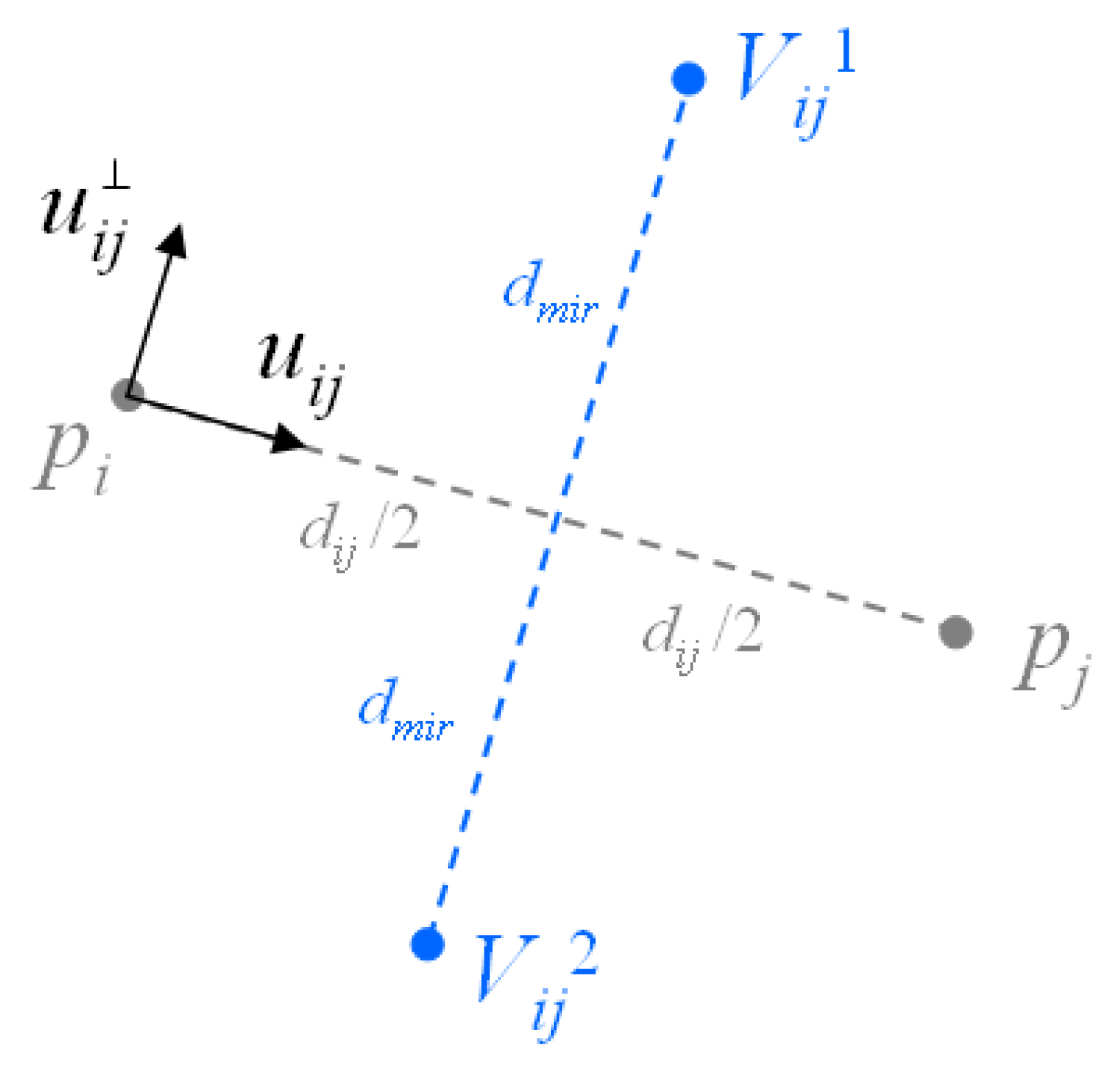
- If , Robot i has only one neighbor. In this case, the Voronoi cell obtained in Step 1 will be degenerated. To avoid this problem, if , two virtual robots are defined as follows and their indices are added to .
References
- Moussa, M.; Beltrame, G. On the robustness of consensus-based behaviors for robot swarms. Swarm Intell. 2020, 14, 205–231. [Google Scholar] [CrossRef]
- Adoni, W.Y.H.; Lorenz, S.; Fareedh, J.S.; Gloaguen, R.; Bussmann, M. Investigation of Autonomous Multi-UAV Systems for Target Detection in Distributed Environment: Current Developments and Open Challenges. Drones 2023, 7, 263. [Google Scholar] [CrossRef]
- Murray, R.M. Recent research in cooperative control of multivehicle systems. J. Dyn. Syst. Meas. Control 2007, 129, 571–583. [Google Scholar] [CrossRef]
- Mesbahi, M.; Egerstedt, M. Graph Theoretic Methods in Multi-Agent Networks; Princeton University Press: Princeton, NJ, USA, 2010. [Google Scholar]
- Ren, W.; Beard, R.W. Distributed Consensus in Multi-Vehicle Cooperative Control; Springer: Berlin/Heidelberg, Germany, 2010. [Google Scholar] [CrossRef]
- Canepa, D.; Potop-Butucaru, M.G. Stabilizing Flocking via Leader Election in Robot Networks. In Stabilization, Safety, and Security of Distributed Systems; Springer: Berlin/Heidelberg, Germany, 2007; pp. 52–66. [Google Scholar] [CrossRef]
- Balch, T.; Arkin, R.C. Behavior-based formation control for multirobot teams. IEEE Trans. Robot. Autom. 1998, 14, 926–939. [Google Scholar] [CrossRef]
- Lee, G.; Chwa, D. Decentralized behavior-based formation control of multiple robots considering obstacle avoidance. Intell. Serv. Robot. 2018, 11, 127–138. [Google Scholar] [CrossRef]
- Zhou, D.; Wang, Z.; Schwager, M. Agile coordination and assistive collision avoidance for quadrotor swarms using virtual structures. IEEE Trans. Robot. 2018, 34, 916–923. [Google Scholar] [CrossRef]
- Kahn, A.; Marzat, J.; Piet-Lahanier, H. Formation flying control via elliptical virtual structure. In Proceedings of the IEEE International Conference on Networking, Sensing and Control, Paris-Evry, France, 10–12 April 2013; pp. 158–163. [Google Scholar] [CrossRef]
- Lafferriere, G.; Williams, A.; Caughman, J.; Veerman, J.J.P. Decentralized control of vehicle formations. Syst. Control Lett. 2005, 54, 899–910. [Google Scholar] [CrossRef]
- Oh, K.K.; Park, M.C.; Ahn, H.S. A survey of multi-agent formation control. Automatica 2015, 53, 424–440. [Google Scholar] [CrossRef]
- Fathian, K.; Rachinskii, D.I.; Spong, M.W.; Summers, T.H.; Gans, N.R. Distributed formation control via mixed barycentric coordinate and distance-based approach. In Proceedings of the American Control Conference, Philadelphia, PA, USA, 10–12 July 2019; pp. 51–58. [Google Scholar] [CrossRef]
- Cheah, C.C.; Hou, S.P.; Slotine, J.J.E. Region-based shape control for a swarm of robots. Automatica 2009, 45, 2406–2411. [Google Scholar] [CrossRef]
- Strandburg-Peshkin, A.; Twomey, C.R.; Bode, N.W.; Kao, A.B.; Katz, Y.; Ioannou, C.C.; Rosenthal, S.B.; Torney, C.J.; Wu, H.S.; Levin, S.A.; et al. Visual sensory networks and effective information transfer in animal groups. Curr. Biol. 2013, 23, R709–R711. [Google Scholar] [CrossRef]
- Kolpas, A.; Busch, M.; Li, H.; Couzin, I.D.; Petzold, L.; Moehlis, J. How the Spatial Position of Individuals Affects Their Influence on Swarms: A Numerical Comparison of Two Popular Swarm Dynamics Models. PLoS ONE 2013, 8, e58525. [Google Scholar] [CrossRef] [PubMed]
- Cortes, J.; Martinez, S.; Karatas, T.; Bullo, F. Coverage control for mobile sensing networks. IEEE Trans. Robot. Autom. 2004, 20, 243–255. [Google Scholar] [CrossRef]
- Guruprasad, K.R.; Dasgupta, P. Distributed Voronoi partitioning for multi-robot systems with limited range sensors. In Proceedings of the IEEE/RSJ International Conference on Intelligent Robots and Systems, Vilamoura, Portugal, 7–12 October 2012; pp. 3546–3552. [Google Scholar] [CrossRef]
- Hatleskog, J.; Olaru, S.; Hovd, M. Voronoi-based deployment of multi-agent systems. In Proceedings of the IEEE Conference on Decision and Control, Miami, FL, USA, 17–19 December 2018; pp. 5403–5408. [Google Scholar] [CrossRef]
- Zhou, Z.; Zhang, W.; Ding, J.; Huang, H.; Stipanović, D.M.; Tomlin, C.J. Cooperative pursuit with Voronoi partitions. Automatica 2016, 72, 64–72. [Google Scholar] [CrossRef]
- Kouzeghar, M.; Song, Y.; Meghjani, M.; Bouffanais, R. Multi-Target Pursuit by a Decentralized Heterogeneous UAV Swarm using Deep Multi-Agent Reinforcement Learning. In Proceedings of the IEEE International Conference on Robotics and Automation, London, UK, 29 May–2 June 2023. [Google Scholar]
- Gui, J.; Yu, T.; Deng, B.; Zhu, X.; Yao, W. Decentralized Multi-UAV Cooperative Exploration Using Dynamic Centroid-Based Area Partition. Drones 2023, 7, 337. [Google Scholar] [CrossRef]
- Lindhé, M.; Ogren, P.; Johansson, K.H. Flocking with obstacle avoidance: A new distributed coordination algorithm based on Voronoi partitions. In Proceedings of the IEEE International Conference on Robotics and Automation, Barcelona, Spain, 18–22 April 2005; pp. 1785–1790. [Google Scholar] [CrossRef]
- Lindhé, M.; Johansson, K.H. A Formation Control Algorithm using Voronoi Regions. In Taming Heterogeneity and Complexity of Embedded Control; John Wiley & Sons, Ltd.: Hoboken, NJ, USA, 2013; Chapter 24; pp. 419–434. [Google Scholar] [CrossRef]
- Jiang, Q. An improved algorithm for coordination control of multi-agent system based on r-limited Voronoi partitions. In Proceedings of the IEEE International Conference on Automation Science and Engineering, Shanghai, China, 7–10 October 2006; pp. 667–671. [Google Scholar] [CrossRef]
- Bertrand, S.; Sarras, I.; Eudes, A.; Marzat, J. Voronoi-based Geometric Distributed Fleet Control of a Multi-Robot System. In Proceedings of the 16th International Conference on Control, Automation, Robotics and Vision (ICARCV), Shenzhen, China, 13–15 December 2020; pp. 85–91. [Google Scholar] [CrossRef]
- Chakravarthy, A.; Ghose, D. Obstacle avoidance in a dynamic environment: A collision cone approach. IEEE Trans. Syst. Man, Cybern. Part A Syst. Hmans 1998, 28, 562–574. [Google Scholar] [CrossRef]
- Sunkara, V.; Chakravarthy, A.; Ghose, D. Collision Avoidance of Arbitrarily Shaped Deforming Objects Using Collision Cones. IEEE Robot. Autom. Lett. 2019, 4, 2156–2163. [Google Scholar] [CrossRef]
- Hu, J.; Wang, M.; Zhao, C.; Pan, Q.; Du, C. Formation control and collision avoidance for multi-UAV systems based on Voronoi partition. Sci. China Technol. Sci. 2020, 63, 65–72. [Google Scholar] [CrossRef]
- Moniruzzaman, M.D.; Rassau, A.; Chai, D.; Islam, S.M.S. Teleoperation methods and enhancement techniques for mobile robots: A comprehensive survey. Robot. Auton. Syst. 2022, 150, 103973. [Google Scholar] [CrossRef]
- Aggravi, M.; Sirignano, G.; Giordano, P.R.; Pacchierotti, C. Decentralized Control of a Heterogeneous Human–Robot Team for Exploration and Patrolling. IEEE Trans. Autom. Sci. Eng. 2021, 19, 3109–3125. [Google Scholar] [CrossRef]
- Sydorchuk, A. The Boost Polygon Voronoi Extensions. 2013. Available online: https://www.boost.org/doc/libs/1_60_0/libs/polygon/doc/voronoi_main.htm (accessed on 3 July 2023).
- Pereyra, E.; Araguás, G.; Kulich, M. Path planning for a formation of mobile robots with split and merge. In Proceedings of the 4th International Conference on Modelling and Simulation for Autonomous Systems, Rome, Italy, 24–26 October 2017; Springer: Berlin/Heidelberg, Germany, 2018; pp. 59–71. [Google Scholar] [CrossRef]
- Salvado, J.; Mansouri, M.; Pecora, F. Combining multi-robot motion planning and goal allocation using roadmaps. In Proceedings of the IEEE International Conference on Robotics and Automation (ICRA), Xi’an, China, 30 May–5 June 2021; pp. 10016–10022. [Google Scholar] [CrossRef]
- Fortune, S. A sweepline algorithm for Voronoi diagrams. In Proceedings of the Second Annual Symposium on Computational Geometry, Yorktown Heights, NY, USA, 2–4 June 1986; pp. 313–322. [Google Scholar]
- Bak, M.; Poulsen, N.K.; Ravn, O. Path Following Mobile Robot in the Presence of Velocity Constraints; Technical Report, Informatics and Mathematical Modelling; Technical University of Denmark: Lyngby, Denmark, 2001; Available online: http://www2.compute.dtu.dk/pubdb/pubs/189-full.html (accessed on 19 September 2023).
- Guo, K.; Li, X.; Xie, L. Ultra-wideband and Odometry-Based Cooperative Relative Localization with Application to Multi-UAV Formation Control. IEEE Trans. Cybern. 2020, 50, 2590–2603. [Google Scholar] [CrossRef]
- Sanfourche, M.; Vittori, V.; Le Besnerais, G. eVO: A realtime embedded stereo odometry for MAV applications. In Proceedings of the IEEE/RSJ IROS, Tokyo, Japan, 3–7 November 2013; pp. 2107–2114. [Google Scholar] [CrossRef]
- Olson, E. AprilTag: A robust and flexible visual fiducial system. In Proceedings of the IEEE international Conference on Robotics and Automation, Shanghai, China, 9–13 May 2011; pp. 3400–3407. [Google Scholar] [CrossRef]
- Tong, P.; Yang, X.; Yang, Y.; Liu, W.; Wu, P. Multi-UAV Collaborative Absolute Vision Positioning and Navigation: A Survey and Discussion. Drones 2023, 7, 261. [Google Scholar] [CrossRef]
- Geiger, A.; Roser, M.; Urtasun, R. Efficient large-scale stereo matching. In Proceedings of the 10th Asian Conference on Computer Vision (ACCV), Queenstown, New Zealand, 8–12 November 2010; pp. 25–38. [Google Scholar] [CrossRef]


| Nb of Runs | Mean (m) | Std (m) | Max (m) | Min (m) | |
|---|---|---|---|---|---|
| Waypoints | 68.3 | ||||
| 1 Robot | 5 | 67.29 | 2.35 | 71.33 | 65.16 |
| 2 Robots | 6 | 69.19 | 2.86 | 73.28 | 64.84 |
| 3 Robots | 3 | 65.05 | 4.37 | 74.10 | 58.29 |
Disclaimer/Publisher’s Note: The statements, opinions and data contained in all publications are solely those of the individual author(s) and contributor(s) and not of MDPI and/or the editor(s). MDPI and/or the editor(s) disclaim responsibility for any injury to people or property resulting from any ideas, methods, instructions or products referred to in the content. |
© 2023 by the authors. Licensee MDPI, Basel, Switzerland. This article is an open access article distributed under the terms and conditions of the Creative Commons Attribution (CC BY) license (https://creativecommons.org/licenses/by/4.0/).
Share and Cite
Eudes, A.; Bertrand, S.; Marzat, J.; Sarras, I. Distributed Control for Multi-Robot Interactive Swarming Using Voronoi Partioning. Drones 2023, 7, 598. https://doi.org/10.3390/drones7100598
Eudes A, Bertrand S, Marzat J, Sarras I. Distributed Control for Multi-Robot Interactive Swarming Using Voronoi Partioning. Drones. 2023; 7(10):598. https://doi.org/10.3390/drones7100598
Chicago/Turabian StyleEudes, Alexandre, Sylvain Bertrand, Julien Marzat, and Ioannis Sarras. 2023. "Distributed Control for Multi-Robot Interactive Swarming Using Voronoi Partioning" Drones 7, no. 10: 598. https://doi.org/10.3390/drones7100598
APA StyleEudes, A., Bertrand, S., Marzat, J., & Sarras, I. (2023). Distributed Control for Multi-Robot Interactive Swarming Using Voronoi Partioning. Drones, 7(10), 598. https://doi.org/10.3390/drones7100598