Automated Identification and Classification of Plant Species in Heterogeneous Plant Areas Using Unmanned Aerial Vehicle-Collected RGB Images and Transfer Learning

Abstract

Biodiversity regulates agroecosystem processes, ensuring stability. Preserving and restoring biodiversity is vital for sustainable agricultural production. Species identification and classification in plant communities are key in biodiversity studies. Remote sensing supports species identification. However, accurately identifying plant species in heterogeneous plant areas presents challenges in dataset acquisition, preparation, and model selection for image classification. This study presents a method that combines object-based supervised machine learning for dataset preparation and a pre-trained transfer learning model (EfficientNetV2) for precise plant species classification in heterogeneous areas. The methodology is based on the multi-resolution segmentation of the UAV RGB orthophoto of the plant community into multiple canopy objects, and on the classification of the plants in the orthophoto using the K-nearest neighbor (KNN) supervised machine learning algorithm. Individual plant species canopies are extracted with the ArcGIS training dataset. A pre-trained transfer learning model is then applied for classification. Test results show that the EfficientNetV2 achieves an impressive 99% classification accuracy for seven plant species. A comparative study contrasts the EfficientNetV2 model with other widely used transfer learning models: ResNet50, Xception, DenseNet121, InceptionV3, and MobileNetV2.

1. Introduction

Improving sustainability in agriculture requires a knowledge of how to improve the quality of biodiversity in the ecological infrastructures associated with production units in agroecosystems.

Accurate plant species identification in agroecosystems is important for biodiversity studies that aim to analyze plant communities, their function, and their change over time. Species identification is expensive and time-consuming, and often the level of accuracy is far from what is required [1,2]. Methods for plant identification and classification by laymen and non-botanists have been proposed for publicly available datasets [3,4]. A recent advancement in deep learning (DL) has expanded their role in classifying publicly available plant images. For instance, [3] employed a convolutional neural network (CNN) to categorize a dataset containing 10,413 images of 22 weed and crop species captured during early growth stages. Effective CNN-based classification hinges on factors such as diverse databases, robust computing, and neural network depth [5,6]. The approach proposed in [7] addresses challenges posed by limited data and resources, enhancing efficiency and cost-effectiveness by using transfer learning. In [4], the authors demonstrated the benefits of this approach in automating plant identification, while Ref. [8] showcased its utility in plant disease classification using publicly available datasets. According to [9,10,11,12,13], convolutional neural network-based transfer learning also proves effective for analyzing aerial images.

One challenge with publicly available datasets is that they often cover large areas, which may include regions that are not relevant or information that is irrelevant to the specific research focus [14]. This can lead to an increased data volume and inefficiencies in the analysis. Unmanned aerial vehicles (UAVs) provide a solution to this challenge by enabling researchers to capture images in specific study areas or regions of interest.

An unmanned aerial vehicle (UAV) uses remote sensing technology that helps in the capturing of images for precision agriculture [15]. It is better than other remote sensing technologies due to its high flexibility, low cost, compact size, real-time data acquisition, and the optimal trade-off between spectral, temporal, and spatial resolution [16]. The advantages of UAVs make this technology useful in assessing the conditions and changes in forest ecosystems [17].

The use of UAVs and digital photos in forest mapping is a particularly affordable and practical tool for plant management [18,19]. Forest mapping enables the identification of plant species in a particular area. This helps to monitor species composition and predict species diversity [20]. Recent studies on forest mapping have demonstrated the potential of machine learning techniques in agricultural forest areas [21,22]. Automatic object-based classification using machine learning techniques has been described as an efficient way to accomplish tasks that both saves time and eliminates potential errors [23,24].

In [25], the authors suggested a conjugate-dense CNN architecture (CD-CNN) with a new activation function called SL-ReLU, and Ref. [26] proposed a Vit pre-trained transfer learning model for the accurate crop–plant classification of the dataset acquired from UAVs. However, each dataset was collected from a homogeneous plant species area.

This article presents a method for the accurate identification and classification of plant species in heterogeneous areas using UAV RGB images, plant mapping techniques, and transfer learning. The study focuses on the Parco delle Cave in Brescia, Italy, and specifically targets certain phenological stages or environmental conditions.

The method addresses research gaps by collecting ample image data from unmanned aerial vehicles (UAVs), thereby enabling a comprehensive study of plants in specific areas and phenological stages. This is particularly valuable in areas with diverse plant species. Unlike earlier studies that mainly centered on publicly available datasets, this method emphasizes the significance of gathering localized and specialized image datasets by means of UAVs for accurate plant image classification.

The main contributions of our study are as follows:

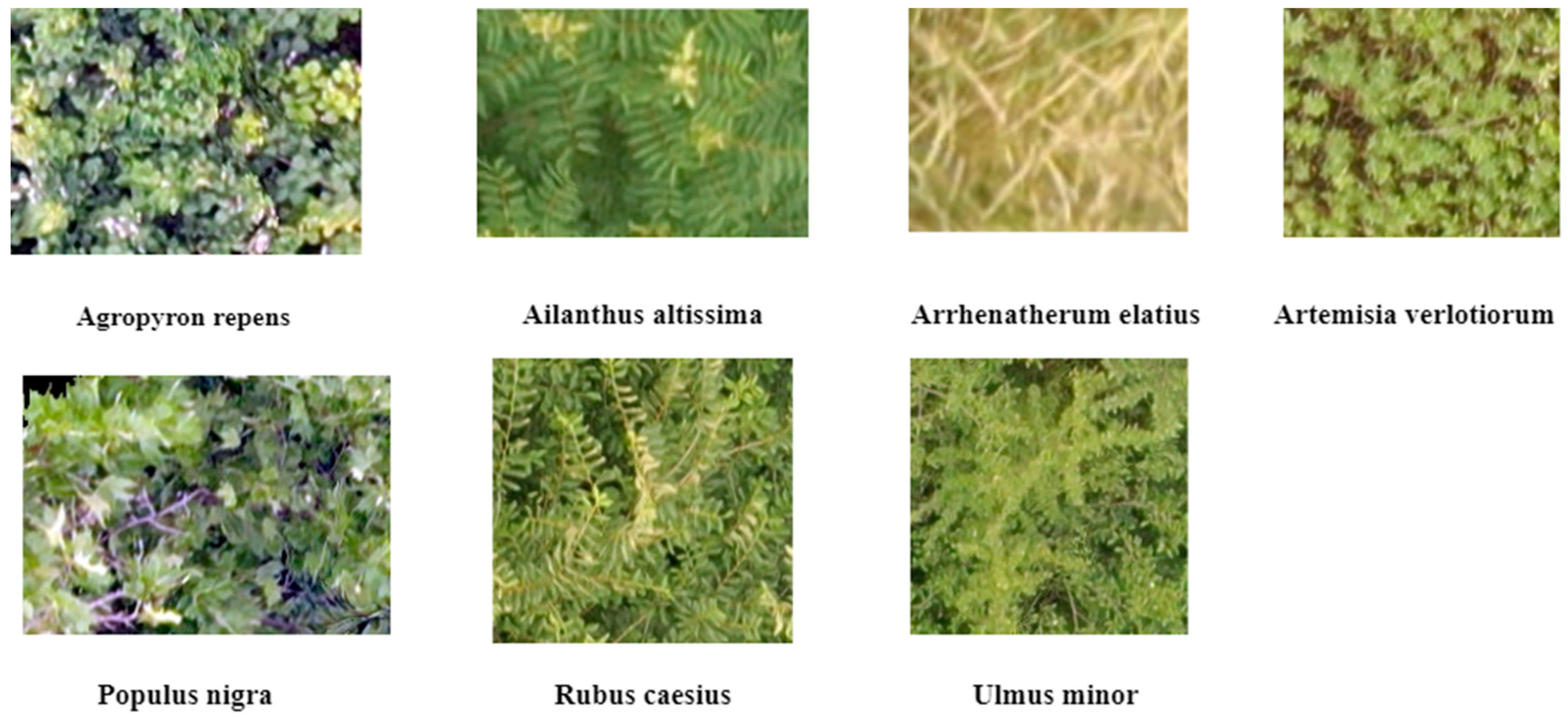
• We utilized plant mapping in an area with a diverse range of plant species and created a dedicated image dataset for the classification of seven distinct plant types. This approach stands in contrast to relying on publicly available datasets, which may encompass a wider range but could potentially introduce irrelevant or less accurate data into our analysis. Employing UAV datasets allows us greater control over data quality, ensuring that our findings are directly relevant to the precise areas under study.
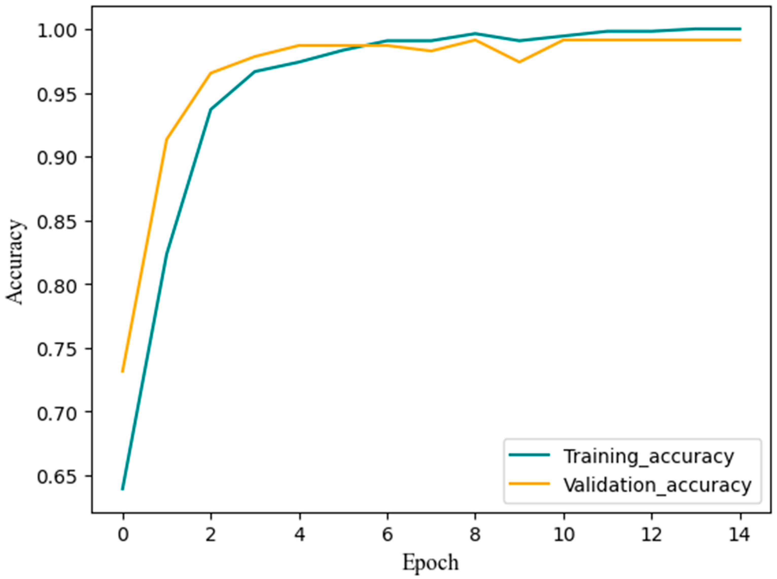
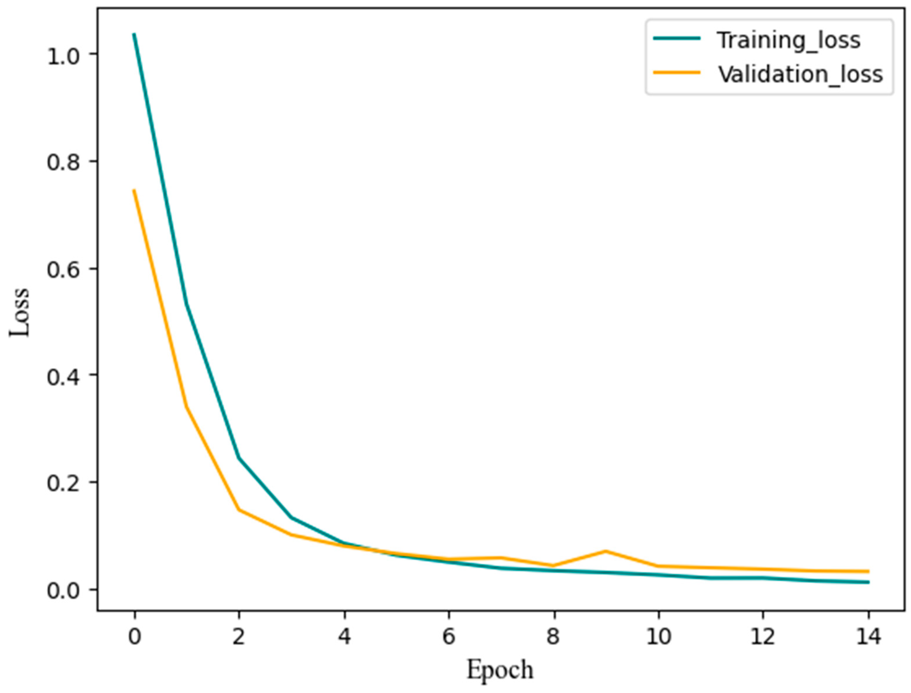
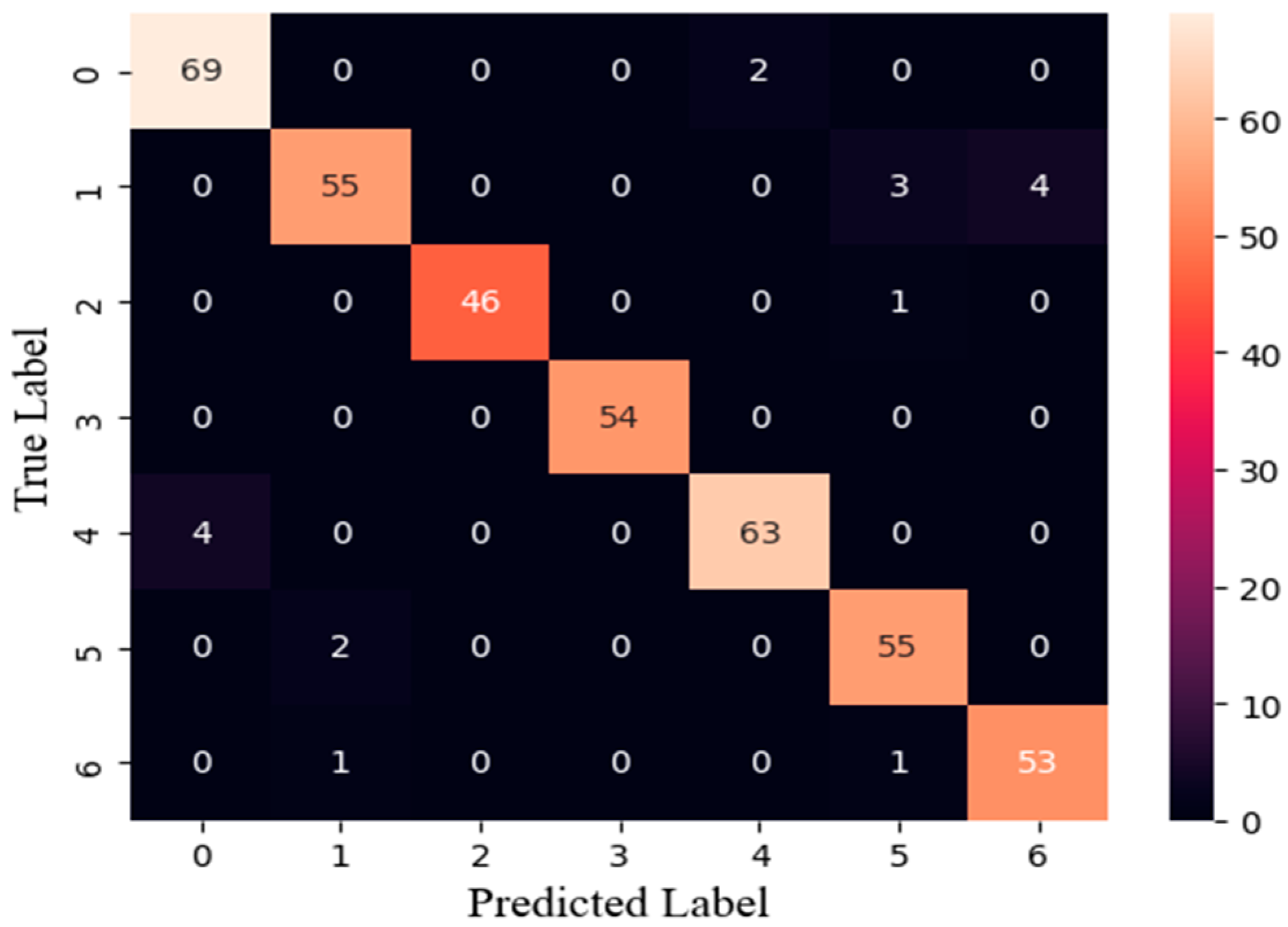
• The test results demonstrate that the fine-tuned pre-trained transfer learning model (EfficientNetV2) achieves a high classification accuracy of 99%. Such a high accuracy rate highlights the robustness and proficiency of the implemented approach in accurately identifying and distinguishing between various plant types.
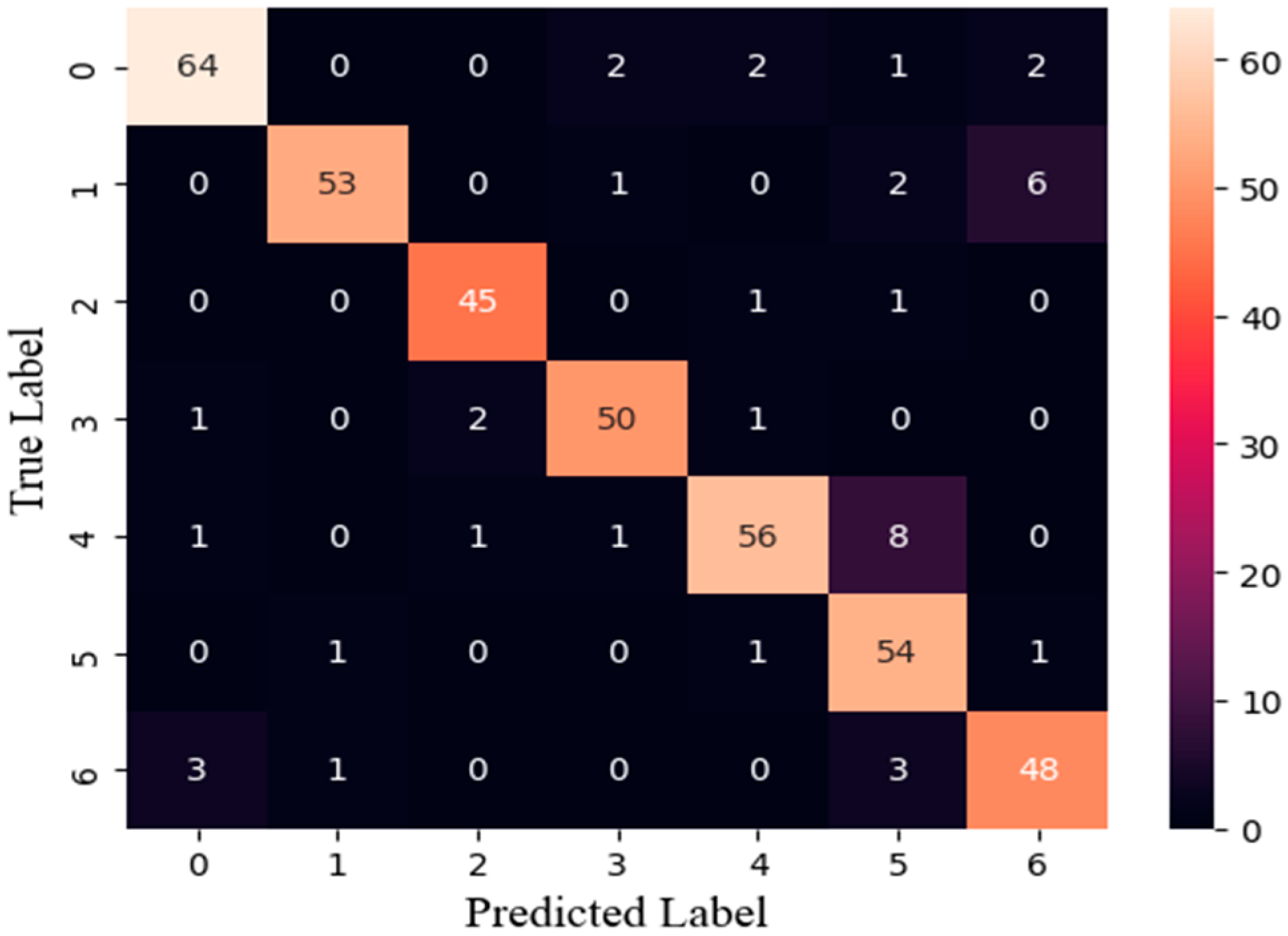
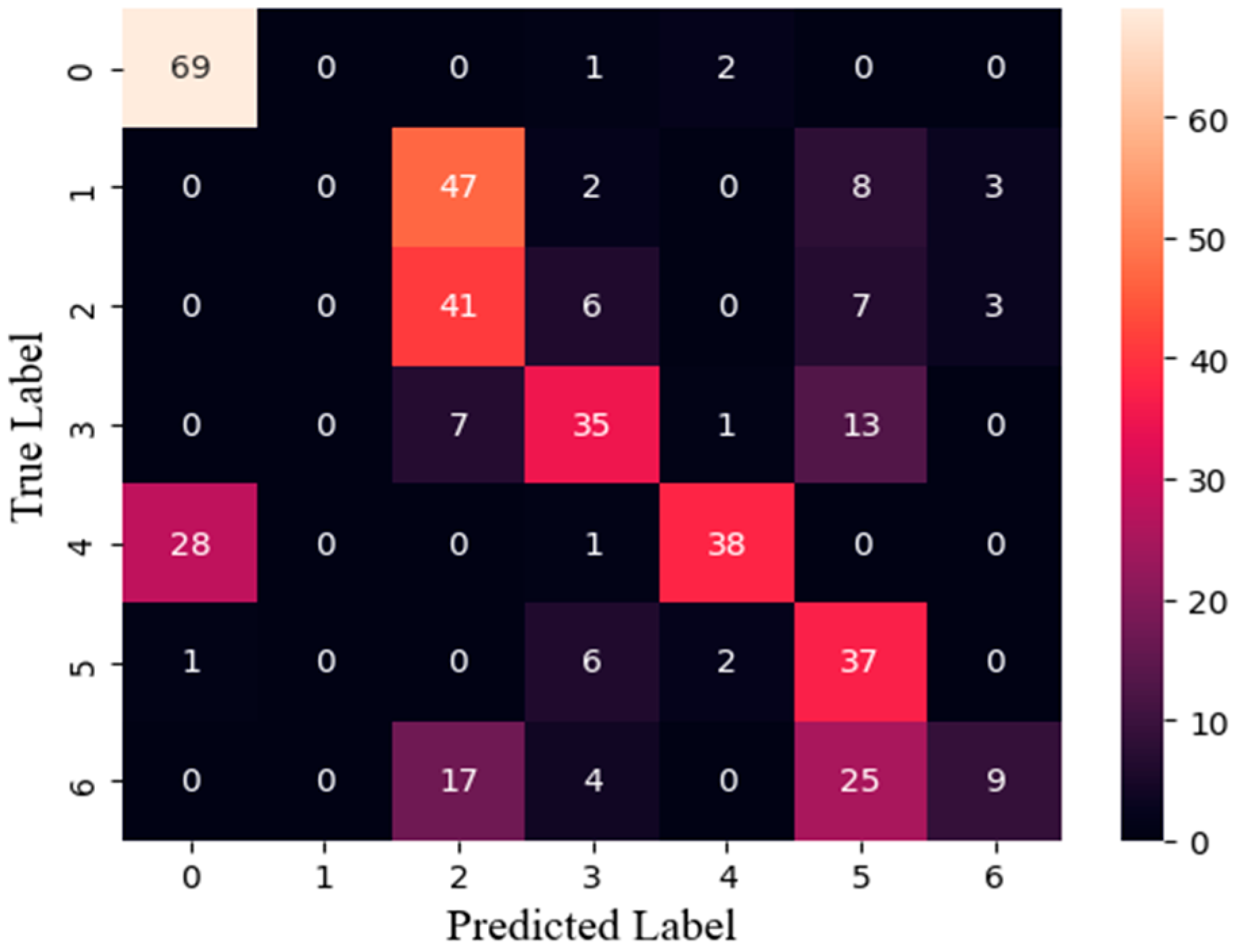
• A comparative study was also conducted, comparing the EfficientNetV2 model with other widely used transfer learning models, such as the ResNet50, Xception, DenseNet121, InceptionV3, and mobileNetV2, and providing a comprehensive understanding of their strengths and weaknesses.

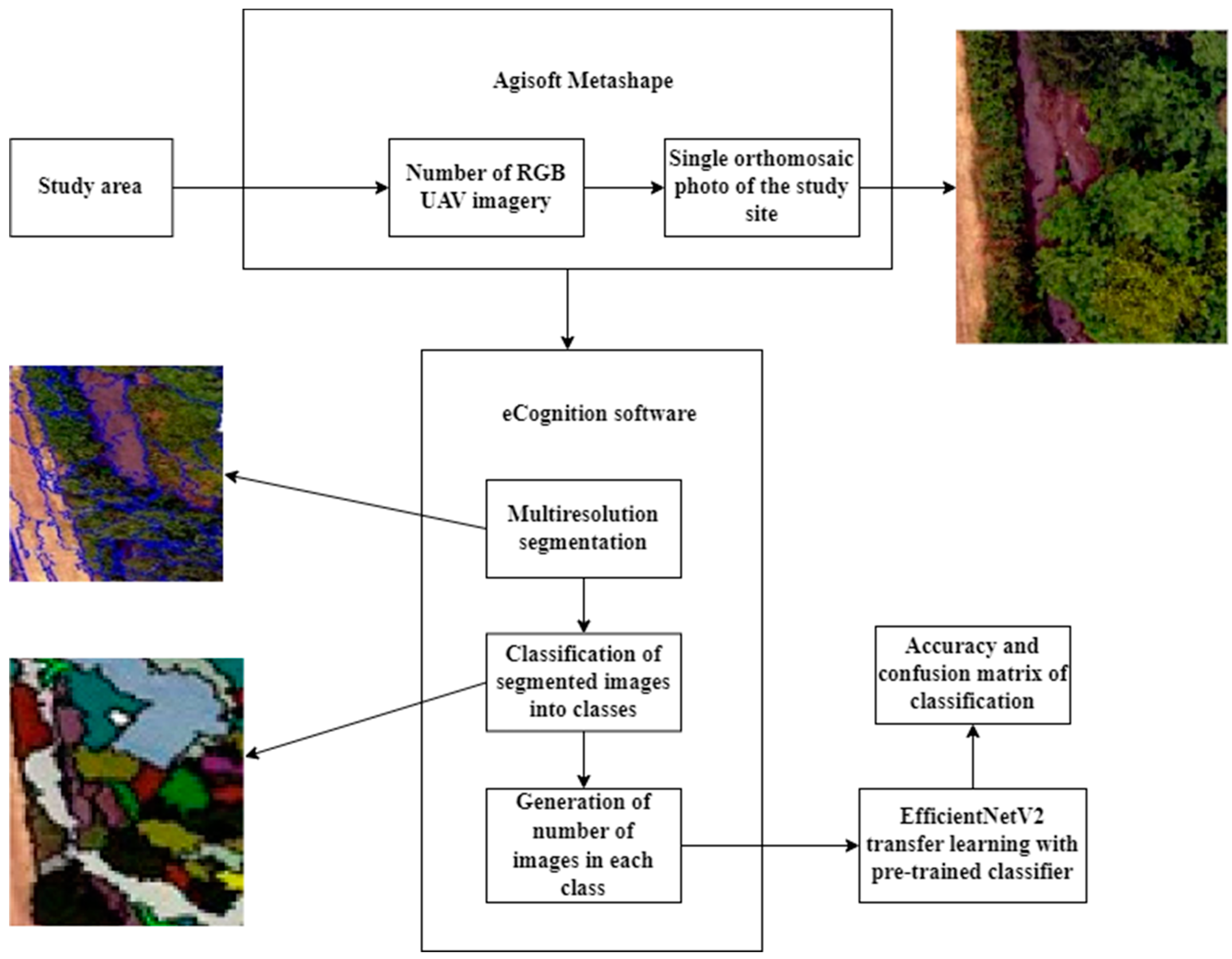
2. Materials and Methods

The method adopted in this research consists of the following five steps, as shown in Figure 1: study area (2.1); the acquisition of RGB images with a UAV platform (2.2); the pre-processing of the images, the labeling of the plant classes by a specialist using an eCognition software environment, and the mapping of plant classes using the KNN machine learning algorithm (2.3); the extraction of the seven classes of plant species through a mask using the ArcGIS software (2.4); and, finally, the classification performed using transfer learning (2.5).

2.1. Study Area

The study area encompasses an agricultural property within Parco Delle Cave in Brescia, Lombardy, Italy. Parco Delle Cave is a local park of supra-municipal interest, which extends over approximately 960 hectares, as shown in Figure 2. The specific study area covers one hectare and is located to the south-east of Brescia, a city in northern Italy.

The flight took place on 30 May 2022, using a Mavic 2 Pro UAV equipped with a Hasselblad L1D-20-megapixel camera. The drone operated automatically using Litchi, a software developed by the London-based VC Technology Ltd and designed for the DJI drone version 4.25.0 (released 4 July 2022). The Litchi software enabled us to carry out comprehensive photogrammetry missions using the drone. It set the flight altitude, determined the ground-level image resolution, and captured images covering the entire study area. The flight parameters were configured as follows: maintain a height of 30 meters above ground, incorporate four ground control points (GCPs), and integrate four targets for precise coordinates. A total of 319 images were captured in the designated area.

From the 319 drone images, we obtained an orthomosaic photo and a digital surface model (DSM) using the Agisoft Metashape V1.6.0 software. The software searched for “link points”—an obvious feature on each image—and for matches on every other image in the dataset. The total tie points for 319 images were 306,709 points.

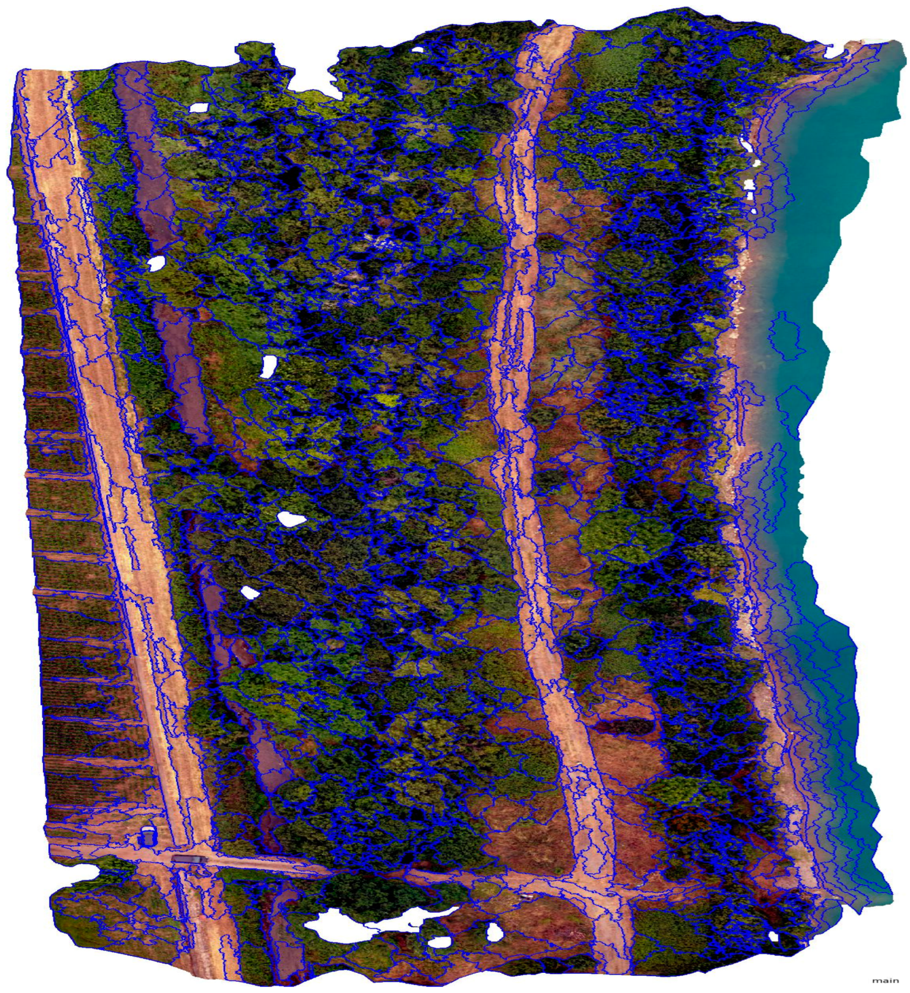
2.2. Object-Based Segmentation and Preparation of Supervised Data

The orthophoto was broken down into meaningful complete image-objects using segmentation techniques [27]. The orthophoto image and the DSM were used to segment the three canopies through the eCognition Developer v9.0.0 software (Trimble, Inc., Sunnyvale, CA, USA) using the “multi-resolution segmentation” tool. The multi-resolution segmentation algorithm [28] begins with a single pixel size and progressively merges segments into multiple iterations to form a unified larger unit.

During this segmentation, essential parameters such as scale, shape, and compactness were adjusted to achieve optimal results. These parameter values were fine-tuned until a satisfactory outcome was attained. More specifically, for this segmentation, the scale was set to 500; the compactness was set to 0.5; and the shape was set to 0.1. Following the multi-resolution segmentation, a subsequent step involved the spatial difference segmentation using the “Spatial Difference Segmentation” tool within the software. This process involves merging neighboring objects with spectral averages that are below a specified threshold. This merging process leads to the creation of the final segmented elements.

In particular, the threshold plays a central role in this merging process. In the case in question, a threshold of 20 was used to determine which spectral averages would be merged with the surrounding objects. This step helps to create a coherent and well-defined set of segmented elements, thereby improving the overall accuracy and interpretability of the segmentation results, as shown in Figure 3. The steps that follow were taken for the mapping of the plant species.

• Step 1. Segmentation and Feature Considerations:

After segmenting the image-objects using the eCognition software, localized pixel groups are selected. Most importantly, the features and spatial properties of these image-objects are considered in relation to each other. This segmentation approach ensures that meaningful groupings are formed, taking into account the feature relationships among adjacent objects.

• Step 2. Training Sample Selection:

These pixel groups, which represent different plant species, are strategically chosen to act as training samples for the supervised object-based classification algorithm. This process is devised to teach the software how to recognize different plant species on the basis of the patterns identified inside the pixel groups.

The plant species’ experts used color indicators that supported the training of samples for each plant species on the segmented image-object. The color indicator was prepared using a sheet of paper laid on the ground. We had put this indicator in the study area before the UAV flight and had made it visible on the orthophoto, as shown in Figure 4. The color indicator helps to determine the plant species for the training samples based on physically collected information about the type of plant species around the color indicator.

The preparation of these color indicators was a deliberate, hand-crafted process, meticulously executed on paper to ensure optimal visibility and accuracy. Before the UAV flight, these color indicators were strategically positioned within the study area. The intention behind this precise placement was to align them with specific areas of interest, where the presence of certain plant species was anticipated. This careful orchestration allowed the color indicators to serve as visual cues, imparting critical information about the types of plant species existing in the vicinity. This physical representation of the association of plant species with the color indicators serves as a tangible reference point, thus enhancing the reliability and accuracy of the subsequent training process.

• Step 3. Supervised Learning with the KNN Algorithm:

The classification process as such is achieved via supervised learning [29], a technique whereby the software learns from labeled training samples. More specifically, in mapping the plant classes, we used the “K-nearest neighbor (KNN)” eCognition software tool. The K-nearest neighbor (KNN) algorithm [30] is a machine learning method that assesses the proximity of pixels in the image against labeled training samples. By doing so, the presence of plant species is predetermined on the basis of attributes similar to those in labeled samples.

Fourteen classes were identified: twelve of these were plant species and one was lake water. One additional class was added manually to identify roads, cars, and plant species not included in our twelve classes of plant species. The merge region algorithm was used to merge all nearby image-objects of a class into one large object. Each class was subjected to this procedure.

The merge region algorithm was used to combine closely located image-objects of a specific class into a single, larger object. This procedure was carried out for each class separately. The “Merge Region” tool in the eCognition software was used in this process, which allowed us to merge each class individually. Two segmented image-objects were thus merged and class mapping was then completed: objects belonging to the same plant species class were merged together. Figure 5 illustrates the ultimate merged and mapped outcome of the orthophoto.

2.3. Tree Image Extraction with Ground Truth Label

After the classification mapping process using the eCognition software, as shown in Figure 5, the next step involved exporting each plant species class individually. This was achieved by using the image-object export feature in the eCognition software tool. This procedure was repeated for all the plant species classes. Subsequently, the extracted plant image-objects of each class were imported into the ArcGIS software, where they were further processed. The following steps were taken to extract the plant dataset:

• The plant class image was imported into the ArcGIS software.
• A polygon mask was prepared to define the size of the images in the dataset and represent them with a rectangular mask. This mask was used to shift and clip the images to a larger image.
• The “Extract by Mask” tool within ArcGIS was used to clip and generate an image dataset matching the size of the polygon mask, which was tailored to each specific plant species class.

This sequence of steps facilitated the creation of separate image datasets for each plant species, effectively contributing to the comprehensive dataset used for the subsequent analysis and classification tasks. A total of 782 images were generated across seven plant species classes.

A training dataset of seven classes was used from the twelve orthophoto-mapped plant species for classification according to a pre-trained model. We chose these seven plant species because, unlike the other classes, sufficient images were available for training. The visual sample images are provided in Figure 6.

Using the ‘Extract by Mask’ feature in ArcGIS, we extracted each plant image with a class label from the orthomosaic images. We manually eliminated incorrect photographs and it was agreed to assign correctly categorized images to the correct class. The incorrect images included the plant pieces that were difficult to identify or classify visually and those attributable to multiple classes.

2.4. Transfer Learning: EfficientNetV2

In order to overcome the lack of data and training time, the transfer learning technique is generally used in addition to data augmentation. Image augmentation is a technique used in computer vision and deep learning to increase the size of a dataset by creating modified versions of existing images. Rotation, shearing, flip vertical, and brightness functions were used to increase the total number of images from 782 to 1374.

Transfer learning is a machine learning technique that involves the use of the knowledge gained by training a model in one task and applying it to a different but related task [31,32]. In deep learning, transfer learning involves using a pre-trained neural network model, often trained on a large dataset, as a starting point for a new task. Rather than training a new model from scratch, transfer learning allows us to leverage the learned features and representations of a pre-trained model and fine-tune it for the new task.

The approach taken in this study involves leveraging a pre-trained transfer learning model known as EfficientNetV2, which is sourced from the TensorFlow hub. EfficientNetV2 is a cutting-edge convolutional neural network architecture that offers clear advantages in terms of both training speed and parameter efficiency [33]. Notably, these models are the result of a harmonious fusion of two key components: a neural architecture search that is tailored to training data, and a systematic scaling process. This integration is meticulously designed to achieve a synergistic optimization of both training speed and parameter efficiency, leading to a network architecture that is not only faster to train but also more effective in terms of using model parameters for improved performance. EfficientNetV2’s advanced design principles have made it stand out as an evolution in the field of convolutional neural networks by offering the potential to expedite training times while ensuring optimal utilization of computational resources.

The model is based on efficient ImageNet architectures that have been proven in transfer learning. The EfficientNetV2 models for feature extraction and image classification are trained on the ImageNet 1k (ILSVRC-2012-CLS) and ImageNet 21k (Full ImageNet, Fall 2011 release). The ImageNet ILSVRC2012 contains about 1.28 million training images and 50,000 validation images [34]. The model dataset contains 1000 object categories, which include both internal and leaf nodes from ImageNet but do not overlap with each other.

When classifying 1000 classes, most of the parameters in normal ImageNet models are concentrated at the top. However, the number of classes retrieved from our plant classification by masking seven classes was often much lower, which indicates that ImageNet models are likely over-parametrized. The most common way of transferring learning for deep learning is the following workflow:

• Take layers from a previously trained model.
• Freeze them, so as to avoid destroying any of the information they contain during future training rounds.
• Add some new, trainable layers on top of the frozen layers. They will learn to turn the old features into predictions on a new dataset.
• Train the new layers on the new dataset.

The EfficientNetV2 model was used in our case as follows: Firstly, the pre-trained EfficientNetV2 model was uploaded via its URL from the TensorFlow Hub (feature extractor model). The base layers of the model were frozen (trainable = false) to serve as feature extractors without modifying their weights. Then, the image classification model was constructed using a sequential model from the TensorFlow Kera’s. Starting with the EfficientNetV2 base model, additional layers were then added. To begin with, a dense layer was inserted with the number of plant species as a unit. Following this, a flattened layer was incorporated to transform the multi-dimensional feature maps into a 1D vector. Two more dense layers were appended to facilitate further classification. Ultimately, the final layer comprised output units (one for each plant class category) and used the softmax activation function for multi-class classification.

3. Results

3.1. Input Data Details

The total dataset consisted of 1374 plant images of size 384 × 384 pixels in seven classes extracted from the orthophoto. Of these, 70% were randomly selected for training purposes (i.e., 961 images), and the remaining 30% (i.e., 413 images) were kept as a test dataset, as shown in

Table 1. Overview of the total number of images, training images, and test images allocated for each plant species class.

Species	Total No. of Images	No. of Test Images	No. of Training Images
Agropyron repens	215	71	144
Ailanthus altissima	193	62	131
Arrhenatherum elatius	174	47	127
Artemisia verlotiorum	194	54	140
Populus nigra	208	67	141
Rubus caesius	182	57	125
Ulmus minor	208	55	153
Total	1374	413	961

. The training dataset was used for training the EfficientNetV2 for classification, while the test dataset was used for evaluating the effectiveness of the proposed classification method. To ensure clarity and consistency in our results, we implemented a consistent weight-balancing approach for both the training and testing sets across all pre-trained models using the Python Keras library, as outlined in Table 1.

3.2. Classification Model Evaluation

Four performance criteria were used: accuracy, recall, precision, and F1 score. To evaluate the test labels, the actual labels were compared with the predicted labels. The predicted results are summarized in Figure 7 in the form of a confusion matrix. Since our classes were balanced, accuracy was used to assess how good the predictions were. In addition to accuracy, other metrics such as precision, recall, and F1 score were also calculated (

Table 2. Performance measures for species classification results during final post-training. After averaging, the final trained network yields an overall accuracy of 0.99, an average precision of 0.99, an average recall of 0.99, and an average F1-score of 0.995.

Species	Precision	Recall	Accuracy	F1-Score
Agropyron repens	1.0	0.97	0.97	0.99
Ailanthus altissima	1.0	1.0	1.0	1.0
Arrhenatherum elatius	0.98	1.0	1.0	0.99
Artemisia verlotiorum	1.0	0.98	0.98	0.99
Populus nigra	0.97	1.0	1.0	0.99
Rubus caesius	1.0	1.0	1.0	1.0
Ulmus minor	1.0	1.0	1.0	1.0

).

3.3. Definition of the Terms

Let us first define the performance criteria used to evaluate the performance of the pre-trained model used.

Precision is the fraction of instances marked as positive that are indeed correct. Precision measures “how useful the results of our classifier are”.

$$P=\frac{T_p}{T_p+F_p}$$

(1)

Recall is the fraction of positive instances marked as positive. It measures “how complete the results are”, that is, what percentage of true positives are correctly identified.

$$R=\frac{T_p}{T_p+F_n}$$

(2)

F-1 score is the harmonic mean of precision and recall.

$$F1=2\frac{R·P}{R+P}$$

(3)

where $T_p$, $F_p$, and $F_n$ are true positive (number of predictions where the classifier correctly predicted positive class as positive), false positive (number of predictions where the classifier incorrectly predicts negative class as positive), and false negative (number of predictions where classifier predicts incorrectly negative class as positive), respectively.

We computed the standard deviation values for our seven classes in a classifier, taking into consideration the specific characteristics of the data and the issue at hand. The standard deviation values provided for each class and channel (R, G, B) indicate the extent of variability or spread in pixel values in each class and channel. In image classification, these values offer insights into the consistency or diversity of color distribution for each class across color channels.

The standard deviation values for each class are given below:

• Class 0: Standard Deviation values for channels R, G, B: [0.213517 0.2134958 0.1996962]
• Class 1: Standard Deviation values for channels R, G, B: [0.122984 0.11884958 0.08400311]
• Class 2: Standard Deviation values for channels R, G, B: [0.13345262 0.11413942 0.10716095]
• Class 3: Standard Deviation values for channels R, G, B: [0.12690945 0.13369219 0.10653751]
• Class 4: Standard Deviation values for channels R, G, B: [0.20748237 0.20688726 0.20193826]
• Class 5: Standard Deviation values for channels R, G, B: [0.15583675 0.15177113 0.12188773]
• Class 6: Standard Deviation values for channels R, G, B: [0.14056665 0.145093 0.09837905].

Interpreting the standard deviation values provided the following:

• Class 0: Pixel values in this class show a relatively high variability in the red and green channels compared to the blue channel.
• Class 1: Pixel values in this class show a low variability across all three color channels (R, G, B), indicating a more uniform color distribution.
• Class 2: Similarly to Class 1, pixel values in this class also show a relatively low variability across all three color channels.
• Class 3: Pixel values in this class show a moderate variability in the red and green channels, with a slightly high variability in the blue channel.
• Class 4: Pixel values in this class show a relatively high variability across all three color channels.
• Class 5: Pixel values in this class show a moderate variability in all three color channels.
• Class 6: Pixel values in this class show a moderate variability in the red and green channels, with a reduced variability in the blue channel.

Among the values provided, Class 4 stands out with relatively high standard deviation values, suggesting a greater diversity or spread of pixel values within that class and color channels. This indicates that the color distribution in Class 4 is more varied than in other classes.

Conversely, Class 1 shows relatively low standard deviation values across all three color channels (R, G, B), indicating a more consistent or uniform color distribution in that class.

3.4. Training Results

The training result of the proposed model is recorded and presented in the form of plots in Figure 8 and Figure 9 below. The orange curve stands for the validation and the blue curve stands for the training. The results of the curve show that the final validation accuracy rate is 99% and the final validation loss is 0.0128. This can be regarded as a positive sign for the classification results.

4. Discussion

The proposed article builds on the previous works of [25,26] and addresses a specific challenge in plant species classification. In [25], the authors suggested the use of a conjugate-dense CNN architecture (CD-CNN) with a novel activation function called SL-ReLU, while [26] proposed a pre-trained transfer learning model called Vit for accurate crop classification.

The studies conducted by [25,26] focused on gathering image datasets for image classification using UAV-collected RGB images. Datasets were collected for each labeled class in areas carefully selected in terms of homogeneity for each class. However, there was a significant research gap in terms of the acquisition and preparation of the datasets encompassing areas with diverse plant species.

To address this gap, we have developed a methodology for collecting an image dataset for plant image classification from heterogeneous plant areas using UAV-collected RGB images. Furthermore, previous studies have employed large image datasets to enhance classification accuracy. In contrast, we address this challenge by employing trained transfer learning, thereby significantly improving classification accuracy even when working with a limited number of datasets. It is important to note that performing image classification also requires more time for large datasets compared to small datasets.

The contribution of our study was to prove the classification ability of the pre-trained transfer learning model EfficientNetV2 for the UAV-collected RGB images of seven plant species in the relevant heterogenous area. The model classified plant species with a 99% accuracy race and a 0.98 F1 value. Another important task in this study was to increase the number of mapped plant species by using color indicators on the ground to distinguish plant canopies on the orthophotos.

We compared the pre-trained EfficientNetV2 with other widely used pre-trained transfer learning models in the field of image classification computer vision. The comparison study was performed on the same dataset, which is important to mention here. For the comparison, we used pre-trained transfer learning models such as the InceptionV3 [35], MobileNetV2 [36], Xception [37], DenseNet121 [38], and ResNet50 [39]; all of them had been pre-trained with the ImageNet dataset. The confusion matrices are shown in Figure 10, Figure 11, Figure 12, Figure 13 and Figure 14.

It can be noted that the ResNet50 technique performed the worst, with some misclassified images. This resulted in an accuracy of only 60.2%. The InceptionV3 (91.5%), DenseNet121 (95.3%), Xception (95.6%), and MobileNetV2 (96.6%) performed better than the ResNet50. However, the proposed EfficientNetV2 achieved the best classification accuracy for all the test classes (see

Table 3. Model comparison, each utilizing the same dataset employed in this study and processed on the same computer using the Python programming language. The table provides the final testing accuracy, precision, recall, and F1-Score values for each model.

Pre-trained Model	Pre-trained Dataset	Accuracy (%)	Precision	Recall	F1-Score
EfficientNetV2	ImageNet	99.2	0.992	0.993	0.993
MobileNetV2	ImageNet	96.6	0.967	0.964	0.965
Xception	ImageNet	0.956	0.955	0.958	0.954
DensNet121	ImageNet	0.953	0.951	0.953	0.951
InceptionV3	ImageNet	91.5	0.916	0.918	0.915
ResNet50	ImageNet	60.2	0.655	0.615	0.594

).

The supremacy of the EfficientNetV2 image classification model over the ResNet and other architectures in our classification task stems from its innovative design, which optimizes both depth and width parameters. EfficientNetV2 employs a composite scaling approach that systematically and concurrently increases the depth, width, and resolution of the network [33]. This approach enables the model to achieve an elevated accuracy while upholding computational efficiency.

Conversely, the ResNet primarily emphasizes increasing the network’s depth to enhance performance [39]. However, as the network grows deeper, issues like vanishing gradients and extended training times arise. The balanced scaling approach of the EfficientNetV2 ensures that the network does not become excessively deep or excessively wide, but rather strikes a harmonious balance that leverages both depth and width.

Moreover, the EfficientNetV2 employs a neural architecture search (NAS) to identify the optimal combination of depth, width, and resolution [40]. This results in a network that maximizes performance within a specified computational budget. Consequently, EfficientNetV2 achieves an increased accuracy while maintaining computational efficiency, rendering it well-suited to our plant image classification task, providing us with a superior accuracy compared to the other models.

In our work, we dealt with two main tasks. Firstly, we performed plant image classification using a pre-trained transfer learning model. The advantage of using a pre-trained model is that it can achieve good results even with a smaller training dataset compared to a non-pre-trained CNN model. With 1374 images from the training dataset for seven classes, our small dataset did not significantly impact the classification accuracy. However, it is worth noting that achieving a high accuracy in plant image classification with CNN models generally requires a large training dataset [25,26].

The use of transfer learning also reduces training time since the pre-trained model features serve as a starting point, and only a fraction of the total parameters needs to be trained. In the case of the EfficientNetV2, out of the 14 million total parameters, there are 4908 trainable parameters. This reduction in trainable parameters contributes to faster training.

Secondly, during the UAV flight, we employed a color indicator material to assist in the object-based classification for the plant mapping. This approach helps to identify individual plant species on the orthophoto. In mixed-cultivated agricultural areas, segmenting tree crowns using specific parameters can be challenging. Using a color indicator, we were able to alleviate some of the complexities associated with diversified areas. However, despite these efforts, misclassification of mapped objects still occurred, indicating areas for potential improvement.

The significance of this research study lies in its implications for plant identification and classification in areas with diverse and heterogeneous plant species, supporting biodiversity studies. Using UAVs and RGB images you can capture specific study areas or regions of interest, thereby reducing data volume and improving analysis efficiency. When employing transfer learning techniques, knowledge from larger datasets can be transferred to improve the performance of models trained on smaller datasets, thus enabling more cost-effective and efficient plant species classification.

In order to enhance the effectiveness of plant classification and mapping, we recommend that future researchers prioritize collecting UAV images for specific heterogeneous areas in different seasons. This approach will help to understand plant image characteristics across different conditions and test the classification model’s performance under diverse circumstances. By integrating deep learning into the conventional mapping approach, researchers can further improve plant classification and mapping accuracy.

5. Conclusions

This article describes a method for the accurate identification and classification of plant species in heterogeneous areas using UAV-collected RGB images, plant mapping techniques, and transfer learning. The study emphasizes challenges in precise species identification within diverse environments, focusing on dataset acquisition, preparation and model selection. Our approach combines object-based supervised machine learning with EfficientNetV2 transfer learning. In this study, we used several commercial software tools, including eCognition and ArcGIS. While these tools provide free versions, it is important to recognize their potential limitations. We employed supervised classification and the KNN algorithm via the eCognition software for plant mapping, collecting a dataset of seven plant species using the “Extract by Mask” tool within ArcGIS. Among the transfer learning models (ResNet50, InceptionV3, Xception, DenseNet121, and EfficientNetV2), EfficientNetV2 demonstrated an exceptional performance with 99% accuracy. This research enhances plant species identification and mapping techniques by providing a valuable tool for ecological and agricultural studies. As we progress, the integration of advanced machine learning and UAV technology will remain crucial for comprehending and conserving agroecosystem biodiversity. This study’s methodology is suitable for private and public companies seeking to study natural and semi-natural areas in support of biodiversity and territorial planning efforts. Researchers intending to employ these tools should consider the potential costs and constraints associated with commercial software. Further research should explore the method’s applicability across diverse geographical regions and account for additional factors influencing identification accuracy, thereby enhancing its robustness and generalizability.

References

1. Cope, J.S.; Corney, D.; Clark, J.Y.; Remagnino, P.; Wilkin, P. Plant species identification using digital morphometrics: A review. Expert Syst. Appl. 2012, 39, 7562–7573. [Google Scholar] [CrossRef]
2. Grinblat, G.L.; Uzal, L.C.; Larese, M.G.; Granitto, P.M. Deep learning for plant identification using vein morphological patterns. Comput. Electron. Agric. 2016, 127, 418–424. [Google Scholar] [CrossRef]
3. Dyrmann, M.; Karstoft, H.; Midtiby, H.S. Plant species classification using deep convolutional neural network. Biosyst. Eng. 2016, 151, 72–80. [Google Scholar] [CrossRef]
4. Kaya, A.; Keceli, A.S.; Catal, C.; Yalic, H.Y.; Temucin, H.; Tekinerdogan, B. Analysis of transfer learning for deep neural network based plant classification models. Comput. Electron. Agric. 2019, 158, 20–29. [Google Scholar] [CrossRef]
5. Barbedo, J.G.A. Impact of dataset size and variety on the effectiveness of deep learning and transfer learning for plant disease classification. Comput. Electron. Agric. 2018, 153, 46–53. [Google Scholar] [CrossRef]
6. Chen, F.; Tsou, J.Y. Assessing the effects of convolutional neural network architectural factors on model performance for remote sensing image classification: An in-depth investigation. Int. J. Appl. Earth Obs. Geoinf. 2022, 112, 102865. [Google Scholar] [CrossRef]
7. Weiss, K.; Khoshgoftaar, T.M.; Wang, D.D. A survey of transfer learning. J. Big Data 2016, 3, 1345–1459. [Google Scholar] [CrossRef]
8. Chen, J.; Chen, J.; Zhang, D.; Sun, Y.; Nanehkaran, Y. Using deep transfer learning for image-based plant disease identification. Comput. Electron. Agric. 2020, 173, 105393. [Google Scholar] [CrossRef]
9. Ahmadibeni, A.; Jones, B.; Shirkhodaie, A. Transfer learning from simulated SAR imagery using multi-output convolutional neural networks. In Applications of Machine Learning 2020, Presented at the SPIE Optical Engineering + Applications, Online, CA, USA, 24 August–4 September 2020; Zelinski, M.E., Taha, T.M., Howe, J., Awwal, A.A., Iftekharuddin, K.M., Eds.; SPIE: Philadelphia, PA, USA, 2020; p. 30. [Google Scholar] [CrossRef]
10. Fyleris, T.; Kriščiūnas, A.; Gružauskas, V.; Čalnerytė, D.; Barauskas, R. Urban Change Detection from Aerial Images Using Convolutional Neural Networks and Transfer Learning. ISPRS Int. J. Geo-Inf. 2022, 11, 246. [Google Scholar] [CrossRef]
11. Liu, J.; Chen, K.; Xu, G.; Sun, X.; Yan, M.; Diao, W.; Han, H. Convolutional Neural Network-Based Transfer Learning for Optical Aerial Images Change Detection. IEEE Geosci. Remote Sens. Lett. 2020, 17, 127–131. [Google Scholar] [CrossRef]
12. Rostami, M.; Kolouri, S.; Eaton, E.; Kim, K. Deep Transfer Learning for Few-Shot SAR Image Classification. Remote Sens. 2019, 11, 1374. [Google Scholar] [CrossRef]
13. Bin Tufail, A.; Ullah, I.; Khan, R.; Ali, L.; Yousaf, A.; Rehman, A.U.; Alhakami, W.; Hamam, H.; Cheikhrouhou, O.; Ma, Y.-K. Recognition of Ziziphus lotus through Aerial Imaging and Deep Transfer Learning Approach. Mob. Inf. Syst. 2021, 2021, 4310321. [Google Scholar] [CrossRef]
14. Lu, Y.; Young, S. A survey of public datasets for computer vision tasks in precision agriculture. Comput. Electron. Agric. 2020, 178, 105760. [Google Scholar] [CrossRef]
15. Hunt, E.R., Jr.; Daughtry, C.S.T. What good are unmanned aircraft systems for agricultural remote sensing and precision agriculture? Int. J. Remote Sens. 2018, 39, 5345–5376. [Google Scholar] [CrossRef]
16. Bouguettaya, A.; Zarzour, H.; Kechida, A.; Taberkit, A.M. Deep learning techniques to classify agricultural crops through UAV imagery: A review. Neural Comput. Appl. 2022, 34, 9511–9536. [Google Scholar] [CrossRef]
17. Kentsch, S.; Lopez Caceres, M.L.; Serrano, D.; Roure, F.; Diez, Y. Computer Vision and Deep Learning Techniques for the Analysis of Drone-Acquired Forest Images, a Transfer Learning Study. Remote Sens. 2020, 12, 1287. [Google Scholar] [CrossRef]
18. Dash, J.P.; Watt, M.S.; Pearse, G.D.; Heaphy, M.; Dungey, H.S. Assessing very high resolution UAV imagery for monitoring forest health during a simulated disease outbreak. ISPRS J. Photogramm. Remote Sens. 2017, 131, 1–14. [Google Scholar] [CrossRef]
19. Torresan, C.; Berton, A.; Carotenuto, F.; Di Gennaro, S.F.; Gioli, B.; Matese, A.; Miglietta, F.; Vagnoli, C.; Zaldei, A.; Wallace, L. Forestry applications of UAVs in Europe: A review. Int. J. Remote Sens. 2017, 38, 2427–2447. [Google Scholar] [CrossRef]
20. Xu, W.; Luo, W.; Zhang, C.; Zhao, X.; von Gadow, K.; Zhang, Z. Biodiversity-ecosystem functioning relationships of overstorey versus understorey trees in an old-growth temperate forest. Ann. For. Sci. 2019, 76, 64. [Google Scholar] [CrossRef]
21. Nasiri, V.; Darvishsefat, A.A.; Arefi, H.; Griess, V.C.; Sadeghi, S.M.M.; Borz, S.A. Modeling Forest Canopy Cover: A Synergistic Use of Sentinel-2, Aerial Photogrammetry Data, and Machine Learning. Remote Sens. 2022, 14, 1453. [Google Scholar] [CrossRef]
22. Onishi, M.; Ise, T. Explainable identification and mapping of trees using UAV RGB image and deep learning. Sci. Rep. 2021, 11, 903. [Google Scholar] [CrossRef] [PubMed]
23. Akcay, O.; Avsar, E.O.; Inalpulat, M.; Genc, L.; Cam, A. Assessment of Segmentation Parameters for Object-Based Land Cover Classification Using Color-Infrared Imagery. ISPRS Int. J. Geo-Inf. 2018, 7, 424. [Google Scholar] [CrossRef]
24. Gašparović, M.; Zrinjski, M.; Barković, Đ.; Radočaj, D. An automatic method for weed mapping in oat fields based on UAV imagery. Comput. Electron. Agric. 2020, 173, 105385. [Google Scholar] [CrossRef]
25. Pandey, A.; Jain, K. An intelligent system for crop identification and classification from UAV images using conjugated dense convolutional neural network. Comput. Electron. Agric. 2022, 192, 106543. [Google Scholar] [CrossRef]
26. Reedha, R.; Dericquebourg, E.; Canals, R.; Hafiane, A. Transformer Neural Network for Weed and Crop Classification of High Resolution UAV Images. Remote Sens. 2022, 14, 592. [Google Scholar] [CrossRef]
27. Blaschke, T. Object based image analysis for remote sensing. ISPRS J. Photogramm. Remote Sens. 2010, 65, 2–16. [Google Scholar] [CrossRef]
28. Benz, U.C.; Hofmann, P.; Willhauck, G.; Lingenfelder, I.; Heynen, M. Multi-resolution, object-oriented fuzzy analysis of remote sensing data for GIS-ready information. ISPRS J. Photogramm. Remote Sens. 2004, 58, 239–258. [Google Scholar] [CrossRef]
29. Ma, L.; Li, M.; Ma, X.; Cheng, L.; Du, P.; Liu, Y. A review of supervised object-based land-cover image classification. ISPRS J. Photogramm. Remote Sens. 2017, 130, 277–293. [Google Scholar] [CrossRef]
30. Deng, Z.; Zhu, X.; Cheng, D.; Zong, M.; Zhang, S. Efficient kNN classification algorithm for big data. Neurocomputing 2016, 195, 143–148. [Google Scholar] [CrossRef]
31. Mehmood, T.; Gerevini, A.; Lavelli, A.; Serina, I. Leveraging Multi-task Learning for Biomedical Named Entity Recognition. In AI*IA 2019—Advances in Artificial Intelligence; Alviano, M., Greco, G., Scarcello, F., Eds.; Lecture Notes in Computer Science; Springer International Publishing: Cham, Switzerland, 2019; pp. 431–444. [Google Scholar]
32. Mehmood, T.; Gerevini, A.E.; Lavelli, A.; Serina, I. Combining Multi-task Learning with Transfer Learning for Biomedical Named Entity Recognition. Procedia Comput. Sci. 2020, 176, 848–857. [Google Scholar] [CrossRef]
33. Tan, M.; Le, Q.V. EfficientNetV2: Smaller Models and Faster Training. arXiv 2021, arXiv:2104.00298. [Google Scholar] [CrossRef]
34. Russakovsky, O.; Deng, J.; Su, H.; Krause, J.; Satheesh, S.; Ma, S.; Huang, Z.; Karpathy, A.; Khosla, A.; Bernstein, M.; et al. ImageNet Large Scale Visual Recognition Challenge. Int. J. Comput. Vis. 2015, 115, 211–252. [Google Scholar] [CrossRef]
35. Szegedy, C.; Vanhoucke, V.; Ioffe, S.; Shlens, J.; Wojna, Z. Rethinking the Inception Architecture for Computer Vision. In Proceedings of the IEEE Conference on Computer Vision and Pattern Recognition, Las Vegas, NV, USA, 27 June–28 July 2016; pp. 2818–2826. Available online: https://www.cv-foundation.org/openaccess/content_cvpr_2016/html/Szegedy_Rethinking_the_Inception_CVPR_2016_paper.html (accessed on 22 April 2023).
36. Sandler, M.; Howard, A.; Zhu, M.; Zhmoginov, A.; Chen, L.-C. MobileNetV2: Inverted Residuals and Linear Bottlenecks. arXiv 2019, arXiv:1801.04381. [Google Scholar] [CrossRef]
37. Chollet, F. Xception: Deep Learning with Depthwise Separable Convolutions. arXiv 2017, arXiv:1610.02357. [Google Scholar] [CrossRef]
38. Huang, G.; Liu, Z.; van der Maaten, L.; Weinberger, K.Q. Densely Connected Convolutional Networks. arXiv 2018, arXiv:1608.06993. [Google Scholar] [CrossRef]
39. He, K.; Zhang, X.; Ren, S.; Sun, J. Deep Residual Learning for Image Recognition. In Proceedings of the IEEE Conference on Computer Vision and Pattern Recognition, Las Vegas, NV, USA, 27 June–28 July 2016; pp. 770–778. Available online: https://openaccess.thecvf.com/content_cvpr_2016/html/He_Deep_Residual_Learning_CVPR_2016_paper.html (accessed on 22 April 2023).
40. Tan, M.; Le, Q.V. EfficientNet: Rethinking Model Scaling for Convolutional Neural Networks. arXiv 2020, arXiv:1905.11946. [Google Scholar] [CrossRef]
Figure 1. Illustration of the proposed method for plant species identification and classification.
Drones 07 00599 g001
Figure 2. Above left: Parco delle Cave map in Brescia, Italy. Above right: close-up of the study area.
Drones 07 00599 g002
Figure 3. Representation of the segmented orthophoto acquired using the multi-resolution segmentation technique with the eCognition software. The segmented image-objects are identified by the blue line, which gives a clear view of the segmentation process.
Drones 07 00599 g003
Figure 4. The entire area represents a single captured image taken by the drone from a height of 30 meters. The yellow paper serves as a color indicator. The color indicator helps to determine the plant species for the training samples based on physically collected information on the type of plant species near the color indicator.
Drones 07 00599 g004
Figure 5. Ground truth plant mapping using the eCognition software, with distinct plant species classes color-coded according to the provided legend.
Drones 07 00599 g005
Figure 6. Images taken from each labeled class. These images were meticulously generated using the ArcGIS software and the ‘Extract by Mask’ tool with the rectangular polygon. With this process specific plant species could be isolated from larger images, thereby contributing to the creation of a comprehensive dataset for further analysis and classification.
Drones 07 00599 g006
Figure 7. Confusion matrix result for plant species classification with the EfficientNetV2 model. Numbers in the matrix identify the samples classified in each class, and the color helps to identify where more samples are classified. The label for each class: zero for Agropyron repens, one for Ailanthus altissima, two for Arrhenatherum elatius, three for Artemisia verlotiorum, four for Populus nigra, five for Rubus caesius, and six for Ulmus minor.
Drones 07 00599 g007
Figure 8. The curves in the graph indicate the training and validation accuracies achieved using the pre-trained EfficientNetV2 model on a dataset consisting of RGB UAV-collected images for seven labeled classes of plant images. The Y-axis represents accuracy values, and the X-axis represents the number of epochs.
Drones 07 00599 g008
Figure 9. Training and validation losses achieved by using the EfficientNetV2 pre-trained model on a dataset comprising RGB UAV-collected images for seven labeled classes of plant images. The Y-axis represents the loss values, and the X-axis corresponds to the number of epochs.
Drones 07 00599 g009
Figure 10. Confusion matrix for the InceptionV3 and the label for each class: zero for Agropyron repens, one for Ailanthus altissima, two for Arrhenatherum elatius, three for Artemisia verlotiorum, four for Populus nigra, five for Rubus caesius, and six for Ulmus minor.
Drones 07 00599 g010
Figure 11. Confusion matrix for the ResNet50 and the label for each class: zero for Agropyron repens, one for Ailanthus altissima, two for Arrhenatherum elatius, three for Artemisia verlotiorum, four for Populus nigra, five for Rubus caesius, and six for Ulmus minor.
Drones 07 00599 g011
Figure 12. Confusion matrix for the DensNet121 and the label for each class: zero for Agropyron repens, one for Ailanthus altissima, two for Arrhenatherum elatius, three for Artemisia verlotiorum, four for Populus nigra, five for Rubus caesius, and six for Ulmus minor.
Drones 07 00599 g012
Figure 13. Confusion matrix for the Xception and the label for each class: zero for Agropyron repens, one for Ailanthus altissima, two for Arrhenatherum elatius, three for Artemisia verlotiorum, four for Populus nigra, five for Rubus caesius, and six for Ulmus minor.
Drones 07 00599 g013
Figure 14. Confusion matrix for the MobileNetV2 and the label for each class: zero for Agropyron repens, one for Ailanthus altissima, two for Arrhenatherum elatius, three for Artemisia verlotiorum, four for Populus nigra, five for Rubus caesius, and six for Ulmus minor.
Drones 07 00599 g014