1. Introduction
Very recently, the use of small unmanned aerial vehicles (UAVs) has significantly increased. These tiny vehicles, also known as drones, are being used more and more frequently, particularly for a variety of tasks, including the production of toys for kids, entertainment, photography, video monitoring in remote locations, agronomy, military intelligence, delivery, and transportation. The purpose of their widespread use in the postal service and agriculture is the automation of processes in order to replace the workforce. Due to the many recreational uses of these UAVs, illegal activities with them have also increased or at least become more visible than before. These vehicles are said to have been used in smuggling drugs across international borders, violating airport security and local laws. The main reason for their frequent use among people is the expansion of their technical capabilities, i.e., an increase in flight duration, the possibility of flexible video filming from different heights and angles, and the possibility of unhindered entry into different areas. Furthermore, over the past decade, the mass production of unmanned aerial vehicles (UAVs) at affordable prices has led to the problem of the constant use of these devices for various dubious and recreational purposes. The careless or harmful use of these vehicles can endanger people, their lives and protected institutions, and the border areas of countries. These reasons take into account the fact that UAVs are becoming more and more dangerous. Recently, there have been several incidents with drones [
1,
2,
3,
4,
5,
6,
7,
8,
9]. In particular, in 2015, an intoxicated government official in front of the White House lawn in the United States provoked a drone crash, in 2017 a plane landing in Canada had a minor accident with a drone, and a suspicious drone flew over Gatwick Airport in London in 2018, causing thousands of passengers to cancel flights [
3]. There are many cases of damage caused, especially by improper management. Likewise, an Unmanned Aerial Vehicle (UAV) crash occurred in the city of Asir on the border with Saudi Arabia [
10]. Another drone crash happened in China: a dozen of the 200 drones took to the skies during a light show in Zhengzhou. In this case of UAV crashes, just 2.5 min after their glorious ascent, the drones began to fall back to the ground, crashing into trees, cars, and everything else as they fell. Some participants of this show ran to hide from unmanned drones [
11]. In general, the reasons for the impossibility of the sustainable use of these vehicles are discussed in more detail in [
3,
5]. Thus, the high frequency of unauthorized drone flights requires the development of reliable real-time drone detection systems for protected areas. Therefore, the detection systems for the unauthorized use of UAVs are becoming more and more significant, especially in the buildings of institutions such as schools, kindergartens, hospitals, universities, administrations, ministries, border areas of the country, protected areas where military bases are located, reservoirs that protect large cities from snowmelt, and agricultural locations. For these reasons, there has been a growing demand for research into security measures based on drone detection systems to prevent the spread of unauthorized drones in restricted and protected strategic areas.
The potential risks with UAVs are more related to factors such as poor control or human error, as well as malicious use, especially when they have an additional load while flying in crowded areas. In these regards, the problem of automatic audio-based UAV classification and detection systems has attracted particular interest from the research community due to their ability to detect loaded and unloaded UAV states in certain areas of interest [
1,
3]. The recognition of the UAV’s load by acoustic sensors is more effective than other methods such as radar, camera, and radio frequency methods [
5,
6,
7]; thus, this work aims to investigate the acoustic sensor method for the UAV detection problem.
In general, taking into account the mentioned UAV incidents, UAV threats can be divided into two main categories. Unmanned aerial vehicles used for amateur purposes, in most cases, will not carry an extra load during their flight, so they fall into the category of less threatening. At the same time, UAVs used in terrorist and malicious attacks often carry an additional load. Therefore, UAVs of a similar category or poorly controlled loaded UAVs belong to the group of the most threatening objects. In the case where the UAV poses a real public threat, resources can be directed to the real threat and not to less or more threatening phenomena. In order to ensure simultaneous detection of both threatening UAVs, this research work proposes a new approach with the task of classifying loaded and unloaded UAVs based on acoustic signals in the presence of different UAV models and different payload masses. The purpose behind identifying UAVs by acoustic signatures lies in the fact that if the UAV has an additional load during the flight, the supplemented mass makes changes in the recognition system database, and likewise, the acoustic signature will change. The signature of the UAV without load differs from the signature of the UAV with a one-kilogram Cemtex stick or other explosive material attached to the bottom of the vessel [
1]. In order to recognize the differences between these UAV acoustic signatures, our research paper proposes a new recognition system structure based on the frequency features and Recurrent neural network cells. The motivation for this study was the lack of a drone recognition system that could take into account the reliable recognition of different UAV models with different payload masses in real-time. In addition, by analyzing related works in sound detection systems [
12], RNN has chosen robust computational neurons for recognizing different audio signal content, including UAV audio signals too. In parallel, the CNN algorithm, which in the previous statements is claimed to be a successful and reliable system, was experimented with a similar density as RNN. The new approach of our methodology is based on the study of a few models of Recurrent Neural Networks such as Simple RNN, LSTM, Bidirectional LSTM (BiLSTM), and Gated Recurrent Units (GRU) on the basis of Mel-spectrograms using the Kapre Method with fixed hyperparameters as in Table 3 and Figure 5. In addition, studies of drone-load identification tasks in [
1,
3] are based solely on one type of drone, in particular, the DJI Phantom 2. Consequently, our approach performs an additional study of the sounds of several drone models, as well as their real-time detection during every second of observation time for protected areas.
Generally, Simple RNN, Long Shot-Term Memory Network (LSTM), Bidirectional Long Short-Term Memory Network (BiLSTM), and Gated Recurrent Network (GRU) Neural Cells are Recurrent Neural Network (RNN) architectures designed for sequencing problems. Another advantage of these networks is that they are also able to learn the time dependence of given data. That is, the network shows one observation in a sequence and can figure out which of the observations it has seen before are relevant and how important they are for predictions [
12]. Therefore, our research work was aimed at experimentally studying these SimpleRNN, LSTM, BiLSTM, and GRU for UAV sound signals. To determine the cell robustness of RNN neurons, their results were compared with CNN models to see how they solve UAV sound classification problems. Furthermore, RNN models were actively studied in this work for the first time in the problem of classifying UAV acoustic signatures by assessing their payload. In accordance with the purpose of the work, research and experimental stages were considered based on the following tasks: (1) creation of a database of UAV sounds of different masses with different UAV models; (2) conducting extensive experimental studies for RNN cell types and developing structures for these neurons with additional hyperparameters; (3) the study of its recognition based on a system of previous studies in this direction with a small number of CNN layers and comparing the result with the results of RNN; (4) identifying and evaluating an effective system based on the results obtained.
This research work has five key sections that are all focused on research. The introductory section discusses the drone recognition system in general and the relevance of drone sound recognition in it. The second section of similar works examines the successes and drawbacks of prior research in this area. A theoretical foundation for the suggested RNN systems was attempted in the third section. The process, including data collection and frequency feature extraction, is covered in the fourth part. The results were examined, and an attempt was made to assess an efficient system in the fifth section.
2. Related Studies
Recognition of the UAVs according to their acoustic signals aroused extraordinary interest among researchers since they are able to solve scientific problems, such as UAV detection in conditions of poor visibility or identification of UAVs when it carries an additional burden. General studies of UAV detection systems have been discussed in detail in [
3,
5]. This section briefly discusses the survey of sound-based UAV detection and localization tasks. Successful detection or localization of these UAVs has been achieved primarily through machine learning, including deep learning techniques. Accordingly, this section discussed the classification of research works based on machine learning, deep learning, and other methods.
Machine learning methods in UAV sound recognition. Nijim et al. [
13] studied a drone detection system from its acoustic signatures using a Hidden Markov Model on DJI Phantom 3 and the FPV 250 drones dataset. The authors of [
14] processed the data of audio files into time and frequency parameters using the traditional ML method, SVM. They performed the task of binary classification, i.e., the presence or absence of a drone, as well as UAV sound spectrum images trained with a k-nearest neighbor (KNN) classifier (61%) and correlation (83%) methods to detect DJI Phantom 1 and 2 in [
15]. The problem of classification of drones into many types in the context of clustering of environmental noise and other types of noise (car, bird, rain) was carried out in the [
16] using the HMM method on the basis of 24 and 36 using MFCC features. The authors of [
17] studied the classification of flight sounds of DJI Spark, Quadcopter AR Drone 2.0, and Parrot Mambo drones using the random forest method. The SVM method classified the features using MFCC and LPCC coefficients in [
18]. The real-time detection of drone sounds was performed by two methods: PIL (Plotted Image Machine Learning) and KNN (K Nearest Neighbors) classification in [
15]. Reference [
19] integrated sensors such as a camera and a microphone; video frames were classified by HOG parameters, and audio frames were classified by SVM through MFCC parameters.
Machine learning and deep learning methods in UAV sound recognition. Jeon et al. [
20] investigated the detection of the drone existence in the range of 150 m with the Gaussian Mixture Model (68%), CNN (80%), and RNN (58%). Yang B. et al. proposed classifying the MFCCs and the STFT features with SVM and CNN models in [
21].
Deep learning methods in UAV sound recognition. In the works [
4,
22], CNN network models performed various classification tasks, such as the absence of drones in the region, the presence of drones, and the presence of two drones, and references [
1,
2] studied simple CNN models for the loaded and unloaded UAVs classification task with the DJI Phantom 2 model. The background noise of the test area was examined as false negatives, given as feature vectors for neural networks to distinguish the main class from noise.
UAV localization and bi-modal methods. References [
23,
24,
25,
26,
27,
28,
29,
30] suggested searching for several sound sources through a microphone (acoustic sensor), i.e., they studied the localization of drone sounds to achieve reliable control of the drone. The authors of [
31,
32] studied the correlation method of drone detection. The authors of [
27] conducted a study with a combination of radar and acoustic sensors. The authors of [
33] worked on the problem of detecting a drone with a combined system of camera and acoustic sensors to construct a bi-modal method. The advantage of the bi-modal method is the creation of a reliable system by combining the functions of two different systems because each drone detection system has its own advantages and disadvantages. For example, a computer vision system loses its reliability when the line of sight is not clear. The drone may also falsely detect the load, i.e., it may recognize the loaded empty box or cargo as a genuinely loaded drone. The acoustic method has the ability to reliably detect the loaded drone based on sound characteristics. However, acoustic systems can be unreliable over long distances. These shortcomings can be rectified by combining two systems, that is, by integrating their individual functions and capabilities into one system. More complex tasks include the creation of a multi-modal system, integrating all the functions of all detection systems.
By analyzing research studies based on acoustic sensors, the acoustic method of a UAV detection system is divided into research areas such as detection and localization. In all the studies of deep learning methods discussed above, CNNs and RNNs were not considered with hyperparameters of the same thickness. Therefore, the results of the CNN network for audio signals do not allow us to conclude that they are completely reliable. Based on this motivation, the proposed work aims to investigate all common types of RNNs, including the CNN network. Our project has considered a real-time recognition system of the UAV sound detection task. The next section will discuss the theoretical foundations of the RNN architectures that are used in this objective.
3. Methods
Based on the related works discussed in the second section, the UAV sound recognition task has shown good results using deep learning methods. Convolutional Neural Networks (CNNs), Deep Feedforward Neural Networks, and Recurrent Neural Networks (RNNs) dominate traditional machine learning methods in complex prediction problems. Due to the wide use of image data, CNNs are known in computer vision problems. A deep feedforward network is a feedforward network that has gained prominence among image recognition, computer vision, sound recognition, and other prediction problems because they use more than one hidden layer, which provides more learning on given data. The main problem with using only one hidden NN layer is overfitting, so by adding more hidden layers, overfitting can be reduced, and generalization can be improved. However, deep FF neural networks have a limitation in that overlaying more layers leads to an exponential increase in training time, which makes DFF rather impractical. Recurrent Neural Networks (RNNs) are essentially a subset of feedforward networks (FFs). They are capable of learning features and long-term dependencies from sequential and time-series data. Each neuron in the hidden layers of an RNN receives input with a certain time delay. Recurrent Neural Networks are used when current iterations require access to earlier data. For example, to predict the next word in a sentence, one needs to know the words that came before it. Any lengths and weights can be shared by the RNN over time as the input is processed. The calculations in this model take into account previous data, and the size of the model does not increase with the size of the input data. However, the problem lies in the low computation speed of this neural network [
34]. Audio signals are constantly changed over time. The consistent and time-varying nature of sounds makes the RNN networks an ideal model for studying the features [
35,
36]. Currently, four different computational cells of RNN networks such as, simple RNN, LSTM, BiLSTM and GRU, are popular for predicting audio signals.
In general, neural network-based architectures are built with three main types of layers: input layers, intermediate hidden computational neurons or cells, and output layers. Additionally, the hidden nodes and output nodes of a neural network architecture have activation functions. As the number of layers in the network increases, the value of the derivative product decreases until, at some point, the partial derivative of the loss function approaches a value close to zero and disappears, which is known as vanishing problems and gradient descent. In essence, the activation function transforms the input value that enters the node and then sends the modified value to the subsequent group of neurons. The sigmoid and the hyperbolic tangent (tanh) were typically the two most used nonlinear activation functions. A vanishing gradient issue, however, was present when employing these activation functions with Deep Neural Networks (Deep NNs). In order to update the weights, the error is backpropagated across the network during the training. Lately, the gradient descent problems have been using the “ReLU” activation function. The expanded principle of the activation function is provided in reference [
37].
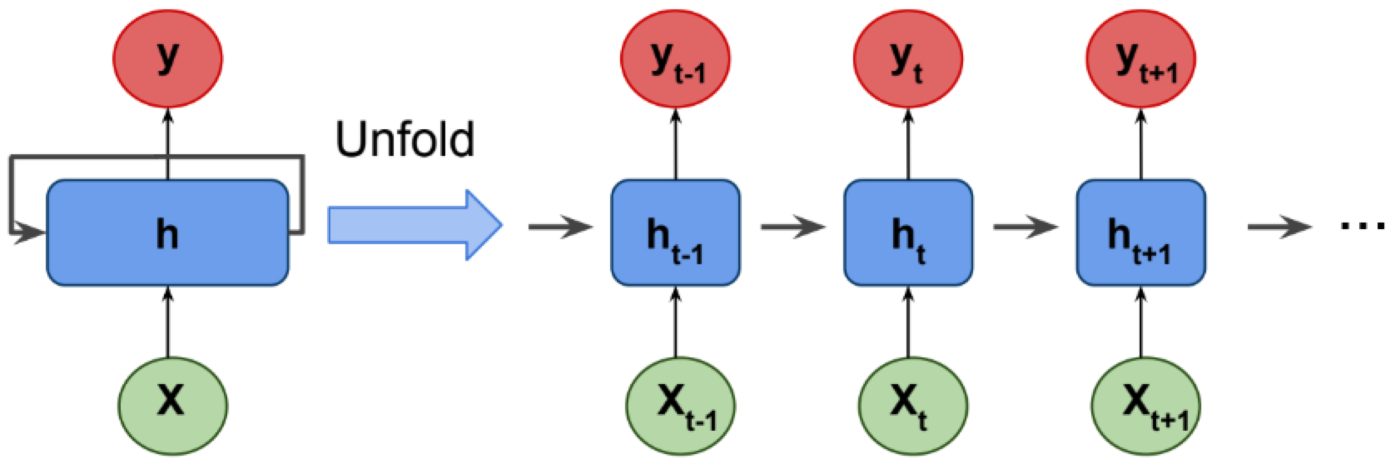
RNNs have extended their applicability based on traditional Simple Recurrent Neural Networks (SimpleRNN). Simple RNN has three layers that include input, hidden, and output layers, as shown in
Figure 1. According to the basic operating principle of Simple RNN, it connects nodes to understand current information by feeding the output of the neural network layer at time
t to an input of the same network level at time
, as shown in
Figure 1. The input data are a sequence of vectors over time
t, such as
in Input Layer. Input blocks in a fully connected Simple RNN connect to hidden blocks in a hidden layer. The hidden layer has the following hidden units
, which are connected to each other over time using periodic connections. Initializing hidden modules using small non-zero elements can improve overall network performance and stability. The concept of an unrolled structure of RNN networks has been shown as an “Unfolded” form in
Figure 1 in the case where there are multiple input time steps (X(t), X(t+1), …), multiple internal state time steps (h(t), h(t +1), …) and several output time steps (y(t), y(t+1), …).
However, these networks have their drawbacks. The first shortcoming of Simple RNN is the gradient vanishing and explosion problems. This complicates RNN learning in two ways: it cannot handle very long sequences if tanh is used as the activation function; it is very unsteady if the function ReLU is used as the activation function [
36].
Long Short-Term Memory (LSTM) is a specific architecture of the Recurrent Neural Network (RNN) that has been developed to solve the vanishing and exploding gradient problems of traditional RNNs [
12,
38]. They have shown successful results in predicting sequence problems, such as handwriting recognition, language modeling, image captioning, and acoustic signal classifications. Model training using LSTM networks is more accurate, and the training time is longer than other algorithms. In order to reduce the training time while maintaining a high level of training accuracy, Gated Recurrent Unit (GRU) networks have been developed. Furthermore, GRU networks are widely used in classification tasks [
35]. In this paper, we propose to study SimpleRNN, LSTM-based RNN units, and Gated Recurrent Unit (GRU) models in the single and stacked architectures for the UAV acoustic representations classification task since these models have been used more efficiently in the learning of sound-based recognition systems.
3.1. LSTM
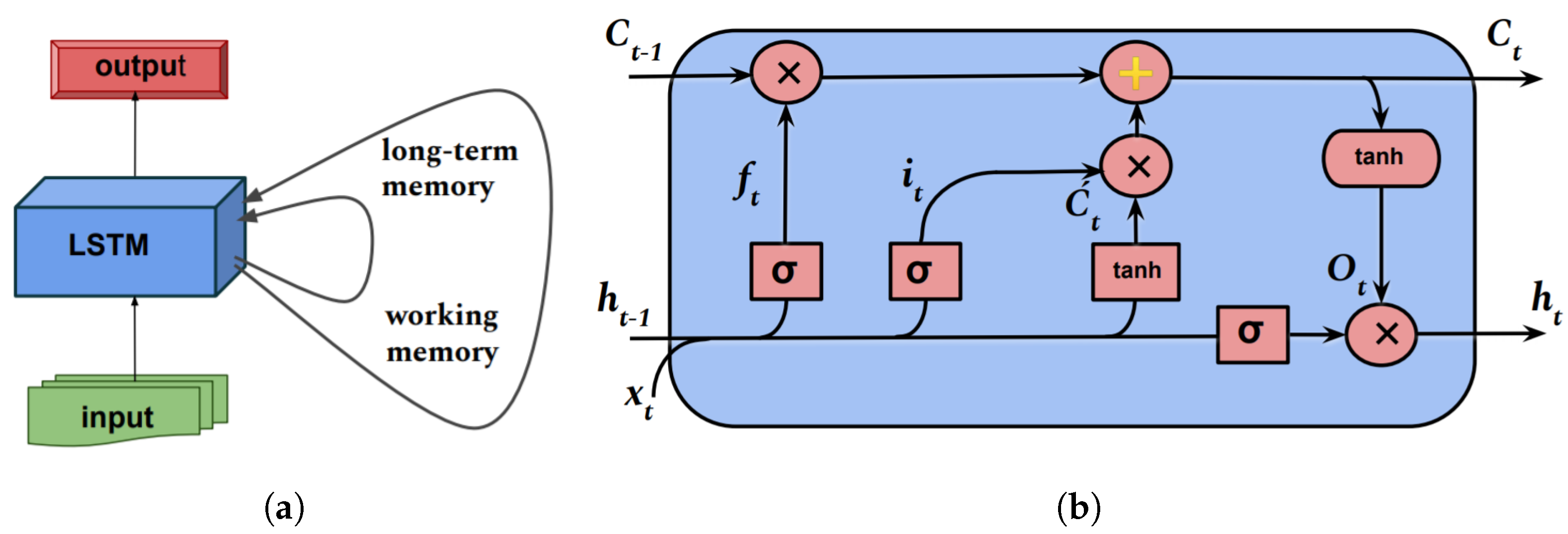
LSTM is a recurrent neural network architecture that replaces the standard layers of the neural system with long-term memory cell blocks to avoid the problem of long-term dependency; see
Figure 1 and
Figure 2. The cell blocks of common LSTMs are composed of four interacting layers: a cell state, an input gate, an output gate and a forget gate. The sequence data
of feature extraction is combined with the output data of the previous cell
. This combination of input data goes through the forget gate (1),
, and the input gate (2),
. Both gates have sigmoid activation functions to output values between 0 and 1.
Therefore, the forget gate (1) decides what information to throw out of the cell, and the input gate (2) decides which values from the input to update. Furthermore, that combination is squeezed by the tanh layer,
. Here,
,
,
are weights for the respective gate neurons; and
,
,
are biases for the respective gates. LSTM cells have an internal loop (cell state) consisting of a variable
(4) called the constant error carrousel (CEC). The old cell state
is connected to establish an effective recurrence loop with the input data. The compressed combination
is multiplied × with the input gate data
; see
Figure 2b.
However, this recurrence loop is controlled by a forget gate, which determines what data should be stored or forgotten on the network. The addition method ⊕ reduces the risk of gradient vanishing instead of multiplication. Then, the system positions the cell state via the tanh function to push the values between −1 and 1 and multiply it by the output of the sigmoid gate (5). Thus, this gate (6) determines what values should be output from the cell as the output value. On the whole, the forget gate and the input gate are used for updating the internal state (4). The main disadvantages of LSTM networks are the higher memory requirements and computational complexity than a simple RNN due to multiple memory slots. It differs from conventional RNNs in its long-term dependencies and robust advantages over gradient vanishing.
In summary, if we summarize LSTM benefits, it overcomes vanishing and exploding gradients and allows memory to overcome long-term time dependency problems with input sequences [
12,
39].
Bidirectional LSTM
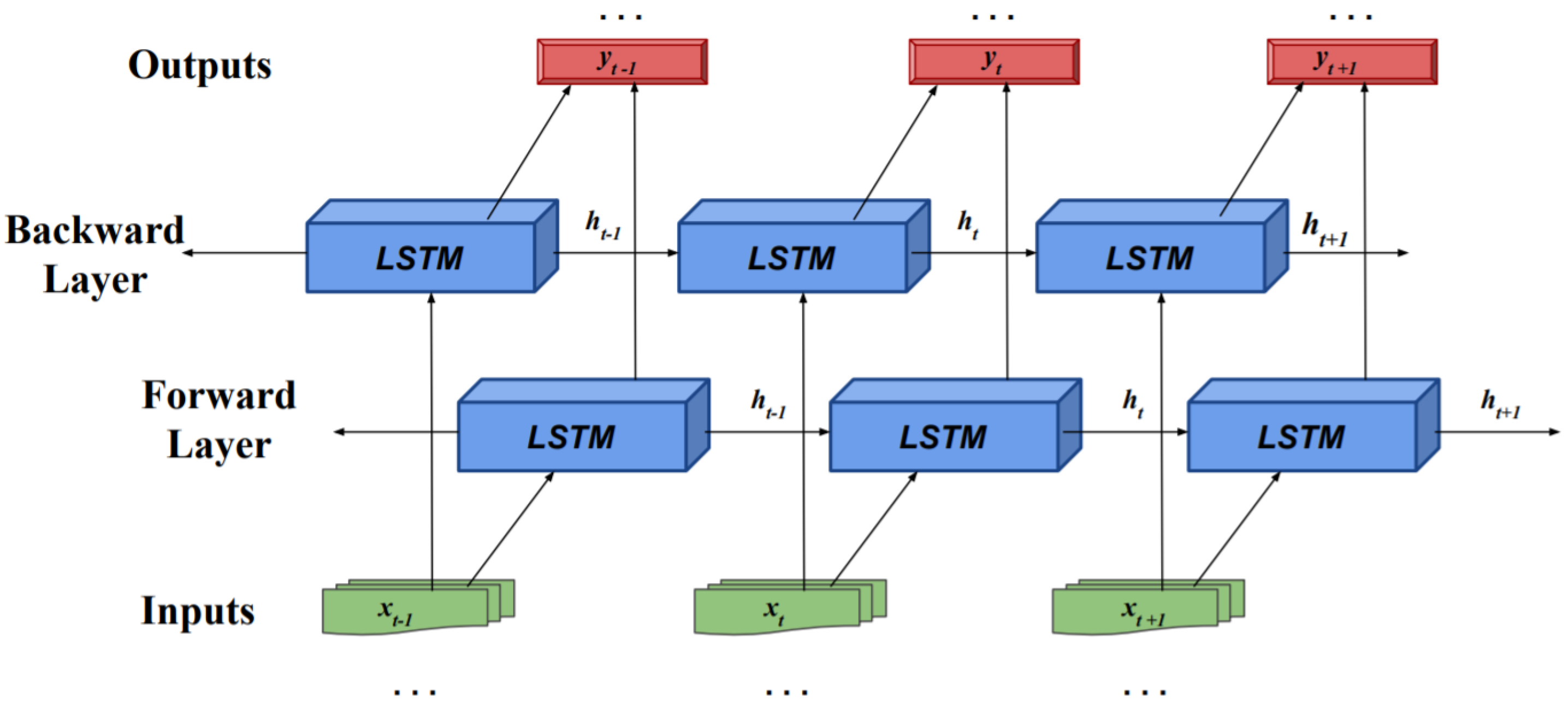
Bidirectional LSTMs are a development of typical LSTMs that can increase model performance in sequence classification tasks. With all the time steps of the input sequence, bidirectional LSTMs train two LSTMs instead of a single LSTM in the input. Bidirectional LSTMs solve the problem by outputting data from the input sequence in the forward and reverse directions over time steps.
In practice, this architecture duplicates the first recurrence level in the network by having two layers side by side, then providing the input sequence as it is at the input of the first level and providing a reverse copy of the input sequence to the second layer input. Thereby, this additional context makes the results faster [
12,
40]. Therefore, the BiLSTM network processes
sequence data in the forward and reverse directions using two separate hidden layers, and their hidden layers are connected with the same output layer; see
Figure 3. Like the LSTM level, the final output of the Bidirectional LSTM level represents the vector
, in which the last element,
, is the predicted sequence for the next time steps. BiLSTM shows its disadvantage by increasing computational complexity over LSTM due to forward and backward learning. Their main advantage is that they better reflect both future and past contexts of the input sequence than LSTM networks.
3.2. Gated Recurrent Unit (GRU) Networks
While the LSTM network has proven to be a viable option for preventing gradients from disappearing or exploding, they have higher memory requirements given the multiple memory locations in their architecture [
36]. As a solution to this problem, the GRU network was developed by the authors [
41] with less learning time due to fewer parameters than the LSTM structure while maintaining high accuracy. Unlike LSTM networks, GRU networks do not have an output gate [
35].
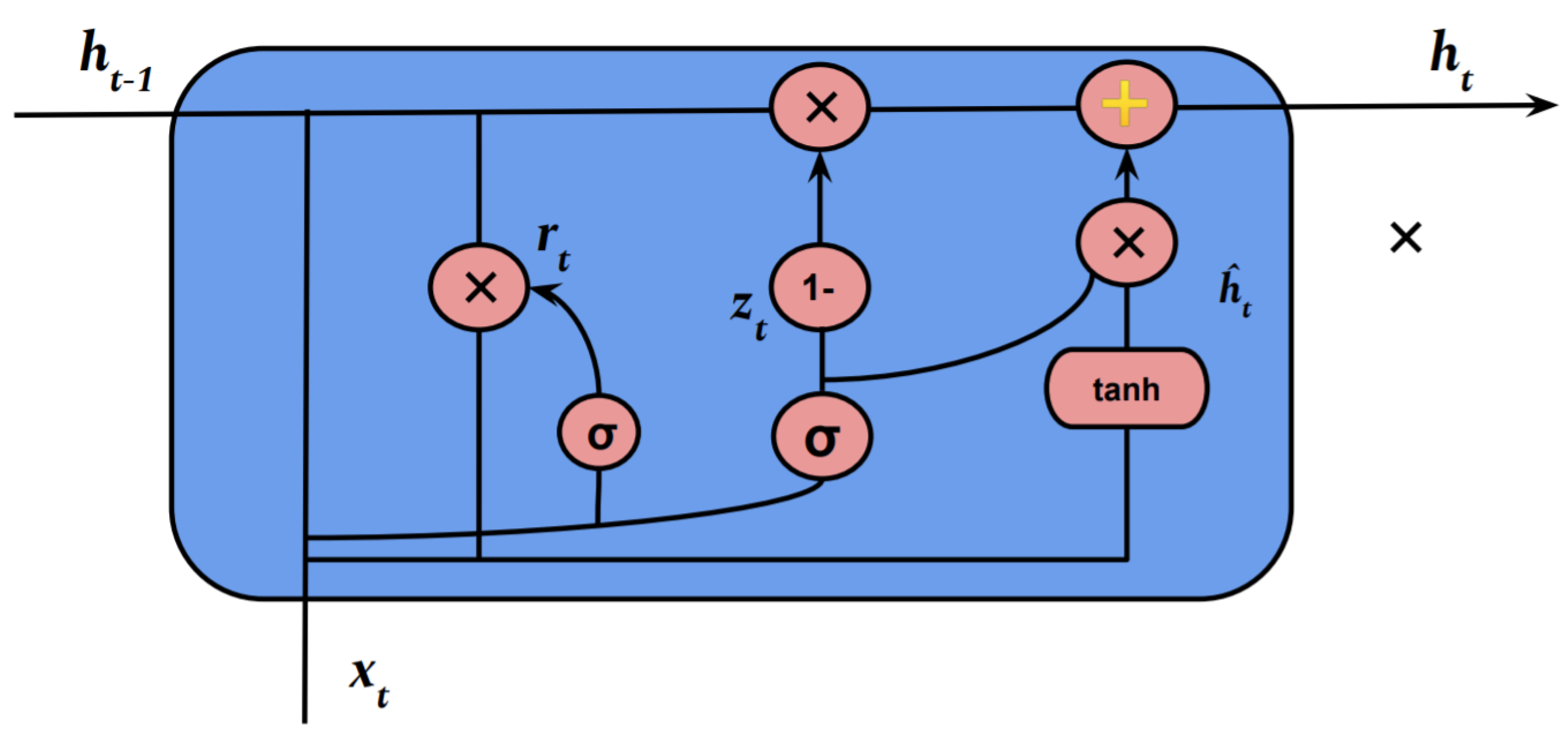
Figure 4 demonstrates the network structure of GRU. In the structure of GRU networks, at each moment of time, there are two input functions, which include the previous output vector
and the input vector
. Each gate output can be taken through a logical operation and nonlinear transformation of the input. The ratio between output and input can be characterized as follows:
where
is the update gate vector,
is the reset gate vector,
and
are weight matrices for the respective gate neurons.
is a sigmoid function and
is a hyperbolic tangent [
2,
34].
In this structure in
Figure 4, the hidden state ignores the previous hidden state when the reset gate is close to 0, and it only resets with the current input. This allows the hidden mode to remove any information that is not important in the future, thus providing a more compact view. In addition, the update gate controls how much information from the previous hidden state will be transferred over to the current hidden state. This works in the same way as LSTM memory cells and allows the RNN to store long-term information. Since each hidden module has a separate reset and update gate, each hidden module will learn to catch dependencies at different time scales. Modules that learn to capture short-term dependencies will have a reset gate that is often active, but modules that collect long-term dependencies will have an updated gate that is most active [
41].
Higher computational complexity and memory requirements than Simple RNN due to the many hidden state vectors show the disadvantage of GRU. The advantages of GRU networks, such as the ability to model long-term dependent sequences, resistance to gradient reduction, and lower memory requirements, have expanded their field of application in practice. Taking into account all the features of computing modules of RNN networks discussed above, this paper intends to carry out practical research for the UAV sound recognition task.
3.3. Single-Layer (1L) RNNs
Single-layer (1L) or Vanilla RNNs are simple configurations that consist of an input layer, a fully connected SimpleRNN/LSTM/BiLSTM or GRU hidden layer, and a fully connected output layer [
12].
Single-layer (1L) RNNs have the following properties: a sequence classification due to multiple distributed input time steps; the memory of accurate input observations for thousands of time steps; sequence prediction as a function of previous time steps; resistance to inserting random time steps into the input sequence; resistance to placing signal data on the input sequence.
3.4. Stacked RNNs
The Stacked RNN or Deep RNN network is a model that consists of multiple hidden SimpleRNN/LSTM/BiLSTM or GRU layers, where each layer contains multiple memory cells. Stacking hidden layers makes the model deeper and, more precisely, earns a description as a deep learning method. The depth of neural networks is usually explained by the success of the approach in a wide range of complex prediction problems. The depth of the network is more important than the number of memory cells in a given layer to model skill. A stacked RNN is currently a suitable method for solving sequence prediction problems [
42].
Concluding this section, our approach involves a practical consideration of the cognitive skills of RNN structures. In the course of empirical experimental work, single-layer or vanilla and stacked layers were studied to improve the accuracy of the problem. As a result, it was sufficient to use single RNN layers due to the proposed model structure. All details of the proposed model will be discussed in the next section.
4. Proposed Real-Time System
The creation of intelligent recognition systems is the main goal of the computational analysis of audio signals, which includes the study of the classification of audio events based on deep learning methods. The focus of this research work is the development of such a recognition system, namely the classification of UAV sounds for the simultaneous detection of several UAV models in the same class as unloaded UAVs when they are not loaded with payloads or their load state in the area of interest. Thus, this section aims to propose an acoustic sensor basis to create a recognition system that can detect the presence of UAVs in certain areas of interest in real-time by their sounds and recognize whether they are flying with an additional load or not. The stages of creating this system consist of the following two main parts:
The first data preparation part of the proposed work dealt with the gathering of acoustic data of unmanned aerial vehicles when they fly close and are at longer distances from microphones, as well as with and without a payload. The majority of audio data of the UAV was recorded using a professional ZaxSound SF666PRO condenser cardiomicrophone, as well as using built-in microphones from Apple products such as iPhone 11, 13, and Ipad Air (2020 release). The collected UAV sounds are grouped into three different classes. The sounds collected by a UAV flying with a special payload are called the Loaded UAV class. All the sounds of drones launched from different models were collected under the name “Unloaded UAV”, and the background noise and the sound of other objects that could be confusing were collected in the “background noise” class. The data preparation part also gathered UAV sounds from open sources. This stage was laborious due to the fact that there were not sufficient UAV sounds in known databases. This work differs from previous studies on the detection of UAV sounds in that the signal pre-processing stage, which was performed by traditional methods, is partly included in the data preparation part and inside the Recognition Framework section itself. Our approach uses the Kapre method [
8], which processes audio data on a GPU or CPU with the quick implementation of deep learning models.
The second part focused on the creation of a system itself capable of recognizing UAVs in real-time and interpreting their state during their flight. To this end, this section attempted to build a recognition system architecture using RNN neural networks, such as SimpleRNN, LSTM, BiLSTM, and GRU, by performing the task of multiple classifications of UAV acoustic data based on the concept of computer vision. Based on the ability of RNNs to successfully identify audio signals, this work was primarily intended for the practical investigation of Recurrent Neural Networks for UAV sound detection. According to previous studies on UAV sound classification and estimation in [
1,
2,
4,
42], most Drone sound recognition systems prioritize CNN networks. As can be seen from the Related Works section, reviews and full studies of all types of Recurrent Neural Networks were not investigated for UAV sounds and were not compared with CNN networks. Therefore, the main reason for the comprehensive practical study of Recurrent Neural Networks is the significant success of these networks in the study of sound (audio) signals and speech. The object of study is the processing of UAV sound data and not their images, and thus, this work considers the study of types of recurrent neural systems from a practical point of view.
Generally, previous studies of UAV sound classification [
1,
2,
4] were processed and implemented with a signal duration of different seconds on their input. This, in turn, can lead to many dangerous events over a long not-adapted duration. There was a need to develop a system capable of recognizing loaded and unloaded drones that were trained to interpret input audio signals of equal or shorter duration to represent a real-time system. Taking into account these factors, experimental work was carried out on the problem of recognizing three classes of UAV sounds with four types of computational neural cells of Recurrent Neural Networks, such as SimpleRNN, LSTM, Bidirectional LSTM, and GRU. As a result, a real-time system was developed that recognizes the sound of UAV classes trained from sound files with a duration of one second.
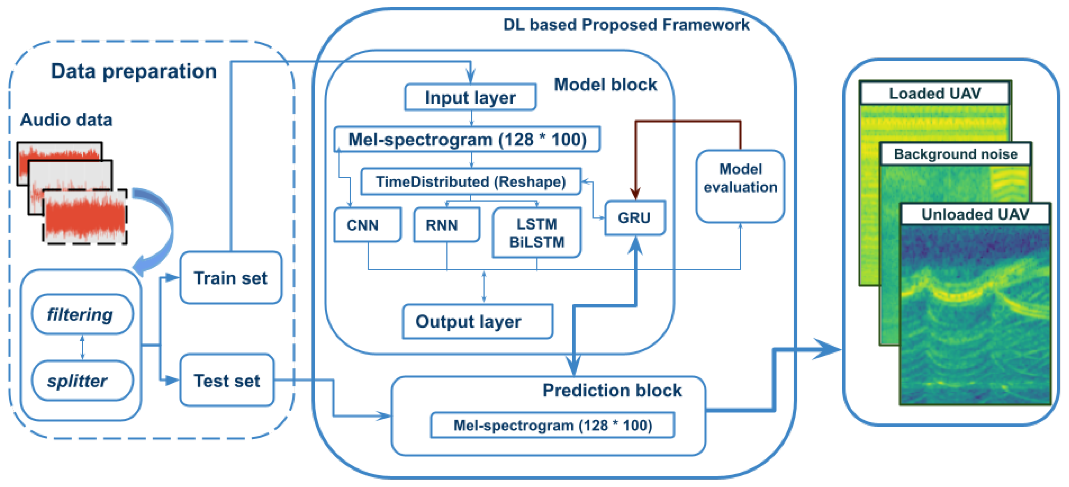
In the proposed framework, drone sounds are mainly divided into three classes and given to the input layers, as mentioned above, such as “Unloaded”, “Loaded” and “Background”. This is because, in most cases, identifying a specific type of drone does not create a meaningful need. Even though the possibility of this problem was studied in previous works [
6,
7], the problem of determining the load of the drone is a very necessary and vital system. In particular, it can be used as a solution or preventive measure for life-threatening problems, such as illegal and unauthorized transport of goods, the possibility of a load falling on people even if the load is harmless, and the transport of life-threatening goods for military purposes. Moreover, the recognition of UAV sounds can solve the problem of detecting a suspicious UAV infiltrating a strategically protected area. Determining the load of the UAV is a difficult task because it is similar to the sound of the UAV itself. The sound of flight with an additional load may differ in its matrices in the time and frequency domains and set the stage for recognition. After determining the object of study and methods, the stages of the experimental study were carried out. Accordingly, a framework for the experiment implementation was compiled, as shown in
Figure 5. Features of UAV sounds of different models and states were taken in the form of Mel-spectrograms in our work. Basically, the feature extraction step is performed by processing the signals from the time domain to the frequency domain, and these frequency data are extracted as a spectrogram, Mel-spectrogram, and MFCC [
43] coefficients. Pre-processing of raw audio data for real-time systems can be obtained using these basic time-frequency representations. In fact, most audio signals are non-periodic signals. It is necessary to take their frequency representations, i.e., the spectrum representations of these signals from the frequency domain, as they change over time. Consequently, multiple spectra are computed by performing an FFT on multiple segments of the signal window. This is called the short-time Fourier transform as in (11) [
44].
Here, K is the number of discrete Fourier transform coefficients, and g(n) is N sample long analysis window. The FFT is calculated for the overlapping signal window segments and can be obtained from the spectrogram. Typically, the signal frame duration is 20–40 ms frames. In our case, this is 25 ms. This means that the frame length for our downsampled 16 kHz signal is 0.025 ∗ 16,000 = 400 samples. The frame step or hop length is 10 ms or 160 samples, which allows for some frame overlap. The first frame of 400 samples starts at sample 0, and the next frame of 400 samples starts at sample 160 until the end of the audio signal file is reached. Periodograms are then obtained after using (12) to extract short frames from the input signals in (12):
The main reason for obtaining periodograms is to evaluate the power spectral estimate of the signal. We took the absolute value of the complex Fourier transform and performed a 512-point FFT. A unit of pitch called the Mel scale was proposed by Stevens, Volkmann, and Neumann to make equal pitch distances sound the same. In other words, the Mel scale is a pitch perception scale that is determined to be equally far from one another (after a hearing). By designating a perceptual step, the reference point between this scale and the typical frequency measurement is established. The frequencies are mathematically transformed to the Mel scale using (13).
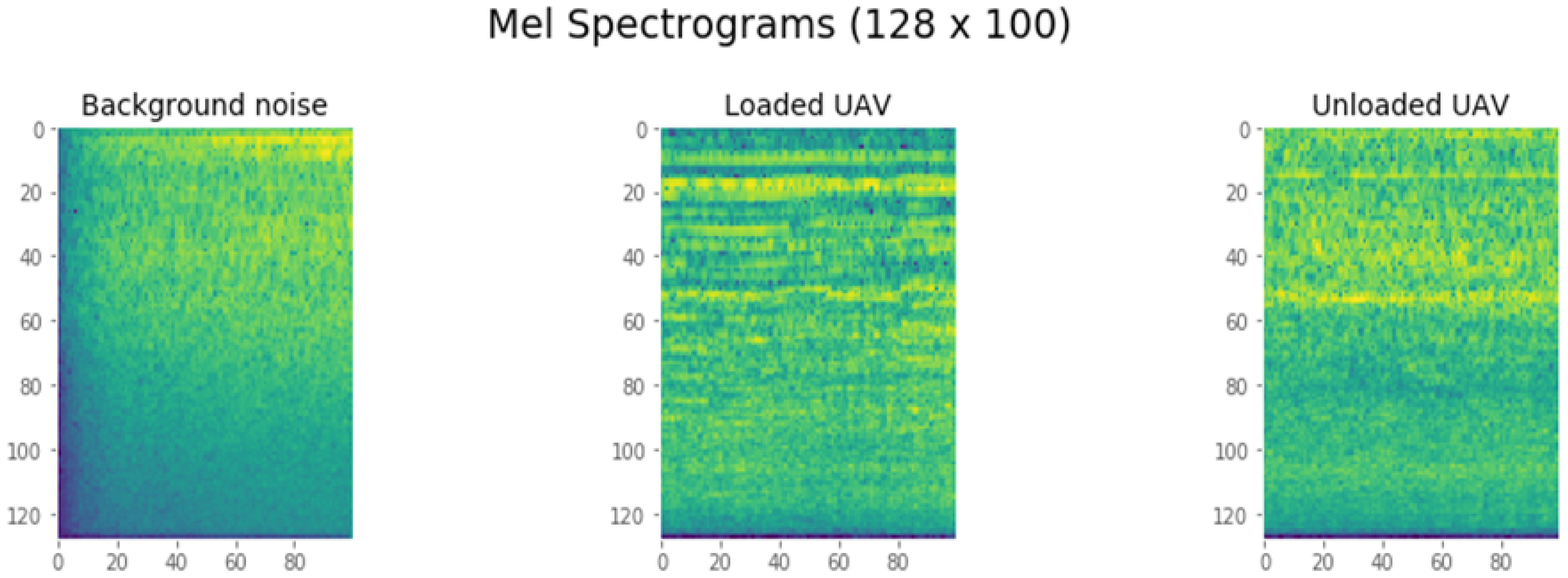
A spectrogram in which frequencies are scaled to the Mel scale is known as a Mel-spectrogram. In this work, the Mel-spectrogram was chosen as a feature extraction. It has been demonstrated through our experimental part of research that higher frequencies are shown for our UAV sounds. Accordingly, we expanded the number of filters on the Mel scale to 128. The Mel-spectrograms we chose acted as the first input layer, i.e., UAV sounds are processed as an input layer before the neural network layers, thanks to the Kapre method [
45]. Our Mel-spectrogram processed the matrices with a dimension of 128 by 100 in training time. The data of this created layer are given to the neural network, which is built further, or in each neural model, it works as an input layer that processes the input data in the network. On the other hand, it is convenient even at the training stage with the structure of RNN models for drone sounds, and also time-efficient for recognizing unseen UAV sound files for prediction. This structure can be proposed as a real-time system since the sound data can be processed and recognized using trained models from one-second duration sound data files. The proposed framework works according to the algorithm of two blocks: data preparation and training models based on the types of recurrent network cells such as single-layer SimpleRNN, LSTM, BiLSTM, and GRU,
Figure 5.
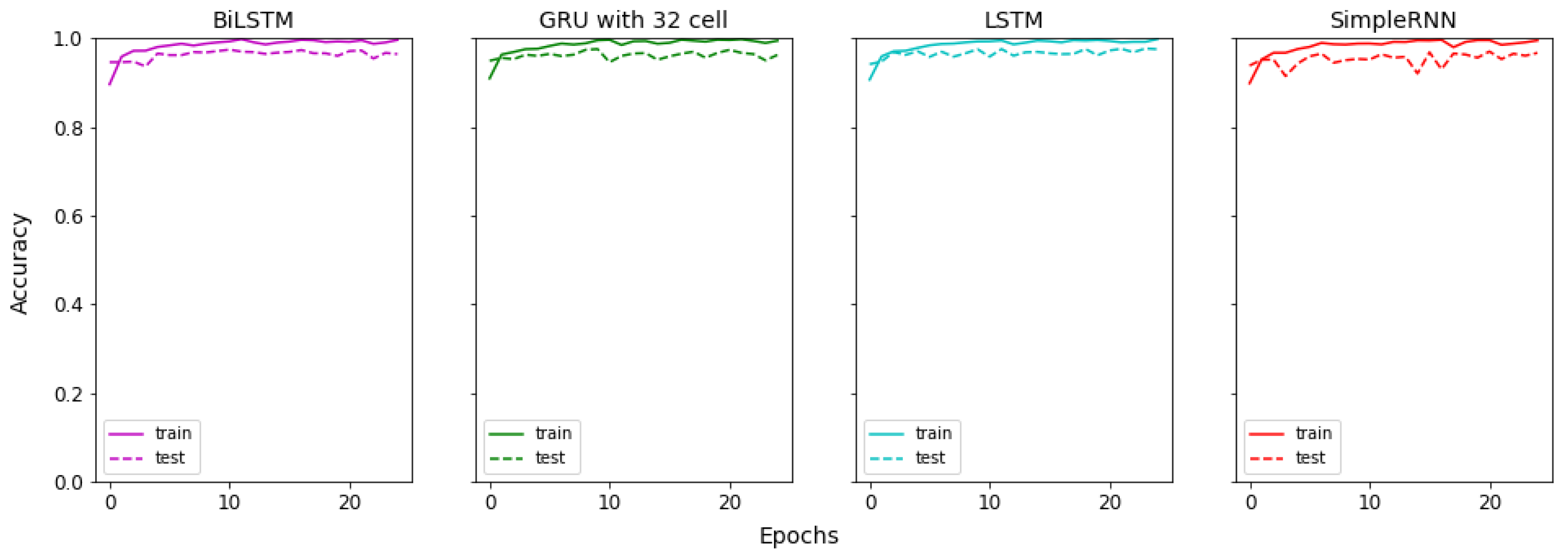
The Data Preparation section processed and split the UAV sound data for model training and predicting the models to be built. This was discussed in more detail in the Data Preparation section. Drone sounds for model training are fed as one-second audio data to Recurrent Neural Network models or CNN. Only 70% of the total volume of sound files received here is given to the training models, while the remaining 30% is stored without being shown to the models. The reason is to check the reliability of the created models. In addition to these 30 percent test files, 100 files of one-second duration for each class were saved separately, resulting in 300 files in total to test whether the models can recognize each class efficiently and reliably. As a result, the reliability of the created models for real-time systems was tested in several directions, that is, 30% of the data for the training models were comprehensively tested using model accuracy plots, and the separately stored 300 files were predicted using the confusion matrix, F1, recall, and accuracy for effective recognition of each class. The models were created on the basis of SimpleRNN, LSTM, BiLSTM, and GRU computational cells. In addition to the four models of Recurrent Neural Networks, a CNN model was created in accordance with their structure. Therefore, a total of five models were created. As mentioned above, the input layer of each model was the Mel-spectrogram layer, which performs real-time calculations. The full structural explanation and hyperparameters of the generated models are discussed in the model preparation subsection. The problem of determining the effectiveness of one of the models and the reliability of the constructed models specifically for real-time systems is discussed in the Experimental Results and Discussion section.
4.1. Data Preparation
Data preparation is an integral part of any deep-learning-based system. The Data Preparation section first started with collecting drone sounds from different scenarios, as shown in
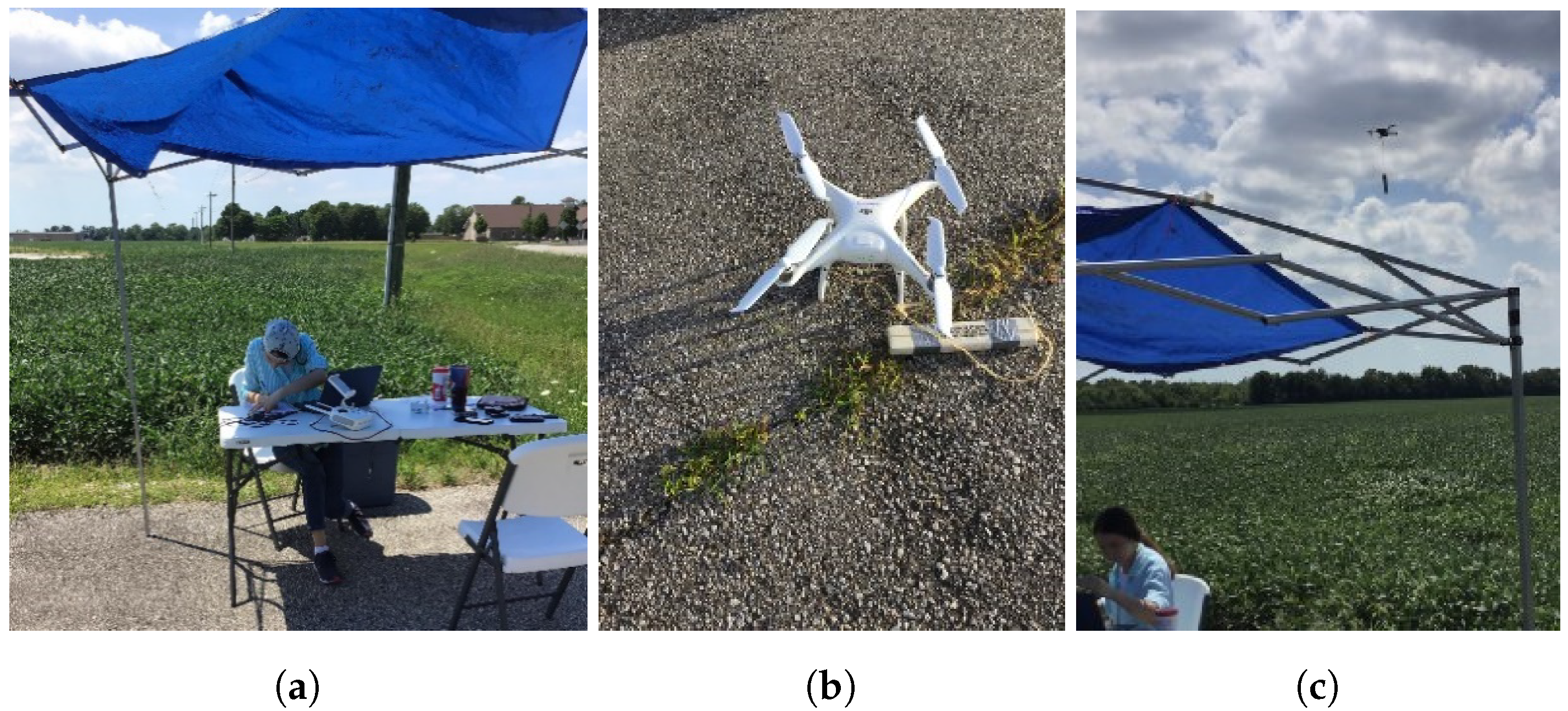
Figure 6. The main content of the database was created by testing the flights of DJI Phantom 1 and DJI Phantom 2 without and with a load at a distance of 2–100 m from the microphone. The microphone is placed on a table height of 75 cm. During the launch of the UAVs, motorcycles, gator utility vehicle riding, and a freight train were seen moving with overlapping sounds in the area. In addition, wind, canopy whispers, and other ambient sounds were heard during the test time, and their data were also collected to distinguish UAV sounds from false negatives. The loaded UAV was flown carrying a 0.5 kg payload of modeling clay at this location using the DJI Phantom 2. At the next location, the UAV Syma X20, which is widely used for recreational purposes, was flown with 0.425 kg of an iron power bank for its loaded case and also in the unloaded case. The task of load assessment of these recreational or toy drones was considered as the probability of danger with an error while controlling the drone. Other affordable UAVs, such as Syma x5c in 2–90 m and Tarantula x6 in 2–50 m distance, were tested for unloaded UAV cases. The sounds of drones DJI Phantom 4, DJI Phantom 4 Pro, Mavic Pro, and Qazdrone were also recorded. Background sounds from their launch were also collected. Not all drone models could fly with additional payload. The data of the drone that was able to fly with a load are shown in
Table 1.
All these UAVs were recorded with a 16-bit resolution of microphone depth with a frequency of 44,100 Hz, back and forth, up and down, and at different speeds by default from their technical characteristics, starting at close proximity to the microphone and the parking lot next to it. The rest of the data were obtained from open sources. Compiling audio files from open sources took much more time and additional work. This is due to the fact that the sounds of the loaded UAV were found only in amateur videos and processed using a special converter at a frequency of 44,100 Hz and a depth of 16 bits because our prediction system was based on an acoustic sensor capable of listening with a frequency of 44,100 Hz and a depth of 16 bit.
Our model was constructed to receive audio data through the wav extension and the remaining data from the open sources, which in other formats have been converted to a 44,000 Hz sampling rate with 16-bit depth resolution and “mono” mode of a microphone with the extension “.wav”. The previous studies [
1,
2] were limited by considering only a single model of UAV, which is the DJI Phantom 2. This work aimed to study the influence of various UAV models’ acoustic data on the problem of UAV load estimation. Thus, all data were collected using several types of UAV models for each of these three main classes, i.e., “Unloaded”, “Loaded” and “Background noise”. The duration of the recorded drone sounds varied from a few seconds to over 5 min. A general view of the duration of the sounds collected for each class is given in
Table 2 in seconds.
Some UAV sounds from open sources were in “stereo” mode. Some parts of the sounds of the Qazdrone, DJI Phantom 2, DJI Phantom 4, and DJI Phantom 4 Pro drones were recorded using the Apple iPad and Apple iPhone 11 and 13 built-in microphones during the experiment. All these data files were converted to 44,100 Hz and “mono” mode with a specially designed filter, run through signal envelope methods, and converted to 1-second files, which are eventually saved in special folders. As mentioned above, this work differs from previous studies on the detection of UAV sounds in that the signal pre-processing stage, which was performed by traditional methods, is partly included in the data preparation part and inside the Recognition Framework section itself. Our approach uses the Kapre method [
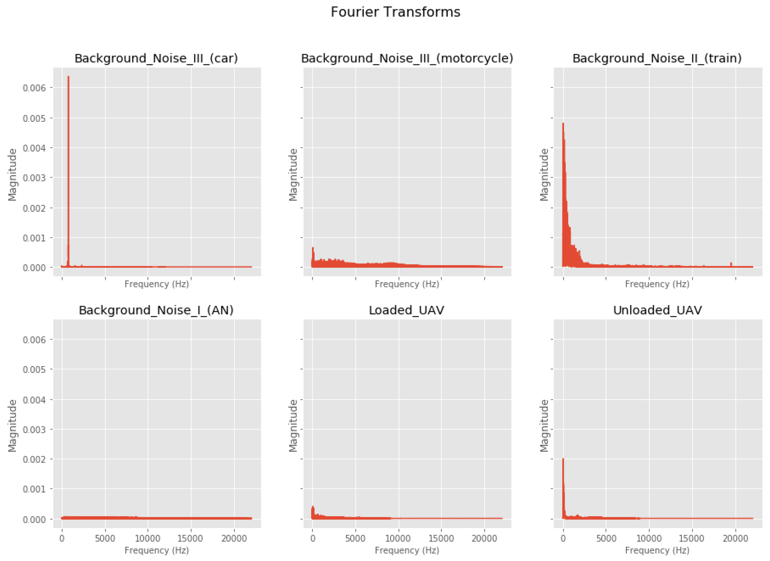
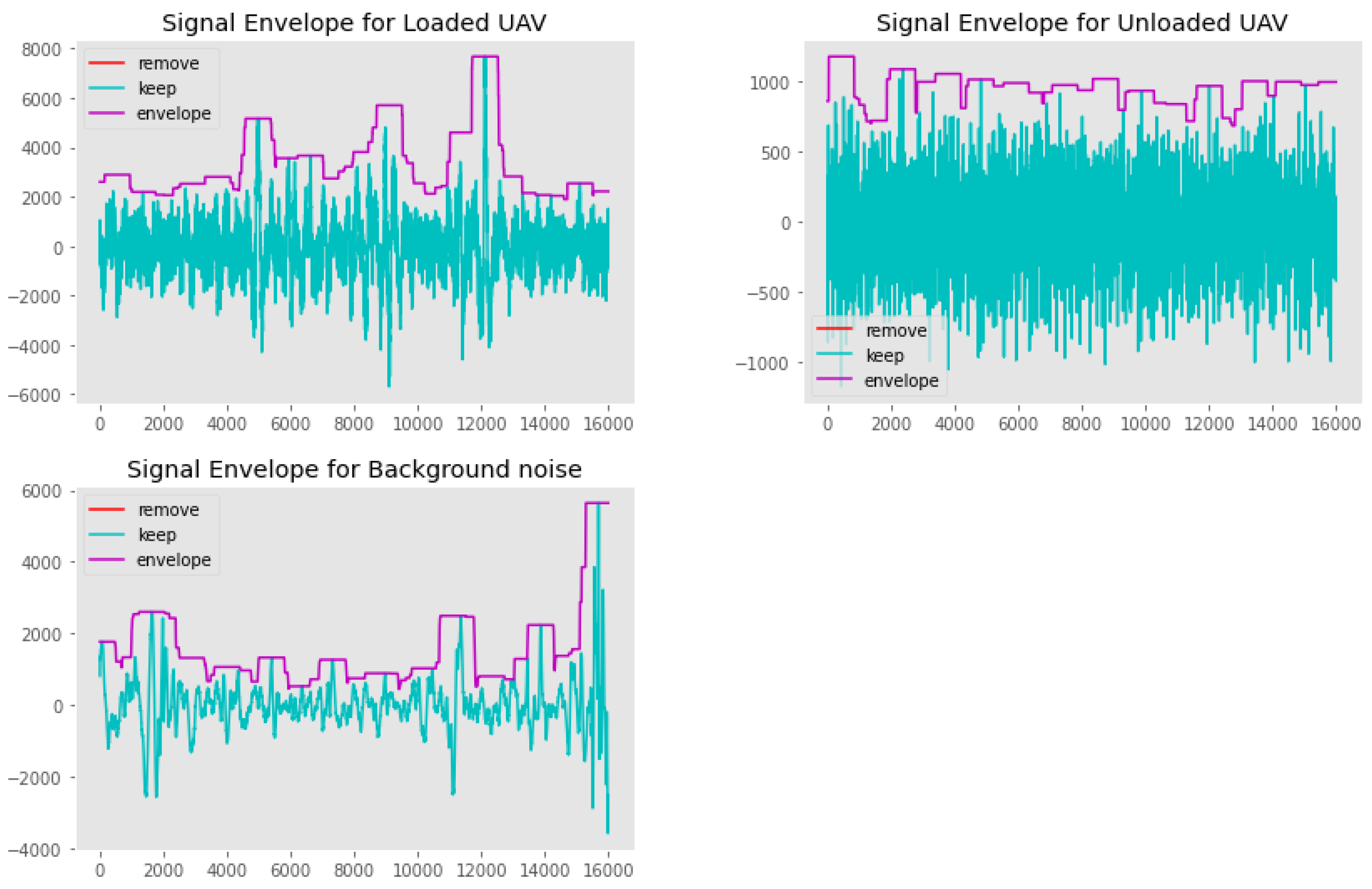
45], which processes audio data on a GPU or CPU with the quick implementation of deep learning models. Traditional methods of sound recognition systems required preliminary processing of input signals before applying them to neural networks using additional functions to obtain their time and frequency characteristics, which took some time and effort. All collected audio data were analyzed first in the time domain and then in the frequency domain. This is due to the fact that it was necessary to consider in advance the extent of all audio files, such as the sounds of UAVs and other motorized objects, which can be confused with UAVs or other background noises. So, to distinguish UAV sounds from the background noise of motorized objects such as trains, cars, and motorcycles, sound plots were plotted in the time domain (
Figure 7) and frequency domain (
Figure 8) with extended background noise classes for the investigation of information domains. The reason was the need to see and analyze the intervals of their information parts before the Framework architecture.
As can be seen in the frequency domain, the information part of the UAV sounds and the background noise we need is reflected only up to 16,000 Hz. A specially created filter program was prepared to cut off up to 16,000 Hz and, furthermore training files were planned to prepare for the model with three classes for a real-time system. The sound of some types of train signals, which were background noise, had high frequencies, but our target UAV sounds did not exceed 16,000 Hz, so only this range was captured. Objects such as motorcycles, trains, and motorized cars can potentially be confusing with the sound of UAVs. They were only analyzed separately as an additional extended background sound in the time and frequency domain during the analysis step temporarily as mentioned before. In the case of the task of recognizing train sounds, it is possible to increase the frequency range. As a guideline when examining other motorized objects, we have tried to show the extended classes of background noise objects. However, according to our task, it was adapted to the sounds of the UAV.
After selecting the required frequency range at the analysis step, the sound base was again combined into three classes using a special filter that cuts off all signals below 16,000 Hz. And the features of the Mel scale were obtained in the proposed structure itself using a range of time and frequency hyperparameters from the analysis part. Temporal and frequency characteristics based on traditional methods conducted in Python are mainly implemented using libraries Librosa and Essentia [
45] in many studies. Our work involves the use of the Kapre method, which is developed as Keras layers. The research work was carried out using the python program using the layers and libraries of Keras, including KAPRE. The main advantage of the Kapre method is the optimization of audio signal processing parameters. In addition, the time and frequency representations, their normalization, and data augmentation are performed in real-time on GPU or CPU. However, it is necessary to analyze the sounds of various objects in the frequency domain in order to pre-determine the parameters of the filters up to the Kapre layers due to the characteristics of their natural appearance. In order to perform this preliminary analysis task, we obtained spectra performed individually for each class in the frequency range using Fast Fourier Transform (FFT) for our time domain signals above. Most of the changes in the audio signals are observed at low frequencies, and the downsampling step is performed at a frequency of 16,000 Hz, preserving some informative areas of signals for objects of all classes. Thus, in the next step, we divided all signals into one-second chunks from the entire duration of all audio recordings, as we are trying to build a real-time system. Therefore, our audio files need to be trained using 1-second audio files. In addition, a signal envelope method was performed to eliminate dead zones in sections of one-second duration, i.e. lower values with zero thresholds were cleaned up by creating our special filter in
Figure 9.
This work is approached based on the image classification method, while its neural networks have the ability to differentiate objects based on feature vectors of all classes, especially by allowing background noise to be recognized as false negatives. The spectra of the signals that have passed the above-mentioned cleaning function are shown in
Figure 9. Through empirical research, the Mel-spectrogram was chosen as an effective frequency representation for a real-time recognition system. The Mel-spectrogram parameters are shown in
Table 3 in the Model Preparation section.
In conclusion, this subsection collected UAV audio and background noise data and only analyzes the signals in the time and frequency domains to find the interval of the information domains. As a result, a filter was created that collects 1-second audio signals below 16000 Hz into three classes. And the frequency characteristics of the Mel scale used for the system have not been obtained in this subsection. This is because it will be taken immediately as the first layer of the proposed structure in the next subsection.
4.2. Model Preparation
This subsection attempts to build recognition models using RNN neural networks, such as SimpleRNN, LSTM, BiLSTM, and GRU. The task is performed on the basis of multiple classifications of UAV acoustic data based on the concept of computer vision. This is because the UAV audio data are entered as one-second audio data in the input and form the Mel-spectrogram layer using the Kapre method [
45]. The output launches a stream of images created from frequency representations, called a Mel-spectrogram, to the next level, as shown in
Table 3.
The Mel-spectrogram is a layer of Kapre that is expanded on a spectrogram by multiplying the conversion matrix of the Mel scale from linear frequencies [
45],
Figure 10. Our approach has studied a large range for the Mel-spectrogram layer, as shown in
Table 3. As a result of the experimental attempts, 100-time vectors and 128-frequency features were obtained. These selected layers in the proposed structure were chosen for their following features, and the hyperparameters were chosen through a series of experiments: the normalization layer is implemented in these Mel-spectrograms as the second layer of the model as it normalizes two-dimensional input data per frequency, time, batch, and channel. When the input vectors have already been selected, the TimeDistributed(Reshape) layer is used to ensure that the size of the matrix provides data to the layers of the RNN. A neural dense layer with the tanh function was added to approximate the size of the matrix to the size of the RNN cells. As the fifth layer of the model structure, computational units such as SimpleRNN, LSTM (Long-Short Term Memory), BiLSTM (Bidirectional LSTM), and GRU (Gated Recurrent Networks) networks were connected with 32 cells. A concatenation layer was added after the RNN cells, and then the dense layers were connected based on the hyperparameters in
Table 3. The MaxPooling1D layer was placed after the RNN layer to make the architecture easier to learn. Then, a 32-cell dense layer with a ReLU function was created. In addition, a Flatten layer was used to make the multidimensional output linear and transfer it to a dense layer. The output of the Flatten layer is carried over to the next layers for the classification task. A Dropout layer is added to the next row so that the model does not overfit and showed a good fit when evaluating the model with a coefficient of 0.2 for a 32-cell RNN. A dense layer of 32 cells with an activity regularizer and ReLU function was added before the final dense layer. It should be noted that the activity regularizer function had a great impact on the representativeness of the accuracy graphs in model training for the given UAV sounds. Therefore, this function was considered within 0.01–0.00001. The number of dropout layers was changed according to the number of RNN cells. In the case of GRU, with an increase in the number of cells to 64, a change in the dropout coefficient from 0.25 to 0.3 was considered since the model could be retrained. In the realization of the models, the “categorical cross-entropy” loss function is optimized for the multiple classification task.
The “Adam” implementation of gradient descent is used to optimize the weights, and the classification “accuracy” is calculated during the model training, validation, and testing to evaluate learning-skill and generalizing-skill, of models in comparison to all architectures. The results of these investigations are given in the Training and Evaluation Metrics subsections.
To summarize this section, the design of the proposed structure has been adapted for training with RNN training cells and additional layers by obtaining spectrograms based on the Mel scale and other hyperparameters using
Table 3.
6. Conclusions
In this study, we investigated architectures such as SimpleRNN, LSTM, bidirectional LSTM, and GRU based on a practical application for a real-time UAV sound recognition system. We paid special attention to determine whether the UAVs were loaded or unloaded. In general, UAV sounds were collected into three main classes: loaded UAVs unloaded UAVs, and background noises, including the sound of other engine-based objects from the scene. In the next stage, we tried to assess the level of accuracy of the UAV recognition system using all the metrics of multiple class classification tasks. As a result, the GRU architecture (64) was found to be an efficient model with a high degree of predictability. According to our goal, this model can recognize loaded UAVs and unloaded UAVs with 98% accuracy and background noise with 99% accuracy. This evaluation ensures the ability of the UAV sound recognition system at a reliable level, suggesting the creation of an array of acoustic sensors using the proposed GRU model (64). Other RNN network architectures are robust for binary classification problems. Thus, based on the predictions, SimpleRNN, LSTM, BiLSTM, and GRU architectures can be used in the UAV load detection task due to their better content-based recognition ability than CNN models. The CNN model could only detect cases of binary object classification and was slightly smaller than RNN networks. Within this study, our work contributed to the following solutions:
(1) The hyperparameter size of the “good fit” Mel-spectrogram for UAV sounds was developed during an empirical experimental study.
(2) The structure of RNN networks based on the “best fit” hyperparameters and fewer layer-based structures has been developed for real-time systems.
(3) A real-time recognition system was adapted for UAV states when they have different masses of weights.
(4) For the first time, all RNN cell types were examined in one study to provide guidance on the choice of these cell types for other types of sounds.
This work was limited by the low amount of acoustic data of the loaded UAVs. However, this work has shown that UAV loads can be determined and estimated in real-time. The future work of our study could focus on two areas: first, increasing the loaded UAV’s audio dataset and exploring in detail the distance-based detection problem.
