Article

Stability Derivatives of Various Lighter-than-Air Vehicles: A CFD-Based Comparative Study

by
Anoop Sasidharan
1,
Ratna Kishore Velamati
2,*,
Sheeja Janardhanan
3,
Venkata Ramana Murthy Oruganti
1 and
Akram Mohammad
4
1
Department of Electrical and Electronics Engineering, Amrita School of Engineering, Amrita Vishwa Vidyapeetham, Coimbatore 641112, India
2
Department of Mechanical Engineering, Amrita School of Engineering, Amrita Vishwa Vidyapeetham, Coimbatore 641112, India
3
School of Naval Architecture and Ocean Engineering, Indian Maritime University, Visakhapatnam 531035, India
4
Department of Aerospace Engineering, King Abdulaziz University, Jeddah 21589, Saudi Arabia
*
Author to whom correspondence should be addressed.
Drones 2022, 6(7), 168; https://doi.org/10.3390/drones6070168
Submission received: 15 June 2022 / Revised: 5 July 2022 / Accepted: 6 July 2022 / Published: 7 July 2022
(This article belongs to the Special Issue Honorary Special Issue for Prof. Max F. Platzer)

Abstract

:
An aerostat with a single tether is proposed for the application of wind measurements at low altitudes. In the current study, the aerodynamic model parameters (stability derivatives) of the aerostat are investigated based on a CFD-based approach. The static, as well as the dynamic stability derivatives of the aerostats are presented. The calculation of the dynamic stability derivatives involves the simulation of the oscillations of the aerostats in their axial direction (surge), the vertical direction (heave) and angular motions with respect to the lateral direction (pitch). A forced sinusoidal oscillation is used for the simulation of the aerostat, and one stable period of oscillation is taken for the derivatives’ extraction. Four different aerostats are considered for the current study with four different angles of attack. The Zhiyuan aerostat, HAA aerostat, NPL aerostat and GNVR aerostat are the aerostats considered for this study. The stability derivative results obtained for the four aerostats are analyzed and compared with respect to their geometrical features. From the static aerodynamic characteristics, the Zhiyuan aerostat shows better performance than the other aerostats in terms of the lift–drag ratio. The dynamic stability derivatives of the Zhiyuan aerostat suggest its application as the proposed low-altitude wind measurement system.

1. Introduction

Being a fast-growing nation, India plans to make the share of renewable energy in the power system around 40% by 2030. Developments in wind-energy-harvesting methods aid this vision along with other renewable resources such as solar, tidal and geothermal energy. Wind energy is one of the essential renewable energy sources in the Indian power system. The National Institute of Wind Energy (NIWE) estimated the wind power potential of India at 100 m above ground level as 302 GW. This is a sign that wind energy will play a significant role in India’s energy sector in the coming years. The site selection, turbine altitude selection, tower structure design, alignment of wind turbines in the farm, estimation of the expected power output and the extension of existing wind farms are highly dependent on the wind data of the intended site. Even after the installation of the wind farm, hourly, daily and long-term wind data are required for the dispatching of load, forecasting the demand for load, forecasting/planning of the generation and design of the supporting fixtures.
The traditional method of wind data collection in wind-energy-harvesting sites is based on pole-based methods. This method has a few drawbacks, such as the need for a permanent structural setup, which may cause environmental and aesthetic impacts on the site, the inability to vary the altitude of the structure and a long gestation period, and it cannot be relocated or reused easily [1]. There are other methods that are not so popular such as the satellite-based methods [2], LiDARs [3] and measurements using flying vehicles [4].
The current research proposes an alternate method for the low-altitude wind measurement using a tethered aerostat. A ground station for the tether control, powering and data transfer, a tether for keeping the aerostat connected to the ground station, the payload for the wind measurement and the aerostat are the significant components of the proposed system [5]. Compared to the conventional method, the proposed method has the following advantages: it gives freedom to vary the altitude of operation; it does not require any permanent structure for the deployment; it takes less time for deploying at a site and can be relocated easily to different locations and reused.
As the wind farm sites are highly prone to disturbances such as wind gusts, it will be challenging to keep the wind measurement free of errors [6,7]. Such unsteady conditions will result in oscillations or vibrations in the respective axis [8]. The previous study performed by the authors was to analyze the aerodynamic performance of the aerostat undergoing various unsteady wind conditions, as presented in [9]. The current study is part of an investigation to develop a control system for the single tethered aerostat and payload assembly. A mathematical model is necessary to analyze system stability and develop the appropriate control algorithm for the proposed tethered aerostat-based wind measurement system. This paper presents the investigation of the mathematical model parameters required for the aerostat.
Mathematical modeling of complex systems such as aerial vehicles plays a vital role in understanding and predicting the unsteady aerodynamic behavior of that system. An accurate aerodynamic model of the vehicle can improve the design and analysis of the control system required for the operation. There is some literature that presents the analytical modeling of the aerodynamics of airships or aerostats [10,11,12,13,14,15]. The model is highly dependent on the experimental data and is not generalizable for a class of vehicles. Non-linear methods estimate the wind-induced aerodynamic parameters, which are numerically complex for an aerostat [16]. Since the functional form of aerodynamic effects in the form of forces and moments on the aerial vehicle are not readily available for direct measurement, mathematical derivatives are needed to model these forces and moments [17,18]. Derivatives represent a measure of the variation of a parameter or a function with respect to the input or another function or parameter. In the field of dynamics, those derivatives that can represent the model’s sensitivity to some motion variables are termed stability derivatives because these derivatives help simplify the model so that the stability analysis and control of the model becomes easy. Aerodynamic models using stability derivatives are considered an accurate approach to the mathematical modeling of aerial vehicles. Since Bryan’s introduction in 1911, the stability derivatives have been considered the basis for modeling the aerodynamic loads in the equations of motion of aerodynamic systems [19]. Different applications of stability derivatives include linearization of the model for a steady (otherwise with small perturbations) flight to describe the vehicle’s dynamic stability, control system design, trajectory design, aerodynamic shape optimization and design and the development of flight simulators [20].
Stability derivatives can be classified as velocity derivatives and acceleration derivatives (added mass terms). The derivatives due to acceleration are usually neglected for the dynamics of the heavier-than-air vehicles because of their significantly small values. The importance of the added mass terms in a dynamic model is based on the relative densities of the body and the fluid [21]. For underwater vehicles and Lighter-Than-Air (LTA) systems (such as aerostats, airships and hot air balloons), where the added mass effect cannot be neglected, derivatives due to acceleration terms will be included as the added mass and added inertia terms [22]. Added mass, apparent mass, and virtual mass are the terms contained in the dynamic model of aerodynamic geometries moving through fluids to represent the forces and torques due to the inertia of the geometry. The second class, the stability derivatives due to the velocity of the motion variables, is usually considered along with the aerodynamic force terms in the dynamic model [23]. These terms are generally called stability derivatives, and those due to the acceleration terms are called the added mass terms.
The estimation or extraction of the stability derivatives was reported mainly using real flights, wind-tunnel testings and computational/numerical methods. Some of the essential works reported in these classes are presented here. The estimation of the aerodynamic derivatives for the LTA vehicles using a semi-empirical procedure was reported in [11]. They considered the hull–fin interference using an analytical model and the static wind tunnel data by which the dynamic motion of the vehicle can be represented well. As an extension, they investigated the longitudinal and lateral stability derivatives for the TCOM 71M aerostat [24]. The model also verified the static and dynamic stability of the aerostat obtained using the stability derivatives. A neural-network-based prediction of the dynamic derivatives of an aircraft at high angles of attack was presented by [25]. They provided decent results for pitching moment derivatives compared to the wind tunnel experimental data. A wind-tunnel-based stability derivative estimation for a hybrid buoyant aerial vehicle is presented by [26]. They compared the stability of the vehicle with wings and without wings. Even though the physical realism of the experimental methods such as flight tests and wind tunnel tests is highly appreciable, there are some limitations such as scaling errors, blocking effects and high cost. A system identification approach for obtaining the stability derivatives of an LTA vehicle undergoing swing oscillation was presented in [27]. Computational methods were also reported to estimate the stability derivatives of LTA vehicles [28].
Considering the fact that the Computational Fluid Dynamics (CFD) solvers are now capable of handling high-performance tasks due to the developments in digital computing, their application in the extraction of stability derivatives is being largely explored by the research community. Most of the limitations of the experimental method, such as the wind tunnel tests, can be overcome by the CFD-based methods [29]. A forced oscillation of the body was used for extracting the stability derivatives. The motion variables other than the oscillating parameter are considered zero as per the linear theory. A forced periodic oscillation is imposed on the respective degree of freedom of the model to calculate the respective dynamic derivative. For example, the moment stability derivative due to the pitch rate can be extracted by imposing a periodic angular oscillation about the lateral axis and center of the moment [18]. The measured moment response will be used to extract the derivative based on the Fourier series approximation. Such a methodology for estimating stability derivatives using CFD for the Zhiyuan airship is presented in [30]. Stability derivatives involved in the pitch and heave motions of the airship were investigated using forced sinusoidal oscillations. They presented the effect of the tail fins on stability as well. Stability derivatives’ prediction for a full aircraft configuration was investigated to represent the unsteady aerodynamic load on the flight dynamics for transonic speeds and larger angles of attack, as in [31,32]. An investigation of the stability of hybrid airships using the analysis of the stability derivatives was presented by [33]. The added mass and inertia terms’ extraction for an underwater vehicle was reported in [34]. They compared their results with the results from an experimental procedure and theoretical results. Using stability derivatives addressed by [35], the aerodynamic shape optimization considered the derivatives as constraints in the optimization problem.
The forced sinusoidal-oscillation-based stability derivative extraction is the most popular method due to the well-developed Fourier theory and the easy practical realization [5,23,36]. There are also works reported with different methodologies, such as the work reported in [37]. The history effect and the actuation of the body using piece-wise velocity functions were the basis for their methodology. Even though the rotational dynamics were not able to be captured, the methodology was validated with existing data. A detailed literature review of the existing methodologies for stability derivative extraction using CFD can be found in [38].
In this paper, the authors present the aerodynamic model parameter estimation of an aerostat using a CFD-based methodology. As the lateral dynamics of the aerostat are considered to be compensated by the aerostat control surfaces, the longitudinal dynamic model of the aerostat is considered in this study. Stability derivatives that are necessary for a longitudinal dynamic model of the considered aerostat were extracted by applying a translational forced sinusoidal oscillation in the vertical and axial directions and angular oscillations with respect to the lateral axis. In a previous study, the authors investigated the effect of the unsteady motion of the aerostat on the stability derivatives [9]. The current paper considers a steady wind formulation for the analysis. As the geometry of the aerostat affects its aerodynamic stability greatly, the effect of the aerostat envelope shapes in the context of stability derivatives is investigated as well. This will also help to understand the methodology’s efficacy and generalization thoroughly. There are many aerostat/airship geometries available in the open literature. The NPL shape has been designed and developed by the National Physical Laboratory to reduce the chances of flow separation [39]. This was achieved by providing a continuous variation in the radius of curvature of the profile. The GNVR shape has been reported to be a low drag profile [39]. Both of these shapes represent a combination of different simple geometries, such as ellipses and parabolas. This made geometry optimization feasible for them. A high-altitude application was reported, which was claimed to have a minimum weight to increase the payload and stability (HAA shape) [40]. All the above-mentioned shapes were proposed for stratospheric operation. A bionic design for the airship has been reported to minimize drag (bionic shape) [41]. This was achieved by imitating the morphological features of an aquatic animal (Physalia physalis). Other low-drag profiles were also reported for specific applications, such as the Zhiyuan shape [30] and Wang shape [42].
The contents of this paper can be listed as follows: The motivation and the relevant literature for the current study are presented in Section 1. The extraction of the stability derivatives involved in the mathematical model is a significant contribution of this paper. The stability derivative estimation methodology for the surge (axial), heave (vertical) and pitching oscillatory motions are presented in Section 2. There is no work reported so far in the open literature on analyzing the effect of the shape of the model on the stability derivatives. This paper contributes to such a study by considering four different aerostat shapes for the calculation of the stability derivatives. The four aerostat shapes used for the analysis are presented in Section 3. Section 4 includes the numerical simulation methodology and the simulation setup. The computational grid and the domain used for the simulation are also presented. The simulation results and discussion on the results are presented in Section 5, and the significant findings of the current study are presented in Section 6.

2. Stability Derivatives’ Extraction Methodology

A stability derivative extraction methodology based on CFD analysis was presented by the authors in [5]. The analysis was conducted for unsteady wind and unsteady aerostat motion. The current paper deals with the steady analysis of the aerostat stability derivatives and the effect of the shape of the aerostat on the stability derivatives.
In this work, the longitudinal motion of the aerostat is considered. The lateral motion of the aerostat is considered to be compensated by the control surfaces. The motion variables involved in the decoupled linear longitudinal dynamic model are u, w and q. The longitudinal model of the aerostat can be expressed as [21]
m x u ˙ + ( m a z D ˙ q ˙ ) q ˙ = D a + D T + D g m z w ˙ ( m a x + L ˙ q ˙ ) q ˙ = L a + L T + L g J y q ˙ + ( m a z M ˙ u ˙ ) u ˙ ( m a x + M ˙ w ˙ ) w ˙ = M a + M T + M g
where D a , L a and M a are the aerodynamic forces and moment, D T , L T and M T are the forces and moment due to the tethers and D g , L g and M g are the forces and moment due to buoyancy and gravity.
In the current study, the tether dynamics and the forces due to gravity are not included, and for simplicity, they are named as external forces ( F e x t ) in the rest of the paper. The aerodynamic part of the longitudinal dynamic model of the aerostat can be represented as follows:
D a = D e + D ˙ u u + D ˙ w w + ( D ˙ q m z W e ) q L a = L e + L ˙ u u + L ˙ w w + ( L ˙ q + m x U e ) q M a = M e + M ˙ u u + M ˙ w w + ( M ˙ q m a x U e m a z W e ) q
where W e and U e are the component of steady velocity along the vertical and axial direction, M e , L e and D e are the static moment, lift and drag derivatives, M ˙ u , L ˙ u and D ˙ u are the moment, lift and drag derivatives due to surge velocity, M ˙ w , L ˙ w and D ˙ w are the moment, lift and drag derivatives because of vertical velocity and M ˙ q , L ˙ q and D ˙ q are the moment, lift and drag derivatives due to pitch.
Thus, Equation (1) can be expressed in matrix form as given in Equation (3). The terms with dots are the stability derivatives involved in the aerostat’s longitudinal dynamic model.
m D ˙ u ˙ 0 m a z D ˙ q ˙ 0 m L ˙ w ˙ m a x + L ˙ q ˙ m a z M ˙ u ˙ m a x + M ˙ w ˙ I y M ˙ q ˙ u ˙ w ˙ q ˙ = D e L e M e + D ˙ u D ˙ w D ˙ q m z W e L ˙ u L ˙ w L ˙ q + m x U e M ˙ u M ˙ w M ˙ q m a x U e m a z W e u w q + F e x t
The model variables included in the longitudinal model of the aerostat are u, w, q, D, L and M. These longitudinal dynamic variables are predominant in the heave, surge and pitch motions of the aerostat.
The methodology used for the calculation of the stability derivatives includes the simulation of the model for steady-state and then transient and, finally, the oscillations in the respective directions. The forces and moment (D, L and M) are measured for the oscillated motions. A stable cycle of data is used from these measured responses to extract the stability derivatives using the Fourier-series-based method discussed in the following sections.

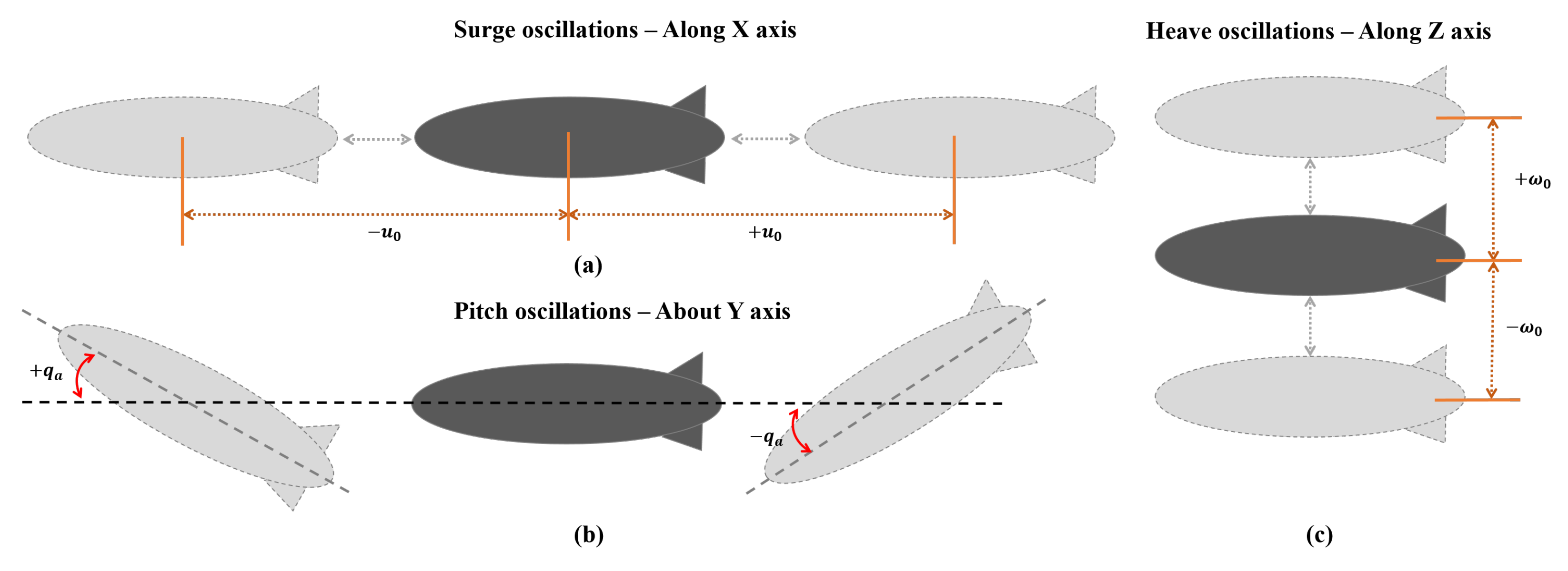
2.1. Pure Surge Oscillations

The stability derivatives associated with the translational forward motion (along the X-axis) can be expressed as the linear decomposed forces and moment as follows:
D a s = D e + D ˙ u u + D ˙ u ˙ u ˙ L a s = L e + L ˙ u u + L ˙ u ˙ u ˙ M a s = M e + M ˙ u u + M ˙ u ˙ u ˙
A forced sinusoidal oscillatory motion will be induced in the aerostat axial direction, as shown in Figure 1a. The motion is described using the displacement as x a = u a sin ω s t , velocity as u = ω s u a cos ω s t and acceleration as u ˙ = ω s 2 u a sin ω s t . Putting the variables u and u ˙ in Equation (4) will result in
D a s = D e + D ˙ u ω s u a cos ω s t D ˙ u ˙ ω s 2 u a sin ω s t L a s = L e + L ˙ u ω s u a cos ω s t L ˙ u ˙ ω s 2 u a sin ω s t M a s = M e + M ˙ u ω s u a cos ω s t M ˙ u ˙ ω s 2 u a sin ω s t
As Equation (5) comprises the sine and cosine components, the coefficients can be matched with the corresponding Fourier equation representations of the moment and forces after neglecting the higher-order values, as shown in Equation (6).
D a = 0.5 a 0 + cos ω s t · a 1 + sin ω s t · a 2 L a = 0.5 b 0 + cos ω s t · b 1 + sin ω s t · b 2 M a = 0.5 c 0 + cos ω s t · c 1 + sin ω s t · c 2
A comparison between the indices of the in-phase and out-of-phase elements of Equations (5) and (6) gives
D ˙ u = a 1 / ( ω s u a ) ; L ˙ u = b 1 / ( ω s u a ) M ˙ u = c 1 / ( ω s u a ) ; D ˙ u ˙ = a 2 / ( ω s 2 u a ) L ˙ u ˙ = b 2 / ( ω s 2 u a ) ; M ˙ u ˙ = c 2 / ( ω s 2 u a )
where
a 1 = 2 T 0 T 0 / 2 T 0 / 2 D a ( t ) cos ( ω s t ) d t a 2 = 2 T 0 T 0 / 2 T 0 / 2 D a ( t ) sin ( ω s t ) d t b 1 = 2 T 0 T 0 / 2 T 0 / 2 L a ( t ) cos ( ω s t ) d t b 2 = 2 T 0 T 0 / 2 T 0 / 2 L a ( t ) sin ( ω s t ) d t c 1 = 2 T 0 T 0 / 2 T 0 / 2 M a ( t ) cos ( ω s t ) d t c 2 = 2 T 0 T 0 / 2 T 0 / 2 M a ( t ) sin ( ω s t ) d t
According to Equation (7), a full-cycle response of drag, lift and moment for the forced oscillation along the axial direction will give the six stability derivatives due to axial velocity and acceleration.

2.2. Pure Heave Oscillations

The stability derivatives related to the translational vertical motion (along the Z-axis) can be expressed as the linear decomposed forces and moment as follows:
D a h = D e + D ˙ w w + D ˙ w ˙ w ˙ L a h = L e + L ˙ w w + L ˙ w ˙ w ˙ M a h = M e + M ˙ w w + M ˙ w ˙ w ˙
A forced sinusoidal oscillatory motion is induced in the aerostat vertical direction, as shown in Figure 1c. The oscillation can be described by the displacement y = w 0 sin ω h t , velocity w = ω h w 0 cos ω h t and acceleration w ˙ = ω h 2 w 0 sin ω h t . Putting the variables w and w ˙ in Equation (8) gives
D a h = D e + D ˙ w ω h w 0 cos ω h t D ˙ w ˙ ω h 2 w 0 sin ω h t L a h = L e + L ˙ w ω h w 0 cos ω h t L ˙ w ˙ ω h 2 w 0 sin ω h t M a h = M e + M ˙ w ω h w 0 cos ω h t M ˙ w ˙ ω h 2 w 0 sin ω h t
The components that are in-phase (sine) and out-of-phase (cosine) of Equations (6) and (9) can be compared as
D ˙ w = a 1 / ( ω h w 0 ) ; L ˙ w = b 1 / ( ω h w 0 ) M ˙ w = c 1 / ( ω h w 0 ) ; D ˙ w ˙ = a 2 / ( ω h 2 w 0 ) L ˙ w ˙ = b 2 / ( ω h 2 w 0 ) ; M ˙ w ˙ = c 2 / ( ω h 2 u 0 )
According to Equation (10), a full-cycle response of drag, lift and moment for the forced oscillation along the vertical direction gives the six stability derivatives due to vertical velocity and acceleration.

2.3. Pure Pitch Oscillations
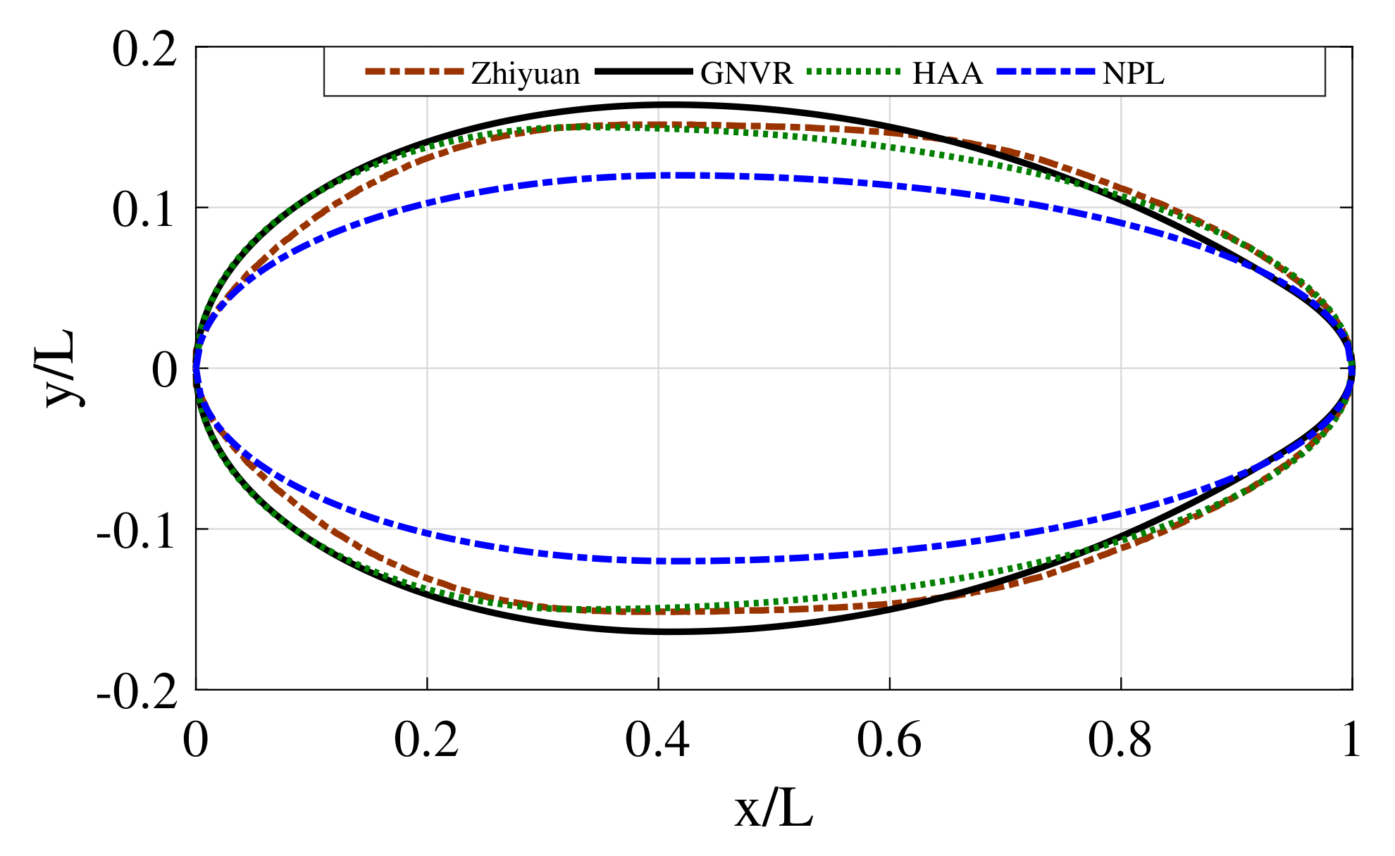
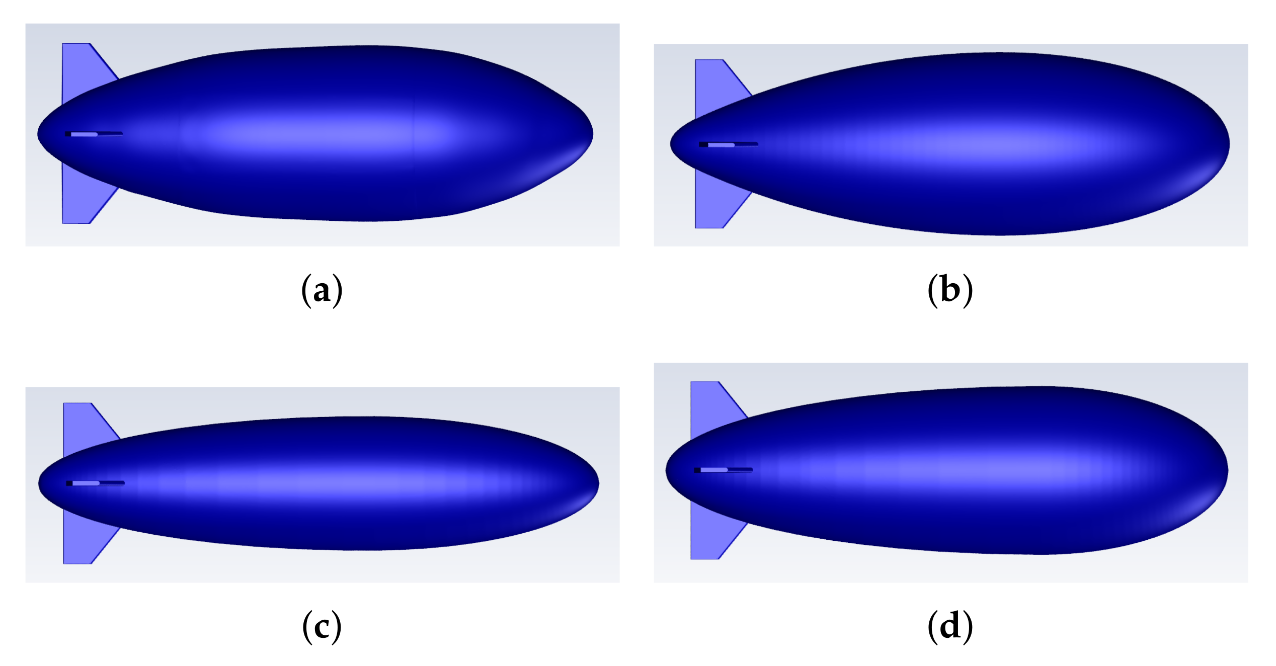
The stability derivatives involved in the rotational pitch motion (about the Y-axis) can be expressed as the linear decomposed forces and moment as follows:
D a p = D e + D ˙ α α + D ˙ α ˙ α ˙ + D ˙ q q + D ˙ q ˙ q ˙ L a p = L e + L ˙ α α + L ˙ α ˙ α ˙ + L ˙ q q + L ˙ q ˙ q ˙ M a p = M e + M ˙ α α + M ˙ α ˙ α ˙ + M ˙ q q + M ˙ q ˙ q ˙
A forced sinusoidal oscillatory motion will be induced on the aerostat pitch axis, as shown in Figure 1b. The oscillation is described in terms of the displacement α = ν = q a sin ω p t , velocity α ˙ = q = ω p q a cos ω p t and acceleration q ˙ = ω p 2 q a sin ω p t . Putting the values of w and w ˙ into Equation (11) gives
D a p = D e + D ˙ α q a sin ω p t + D ˙ α ˙ ω p q a cos ω p t + D ˙ q ω p q a cos ω p t D ˙ q ˙ ω p 2 q a sin ω p t L a p = L e + L ˙ α q 0 sin ω p t + L ˙ α ˙ ω p q a cos ω p t + L ˙ q ω p q a cos ω p t L ˙ q ˙ ω p 2 q a sin ω p t M a p = M e + M ˙ α q 0 sin ω p t + M ˙ α ˙ ω p q a cos ω p t + M ˙ q ω p q a cos ω p t M ˙ q ˙ ω p 2 q a sin ω p t
A comparison of the in-phase and out-of-phase values of Equations (6) and (12) gives
D ˙ α q 0 D ˙ q ˙ ω p 2 = a 2 ; D ˙ α ˙ + D ˙ q = a 1 / ( ω p q 0 ) L ˙ α q 0 L ˙ q ˙ ω p 2 = b 2 ; L ˙ α ˙ + L ˙ q = b 1 / ( ω p q 0 ) M ˙ α q 0 M ˙ q ˙ ω p 2 = c 2 ; M ˙ α ˙ + M ˙ q = c 1 / ( ω p q 0 )
By considering two pitch oscillating frequencies, ω p 1 and ω p 2 , the stability derivatives due to pitching accelerations can be calculated as
D ˙ q ˙ = a 2 ω p 2 a 2 ω p 1 q 0 ( ω p 1 2 ω p 2 2 ) L ˙ q ˙ = b 2 ω p 2 b 2 ω p 1 q 0 ( ω p 1 2 ω p 2 2 ) M ˙ q ˙ = c 2 ω p 2 c 2 ω p 1 q 0 ( ω p 1 2 ω p 2 2 )
According to Equations (13) and (14), a full-cycle response of drag, lift and moment for the forced oscillation about the pitch axis will give the six stability derivatives due to pitching velocity and acceleration.

3. Aerostat Shapes

In this study, a four-winged aerostat with a “+” orientation of the wings is considered. The length of the aerostat is fixed as 13.5 m by considering the required volume for the desired payload weight. Four different aerostat envelope shapes obtained from the open literature were considered for the comparison of stability derivative results obtained from the current study. They are the Zhiyuan shape [30], GNVR shape [39], NPL shape [39] and HAA shape [40], as shown in Figure 2. These shapes were selected by considering the variation of their leading-edge geometry, diameter and lift–drag characteristics, which will be shown in Section 5.5. It is possible to obtain the equation for the geometry of each aerostat, but in this work, the 2D coordinates of their profiles from the above-mentioned references were used. The 3D models used for the simulation analysis are shown in Figure 3. The maximum diameter is 2.025 m for the Zhiyuan shape, 2.212 m for the GNVR shape, 1.62 m for the NPL shape and 2.025 m for the HAA shape. Among the four aerostat shapes considered, Zhiyuan has the maximum volume and NPL has the least volume.

4. Numerical Simulation

4.1. Governing Equations

The current study involves the simulations performed using a commercial CFD solver, FLUENT 20.0. The 3D, incompressible, unsteady flow was solved with the help of the Reynolds Averaged Navier–Stokes (RANS) equations [43]. The governing equations can be expressed as
· V = 0 ρ V t + ρ · V V = p + · ( τ = ) + ρ g
where ρ is the density, V is the velocity, p is the pressure and g is the acceleration due to gravity. The stress tensor τ = can be expressed as
τ = = μ + μ t V + V T 2 3 · V I
where μ is the dynamic viscosity, μ t is the turbulence viscosity and I is an identity matrix.
The SIMPLE algorithm was utilized for the pressure velocity coupling, and the second-order upwind scheme was utilized for the spatial discretisation of the convective terms. A standard interpolation scheme was utilized for the pressure interpolation and an iterative time advancement scheme was used for time advancement. The convergence criterion was set to the order of 10 5 for velocity, continuity and turbulence quantities.

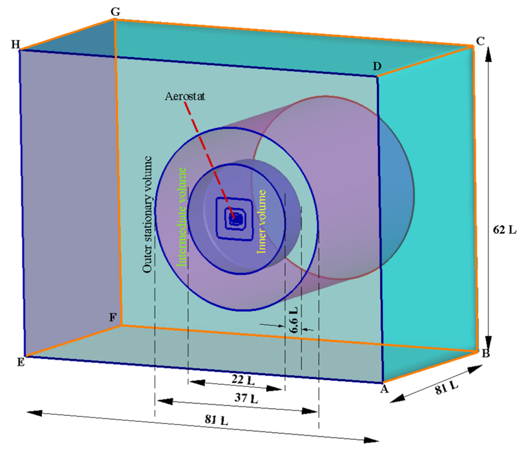
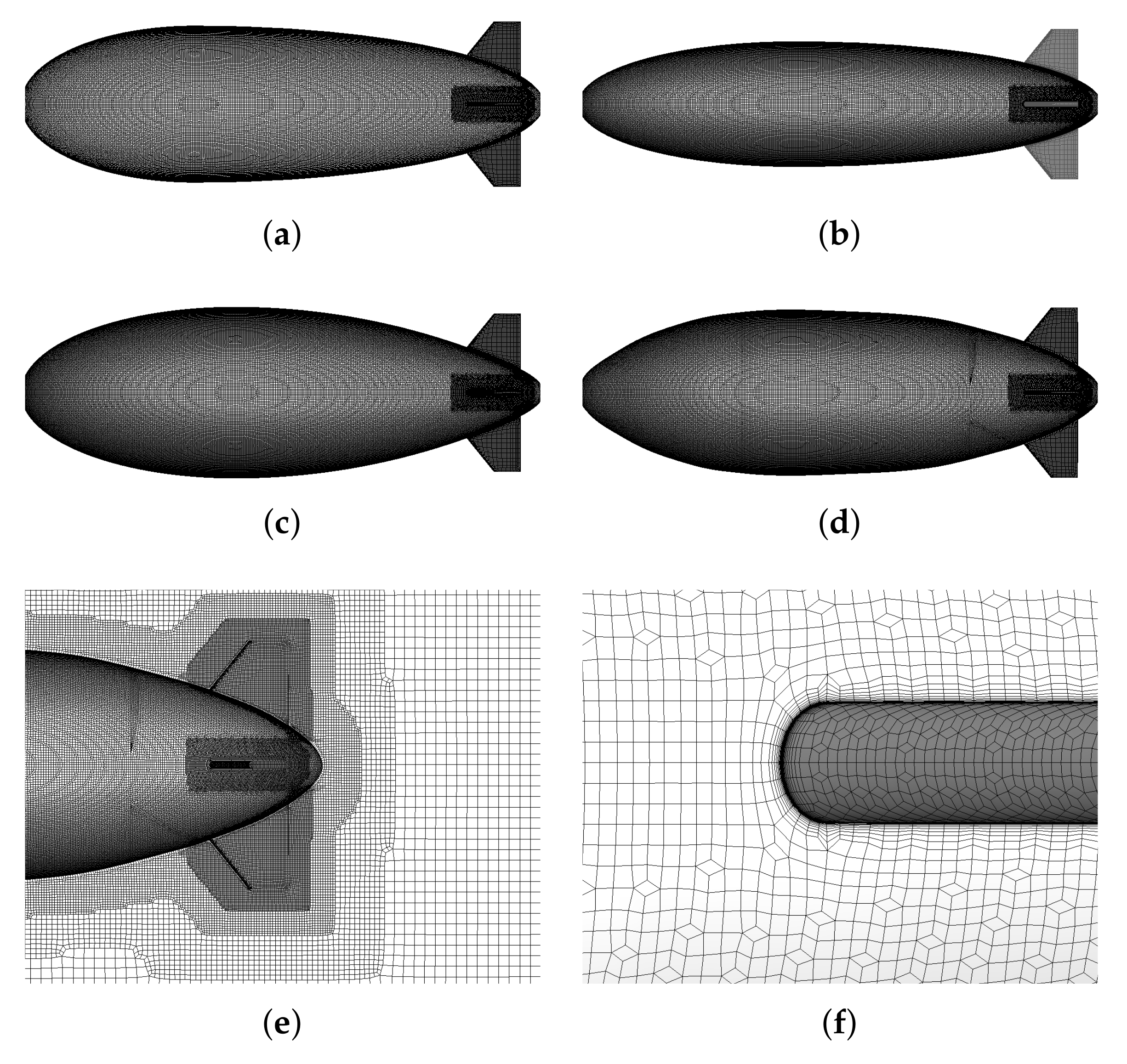
4.2. Computational Setup—Domain and Mesh

The domain for the computation considered for the current study is given in Figure 4. The dimensions for the domain were selected after an initial domain independence study. On each of the four faces of the outermost box volume depicted in Figure 4, there are four velocity inlets (faces ABCD, BCFG, CDHG and ABEF), symmetry on one face (face ADHE) and a pressure outlet on the other (face EFGH). All of the aerostat simulations in this paper used the same outer and intermediate volumes. The domain dimensions were determined by the length of the aerostat model. The heave and surge oscillation simulations were created using the dynamic mesh feature, while the pitching oscillation was created using the mesh motion feature. The inner and intermediate volumes were specified as rigid bodies, and the outer volume was kept stationary for the surge and heave motions. The inner volume was forced to move by the specified user-defined function, and the outer and intermediate volumes were kept stationary for the pitching motion simulation.
The computational grid used for the current study was made using GAMBIT and FLUENT meshing. The grid for outer and intermediate volumes (refer to Figure 4) was made using GAMBIT with a total of 0.1M tetrahedral–hexahedral hybrid cells. Comparatively, the coarse grid was used for the outer volumes. The grid for the inner volume with the aerostat (different for each aerostat shape) was made using ANSYS FLUENT meshing, as shown in Figure 5. The range of the number of cells used for each shape is 3 to 3.5 M. The cut cell mesh topology was used for the inner volumes. The proximity of the aerostat was finely meshed using a refining body of influence in the shape of an ellipse. The nearby volume (inner) mesh has 50 × 50 × 15 grid points on the X-axis, Y-axis and Z-axis. The viscous boundary layer was specified with 5 × 10 5 as its first layer’s thickness; 1.35 was chosen as the stretching ratio, and 18 layers were taken for the current aerostat surface. The average wall “Y+” value is 0.435 with a minimum of 0.0349 and a maximum of 1 for the above-mentioned mesh configuration.

4.3. Simulation Details

Each simulation included a steady-state simulation at the beginning, followed by a transient set of simulations without any motion. The transient simulation was run till appreciable convergence was obtained. Then, the sinusoidal input specified as a user-defined function was used for the dynamic simulation. Three frequencies were considered for the sinusoidal oscillations; 2.327 , 2.094 and 1.903 , corresponding to three time periods of 2.7 s, 3 s and 3.3 s. Five full cycles were simulated, and the last stable cycle was taken for the stability derivative extraction. A time interval of T s /800 s was adopted for the computational analysis. The details of the simulations performed for the current work are consolidated in Table 1. In the table, some of the amplitudes are velocities and some are angles. They are denoted by their corresponding units. Some of the validation studies were conducted using International Electrotechnical Commission (IEC) gust. The present study was conducted in the range of Reynolds numbers between 1.8 × 10 6 and 3.3 × 10 6 . The Mach number for the simulations considered in this paper was 0.02.

5. Simulation Results

The current section mainly discusses the simulation results for the stability derivative extraction study presented in Section 2. Results of some validation studies performed before the aerostat stability derivative extraction, such as the model validation, CFD mesh motion validation using NACA 0012 airfoil and stability derivative extraction for a prolate spheroid, are presented first. This is followed by the static aerodynamic data for the Zhiyuan aerostat, along with a comparison with the other three shapes. Then, the stability derivatives for the Zhiyuan aerostat are presented for different angles of attack. The results obtained for the Zhiyuan aerostat are compared with those for the other three aerostat shapes.

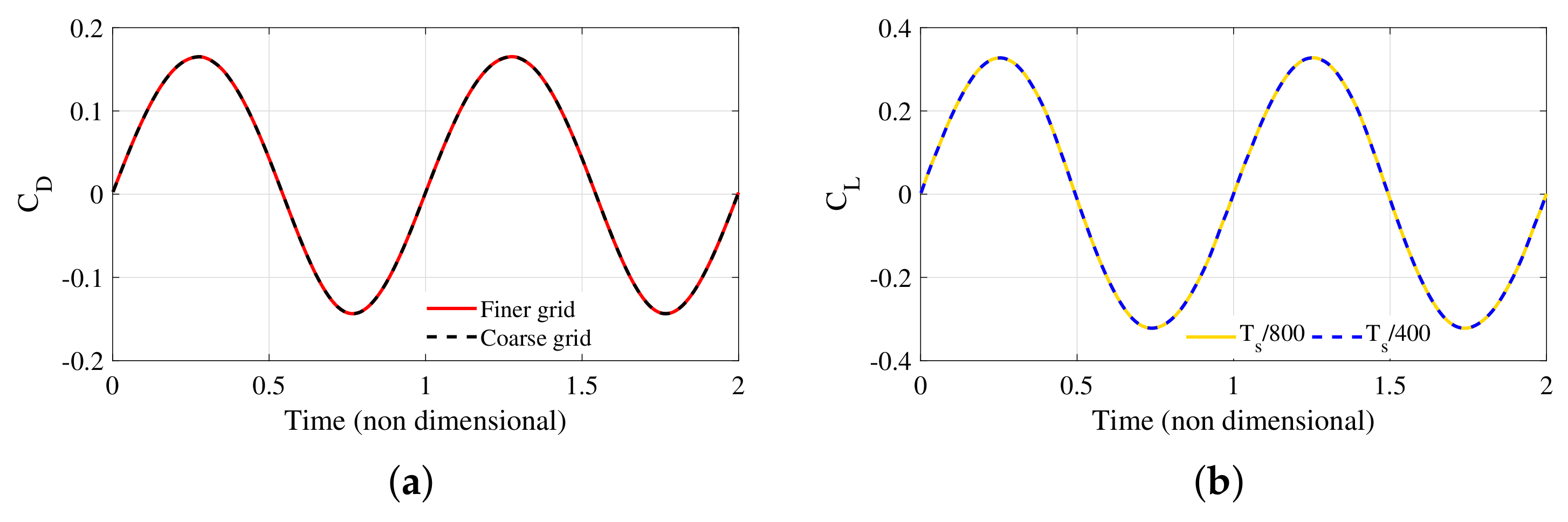
5.1. Grid and Time Step Independence Study

The efficacy of the mesh used for the analysis was tested for different grid refinements, as shown in Figure 6a, and the simulation time step independence study was performed, as shown in Figure 6b. The simulation was performed by providing the Zhiyuan aerostat with an unsteady velocity in the form of a sinusoidal gust, 0-degree angle of attack and a heave oscillation. The coefficients of drag and lift were measured respectively for the comparison. The results show that the grid used for the study is independent of the grid refinement and the time step.

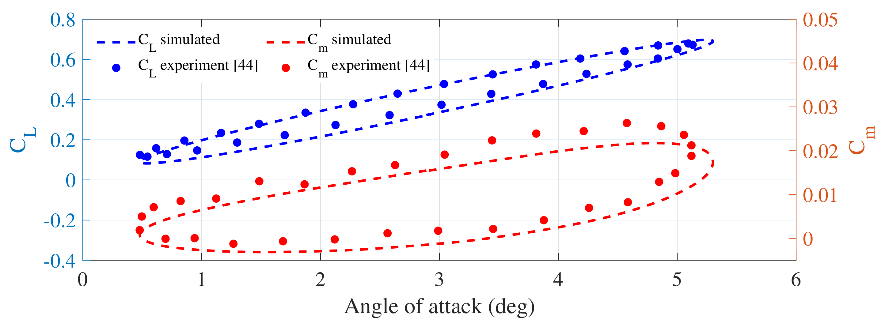
5.2. Validation of the Grid Motion

Validation of the dynamic mesh method, which was used for the linear oscillations of the current model, and the mesh motion feature used in the rotational motions of the model was performed with the help of the AGARD dataset [44]. NACA’s 0012 airfoil test data were considered for the analysis. As a result, a comparison of the lift and pitch coefficients with respect to the experimental results is shown in Figure 7. The closeness of the results validates the use of the methodology for further simulations.

5.3. Validation of the Stability Derivative Extraction Methodology

The methodology for the calculation of stability derivatives discussed in Section 2 was validated using the 6:1 prolate spheroid. The added mass coefficients were compared with the theoretical calculation, as well as with the simulation study by [30].
For the calculation of L ˙ w ˙ , a sinusoidal translational oscillation with an amplitude of 1 m/s and a frequency of 3.9 rad was considered. For the calculation of M ˙ q ˙ , two different sinusoidal oscillations having an amplitude of 5 deg and frequencies ω 1 = 29.79 rad and ω 2 = 21.06 rad were used.
The analytical calculations can be performed using the following formulations [45]:
L ˙ w ˙ = 4 3 π ρ a b c C 0 2 C 0
M ˙ q ˙ = 4 15 π ρ a b c ( a 2 c 2 ) 2 ( A 0 C 0 ) 2 ( c 2 a 2 ) + ( C 0 A 0 ) ( c 2 + a 2 )
The simulations resulted in the value of L ˙ w ˙ as 0.0457 , and the analytical result is 0.0430 ; for M ˙ q ˙ , the results are 0.00339 and 0.0033 , respectively.

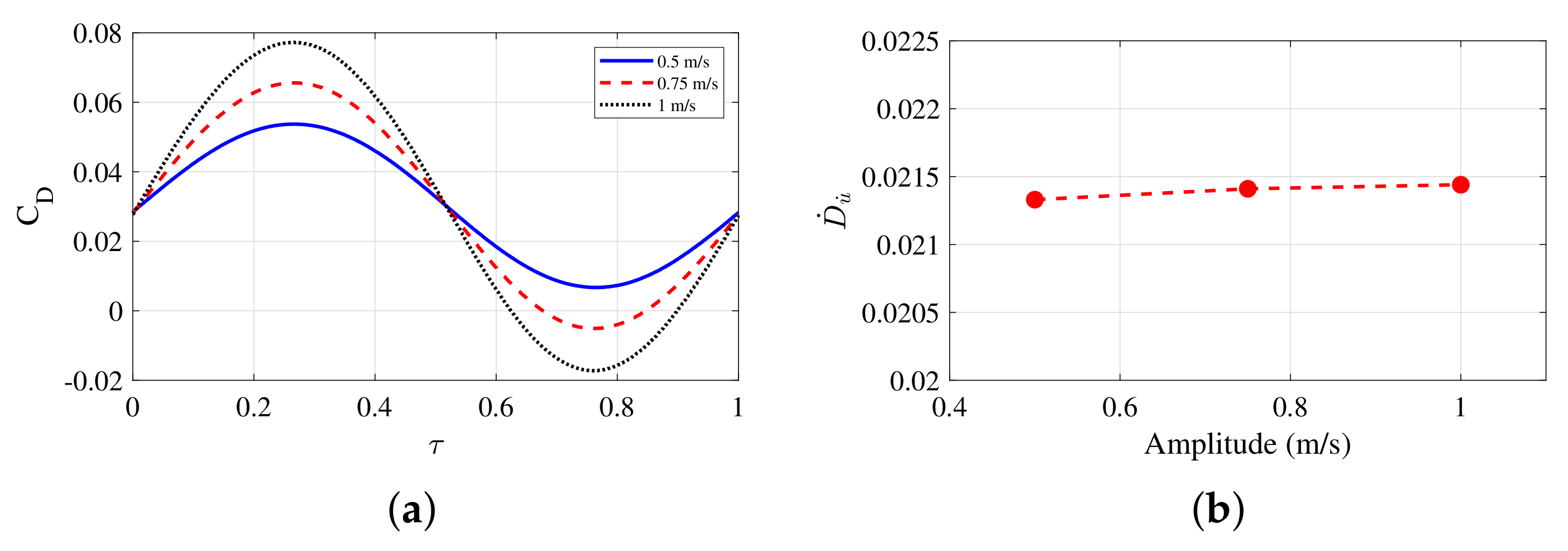
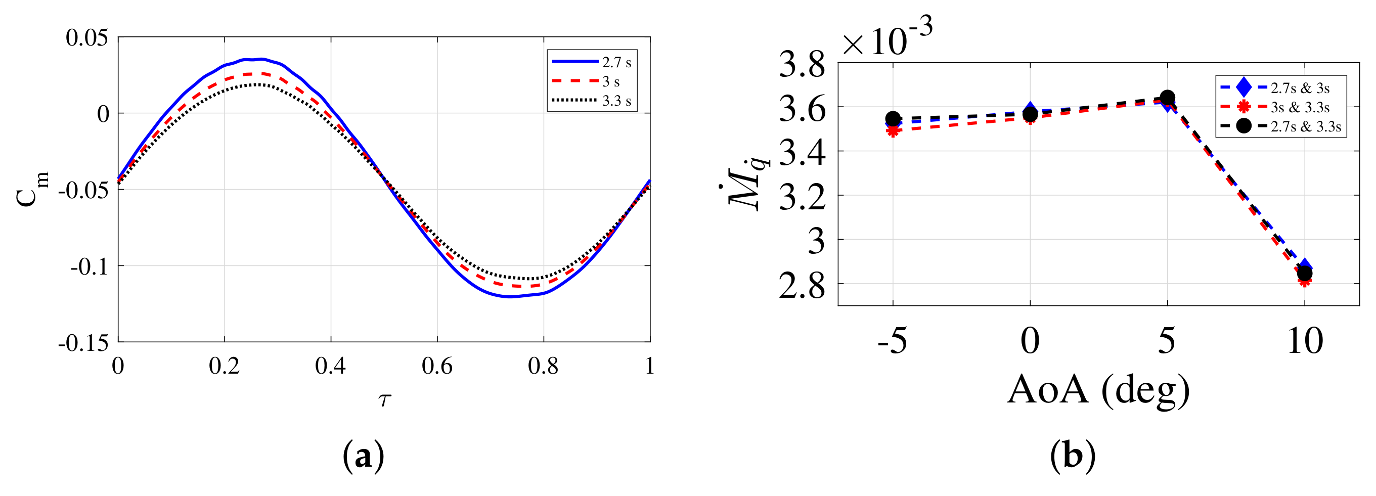
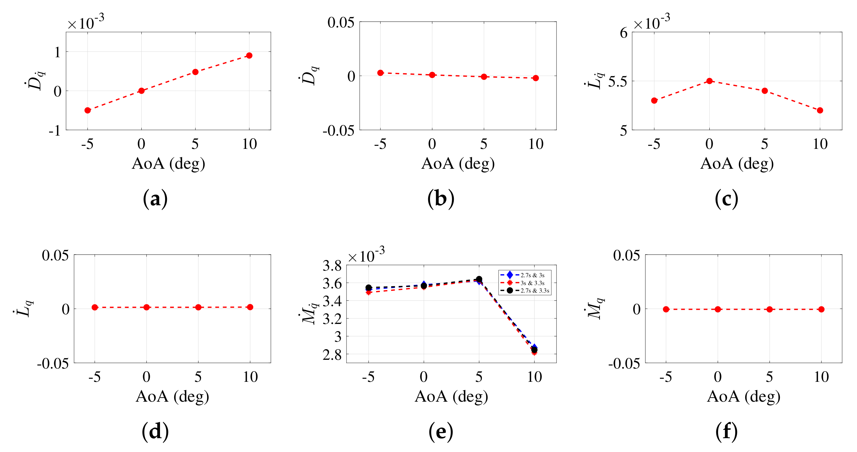
5.4. Acceleration and Frequency Independence Study

As the current study involves the forced oscillation of the aerostat along the three degrees of freedom, the independence study of the stability derivatives from the amplitude of oscillations (acceleration of the motion) has to be performed. Such a study was conducted for the Zhiyuan aerostat for surge, heave and pitch oscillations, and the acceleration independence was tested for all the stability derivatives involved. As a representative result, the acceleration independence study conducted for surge motion is shown in Figure 8. The coefficients with almost the same values show the simulation’s acceleration independence.
The estimation of moment stability derivatives involves the application of two sinusoidal oscillations with different frequencies. A frequency independence study was conducted for all the stability derivatives that required two frequencies. Figure 9 shows the results of the estimation of M ˙ q ˙ for a 10 0 angle of attack. Here, three frequencies were used for the comparison: 2.32 rad/s (2.7 s), 2.09 rad/s (3 s) and 1.90 rad/s (3.3 s). The frequency independence of the simulation is clearly observable in Figure 9.

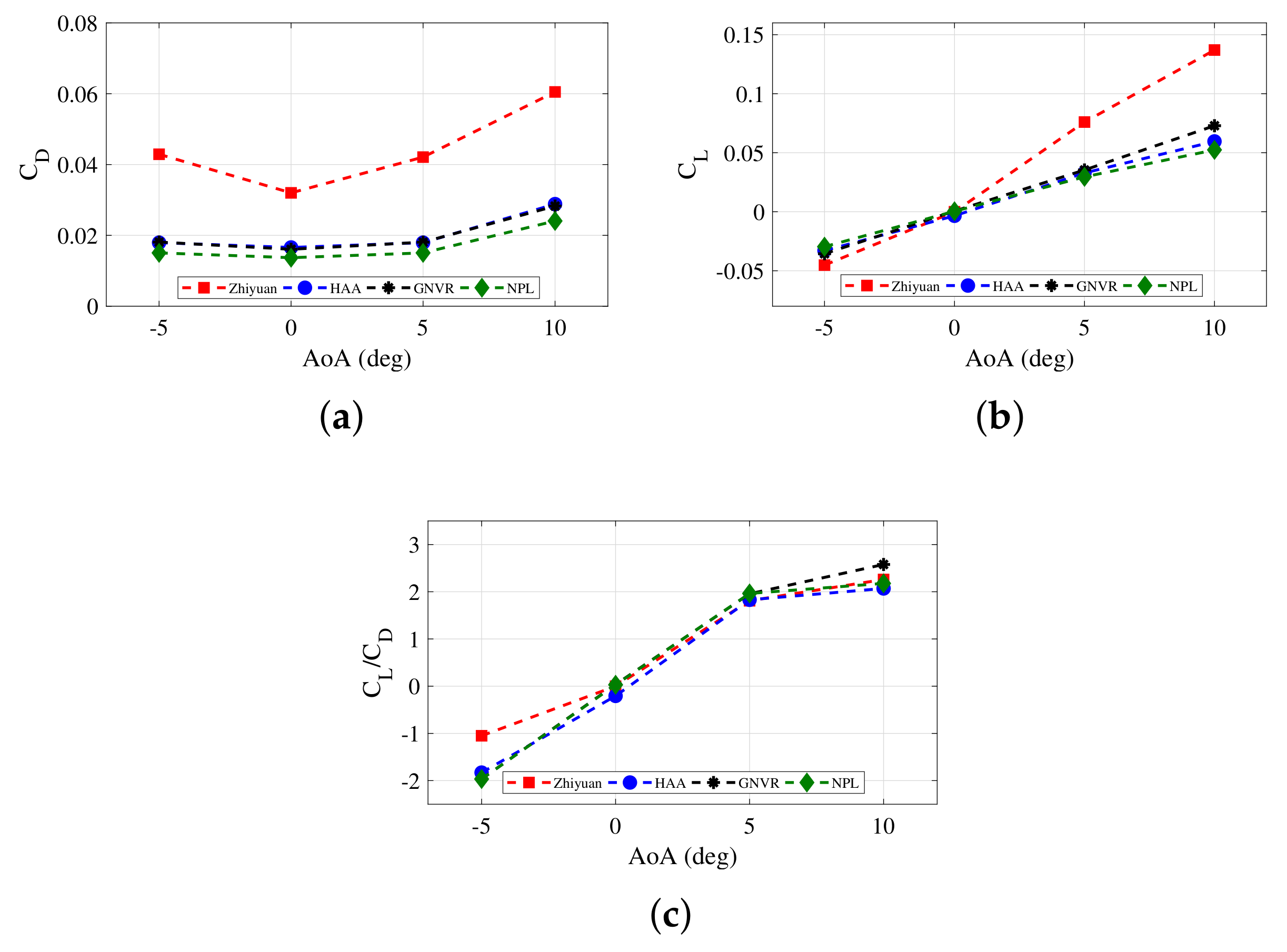
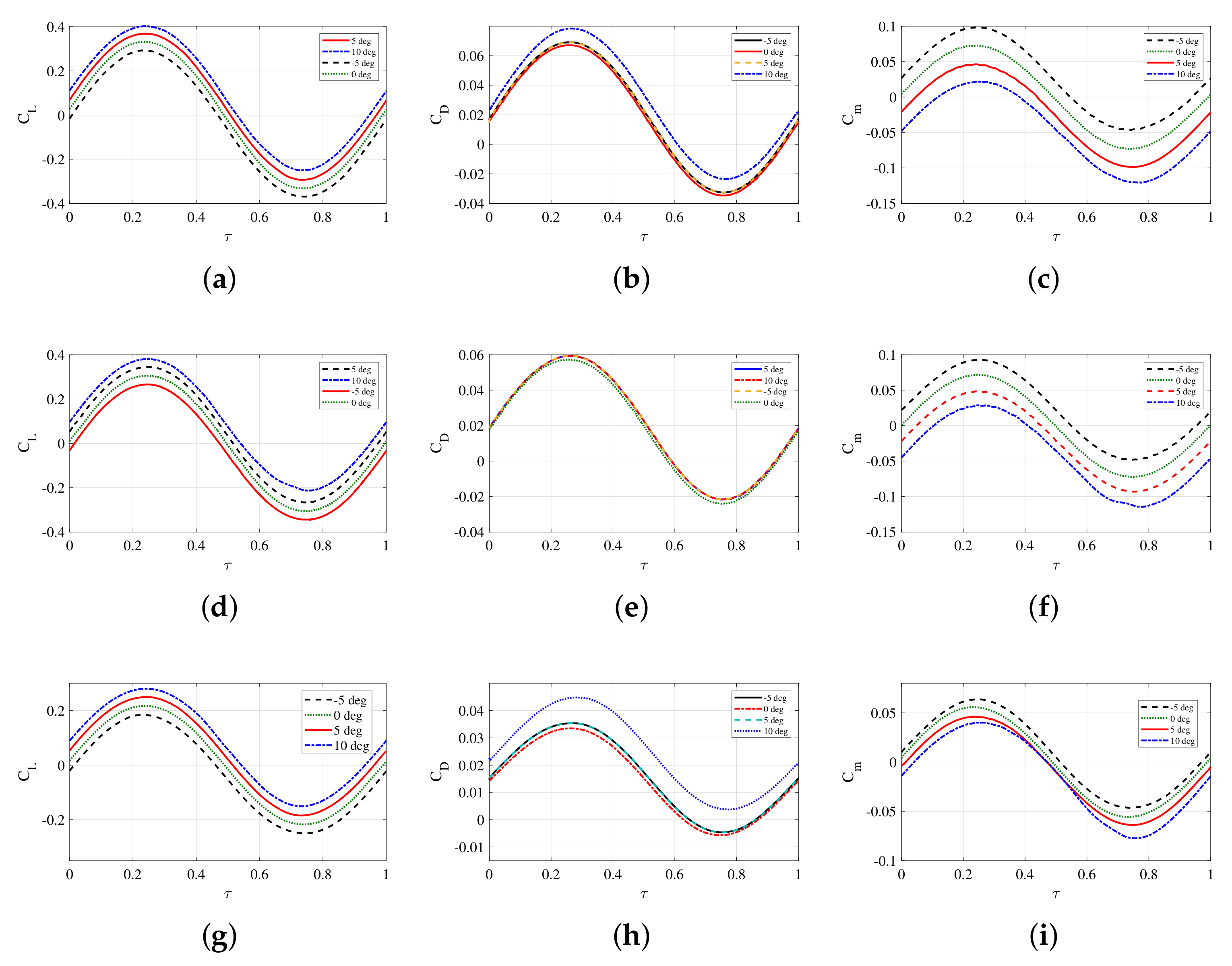
5.5. Static Aerodynamic Characteristics

Before proceeding with the dynamic stability derivatives’ extraction, the static aerodynamic characteristics of the Zhiyuan aerostat, along with the other three aerostats, were studied. This was done by conducting transient simulations with a steady velocity of 7.5 m/s for each aerostat. No oscillations were induced on the aerostat for the static derivative extraction simulations.
The coefficients of drag and lift forces were used for the analysis. Four different angles of attack were considered for this analysis. The angles of attack were selected based on the consideration that all the flight scenarios of the aerostat should be included [9].
A comparison of the drag and lift for the Zhiyuan base case and the other three aerostats for various angles of attack is given in Figure 10a,b. The symmetric nature of the variation of the forces with the angle of attack is clearly seen in the figure. The axisymmetric nature of the aerostat shapes causes these symmetric characteristics. The Zhiyuan shape shows the highest drag for all the angles of attack. This is due to the larger front area and the larger surface area of the shape among all four aerostat shapes. They contribute to the pressure, as well as the skin friction drag. As the angle of attack increases from zero, the area exposed to the free stream wind increases and aids the drag formation. The drag response for the other three aerostats is also shown in Figure 10a. All the other three aerostats also have similar drag characteristics with a reduced magnitude. The NPL shape has the least drag among the four aerostat shapes because of its least frontal area and surface area. The GNVR aerostat and HAA aerostat have the same drag characteristics. This is due to the similar leading edge geometry for those two aerostats. The Zhiyuan aerostat has a comparatively non-aerodynamic leading edge, as seen in Figure 3, which causes a higher drag response among the four aerostats.
As the aerodynamic lift is generated by the differential pressure distribution around the aerostat surfaces, it also shows variation with the angle of attack. The lift response of the Zhiyuan aerostat, along with the other three aerostats, is shown in Figure 10b. The Zhiyuan shape has the maximum lift among all four shapes. As the angle of attack increases, the lift magnitude increases vastly. The largest volume among the four aerostats causes the Zhiyuan aerostat to have the maximum differential pressure between the upper and lower surfaces and, thereby, the maximum lift. As seen for the drag response, the lift response is also similar for the other three aerostats. The NPL aerostat has the least lift magnitude, and the GNVR aerostat has the maximum lift among the three aerostats.
The primary criteria for selecting the shape for an aerostat are the reduced drag and maximum lift for a particular flight condition. A low-drag profile may result in a lower lift and vice versa. Therefore, the aerodynamic shape for the aerostats was selected based on the lift–drag ratio and not on the individual lift and drag information. Figure 10c shows the lift–drag ratio of the four aerostats for different angles of attack. It is seen that all four aerostats exhibit similar characteristics except for Zhiyuan at the negative angle of attack. This justifies the authors’ selection of these aerostat shapes for the analysis because the ultimate goal is to select a low-drag shape with maximum lift for the wind measurement application.

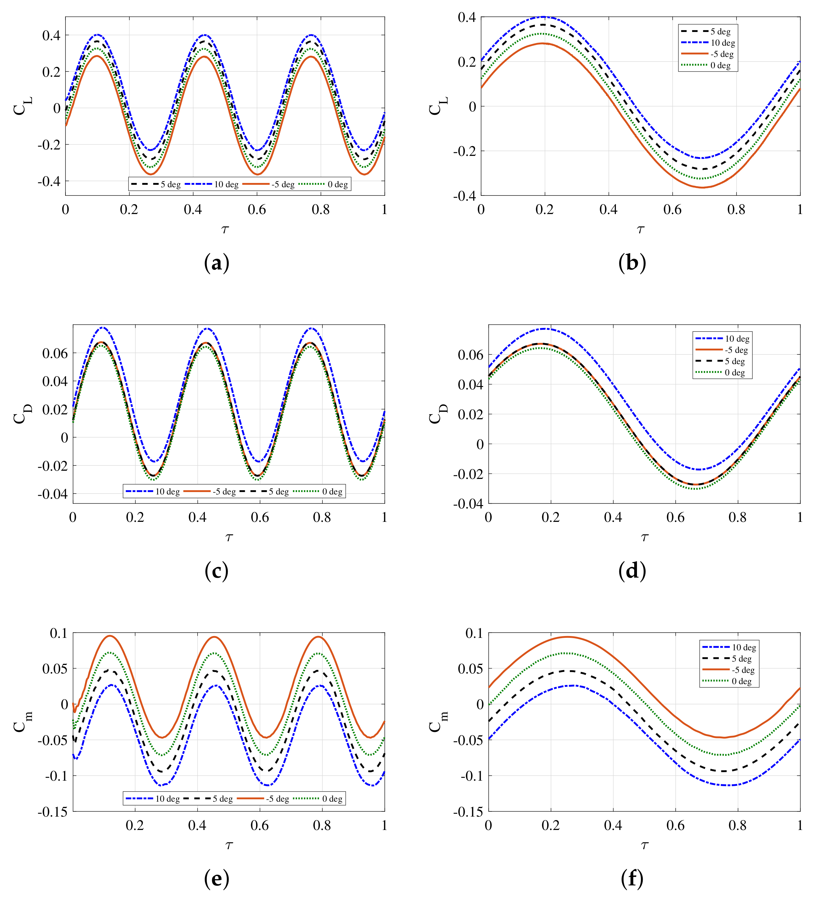
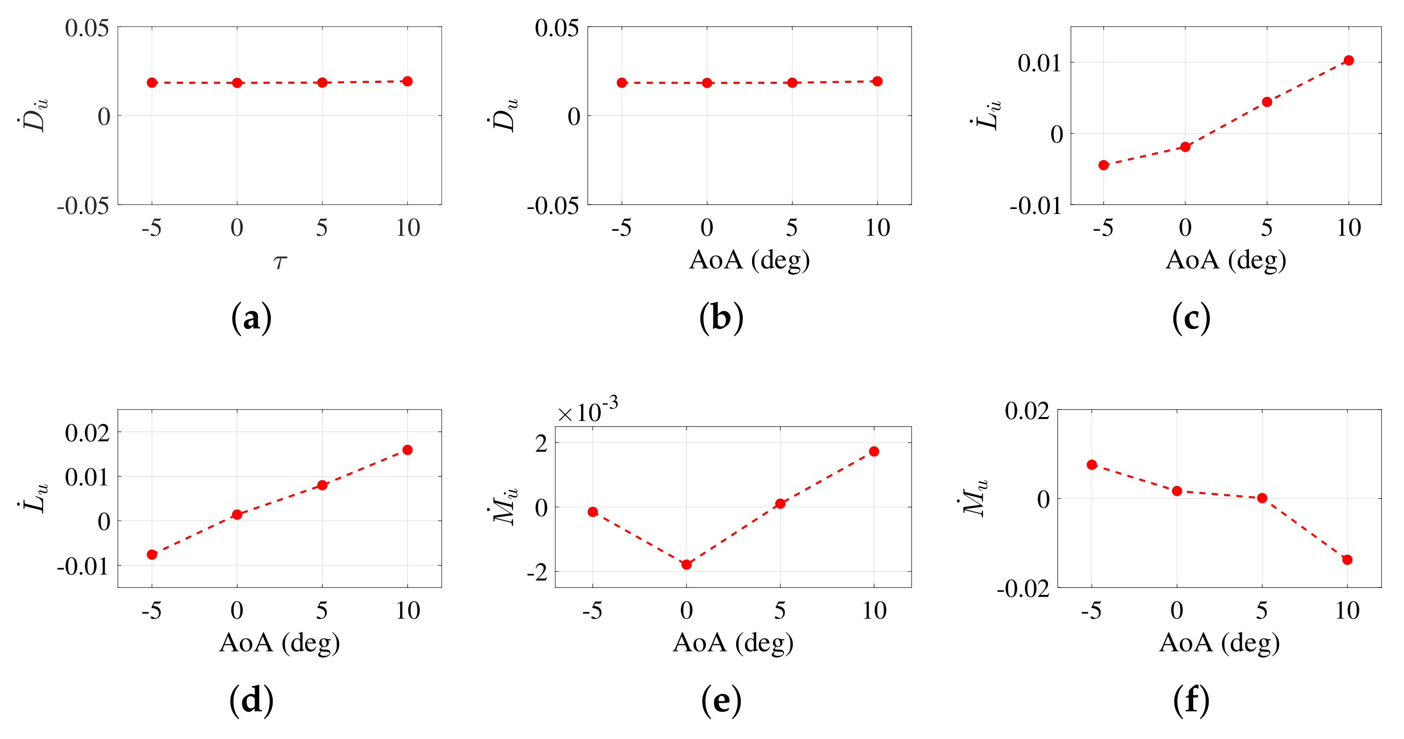
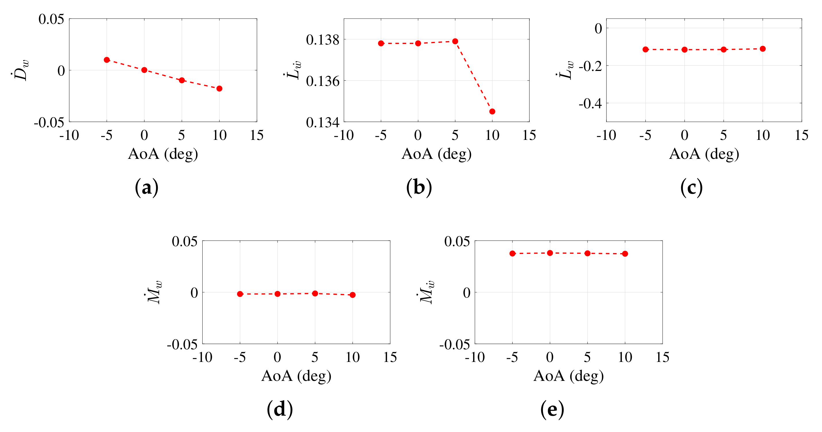
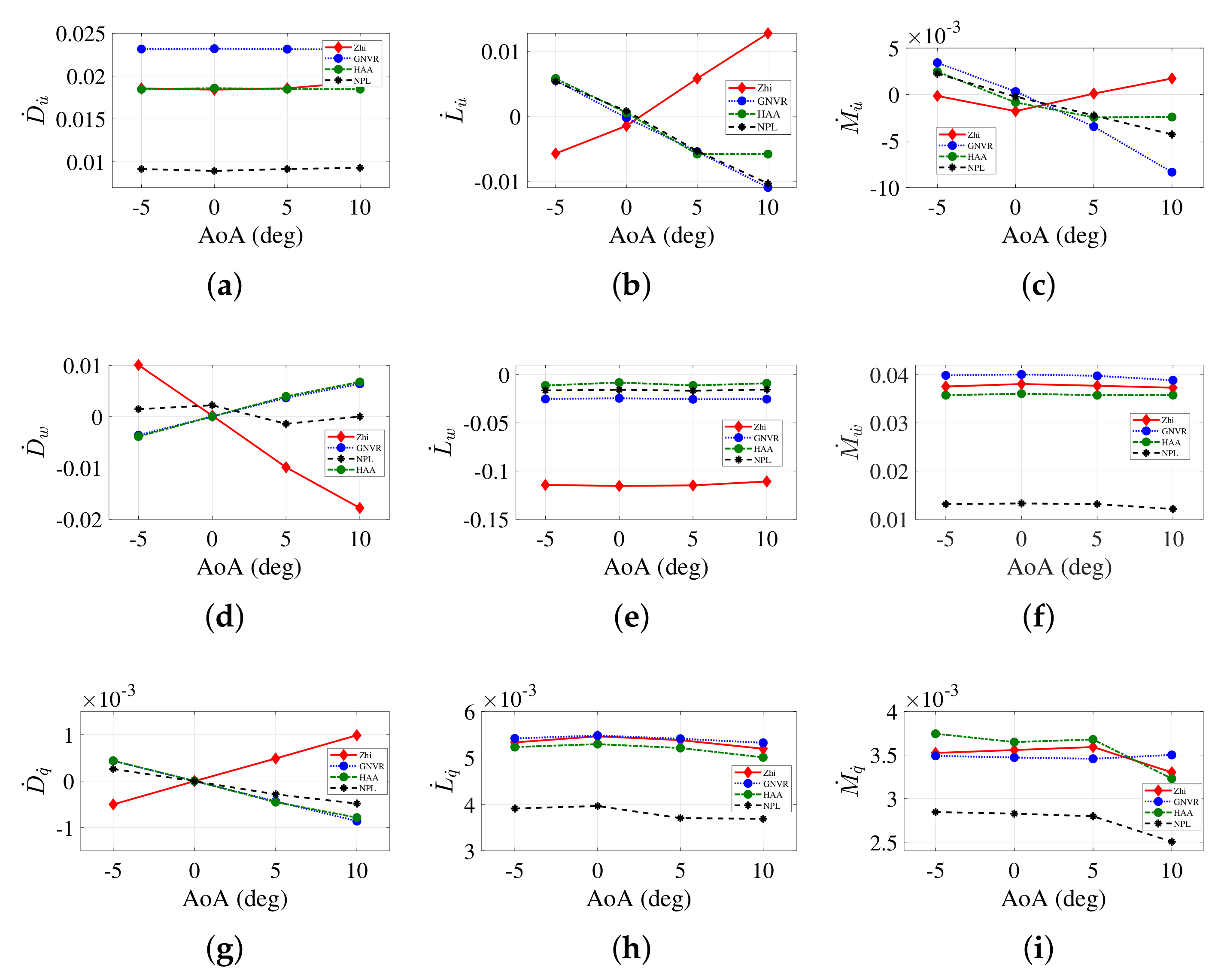
5.6. Dynamic Stability Derivatives

The dynamic stability derivative calculation methodology discussed in Section 2 was applied to the four aerostats with four different angles of attack. Three full cycles of responses were obtained for all the simulation cases, and a full stable cycle was selected for the analysis. The heave and surge oscillations were simulated using an amplitude of oscillation of 1 m/s and a frequency of oscillation of 2.09 rad. The pitch oscillations were simulated using an amplitude of oscillation of 5 deg and a frequency of oscillation of 2.09 rad, 2.32 rad and 1.9 rad. The drag, lift and moment response were measured for each aerostat shape for the heave, surge and pitch oscillations. All the responses are presented with non-dimensional time on the X-axis.

5.6.1. Zhiyuan Aerostat

The response of the Zhiyuan aerostat for heave oscillation, surge oscillation and pitch oscillation is shown in Figure 11. The figure shows the lift response for the heave oscillation, drag response for the surge oscillation and moment response for the pitch oscillation with a time period of 3 s. The first column of the figure represents a continuous set of responses, and the second column represents the single-cycle plots that are used for the stability derivatives’ extraction. As the input oscillations are sinusoidal, the responses are also sinusoidal, as shown in the figure.
As previously seen from the static aerodynamic response of the aerostat, the magnitude of lift increases with the increase in the angle of attack, as shown in Figure 11a. This is caused by a difference in differential pressure between the aerostat’s upper and lower surfaces. A further increase in the angle of attack may cause a stall condition, and this is not within the scope of the current study. The drag remains constant for the smaller angles of attack, as shown in Figure 11c, because the frontal area hit by the wind remains almost unchanged. The frontal area of the aerostat grows as the angle of attack rises towards 10 degrees and the drag rises. This is also seen from the static stability derivative shown in Figure 10a. The moment response shown in Figure 11 shows an inverse relation with the angle of attack. The moment reduces as the angle of attack increases and vice versa.
The stability derivatives of the Zhiyuan aerostat needed for the longitudinal dynamic model were extracted using the methodology specified in Section 2. A comparison of the stability derivatives calculated from the surge oscillations, heave oscillations and pitch oscillations for various angles of attack are given in Figure 12, Figure 13 and Figure 14, respectively.
The drag derivative due to the axial acceleration and axial velocity shown in Figure 12a,b, respectively, shows almost constant values for the small angle of attack. The derivative rises as the angle of attack approaches 10 degrees. This is in close agreement with the drag response shown in Figure 11a. The lift derivative due to the axial acceleration and velocity given in Figure 12c,d, respectively, shows a linear variation with the angle of attack. This shows the peculiar behavior of the aerostat to build up the lift as the axial acceleration happens, which aids the dynamic stability of the aerostat. The magnitude of the derivatives shifts from negative to positive as the angle of attack goes from negative to positive. At the 0 angle of attack, the derivative value is close to zero. That means the acceleration of the aerostat at a zero-degree angle of attack will not affect the lift much. The moment derivative due to the axial acceleration and axial velocity shown in Figure 12e,f, respectively, shows a linear decrease with the angle of attack. There is an exception at a 10 angle of attack for the acceleration derivative. Thus, the acceleration along the axial direction causes the moment to decrease, reducing the control effort for pitch control.
The drag derivative due to the vertical velocity, given in Figure 13a, linearly decreases with the angle of attack. In contrast, the lift derivative is almost constant, as shown in Figure 13c. The lift derivative due to vertical acceleration shown in Figure 13b remains constant for small angles of attack, but reduces to a lower value for the higher angle of attack. The vertical acceleration mainly caused by vertical gusts will not aid the drag buildup of the aerostat. On the other hand, it will not even benefit the lift generation of the aerostat. The moment derivative due to vertical velocity shows a variation opposite the moment derivative due to axial acceleration, as shown in Figure 13c. The moment derivative due to vertical acceleration remains constant for all angles of attack with the exception at zero degrees, as shown in Figure 13d.
The drag, lift and moment derivatives because of the pitching acceleration shown in Figure 14a,c,e, respectively, include the application of two different oscillations, as explained in Equation (14), with time periods of 2.7, 3 and 3.3 s. Three different sets of results are presented to check the effect of the selection of the second frequency for the calculation. The results show considerable similarity among the frequency pairs. For the remaining aerostat shapes, the oscillation frequencies for the pitching oscillations were taken as 2.7 s and 3 s. Due to the pitching velocity, the drag derivative shows a linear decrease with the angle of attack, whereas the lift derivative shows an increase with the angle of attack. The moment derivative because of the pitching velocity remains almost constant with the angle of attack variation. The pitching acceleration aids the lift generation and weakens the drag generation of the aerostat.

5.6.2. GNVR, HAA and NPL Aerostats

The simulations for extracting the stability derivatives for the longitudinal dynamic model of the considered aerostat by inducing axial (surge), vertical (heave) and pitch oscillations were repeated for the GNVR, HAA and NPL aerostats as well. Here, in this section, some of those results that showed a deviation from the Zhiyuan response are presented.
The response of the GNVR aerostat, HAA aerostat and NPL aerostat for heave oscillation, surge oscillation and pitch oscillation is shown in Figure 15. A stable cycle of response considered for the stability derivatives’ calculation is shown in the figure.
The lift response of the GNVR aerostat for various angles of attack shows an increment with the angle of attack, similar to the static stability derivatives, as shown in Figure 15a. The close similarity between the Zhiyuan shape and GNVR shape made the lift response of these two aerostats similar. The drag response of the GNVR aerostat shown in Figure 15b has a considerable deviation from that of the Zhiyuan aerostat. Due to the more streamlined design, the Zhiyuan aerostat has a reduced drag compared to the GNVR aerostat. The moment response of the GNVR aerostat shown in Figure 15c is similar to that of the Zhiyuan aerostat. The lift response of the HAA aerostat for various angles of attack is shown in Figure 15d. The amplitude of the lift increases with the increase in the angle of attack. The drag response shown in Figure 15e demonstrates an invariant relation with the angle of attack. The moment response, shown in Figure 15f, reduces with the rise in the angle of attack. The lift response of the NPL aerostat shown in Figure 15g shows the least lift magnitude for the given angles of attack, which is in close agreement with the static derivative response given in Figure 10b. The drag response remains constant for the smaller angles of attack and shows a minute increment in the magnitude for the 10-degree angle of attack, as shown in Figure 15h. The drag magnitude is also the least among the four aerostats, as seen from the static derivative results in Figure 10a. The moment response of the NPL aerostat, similar to the other three aerostats, shows an inverse relation with the angle of attack, as shown in Figure 15i.
The stability derivatives obtained for the Zhiyuan aerostat were compared with those for the other aerostats, as shown in Figure 16. The drag derivatives due to axial acceleration for the four aerostats shown in Figure 16a remain constant with the angle of attack. This is in agreement with the static aerodynamic characteristics shown in Figure 10a. Even though the individual derivatives remain constant, their magnitude varies largely among the aerostats. The GNVR aerostat has the maximum value, and the NPL has the minimum value, as shown in the figure. As seen for the Zhiyuan aerostat case in Figure 12a, the drag derivatives for the 10-degree angle of attack show a deviation for all the aerostats. This is due to the increase in the frontal area of the aerostat due to the large angle of attack. The magnitude of the drag derivative for the GNVR aerostat is slightly higher than that for the Zhiyuan aerostat. This can be explained by the slightly larger diameter of the GNVR aerostat, which causes the front area to increase slightly. In a similar way, the diameter of the NPL aerostat is smaller than the Zhiyuan aerostat, which causes the front area to be smaller than the other aerostat, thereby resulting in a smaller drag. This drag magnitude pattern is reflected in the rate of change of drag as well. As the diameter of the Zhiyuan and HAA aerostats were the same, the drag response and the drag derivative remained the same, as shown in the figure. The lower drag derivative value of the NPL aerostat helps to maintain the attitude of the aerostat because, as the aerostat accelerates forward, the drag buildup will be comparatively less among the four aerostats. On the other hand, the other three aerostats need more station-keeping control effort.
The lift derivative due to the axial acceleration for the four aerostats is shown in Figure 16b. There is a peculiar difference between the derivative response of the Zhiyuan aerostat among the other aerostats. As the angle of attack increases, the rate of change of lift due to the axial acceleration increases linearly, whereas the derivatives decrease for the other aerostats. This particular behavior of the Zhiyuan aerostat is advantageous for the dynamic stability of the aerostat as the increased lift helps the aerostat be more stable. The geometry of the Zhiyuan aerostat causes this particular response. All the other aerostats considered have a less pointy leading edge than the Zhiyuan aerostat. The positive slope in the lift derivative with the axial acceleration of the Zhiyuan aerostat aids the altitude control and station-keeping control efforts. The acceleration along the axial direction causes the lift to reduce its magnitude for the other three aerostats, unlike the Zhiyuan aerostat case. It shows that the aerostat fails to retain its lift as its own. There should be control actions to maintain the required lift for the aerostat.
The moment derivatives due to the axial acceleration for the four aerostats are shown in Figure 16c. The rate of change of moment decreases with the angle of attack for the other three aerostats. The reduction in the moment derivative due to the axial acceleration will reduce the control effort for the pitch control. The Zhiyuan aerostat moment derivative increases for the positive angle of attack, as shown in the figure. Thus, the Zhiyuan aerostat demands more control effort for maintaining the desired pitch for large positive angles of attack. Even though the stalling of the aerostat is not in the scope of this work, the pattern in the moment derivative for the Zhiyuan aerostat suggests that stalling occurs at a lower angle of attack than for the other three aerostats.
The drag derivatives due to the vertical velocity for the four aerostats are shown in Figure 16d. There is a positive slope for the derivatives plot for the GNVR, HAA and NPL aerostats and a negative slope for the Zhiyuan aerostat. Unlike the Zhiyuan aerostat, the drag magnitude builds up as the other three aerostats accelerate in the vertical direction, primarily due to vertical wind gusts. This demands more control effort for the station-keeping and attitude control for the aerostats. This shows that as the turning of the aerostat for a pitch-up flight occurs, such as taking off from the ground station, extra drag build-up causes the aerostat to slow down. The negative slope of the Zhiyuan aerostat aids the control efforts to maintain the position of the aerostat.
The lift derivatives due to the vertical velocity for the four aerostats shown in Figure 16e possess constant values for different angles of attack. The vertical acceleration can be due to the presence of a strong vertical wind gust or an ascending flight phase at the time of the installation or maintenance of the aerostat. The Zhiyuan aerostat has the maximum lift derivative in the negative direction, which demands more control effort for the station-keeping. All the other aerostats aid the lift for the ascending phase, which helps to reduce the control effort. The moment derivatives due to the vertical acceleration for the four aerostats shown in Figure 16f also remain constant for different angles of attack. The Zhiyuan, HAA and GNVR aerostats have the maximum value among the four aerostats, making the pitch control rapid and requiring more effort to keep them in the desired pitch. The NPL aerostat has the minimum value, which helps the aerostat vary the pitch smoothly with less control effort. The force and moment derivatives due to the pitch acceleration for the four aerostats are shown in Figure 16g–i. The drag derivative varies linearly with the angle of attack with a negative slope, whereas the Zhiyuan aerostat has a positive slope. The lift derivative shows an almost constant value for various angles of attack, with the NPL aerostat having the minimum value. The moment and lift derivatives are similar to the Zhiyuan aerostat except for the NPL aerostat.

6. Conclusions of the Study

This paper investigated the aerodynamic modeling of the aerostat using a CFD-based method. The intended application of the aerostat was to use it as a low-altitude wind measurement system. The presented study considered the translational motion of the aerostat in the X (surge) and Z (heave) directions and the rotational motion about the Y-axis (pitching). A small-amplitude sinusoidal oscillation was considered for the simulation of the aerostat motion. A methodology for the calculation of stability derivatives from the full-cycle oscillation responses of the aerostat was presented with CFD simulation results. A base case aerostat shape was selected for the analysis, and three other aerostat shapes were considered for the comparison of the results obtained from the analysis.
The translational oscillatory motion of the aerostat model was simulated using the dynamic mesh motion feature and the zone motion feature available with ANSYS FLUENT. The validation of the dynamic mesh motion method was performed using the NACA 0012 airfoil test data. The validation of the methodology considered for the stability derivatives calculation was performed using prolate spheroid test data. The experimental stability derivatives of the spheroid are available in the open literature. The results showed promising similarity with the theoretical calculations as well. The independence of the results on the amplitude and frequency of oscillations was tested successfully as well.
The static stability derivatives or static aerodynamic coefficients of the four aerostats were presented before the stability derivatives’ extraction. The Zhiyuan shape showed the maximum drag among the four shapes because of its large surface area and large front area. Being the shape with the least surface area, the NPL shape possessed the least drag. The lift characteristics of the Zhiyuan shape were better than all the other shapes due to its large surface area, which contributes to the differential pressure distribution. The lift–drag ratio of the aerostats showed that the Zhiyuan aerostat has the best static aerodynamic characteristics among the four aerostats.
The stability analysis and the control system design for the aerostat can be made better by considering the dynamic stability derivatives involving the small-amplitude motions of the aerostat. In this paper, the dynamic stability derivatives of the Zhiyuan aerostat at four angles of attack were presented, the results of which were compared with the derivatives of the other three aerostats as well. The drag and lift performance of the Zhiyuan aerostat is superior among the four aerostats. This will help the aerostat be controlled with less control effort during the station-keeping and attitude control tasks. The NPL aerostat had better moment stability for the pitching acceleration. This will make the Zhiyuan aerostat demand more control effort for the pitching maneuver.
From this study, it can be concluded that the Zhiyuan aerostat can be used for low-altitude wind measurement applications. The more aerodynamic geometry of the Zhiyuan aerostat compared to the other three aerostats was the main reason for this peculiar performance. The static lift–drag performance of the Zhiyuan aerostat was better among the four aerostats presented. The dynamic stability analyzed using the stability derivatives also suggests the superiority of the Zhiyuan aerostat among the four aerostats. The drag and lift performance of the Zhiyuan aerostat was such that it aided the station-keeping and attitude control efforts. Even though the moment stability was slightly below the NPL aerostat, the Zhiyuan aerostat can be operated for the pitching maneuver with some added control effort.
This study will be extended for the investigation of the control systems required for the station keeping of the aerostat at the desired attitude for wind measurement. The longitudinal stability derivatives can be extracted from the aerostat oscillations involving the longitudinal motion variables and can be used for the longitudinal dynamic model of the aerostat. An optimization of the aerostat geometry for improving the dynamic stability can be considered as a future direction of this study.

Author Contributions

Conceptualization, A.S., R.K.V. and V.R.M.O.; methodology, A.S. and R.K.V.; software, A.S., R.K.V. and A.M.; validation, A.S., R.K.V., S.J. and V.R.M.O.; formal analysis, A.S. and R.K.V.; investigation, A.S. and R.K.V.; resources, R.K.V., V.R.M.O. and A.M.; data curation, A.S., R.K.V., S.J., A.M. and V.R.M.O.; writing—original draft preparation, A.S. and R.K.V.; writing—review and editing, A.S., R.K.V., S.J., A.M. and V.R.M.O.; visualization, A.S. and R.K.V.; supervision, R.K.V. and V.R.M.O. All authors have read and agreed to the published version of the manuscript.

Funding

This research received no external funding.

Institutional Review Board Statement

Not applicable.

Informed Consent Statement

Not applicable.

Data Availability Statement

Not applicable.

Acknowledgments

A part of the computations was performed on the Aziz Supercomputer at King Abdulaziz University’s High-Performance Computing Center (http://hpc.kau.edu.sa/) (last accessed on 15 February 2022). The authors acknowledge the computer time and technical support provided by the center.

Conflicts of Interest

The authors declare no conflict of interest.

References

  1. Allison, S.; Bai, H.; Jayaraman, B. Wind estimation using quadcopter motion: A machine learning approach. Aerosp. Sci. Technol. 2020, 98, 105699. [Google Scholar] [CrossRef] [Green Version]
  2. Beaucage, P.; Lafrance, G.; Lafrance, J.; Choisnard, J.; Bernier, M. Synthetic aperture radar satellite data for offshore wind assessment: A strategic sampling approach. J. Wind Eng. Ind. Aerodyn. 2011, 99, 27–36. [Google Scholar] [CrossRef]
  3. Schmitt, N.P.; Rehm, W.; Pistner, T.; Zeller, P.; Diehl, H.; Navé, P. The AWIATOR airborne LIDAR turbulence sensor. Aerosp. Sci. Technol. 2007, 11, 546–552. [Google Scholar] [CrossRef]
  4. Grillo, C.; Montano, F. Wind component estimation for UAS flying in turbulent air. Aerosp. Sci. Technol. 2019, 93, 105317. [Google Scholar] [CrossRef]
  5. Anoop, S.; Velamati, R.K.; Oruganti, V.R.M.; Mohammad, A. Computational analysis of the aerodynamic characteristics and stability derivatives of an aerostat under unsteady wind conditions. J. Braz. Soc. Mech. Sci. Eng. 2022, 44, 225. [Google Scholar] [CrossRef]
  6. Satapathy, J.; Bhat, G.S. Studies of Extreme Gust Storm Events in Bengaluru, India. Curr. Sci. 2020, 119, 343–351. [Google Scholar] [CrossRef]
  7. Santos, L.; Marques, F. Nonlinear aeroelastic analysis of airfoil section under stall flutter oscillations and gust loads. J. Fluids Struct. 2021, 102, 103250. [Google Scholar] [CrossRef]
  8. Akhlaghi, H.; Soltani, M.R.; Maghrebi, M.J. Transitional boundary layer study over an airfoil in combined pitch-plunge motions. Aerosp. Sci. Technol. 2020, 98, 105694. [Google Scholar] [CrossRef]
  9. Anoop, S.; Velamati, R.K.; Oruganti, V.R.M. Aerodynamic characteristics of an aerostat under unsteady wind gust conditions. Aerosp. Sci. Technol. 2021, 113, 106684. [Google Scholar] [CrossRef]
  10. Mueller, J.; Paluszek, M.; Zhao, Y. Development of an Aerodynamic Model and Control Law Design for a High Altitude Airship. In Proceedings of the AIAA 3rd “Unmanned Unlimited” Technical Conference, Workshop and Exhibit, Chicago, IL, USA, 20–23 September 2004. [Google Scholar] [CrossRef] [Green Version]
  11. Jones, S.P.; DeLaurier, J.D. Aerodynamic estimation techniques for aerostats and airships. J. Aircr. 1983, 20, 120–126. [Google Scholar] [CrossRef]
  12. Ashraf, M.; Choudhry, M. Dynamic modeling of the airship with Matlab using geometrical aerodynamic parameters. Aerosp. Sci. Technol. 2013, 25, 56–64. [Google Scholar] [CrossRef]
  13. Anoop, S.; Oruganti, V.R.M. Modelling and simulation of aerodynamic parameters of an airship. Adv. Sci. Technol. Eng. Syst. J. 2020, 5, 167–176. [Google Scholar] [CrossRef]
  14. Mahmood, K.; Ismail, N.A. Application of multibody simulation tool for dynamical analysis of tethered aerostat. J. King Saud Univ. Eng. Sci. 2020, 34, 209–216. [Google Scholar] [CrossRef]
  15. Anoop, S.; Ramana Murthy, O.V.; Sharma, K.R. Analysis of Airship Dynamics using Linear Quadratic Regulator Controller. In Proceedings of the 15th IEEE India Council International Conference (INDICON), Coimbatore, India, 16–18 December 2018; pp. 1–6. [Google Scholar] [CrossRef]
  16. Zhao, L.; Liu, S.; Yan, J.; Ge, Y. Aerodynamic modeling for streamlined box girders using nonlinear differential equations and validation in actively generated turbulence. Wind Struct. Int. J. 2021, 33, 71–86. [Google Scholar] [CrossRef]
  17. Nguyen, K.; Au, L.T.K.; Phan, H.V.; Park, H.C. Comparative dynamic flight stability of insect-inspired flapping-wing micro air vehicles in hover: Longitudinal and lateral motions. Aerosp. Sci. Technol. 2021, 119, 107085. [Google Scholar] [CrossRef]
  18. Bykerk, T.; Verstraete, D.; Steelant, J. Low speed lateral-directional aerodynamic and static stability analysis of a hypersonic waverider. Aerosp. Sci. Technol. 2020, 98, 105709. [Google Scholar] [CrossRef]
  19. Bryan, G. Stability in Aviation: An Introduction to Dynamical Stability as Applied to the Motions of Aeroplanes; Macmillan and Company, Limited: New York, NY, USA, 1911. [Google Scholar]
  20. Mi, B.G.; Zhan, H. Review of Numerical Simulations on Aircraft Dynamic Stability Derivatives. Arch. Comput. Methods Eng. 2019, 27, 1515–1544. [Google Scholar] [CrossRef]
  21. Khoury, G. Airship Technology; Cambridge University Press: Cambridge, UK, 2012. [Google Scholar]
  22. Wu, Y.; Li, L.; Su, X.; Gao, B. Dynamics modeling and trajectory optimization for unmanned aerial-aquatic vehicle diving into the water. Aerosp. Sci. Technol. 2019, 89, 220–229. [Google Scholar] [CrossRef]
  23. Bykerk, T.; Verstraete, D.; Steelant, J. Low speed longitudinal dynamic stability analysis of a hypersonic waverider using unsteady Reynolds averaged Navier Stokes forced oscillation simulations. Aerosp. Sci. Technol. 2020, 103, 105883. [Google Scholar] [CrossRef]
  24. Badesha, S. Aerodynamics of the TCOM 71M aerostat. In Proceedings of the 10th Lighter-Than-Air Systems Technology Conference, Scottsdale, AZ, USA, 14–16 September 1993; pp. 1–4. [Google Scholar] [CrossRef]
  25. Ignatyev, D.I.; Khrabrov, A.N. Neural network modeling of unsteady aerodynamic characteristics at high angles of attack. Aerosp. Sci. Technol. 2015, 41, 106–115. [Google Scholar] [CrossRef]
  26. Waqar, A.; Ali, O.A.; Erwin, S.; Mohamed, A.J. Wind tunnel testing of hybrid buoyant aerial vehicle. Aircr. Eng. Aerosp. Technol. 2017, 89, 174–180. [Google Scholar] [CrossRef] [Green Version]
  27. Tao, Q.; Tan, T.J.; Cha, J.; Yuan, Y.; Zhang, F. Modeling and Control of Swing Oscillation of Underactuated Indoor Miniature Autonomous Blimps. Unmanned Syst. 2021, 9, 73–86. [Google Scholar] [CrossRef]
  28. Junior, J.L.M.; Santos, J.S.; Morales, M.A.; Goes, L.C.; Stevanovic, S.; Santana, R.A. Airship Aerodynamic Coefficients Estimation Based on Computational Method for Preliminary Design. In Proceedings of the AIAA Aviation Forum, Dallas, TX, USA, 17–21 June 2019. [Google Scholar] [CrossRef]
  29. Ullah, A.; Badar Zaman, M.; Aashan Bhatti, M.; Qasim, D.; Hamid, A.; Xiong, Q.; Khan, A. CFD study of drag and lift coefficients of non-spherical particles. J. King Saud. Univ. Eng. Sci. 2021, in press. [Google Scholar] [CrossRef]
  30. Wang, X.L. Computational Fluid Dynamics Predictions of Stability Derivatives for Airship. J. Aircr. 2012, 49, 933–940. [Google Scholar] [CrossRef]
  31. Ronch, A.D.; Vallespin, D.; Ghoreyshi, M.; Badcock, K.J. Evaluation of Dynamic Derivatives Using Computational Fluid Dynamics. AIAA J. 2012, 50, 470–484. [Google Scholar] [CrossRef]
  32. Ronch, A.D. On the Calculation of Dynamic Derivatives Using Computational Fluid Dynamics. Ph.D. Thesis, University of Liverpool, Liverpool, UK, 2012. [Google Scholar]
  33. Carrión, M.; Biava, M.; Barakos, G.N.; Stewart, D. Study of Hybrid Air Vehicle Stability Using Computational Fluid Dynamics. J. Aircr. 2017, 54, 1328–1339. [Google Scholar] [CrossRef] [Green Version]
  34. Lee, S.K.; Joung, T.H.; Cheo, S.J.; Jang, T.S.; Lee, J.H. Evaluation of the added mass for a spheroid-type unmanned underwater vehicle by vertical planar motion mechanism test. Int. J. Nav. Archit. Ocean Eng. 2011, 3, 174–180. [Google Scholar] [CrossRef]
  35. Mader, C.A.; Martins, J.R.R.A. Computing Stability Derivatives and Their Gradients for Aerodynamic Shape Optimization. AIAA J. 2014, 52, 2533–2546. [Google Scholar] [CrossRef] [Green Version]
  36. Muller, L.; Libsig, M.; Martinez, B.; Bastide, M.; Bidino, D.; Yannick, B.; Roy, J.C. Wind tunnel measurements of the dynamic stability derivatives of a fin-stabilized projectile by means of a 3-axis freely rotating test bench. In Proceedings of the AIAA Aviation Forum, Virtual, 15–19 June 2020. [Google Scholar] [CrossRef]
  37. Javanmard, E.; Mansoorzadeh, S.; Mehr, J.A. A new CFD method for determination of translational added mass coefficients of an underwater vehicle. Ocean Eng. 2020, 215, 107857. [Google Scholar] [CrossRef]
  38. Ghoreyshi, M.; Jirásek, A.; Cummings, R.M. Reduced order unsteady aerodynamic modeling for stability and control analysis using computational fluid dynamics. Prog. Aerosp. Sci. 2014, 71, 167–217. [Google Scholar] [CrossRef] [Green Version]
  39. Kale, S.; Joshi, P.; Pant, R. A generic methodology for determination of drag coefficient of an aerostat envelope using CFD. In Proceedings of the AIAA 5th ATIO and 16th Lighter-Than-Air Sys Tech. and Balloon Systems Conferences, Arlington, VA, USA, 26–28 September 2005. [Google Scholar] [CrossRef] [Green Version]
  40. Liang, H.; Zhu, M.; Guo, X.; Zheng, Z. Conceptual Design Optimization of High Altitude Airship in Concurrent Subspace Optimization. In Proceedings of the 50th AIAA Aerospace Sciences Meeting including the New Horizons Forum and Aerospace Exposition, Nashville, Tennessee, 9–12 January 2012. [Google Scholar] [CrossRef]
  41. Yang, Y.; Xu, X.; Zhang, B.; Zheng, W.; Wang, Y. Bionic design for the aerodynamic shape of a stratospheric airship. Aerosp. Sci. Technol. 2020, 98, 105664. [Google Scholar] [CrossRef]
  42. Wang, Q.B.; Chen, J.A.; Fu, G.Y.; Duan, D.P. An approach for shape optimization of stratosphere airships based on multidisciplinary design optimization. J. Zhejiang Univ. Sci. A Appl. Phys. Eng. 2009, 10, 1609–1616. [Google Scholar] [CrossRef]
  43. ANSYS. Academic Research FLUENT, Release 20.2, Help System, Fluent Theory Manual; ANSYS, Inc.: Canonsburg, PA, USA, 2020. [Google Scholar]
  44. Olsen, J. Compendium of Unsteady Aerodynamic Measurements; AGARD-R-702 Report; North Atlantic Treaty Organization (NATO) Advisory Group for Aerospace Research and Development: London, UK, 1982. [Google Scholar]
  45. Korotkin, A. Added Masses of Ship Structures; Springer Science & Business Media: Berlin/Heidelberg, Germany, 2009; Volume 88. [Google Scholar] [CrossRef]
Figure 1. (a) Axial sinusoidal oscillations (surge) in the X direction; (b) rotational sinusoidal oscillations (pitch) of the aerostat about the Y-axis; (c) vertical sinusoidal oscillations (heave) along the Z-axis.
Drones 06 00168 g001
Figure 2. Aerostat shapes considered for the current study.
Drones 06 00168 g002
Figure 3. Aerostat 3D models; (a) Zhiyuan, (b) GNVR, (c) NPL and (d) HAA shape.
Drones 06 00168 g003
Figure 4. Computational domain considered for the current study.
Drones 06 00168 g004
Figure 5. Surface mesh of (a) HAA aerostat, (b) NPL aerostat, (c) GNVR aerostat and (d) Zhiyuan aerostat; (e) mesh resolution around the wings and (f) boundary layers of the mesh at wing curvature.
Drones 06 00168 g005
Figure 6. (a) Grid independence simulation and (b) time step independence simulation analysis of the Zhiyuan aerostat.
Drones 06 00168 g006
Figure 7. Validation results of mesh motion feature comparison with the NACA 0012 test data [44].
Drones 06 00168 g007
Figure 8. Acceleration independence study results; (a) a full cycle drag response and (b) stability derivative, D ˙ u ˙ , comparison.
Drones 06 00168 g008
Figure 9. Oscillation frequency independence study results; (a) a full cycle moment response and (b) stability derivative, M ˙ q ˙ , comparison.
Drones 06 00168 g009
Figure 10. Static aerodynamic coefficients for different angles of attack; (a) coefficient of drag, C D , (b) coefficient of lift, C L , and (c) lift–drag ratio.
Drones 06 00168 g010
Figure 11. Response of Zhiyuan aerostat for (a) heave oscillation—3 cycles, (b) heave oscillation—1 cycle, (c) surge oscillation—3 cycles, (d) surge oscillation—1 cycle, (e) pitch oscillation—3 cycles and (f) pitch oscillation—1 cycle.
Drones 06 00168 g011
Figure 12. Zhiyuan aerostat stability derivatives for surge oscillations at different angles of attack; drag derivative due to axial (a) acceleration and (b) velocity, lift derivative due to axial (c) acceleration and (d) velocity, and moment derivative due to axial (e) acceleration and (f) velocity.
Drones 06 00168 g012
Figure 13. Zhiyuan aerostat stability derivatives for heave oscillations at different angles of attack; (a) drag derivative due to vertical velocity, lift derivative due to vertical (b) acceleration and (c) velocity, and moment derivative due to vertical (d) acceleration and (e) velocity.
Drones 06 00168 g013
Figure 14. Zhiyuan aerostat stability derivatives for pitch oscillations at different angles of attack; drag derivative due to pitch (a) acceleration and (b) velocity, lift derivative due to pitch (c) acceleration and (d) velocity, and moment derivative due to pitch (e) acceleration and (f) velocity.
Drones 06 00168 g014
Figure 15. Response of GNVR aerostat for (a) heave oscillation, (b) surge oscillation and (c) pitch oscillation, HAA aerostat for (d) heave oscillation, (e) surge oscillation and (f) pitch oscillation and NPL aerostat for (g) heave oscillation, (h) surge oscillation and (i) pitch oscillation.
Drones 06 00168 g015
Figure 16. Comparing the stability derivatives of the Zhiyuan aerostat with the other aerostats.
Drones 06 00168 g016
Table 1. Details of the simulations conducted.
SimulationShapeGustAoA (deg)AmplitudeTime Period (s)
Grid independenceZhiIEC/Sine1012.5 m/s10.5
Time step independenceZhiIEC/Sine1012.5 m/s10.5
Mesh motion validationNACA-0012Sine0.5 to 52.4 deg0.12
Method validationSpheroidSine01 m/s1.6
Acceleration independenceZhiSine100.5, 0.75, 1 m/s3
Frequency independenceZhiSine105 deg2.7, 3, 3.3
Surge motionZhi, HAA, GNVR, NPLSine−5, 0, 5, 101 m/s3
Heave motionZhi, HAA, GNVR, NPLSine−5, 0, 5, 101 m/s3
Pitch motionZhi, HAA, GNVR, NPLSine−5, 0, 5, 105 deg2.7, 3, 3.3
Publisher’s Note: MDPI stays neutral with regard to jurisdictional claims in published maps and institutional affiliations.

