Article

A Time-Efficient Method to Avoid Collisions for Collision Cones: An Implementation for UAVs Navigating in Dynamic Environments

by
Manaram Gnanasekera
* and
Jay Katupitiya
School of Mechanical and Manufacturing Engineering, University of New South Wales, Sydney, NSW 2052, Australia
*
Author to whom correspondence should be addressed.
Drones 2022, 6(5), 106; https://doi.org/10.3390/drones6050106
Submission received: 29 March 2022 / Revised: 20 April 2022 / Accepted: 21 April 2022 / Published: 25 April 2022
(This article belongs to the Special Issue Unconventional Drone-Based Surveying)

Abstract

:
This paper presents a methodology that can be used to avoid collisions of aerial drones. Even though there are many collision avoidance methods available in literature, collision cone is a proven method that can be used to predict a collision beforehand. In this research, we propose an algorithm to avoid a collision in a time-efficient manner for collision cone based aerial collision avoidance approaches. Furthermore, the paper has considered all possible scenarios including heading change, speed change and combined heading and speed change, to avoid a collision. The heading-based method was mathematically proven to be the most time-efficient method out of the three. The proposed heading-based method was compared with other work presented in the literature and validated with both simulations and experiments. A Matrice 600 Pro hexacopter is used for the collision avoidance experiments.

1. Introduction

From high-tech surveillance vehicles used in the military to toys used by children, Unmanned Aerial Vehicles (UAV) have come a long way. A flying drone (UAV) above us has been almost a daily experience for a person living in this era of technology. The rapid commercialization pace will make the future skies congested with busy drones assisting us, humans, in many ways. However, there is a darker side to this technological advancement. A congested air space could lead to aerial collisions. The emerging risk of aerial vehicle collisions is substantial and the potential to cause injury to persons and damage to property is ever-increasing. More importantly, UAVs carry flammable materials which may cause fire due to a collision. Therefore, avoiding aerial collisions is important.
A vast array of solutions could be found on avoiding obstacles in past literature. Generally, collision avoidance methods are categorized as global planning based obstacle circumvention (global planners) and local planning based obstacle circumvention (local planners). Global planners use accumulated sensor data and a priori information when determining collision-free paths. Algorithms such as PRM [1] (Probabilistic Road Maps), A *  [2] and D *  [3] are global planners. Local planners, on the other hand, work in a given local search space. In general, local planners operate in highly dynamic environments. Local planners are also known as reactive methods. RRT methods [4], vector field histograms [5], dynamic window approach [6], artificial potential fields [7] and collision cones [8]/velocity obstacles [9] are typical examples for local planners. A sky full of UAVs is a dynamic environment, therefore the authors of this research have been biased towards local planners-based reactive collision avoidance.
Sampling-based methods such as RRT methods will possess a high computational cost when the environment becomes congested. The dynamic window approach takes the motion dynamics of the robot into account. Vector field histograms is a method that is used to find the displacement vectors, given the local range sensor data. Artificial potential field method is a vastly used algorithm which is based on two fields, a repulsive field and an attractive field. However, out of all the reactive methods up to date, the collision cone method possesses the ability to foretell the occurrence of a potential collision. On the other hand, the collision cone concept is based on a paradigm that is based on relative velocities of obstacles and the moving agents in the dynamic environment [8].
Many variants of the collision cone method could be found in the literature. In [9], the concept of collision cone is enhanced to avoid multiple obstacles with the aid of the Minkowski vector sum operator. The Method in [10] proposes a non-linear velocity obstacle algorithm which is composed of local obstacle avoidance and global motion planning. The dynamics of the obstacles and the perception limitations have been addressed by the approach proposed in [11] by applying the probabilistic velocity obstacle method [12] to a dynamic occupancy grid. Authors in [13] present a reciprocal velocity obstacle approach, which guarantees the safe and oscillation free navigation among a flock of agents. The method proposed in [14] incorporates the kinematics and the sensor uncertainty of the robots and avoids collisions by considering the reciprocity. Discrete optimization methods are used in [15] for agent motion planning. This method extends the velocity obstacle concept to a quadratic optimization problem to find collision-free paths.
In spite of the substantial profusion of literature available on collision cone, time-efficient collision avoidance has been scarcely examined. Time efficiency is a vital factor in many aerial applications. A concept in the name of “Time Scaled Collision Cone” proposed in [16,17] remains the sole contribution towards time optimality (time efficiency) in collision cone literature. In a nutshell, this approach avoids a collision through acceleration/de-acceleration based on a non-linear time scaling function by maintaining the original path. The authors of this script have compared the merits of the proposed method over the “Time Scaled Collision Cone” method in Section 6 and discussed them in detail.
It is important to note that the authors of this manuscript have published a previous paper [18] on heading-based collision avoidance by designing the collision cone with respect to the UAV. By understanding the disadvantages of this design, the authors have completely changed the idea and designed the collision cone with respect to the obstacle in the proposed work. The stages of the proposed method are discussed in the forthcoming sections.

2. System Description and Problem Definition

We consider the UAV to be a circle of radius R u , traveling in a two dimensional plane by maintaining a constant height from the ground. Let x u t , y u t be the position of the UAV in form of Cartesian co-ordinates. It travels in a speed of v u t and a heading angle of θ u t from the abscissa (X-axis). The two dimensional plane consists of multiple circular dynamic obstacles. All the obstacles travel in a much lesser speed compared to the speed of the UAV ( v u t ). These obstacles travel at a constant speed and a constant heading. As described before the task of the UAV is to navigate to a goal location by being in a time-efficient collision-free path. Initially, the authors of the manuscript have presented a comprehensive examination on collision avoidance in the presence of a single obstacle by determining the best algorithm that guarantees time efficiency. Subsequently, the preferred algorithm has been enhanced for multiple obstacle avoidance.
Figure 1 presents a typical single obstacle scenario. The obstacle consists of a radius of R o , a speed of v o and a heading of θ o . The standard first step of a collision cone procedure [8] is to re-arrange one of the objects (either the obstacle or the UAV) as a point. If the collision cone is drawn with respect to the obstacle as in Figure 1, the UAV will be drawn as a point by adding the UAV’s radius to the obstacle’s radius. As a result, the UAV will become a point with 0 radius and the obstacle will be enlarged to a bigger circle with a larger radius of R u + R o (its own radius plus the UAV’s radius). The UAV is labeled as U and the center of the obstacle circle is labeled as O in Figure 1. Thereafter, two tangents from U will be drawn to the circle O. The point of tangencies are marked as P 1 and P 2 . At this point, the diagram will appear as a cone. Thereafter, a relative vector triangle with respect to v o will be drawn at U as shown in Figure 1. Let, θ u o be the angle of the v u o with the abscissa. A potential collision between the UAV and the obstacle could be confirmed if the condition in Definition 1 is satisfied ( P 1 U X and P 2 U X are given with the abscissa).
Definition 1.
A potential collision could be guaranteed if, P 1 U X > θ u o > P 2 U X (Figure 1).
In an instance where the condition in Definition 1 is satisfied, the potential collision could be avoided in three different approaches. The UAV’s speed and heading has been differed in the following ways to avoid a collision:
1. Varying the speed and maintaining a constant heading (Purely Speed Solution).
2. Varying the heading and maintaining a constant speed (Purely Heading Solution).
3. Varying both speed and heading (Hybrid Solution).
The forthcoming sections, Section 3 and Section 4, provide an exhaustive discussion on purely speed solution, purely heading solution and hybrid solution, respectively. At the end of Section 4, the most time-efficient method is determined. Section 5 enhances the algorithm to handle multiple obstacles. Section 6 presents the results and Section 7 concludes with a few final remarks.

3. Purely Speed Solution(PSS)

As stated in Section 2 a potential collision between a UAV and an obstacle could be avoided by varying the speed of the UAV v u t and maintaining the heading fixed at θ u . To assure the time-efficiency criteria the UAV should maneuver at v u t = v m a x in an obstacle-free environment. The translational model of the UAV is introduced in (1). Term B s v u t in Equation (1) refers to the translational coulomb resistance, where B s R . Due to the fixed heading, the UAV will be translated forward by applying force F.
v ˙ u t = F B s v u t , y ˙ u ( t ) = v u t sin ( θ u ) , x ˙ u ( t ) = v u t cos ( θ u ) .
We use a sliding mode controller based control strategy when calculating F of (1). Let e t be the error between the calculated v a t and the current velocity v u t of the UAV. Calculation of v a ( t ) will be discussed in detail in the forthcoming Section 3.1.
e t = v a t v u t .
With the aid of (2), we introduce the sliding surface of the sliding mode controller in (3). Where, λ R .
σ s ( t ) = e ˙ t + λ e t .
The navigation law based on the sliding mode control strategy is introduced in (4).
F = sgn σ s ( t ) .

3.1. Speed Calculation Methodology (Calculation of V A t )

Our main objective is to calculate v a t in a given collision scenario. A typical collision scenario is shown in Figure 2a. Both v u t and v o are presented in vector forms as v u , v o at a certain time instance. The UAV labeled as U is traveling towards the goal location G in v u velocity in a fixed θ u direction. The UAV has detected an obstacle O traveling in v o velocity and in a θ o direction. The collision cone (Figure 2a) is with respect to the obstacle and let the radius of the base of the cone be R, where R = R u + R o . If the value of O U T 2 and O U T 1 is Υ and the angle between U O and v u o vector is χ ( O U B ). Based on the collision cone, if  χ < Υ , the UAV will have a certain collision with the obstacle in time to come. The collision will occur at a point near C, if the UAV and the obstacle continue to move headings and velocities unchanged.
Given that, v o , θ o , θ u are fixed and v m a x is a maximum, reducing the speed of the UAV becomes the solitary option to avoid the collision.
Let D t be the point of tangency to the line parallel to U G (Figure 2a). D t is a point located on the safety boundary (periphery) of the moving obstacle. All the surface points including D t of the obstacle will intersect the U G line at some point of time in future.
Remark 1.
Let t = t d be the time of intersection of the dynamic point D t with the line U G . D t d becomes the farthest obstacle’s surface point that the UAV could reach uncollided. An UAV that travels in a time-efficient speed should always arrive at D t d when D t d U G at t = t d .
We have the independence of deciding a speed profile that satisfies Remark 1. U G is the actual traveling path irrespective of the speed changes made by the UAV during the time of travel. We examine the displacement of the UAV with respect to the obstacle as in Figure 2b. We have addressed the speed-based avoidance problem in a three-staged approach. Namely, hazard stage, intermediate stage and post-hazard stage. The UAV’s travel path from the moment of sensing the obstacle till nearing the surface of the obstacle is discussed under the hazard stage. The intermediate stage highlights the UAV’s navigation at close range to the obstacle’s safety boundary until the line of sight to the goal becomes unimpeded. Thereafter, the UAV travels straight to the goal during the post-hazard stage. At each stage we calculate the time efficient v a t .
Through out the manuscript we will be considering the Galilean relativity. Therefore, we can propose the following Remark 2.
Remark 2.
Let the completion time of a certain event be T in the real scenario. The same event will take the same T completion time in the relative scenario.
When the UAV travels to D t d by satisfying Remark 1, the UAV’s relative movement with respect to the obstacle should reach the point W of Figure 2b according to Remark 2. It is evident that there are multiple relative paths, which satisfies Remark 1. However, to suit any collision cone scenario, we select U T 2 W as the relative path, which satisfies Remark 1. Relative motion on  U T 2 becomes the hazard stage and on T 2 W becomes the intermediate stage.
Calculation of the UAV’s velocities in the different stages will de discussed in Section 3.1.1, Section 3.1.2 and Section 3.1.3.

3.1.1. Hazard Stage

Figure 3a shows the U A B vector triangle after the speed adjustment of the UAV’s speed vector. When measured in the counter clockwise direction from the abscissa, B U X and B A X angles are known. Therefore, the value of U B A could be calculated and let the value be θ a . Since, the heading direction of the UAV is fixed, A U X will be a constant. Similarly, A U B could be calculated as θ b . By applying the Law of Sines to U A B , the speed of the UAV could be calculated.
v u = v o s i n θ a s i n θ b .
The calculated v u value in (5) can be applied to v a t of (2).

3.1.2. Intermediate Stage

Since the relative displacement of the UAV is through the T 2 W arc, the UAV has to maneuver in a variable speed. Let, X O be parallel to the X-axis (abscissa). Therefore, X O W and X O T 2 become known angles (Figure 3b. Let, X O W = θ 2 and X O T 2 = θ 1 . Let, the UAV’s speed at T 2 be v u 1 , which is calculated from (5). At W the UAV should travel in the maximum relative speed. We introduce (6) and (7) by considering the relative displacement of the UAV from T 2 to W in the X-direction (direction of abscissa).
v x 1 = v u 1 c o s θ u v o c o s θ o .
v x 2 = v m a x c o s θ u v o c o s θ o .
Assumption 1.
The UAV’s relative displacement from T 2 to W in the X-direction happens with a constant jerk.
We introduce (8), by applying the motion equation v = v 0 + a 0 t + 1 2 j t 2 to the relative motion from T 2 to W. It is important to note that a 0 = 0 at T 2 . This is in the X direction, and we will be using the (6) and (7) for the calculations.
j = 2 v x 2 v x 1 t 2 .
Similarly, we apply the motion equation s = s 0 + v 0 t + 1 2 a 0 t 2 + 1 6 j t 3 to the relative displacement from T 2 to W and obtain (9).
j = 6 R c o s θ 1 R c o s θ 2 v x 1 t t 3 .
From (8) and (9) we can obtain a value for the jerk, j = J x (Assumption 1) and the total travel time T of the intermediate stage. If the sample time of the system is Δ t , the total time could be introduced as in (10). Where, N R .
T = N Δ t .
With the aid of the motion equation v = v 0 + a 0 t + 1 2 j t 2 we introduce (11) to calculate the velocity of the UAV at any t u time during the intermediate stage. Where, t u = M Δ t and M N . M R .
v u = v x 1 + v o c o s θ o + 1 2 J x t u 2 c o s θ u .
Similar to the hazard stage, the calculated v u value in (11) is applied to v a t in (2).

3.1.3. Post-Hazard Stage

The UAV completely eliminates the risk of collision with the particular obstacle when entering the post-hazard stage from the intermediate stage (from W in the relative scenario). Therefore, it maintains the v m a x speed throughout the post-hazard stage until the goal’s position. In other words, v a t = v m a x during the post-hazard stage.

4. Purely Heading Solution (PHS)

In this section, we consider a heading only navigation strategy by keeping the speed at a constant. Figure 4a manifests a typical collision cone scenario constructed with respect to the obstacle. U G line depicts the original path which the UAV should travel and U G is the relative path corresponding to the U G original path. The UAV travels in v m a x speed at all times. Put comprehensively, less deviation from the U G line would result a lesser completion time. Thereby, we introduce the cost function stated in (12). Let, i t be the line connecting the moving UAV and the goal location. Let ϑ t be the angle between the UAV’s travel direction and i t .
J ( t ) = v m a x s i n ( ϑ t ) d t .
Figure 4b illustrates a number of directions v u o can be directed at by varying the UAV’s heading. Initially, the focus of this section will be laid upon a method on directing the UAV out of the collision cone immediately during the initial sensing of the obstacle (e.g., U D , U A , U E , U F ). We name this method PHSO (Purely Heading Solution Outside Collision Cone). At the latter part of this section, approaches which make the UAV navigate inside the collision cone (e.g., U C , U B ) will be examined (for ease of reference, we name the methods as PHSI (Purely Heading Solution Inside Collision Cone)) and compared with the former (PHSO with PHSI). The most time-efficient method out of the two will be determined with rigorous mathematical proofs at the latter part of the section.

4.1. System Description for the Heading Based Avoidance Task

As the UAV is traveling in v u = v m a x constant speed, a force will not be required for the translational motion. The required heading changes are made by varying the torque of the system. The rotational and the translational motion is introduced in (13). I is the inertia of the UAV and β h is a resistance constant ( β h R ). The term ( β h / I ) ω u ( t ) is the Rotational Coulomb resistance component of the UAV.
x ˙ u ( t ) = v u cos ( θ u ( t ) ) , y ˙ u ( t ) = v u sin ( θ u ( t ) ) , θ ˙ u ( t ) = ω u ( t ) , ω ˙ u ( t ) = ( β / I ) ω u ( t ) + τ / I .
We introduce the error ζ ( t ) in (14). Where, θ u ( t ) is the current heading of the UAV and θ c ( t ) is the proposed algorithm’s heading, which is discussed in Section 4.2.
ζ ( t ) = θ c ( t ) θ u ( t ) .
With the aid of (14), we introduce the sliding surface of the sliding mode controller in (15). Where, Λ R .
σ h ( t ) = ζ ˙ ( t ) + Λ ζ ( t ) .
In (16), we introduce the navigation law.
τ = sgn σ h ( t ) .
The calculation of θ c t is comprehensively discussed in Section 4.2.

4.2. Introduction to P h s o Method and the Calculation of θ c ( t )

Similar to Section 3 we have addressed the heading based avoidance problem in the same three staged approach. Namely, hazard stage, intermediate stage and post-hazard stage. When considering the relative scenario, the UAV should navigate through U T 1 edge (Figure 4a) in order to have a low cost value for J t and to still be out of the collision cone. The UAV’s travel path from the moment of sensing the obstacle till nearing to the surface of the obstacle is discussed under the hazard stage. After nearing to the surface of the obstacle, it is evident that the UAV has to travel at a close range to the moving obstacle boundary to have the lowest cost value for J t . The UAV will travel in the intermediate stage until the line of sight between itself and the goal becomes unhindered by the obstacle’s surface. When the line of sight becomes clear, the UAV will enter the post-hazard stage and navigate directly to the goal.

4.2.1. Hazard Stage

In accordance with the introduction, the collision cone concept [8] has been the basis of the avoidance notion particularity in this stage. Figure 4a presents a situation where an UAV has initially perceived an obstacle from a certain distance. The collision cone in Figure 4a is drawn with respect to the obstacle’s velocity v o . T 1 and T 2 are two points of tangencies. Let Υ be the value of angles T 2 U O and T 1 U O . Let χ be the angle between the vector v u o and U O . With the introduction of χ and Υ , Definition 1 can be re arranged as Definition 2.
Definition 2.
If the condition χ < Υ satisfies for a given collision cone, the particular UAV and the obstacle will collide patently.
Therefore, a suitable heading adjustment should be made by the UAV to dissatisfy the condition given in Definition 2 to circumvent the obstacle. However, as stated previously, the UAV should reach the safety boundary of the obstacle at a point of tangency. Thereby, the relative vector v o u should point at T 1 (Figure 4a) throughout the course of the hazard stage.
Figure 5 shows two relative vector diagrams. U H 1 N 1   , which is drawn prior to the heading correction and U H 2 N 2   subsequent to the UAV’s heading correction. Let the angle of v o with the X axis be θ o and let the angle X U N 2 with the X axis be β . It should be noted that, both θ o and β angles are known angles. Thereby, U N 2 H 2 could be found as λ . Let α be the H 2 U N 2 angle. With the Law of Sines applied to U N 2 H 2   , we introduce (17).
α = a r c s i n v o v u s i n ( λ ) .
Now, θ c ( t ) could be calculated with (18).
θ c ( t ) = β α .
θ c ( t ) will be applied to (14).

4.2.2. Intermediate Stage

Due to the switching behavior of the sliding mode controller we have introduced an additional safety boundary. The additional boundary with a radius of R o + 2 ξ is known as the Exterior safety boundary. The safety boundary the is closest to the obstacle is called the Interior safety boundary (which has a radius of R o + ξ ). Where, ξ R . During the intermediate stage, we will be considering the real scenario (the actual UAV movement).
Control law (16) should maneuver the UAV between exterior safety boundary and the obstacle surface throughout the intermediate stage. We propose Algorithm 1 to effectuate this requirement. Initially, let the position of the UAV be x u t , y u t with a heading direction of θ u t . If the sample time of the UAV is δ T , we introduce (19), (20) and (21) to predict the location of the UAV at t = t + δ T , when, θ u ( t + δ T ) = θ u ( t ) , θ u ( t + δ T ) = θ u ( t ) + δ θ and θ u ( t + δ T ) = θ u ( t ) δ θ . Where δ θ R .
x ^ u 1 t + δ T = x u ( t ) + v u cos ( θ u δ θ ) δ T , y ^ u 1 t + δ T = y u ( t ) + v u sin ( θ u δ θ ) δ T .
x ^ u 2 t + δ T = x u ( t ) + v u cos ( θ u ) δ T , y ^ u 2 t + δ T = y u ( t ) + v u sin ( θ u ) δ T .
x ^ u 3 t + δ T = x u ( t ) + v u cos ( θ u + δ θ ) δ T , y ^ u 3 t + δ T = y u ( t ) + v u sin ( θ u + δ θ ) δ T .
By assuming the obstacle’s heading to be unchanged at θ o , we introduce (22) to calculate the location of the obstacle when t = t + δ T . Let the initial position of the obstacle be x o t , y o t .
x ^ o t + δ T = x o ( t ) + v o cos ( θ o ) δ T , y ^ o t + δ T = y o ( t ) + v o sin ( θ o ) δ T .
We introduce R 1 in (23), R 2 in (24) and R 3 in (25).
R 1 = ( x ^ u 1 t + δ T x ^ o t + δ T ) 2 + ( y ^ u 1 t + δ T y ^ o t + δ T ) 2 .
R 2 = ( x ^ u 2 t + δ T x ^ o t + δ T ) 2 + ( y ^ u 2 t + δ T y ^ o t + δ T ) 2 .
R 3 = ( x ^ u 3 t + δ T x ^ o t + δ T ) 2 + ( y ^ u 3 t + δ T y ^ o t + δ T ) 2 .
With the aid of (23),(24) and (25) we introduce Δ R 1 as in (26), Δ R 2 as in (27) and Δ R 3 as in (28).
Δ R 1 = ( R 1 ( R o + ξ ) ) .
Δ R 2 = ( R 2 ( R o + ξ ) ) .
Δ R 3 = ( R 3 ( R o + ξ ) ) .
We propose Algorithm 1, which will keep the UAV in between the exterior safety boundary and the actual obstacle surface throughout the intermediate stage.
Algorithm 1 Heading at t = t + δ T
  Input: Δ R 1 , Δ R 2 , Δ R 3
  Output: θ u ( t + δ T )
1:
if ( Δ R 1 < Δ R 2 )   and   ( Δ R 1 < Δ R 3 ) then
2:
    θ u ( t + δ T ) θ u ( t ) δ θ ;
3:
else if ( Δ R 2 < Δ R 1 )   and   ( Δ R 2 < Δ R 3 ) then
4:
    θ u ( t + δ T ) θ u ( t ) ;
5:
else
6:
    θ u ( t + δ T ) θ u ( t ) + δ θ ;
7:
end if

4.2.3. Post-Hazard Stage

The line of sight from the UAV towards the goal will be de-linked by the obstacle during the hazard and the intermediate stages. The UAV will enter the post-hazard stage immediately after the line of sight gets unhindered. Then, move straight to the goal. We introduce (29), (30) and (31) to find the transition point from the hazard stage to the post-hazard stage.
m 1 ( t ) = y u ( t ) y o ( t ) x u ( t ) x o ( t ) .
m 2 ( t ) = y g y u ( t ) x g x u ( t ) .
The UAV will enter the post-hazard stage when the condition in (31) is satisfied at t = t t r .
m 1 ( t t r ) m 2 ( t t r ) = 1 .
We introduce (32) to find θ c ( t ) during the post-hazard stage.
θ c ( t ) = a r c t a n ( m 2 ( t t r ) ) .

4.3. Introduction to Phsi Method and the Time-Efficiency Comparison between Phso and Phsi

Even though Section 4.2 finds the time-efficient heading possibilities out of the collision cone, the possibilities shown in Figure 6a still remain unexamined. To begin with, we will extend the study conducted in Section 4.2 by investigating the possibilities inside the collision cone. The obstacle in Figure 6a has A , B i , C , D , E , F , H , I labels on its periphery. Similar to navigating from U to A (over the edge of the cone), the UAV has the ability to travel directly towards the periphery of the obstacle and then to maneuver over the periphery of the obstacle. As an example the UAV could travel through U C and C B i . Where, i N . However, the time-efficiency when traveling inside the cone should be compared with the solution provided in Section 4.2.
Theorem 1.
The point C in Figure 6a is at the periphery of the obstacle inside the collision cone. Let t 1 be the time taken for the UAV to travel through the path U A B 1 G ( t 1 ) , where i = 1 and t 2 be the time taken for the UAV to travel through the path U C B 2 G ( t 2 ) , where i = 2 . B 1 and B 2 are the last points of the intermediate stage or the first points of the post hazard stage ( i N ). At any given collision cone scenario t 1 < t 2 .
Proof of Theorem 1. 
Firstly, we introduce the following terms for the UAV’s travel through the relative path U C B 2 G ( t 2 ) ,
  • v a 
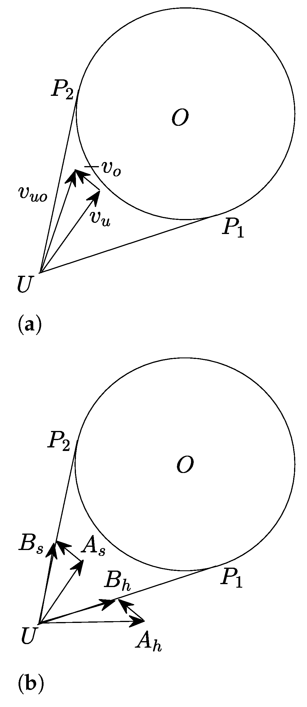
—Relative velocity of the UAV during the hazard stage.
  • v b ( t ) —Relative velocity of the UAV during the intermediate stage.
  • d r —The relative distance between the UAV and the obstacle when the obstacle was initially sensed ( U O distance).
  • r r —The relative distance traveled by the UAV during the intermediate stage from C to A (Figure 6a).
   □
With the availability of range sensors which could measure up to 300 m (e.g.,: LDM301, Sick DME5000-321) we make a reasonable assumption as in Assumption 2.
Assumption 2.
If the radius of the base of the collision cone is R. Then, 10 R d r .
By considering the UAV’s radius along with the secure safety boundary, we introduce a sensible assumption in Assumption 3.
Assumption 3.
For any given collision cone γ + ψ C . Where, A U O = γ , J U O = ψ and C R .
Assumption 4.
Let v b be the maximum relative velocity during the intermediate stage ( v b is the maximum velocity, v b ( t ) could reach). For ease of analysis, we assume that the UAV travels at v b during the intermediate stage.
Let, O C J = ϕ , A U O = γ , J U O = ψ , A O C = θ .
We introduce δ r in Equation (33).
δ r = d r cos ( γ ) ( d r cos ( ψ ) R cos ( ϕ ) ) .
Similar to δ r and r r in the relative scenario, we can also consider δ w and r w in the real scenario. With the aid of Remark 2 and Assumption 3, we can introduce (34) and (35). Where k 1 , k 2 R .
δ r = k 1 δ w
r r = k 2 r w
(36) could be obtained by (35)/(34).
r w δ w = k 1 k 2 r r δ r .
(36) could be rearranged as r w δ w r r δ r . We introduce (37) by applying ϕ = π 2 ( γ + θ ψ ) to (33),
δ r = d r cos ( γ ) ( d r cos ( ψ ) R cos ( π 2 ( γ + θ ψ ) ) ) .
(37) could be simplified as (38).
δ r = d r cos ( γ ) d r cos ( ψ ) + R s i n ( γ + θ ψ ) .
The terms in (38) could be rearranged in the form of (39).
δ r = 2 d r sin ( γ ψ 2 ) sin ( γ + ψ 2 ) + R sin ( θ ) cos ( γ ψ ) + R cos ( θ ) sin ( γ ψ ) .
The term R cos ( θ ) sin ( γ ψ ) of (39) could be expanded as in (40).
δ r = 2 d r sin ( γ ψ 2 ) sin ( γ + ψ 2 ) + R sin ( θ ) c o s ( γ ψ ) + 2 R c o s ( θ ) sin ( γ ψ 2 ) cos ( γ ψ 2 ) .
With the aid of Assumption 2 we apply d r = 10 R to (40).
δ r = 20 R sin ( γ ψ 2 ) sin ( γ + ψ 2 ) + R sin ( θ ) cos ( γ ψ ) + 2 R c o s ( θ ) sin ( γ ψ 2 ) cos ( γ ψ 2 ) .
A simplified version of (41) is presented in (42).
δ r = 2 R sin ( γ ψ 2 ) 10 sin ( γ + ψ 2 ) cos ( θ ) cos ( γ ψ 2 ) + R sin ( θ ) cos ( γ ψ ) .
With the aid of Assumptions 2 and 3 we can state that 10 sin ( γ + ψ 2 ) > 1 and 0 < cos ( θ ) cos ( γ ψ 2 ) < 1 . Therefore, we can confirm that
2 R sin ( γ ψ 2 ) 10 sin ( γ + ψ 2 ) cos ( θ ) cos ( γ ψ 2 ) < 0 . Furthermore, we also can affirm that R sin ( θ ) cos ( γ ψ ) < R sin ( θ ) as 0 < cos ( γ ψ ) < 1 . Thereby, δ r < R sin ( θ ) .
We introduce the definition of r r as in (43).
r r = R θ
Generally radians of θ values are larger or equal to their corresponding sin ( θ ) values. Therefore, r r > δ r . If we consider the real scenario, from (36) we are able to confirm that r w > δ w . The UAV travels in constant v u in the real scenario. As a result, the UAV will travel the δ w distance in a much shorter time compared to the r w distance. As per Remark 2, the time taken to travel δ r will be much lesser than the time taken to travel r r . In essence, the proof made till this point certifies that the UAV’s relative movement through U A edge reaches point A much faster than the other method reaching via point C.
Let B w 1 be the final point of the intermediate stage in the real scenario corresponding to B 1 . According to the Remark 2, the UAV enters B 1 in the relative scenario and B w 1 in the real scenario at the same time. Similarly, let B w 2 be the final point of the intermediate stage in the real scenario which corresponds to B 2 in the relative scenario. The UAV will arrive at B w 1 at first due to the early entrance to the intermediate stage. Thereafter, the UAV will move directly to the goal in a straight line. Point B w 1 always will have a lesser distance to the goal compared to B w 2 (Figure 6b). Therefore, the UAV will be reaching the goal in a much shorter time through B w 1 G . In correspondence, the UAV will relatively move towards the goal through B 1 in a shorter time and reach the goal at G ( t 1 ) if the goal reaching time is t 1 . In conclusion, U A B 1 G ( t 1 ) will be the time-efficient path.
This completes the proof of Theorem 1. We also lay our investigation towards time efficiency comparison between a straight line trajectory (described prior) and non-linear/ piecewise linear paths during the hazard stage in this section. Let a UAV travel to a point on the periphery of the obstacle in a non-straight trajectory in t 1 time by being at a constant speed. The UAV can reach the same point in a straight trajectory in the same constant speed in t 2 time, where t 2 < t 1 . Therefore, if the UAV travels in a constant speed, there will always be a time-efficient linear path to reach a point in the periphery compared to any other non-linear path traveled in the same speed.
It can be confirmed that the PHSO method gives the most time-efficient solution in comparison to PHSI method. Therefore, the PHSO method will be referred as PHS (Purely Heading Solution) through out the rest of the script.

4.4. Comparison of Phs with Pss Method

Theorem 2.
Let T 1 be the completion time of PHS and T 2 be the completion time of PSS. T 1 < T 2 at any given collision cone scenario.
Proof of Theorem 2. 
A collision cone scenario is presented in Figure 7a and the PHS and PSS corrections are shown in Figure 7b. The vector triangle U A s B s represents the correction of PSS and U A h B h represents the correction of PHS. Let, ∠ U A s B s be θ s and ∠ U A h B h be θ h . By applying the law cosines, the magnitude of the relative velocity vector of PSS could be shown as in (44) and the magnitude of the relative velocity vector of PHS could be given by (45). Let, v u 1 be the speed correction of PSS. The UAV travels in v m a x prior to the collision detection.    □
| v s | = | v u 1 | 2 + | v o | 2 2 | v u 1 | | v o | cos ( θ s ) ,
| v h | = | v m a x | 2 + | v o | 2 2 | v m a x | | v o | cos ( θ h ) .
Due to | v h | 2 , | v s | 2 R > 0 , | v u 1 | 2 + | v o | 2 > 2 | v u 1 | | v o | cos ( θ s ) and | v m a x | 2 + | v o | 2 > 2 | v m a x | | v o | cos ( θ h ) . Furthermore, v m a x > v u 1 condition will satisfy v h > v s at all times. It is clear that with v h > v s condition being satisfied, PHS algorithm will make the UAV reach the obstacle’s safety boundary in the minimum time. Similar to the other theorems, we will consider the real scenario to investigate the intermediate and the post-hazard stages. Due to the lead of PHS at the hazard stage and as the speed of PSS during the intermediate stage is lesser than v m a x , the UAV will be made to arrive at the final point of the intermediate stage in a shorter time by the PHS algorithm. As a result, PHS makes the UAV enter the post-hazard stage before PSS. During the post-hazard stage, both PSS and PHS will make the UAV navigate in v m a x . However, due to the early entrance, PHS navigates the UAV towards the goal in much lesser time when compared with PSS.
It is important to note that in some instances UAV’s heading correction of PHS will make the relative vector coincide with U P 1 edge. In these situations, moving towards P 1 becomes more time-efficient than moving towards P 2 . Therefore, the theorem still becomes valid. This completes the proof of Theorem 2.

4.5. Comparison of Phs with Speed and Heading Hybrid Method

Hitherto, we have discussed PHS and PSS approaches in detail. Similar to PHS and PSS, a speed variation along with a heading variation becomes feasible when avoiding collisions. Two example hybrid approaches are presented in Figure 8. Let v m a x and θ u be the speed and the heading of the UAV prior to the collision. We confirm that v u < v m a x . The angle θ 3 is the angle opposite v u o 3 and θ 4 is opposite to v u o 4 . It is important to compare the time-efficiency merits of the hybrid method with that of PHS at the outset.
Proposition 1.
There are n (where n R ) hybrid methods to avoid a collision, given a collision cone scenario. Let T i be the completion time of a hybrid method, where i 1 n . Let T h be the completion time of the PHS of the same collision scenario. Then, T i > T h .
Proof of Proposition 1. 
The resultant velocities are introduced as in (46) and (47).
| v o u 3 | = ( | v u | ) 2 + | v o | 2 2 | v u | | v o | cos ( θ 3 ) ,
| v o u 4 | = ( | v u | ) 2 + | v o | 2 2 | v u | | v o | cos ( θ 4 ) .
From Theorem 1 we can establish that v u o 4 will make the UAV reach the obstacle’s safety boundary at the earliest. If  v u is increased to v m a x by maintaining the heading, we can assure that the resultant relative velocity will be greater than v u o 4 . This will eventually be the PHS solution. Any hybrid correction that happens inside the collision cone could be stated in the form of (46). The resultant relative velocity could be given by (47) if the relative velocity vector of any hybrid correction coincides with the edge of the collision cone. Therefore, the PHS method will be more time-efficient than any of the hybrid solutions. According to Theorem 1 and Theorem 2, the method that makes the UAV reach the safety margin of the obstacle at first will surely reach the goal ahead of the other methods.    □
This completes the proof of Proposition 1. It is clear that PHS becomes the most time-efficient method to avoid a collision in a single obstacle collision cone scenario.

5. Multiple Collision Handling

A multiple collision situation is where a UAV senses multiple obstacles in a given time instance, which would lead to future collisions. In this section, we introduce an algorithm for a general multiple collision situation initially. Thereafter, an enhanced version of the introduced algorithm will be presented to handle complex multiple obstacle scenarios.

5.1. Typical Multiple Collision Handling

A typical multiple collision example is shown in Figure 9a. As per the conclusions made in the previous section, the time-efficiency of the PHS approach out performs all the remaining avoidance methods that could be used in collision cone scenarios. Navigating on full speed on a straight line during the hazard stage stands the crux of the PHS approach. A multiple collision scenario is a combination of several single collision cones. As per the merits discussed, we consider the application of PHS in multiple collision situations. The aim will be to navigate the UAV in full speed on a straight line.
Figure 9a depicts a multiple collision scenario with two obstacles. Let R O 1 be the radius of obstacle O 1 and R O 2 be the radius of obstacle O 2 . As the initial step, collision cones will be constructed with all the available obstacles. Due to the multiple obstacle nature, unlike in the single obstacle problem, both clockwise and anti-clockwise heading corrections should be considered in each collision cone. As an example, v u o 1 could be made to coincide with U P 1 or U P 2 . As some of the relative vectors are much closer to the bottom edge of the collision cone and some others are closer to the top edge of the collision cone, calculating the heading θ c t in both directions becomes crucial.
Let the number of sensed obstacles be n. Where, n N . With the aid of the PHS algorithm we calculate the clockwise heading correction angle Ω i for each collision cone { i = 1 , , n } . Similarly, we calculate the anti-clockwise heading correction angle η i for each collision cone. From all the Ω i values, we select the maximum as in (48).
Ω m a x = m a x { Ω 1 , , Ω n } .
Similarly, we repeat the selection for η i as in (49).
η m a x = m a x { η 1 , , η n } .
Finally, the minimum value from Ω m a x and η m a x is selected as in (50).
θ c t = m i n { η m a x , Ω m a x } .
Equations (48)–(50) should be calculated at every sample time. The calculated θ c t values from (50) are used throughout the hazard stage. At the last part of the hazard stage the UAV arrives at the safety boundary of one obstacle from the lot. Therefore, the intermediate stage and the post-hazard stage will be similar to the single obstacle scenario. If the UAV encounters another obstacle during the intermediate stage, the collision is handled with a new collision cone.

5.2. Complex Multiple Collision Handling

Figure 9b illustrates a different collision scenario not described before. The UAV in the image has encountered four unattached obstacles. As per the collision cones, UAV has a risk of colliding with O 2 and O 3 initially. If the UAV makes an anticlockwise heading correction, the risk of colliding with O 1 increases. On the other hand, a clockwise correction escalates the risk of impact with O 4 . Therefore, we enhance the PHS method made for multiple collisions introduced in Section 5.1. Algorithm 4 introduces the enhancement. Let there be n number of obstacles sensed. Out of the obstacles, the UAV has a risk of immediately colliding with m number of obstacles. Where, m < n . χ i and Υ i (where, { i = 1 , , n } ) refers to χ and Υ angles of the ith obstacle (Definition 2).
With the introduction of Algorithm 2, we can confirm that there is always a feasible way of avoiding a collision in a time-efficient manner irrespective of the complexity of the collision.
Algorithm 2 Calculation of θ c t in a complex situation.
    Input: η 1 η n , Ω 1 Ω n
    Output: θ c ( t )
  • while 1 do
  •      k m
  •      η m a x m a x { η 1 , , η m } ;
  •      Ω m a x m a x { Ω 1 , , Ω m } ;
  •      θ c t m i n { η m a x , Ω m a x } ;
  •     if  χ k + 1 > Υ k + 1  then
  •        b r e a k ;
  •     end if
  •      m m + 1 ;
  • end while

6. Results

6.1. Simulation Results

The section assesses the performance of the PSS and PHS algorithms in different collision scenarios. The simulations were conducted in a Matlab based testing platform.

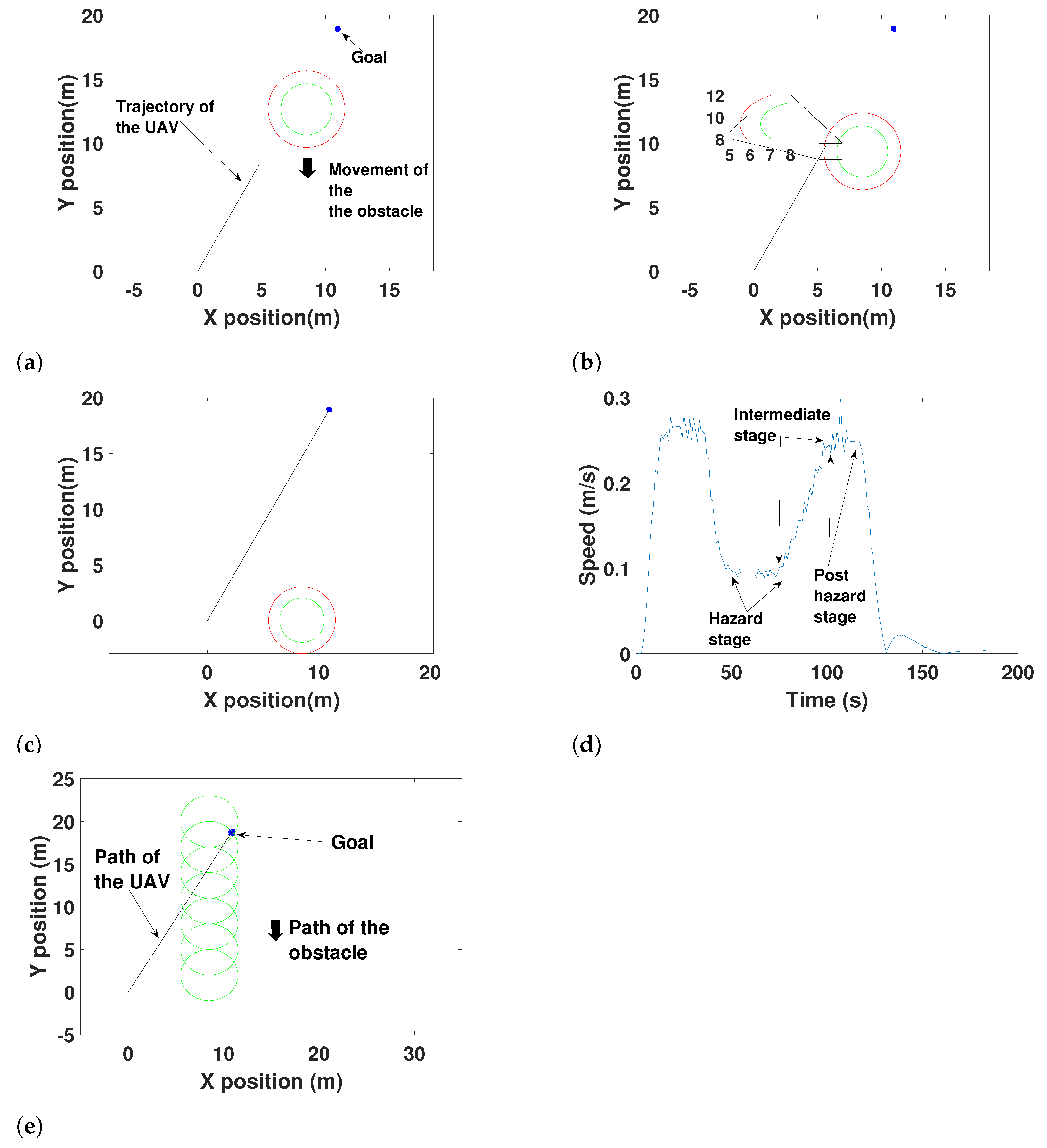
6.1.1. Simulations Related to Pss Algorithm

The UAV in Figure 10 has traveled to a goal located at (300, 300) from the initial starting location. However, it has been obstructed by a dynamic obstacle as shown in Figure 10a. The UAV has maneuvered at a close proximity to the obstacle’s surface during the intermediate stage with the aid of (11). As per the velocity profile shown in Figure 10d, the velocity has been around 1.4 ms 1 throughout the hazard stage as a result of (5). The UAV has passed the intermediate stage swiftly with the aid of (11) which was introduced in Section 3.1.2.

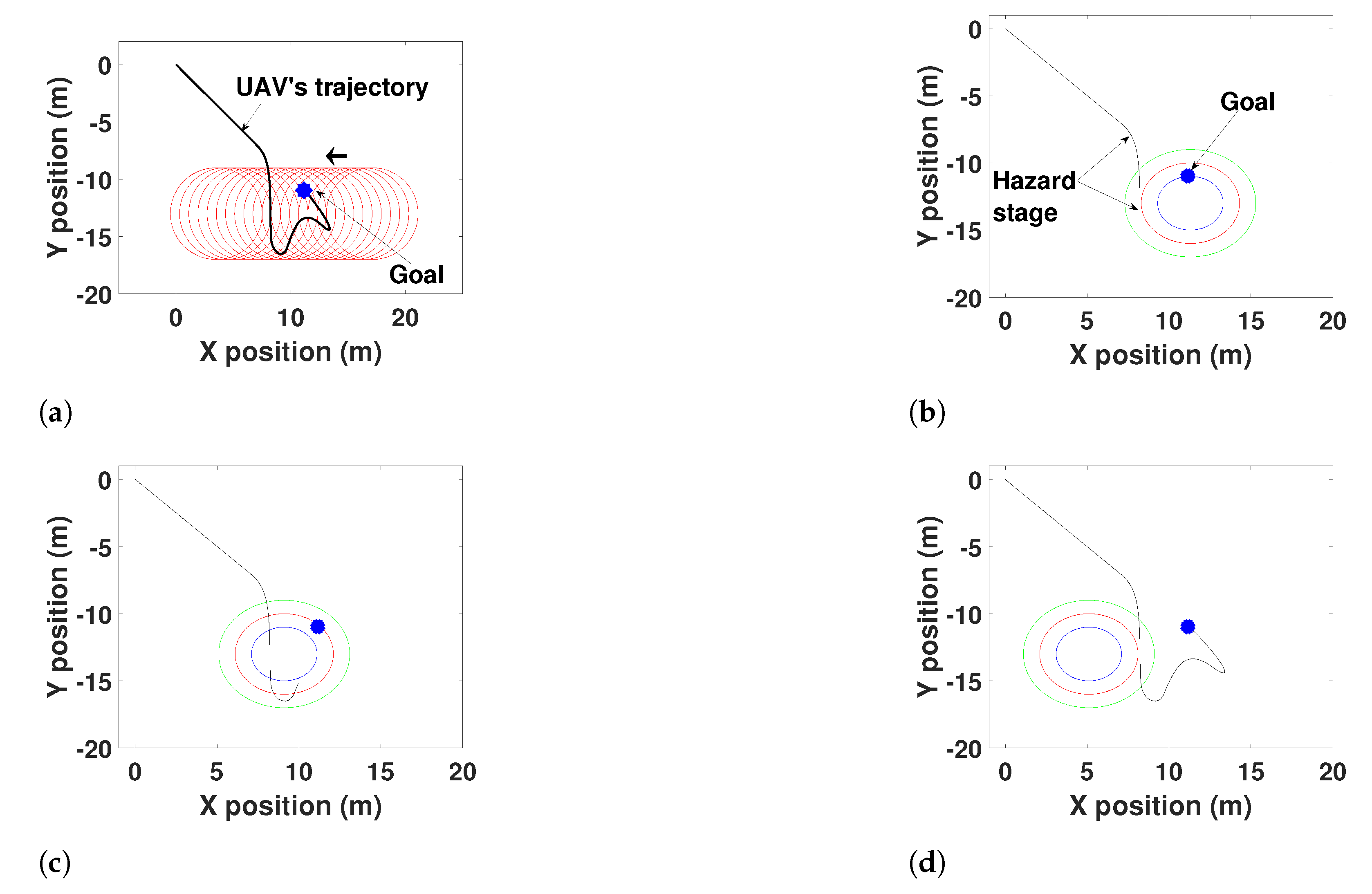
6.1.2. Simulations Related to Phs Algorithm

A typical PHS scenario is presented in Figure 11. The UAV has navigated in a speed of 5 ms 1 . As mentioned in Section 4.2.2, an additional safety boundary has been introduced for the intermediate stage. Figure 11a shows the full trajectories of the UAV and obstacle. The operation of the sliding mode controller is quite observable in the hazard stage depicted in Figure 11b. The last point of the hazard stage (which is zoomed in and presented) is clearly positioned in between the obstacle’s surface and the exterior safety boundary. Algorithm 1 hasn’t allowed the UAV to collide with the obstacle or to reach out of the exterior safety boundary. Figure 11c delineates the post-hazard stage with a straight trajectory directly towards the goal.

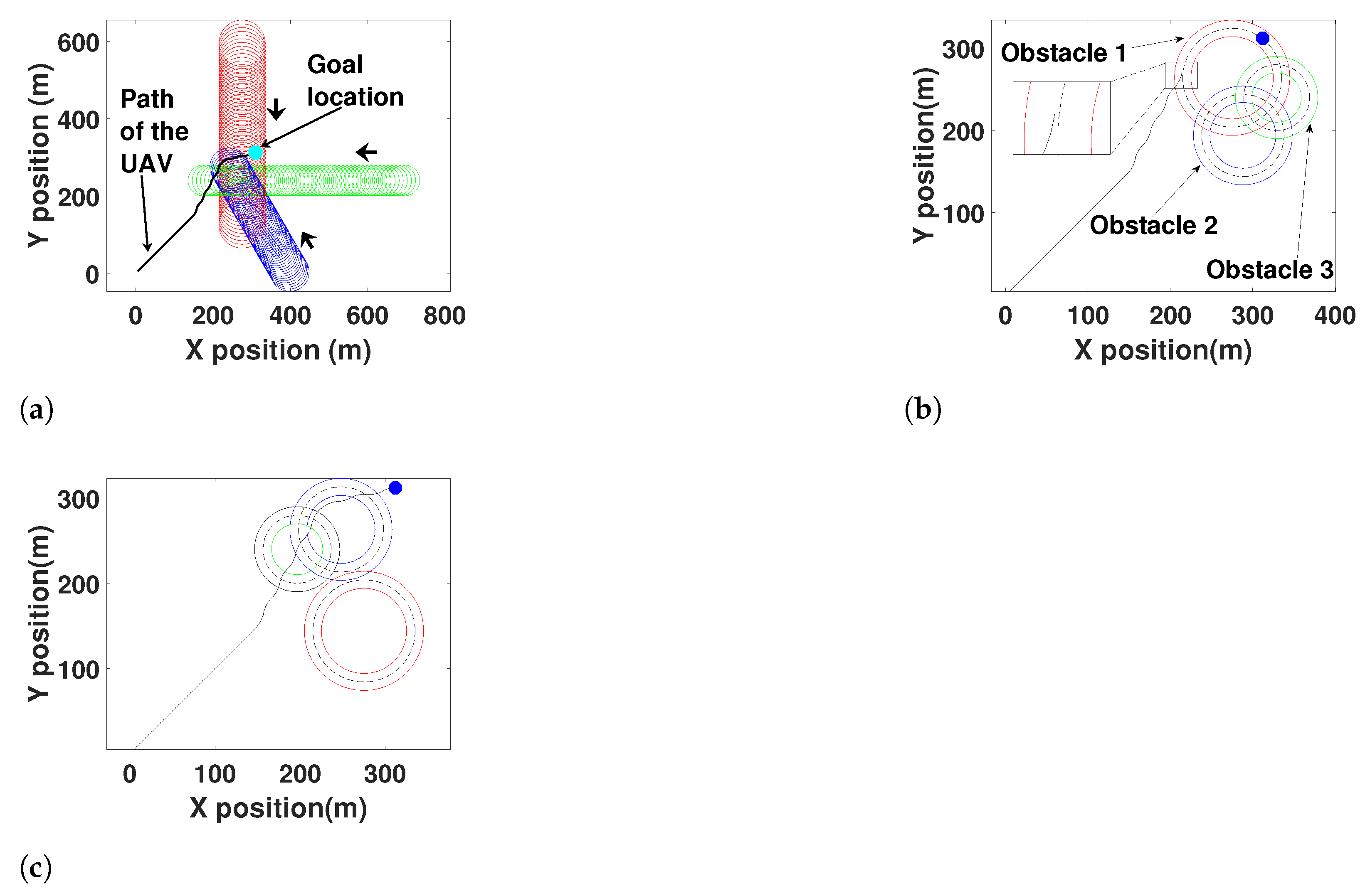
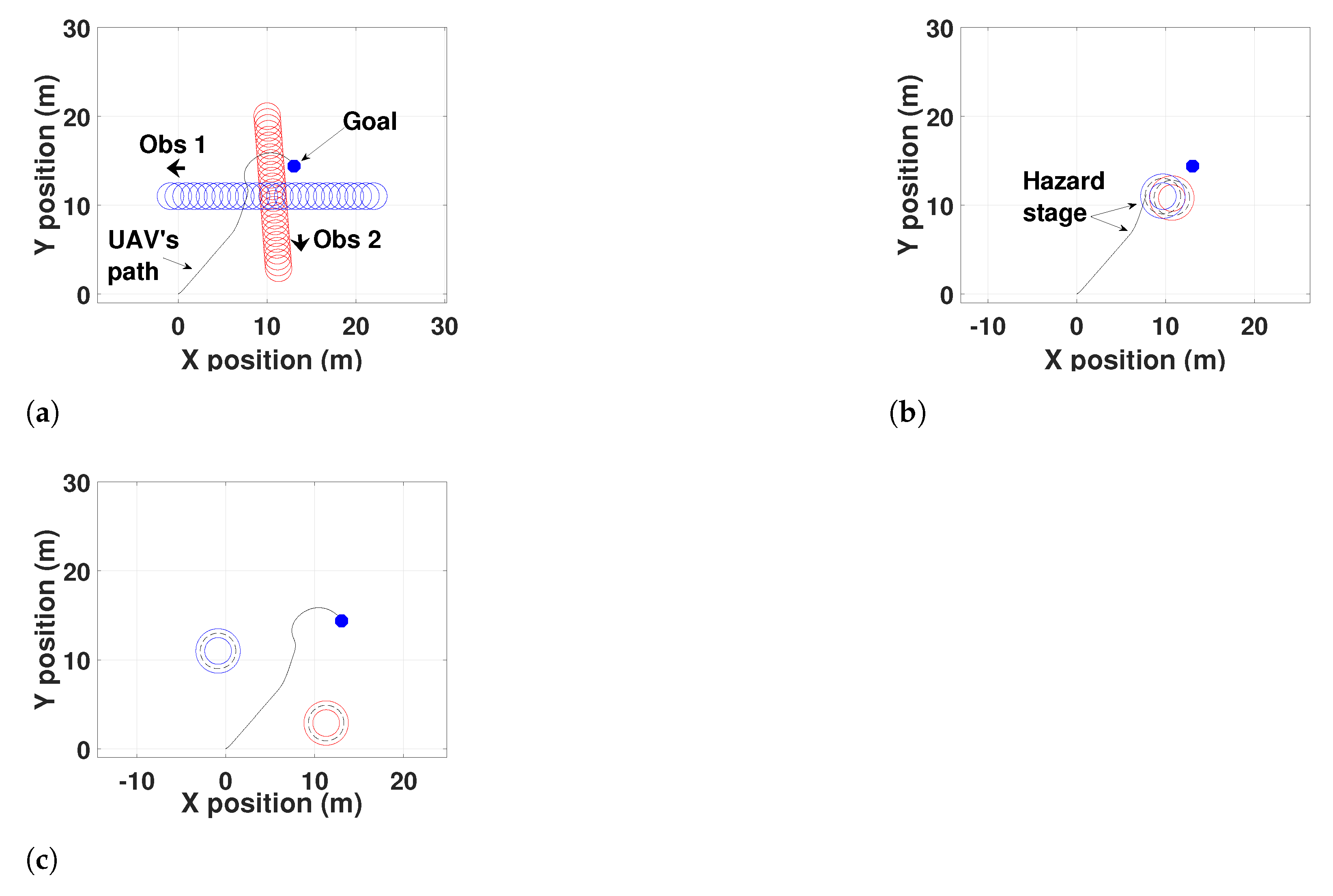
6.1.3. Multiple Collision Avoidance Handing

Figure 12 shows a collision avoidance situation with three obstacles with different radii. The UAV has been navigated to the safety margin of obstacle 1 by Equation (50) as presented in Figure 12b. It is important to note that Equation (50) hasn’t maneuvered the UAV to the safety boundaries of obstacle 2 and obstacle 3 as a result of potential collisions. The last point of the hazard stage has been zoomed in and presented. In Figure 12, the UAV has avoided the obstacles satisfying the equations introduced in Section 5.1 and have successfully maneuvered to the goal location.

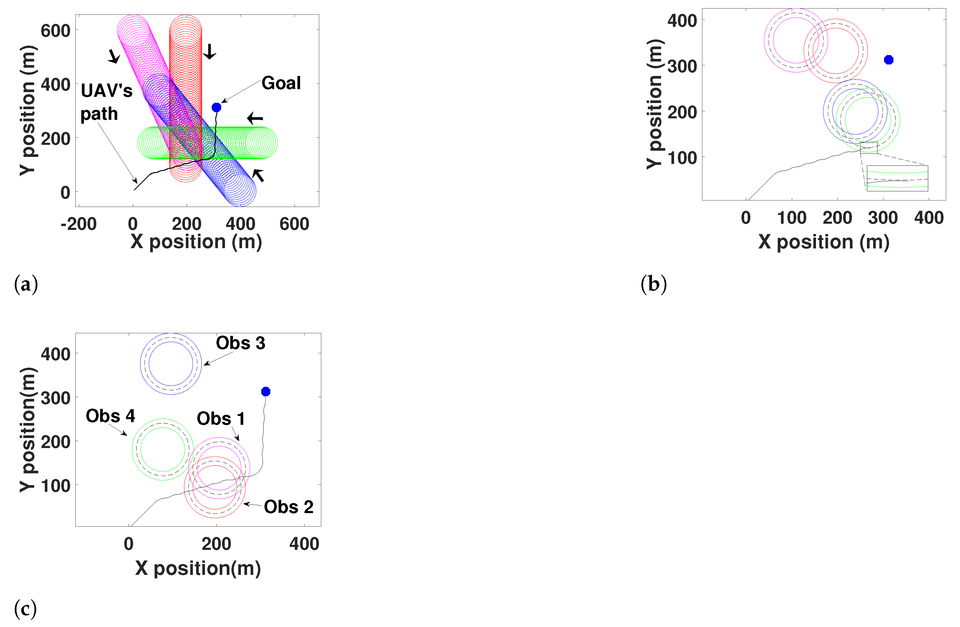
6.1.4. Complex Collision Avoidance

A complex multiple collision avoidance situation is illustrated in Figure 13. The trajectory profiles are presented in Figure 13a. The UAV, which traveled in a 5 ms 1 speed, has initially encountered obstacle 2 and obstacle 3 around (70,70) as potential threats while traveling towards the goal location. The UAV will not be able to make an anti-clockwise heading correction to move towards the safety margin of obstacle 2, as it would enter the collision cone of obstacle 1. Similarly, it does not have the ability to reach the safety margin of obstacle 3, as it would enter the collision cone of obstacle 4. Therefore, with the aid of Algorithm 3 introduced in Section 5.2, the UAV has navigated to the safety margin of obstacle 4 as shown in Figure 13b. After avoiding the collision, the UAV has successfully reached the goal according to Figure 13c.

6.1.5. A Simulation to Justify Theorems 1 and 2

The purpose of this simulation is to justify Theorems 1 and 2. In order to test the validity of Theorem 1, we make the UAV travel through the points labeled in Figure 6a. In other words, U E A , U D A , U C A , U F A , U H A , U I A segments separately and to reach the goal according to PHSI algorithm. Thereafter, the UAV is sent through the U A edge to reach the goal as stated in the PHS algorithm. In order to examine Theorem 2, the collision situation is once more handled using the PSS method. More importantly, the completion time of each and every method is recorded for comparison. Figure 14 presents the completion time results of each method, which justifies Theorems 1 and 2.

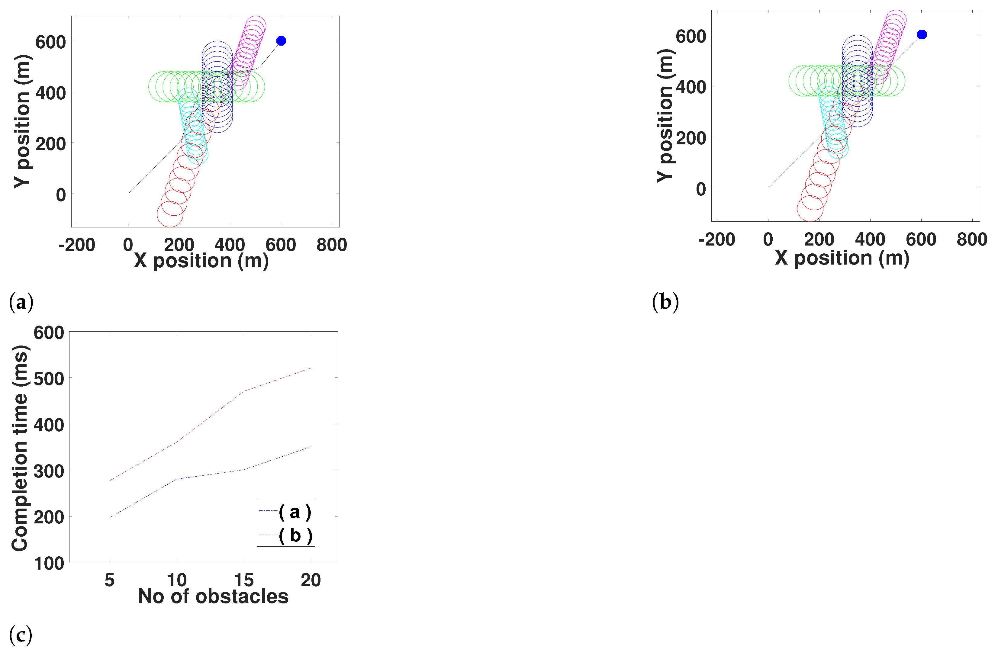
6.1.6. Comparison with Tscc (Time Scaled Collision Cone) Method

Authors in [17] use nonlinear time scaling [18] to avoid collisions by acceleration or retardation. It is the sole approach or benchmark method that proposes a time-efficient collision avoidance paradigm for collision cones as mentioned in the literature review. We have compared our PHS approach with the TSCC method proposed in [17] in Figure 15. Both the algorithms were applied in the same environment, and the task completion time has been recorded. Figure 15a,b illustrates the behavior of the algorithms in a five obstacle environment. To normalize both scenarios and to present in real-time, we have set the max speed of the UAV as 5 ms 1 . A completion time of 196.63 ms was recorded by the PHS algorithm and the TSCC has recorded 276 ms to complete the five obstacle avoidance task. By having the same goal position as in Figure 15a,b, we have increased the number of obstacles and recorded the completion time in Figure 15c in order to draw a proper conclusion. In Figure 15c, the number of obstacles has been increased to 10, 15 and 20 (due to the high clutteredness, these situations will not be illustrated). It is more than clear that the PHS method’s time-efficiency outperforms that of TSCC method.
It is fair to say, that the simulation results presented in this section solidly ratify the theories discussed in Section 3, Section 4 and Section 5.

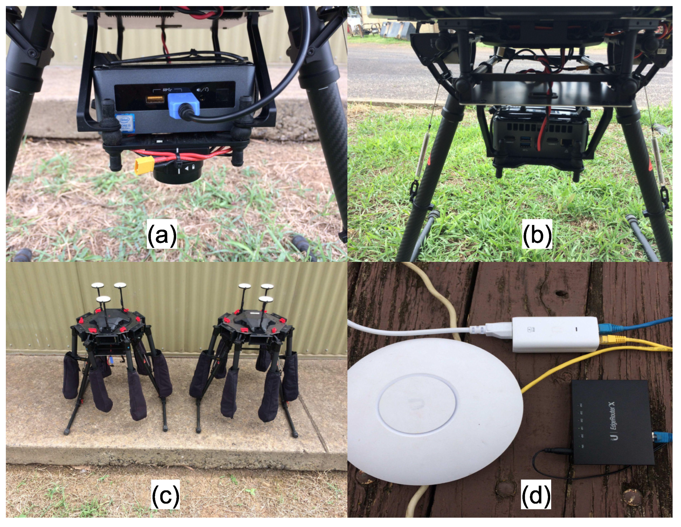
6.2. Experimental Results

A set of physical experiments were conducted to ensure the practicality of the PHS method. The practical set-up and equipment used are shown in Figure 16. A Matrice 600 PRO hexacopter is used as the UAV. An Intel NUC mini PC is used to automate the hexacopter. The mini PC is connected to the hexacopter via a USB cable and powered by the battery power of the hexacopter. Since obstacles are UAVs in reality, the available other hexacopters in the laboratory can be used as obstacles for the experiments with a similar automation set-up. However, as the wind condition is not addressed in this research fictitious obstacles are used as a safety measure. In addition, we have built up a wireless local area network (WLAN) with the aid of an Ubiquiti Edge router, an Ubiquiti access point and a laptop computer. All computers are connected to the network so that data such as the location of a hexacopter could be shared among the computers. Ubuntu operating systems are installed in all the computers. In addition, we have installed DJI SDK 3.6 to access the flight controller (A3 pro) of the hexacopter. The algorithm is coded in C++. The experiments were conducted in an open field in Menangle, New South Wales, Australia.
With the aid of the above set-up, we have conducted single obstacle and multiple obstacle related experiments of the PHS algorithm. The τ value of (16) is replaced by a heading angle of 1 rad. As a result, the UAV’s controller will be switching between −1 rad, 0 rad and +1 rad. The starting location of the UAV will be considered the origin, and all the graph co-ordinates in this section are with respect to the origin. With a reasonable safety boundary, the radius of a hexacopter could be stated as 1.5 m.
Figure 17 presents the single obstacle experiment based on speed. The hexacopter has traveled in a 0.26 ms 1 speed in a heading direction of π / 3 rad. The obstacle has traveled in a direction of π / 2 rad and in a speed of 0.15 ms 1 . Figure 17a shows the hazard stage. A sample of the intermediate stage is presented in Figure 17b and it is more than clear that the hexacopter hasn’t been collided with the obstacle. Figure 17c presents the goal reaching moment. The complete speed profile is shown in Figure 17d. Some spikes in the speed profile can be observed. This is primarily due to external resistances. Figure 17e has shown the complete trajectory of the obstacle and the hexacopter.
The full trajectory profiles of the UAV and the obstacle is shown in Figure 18a. As the controller is switching between −1 rad and 1 rad, a trajectory oscillation (switching due to the sliding mode controller) is not visible as in the simulations during the hazard stage (Figure 18b). The UAV has successfully reached the safety boundary of the obstacle. Figure 18c shows a sample of the intermediate stage. Even though Algorithm 1 has navigated the UAV successfully, the travel trajectory during the intermediate stage hasn’t been smooth when compared to the simulations. The main reason behind this difference is the dynamics of the UAV (hexacopter) and the external influences such as wind. Figure 18d presents the goal reaching moment of the UAV. It is clear that the dynamics haven’t allowed the UAV to make a swift heading change to reach the goal. Hence, it has made a 3.14 rad sluggish heading change to reach the goal.
Figure 19 shows a potential multiple collision situation with two obstacles. Figure 19b depicts the successful completion of hazard stage by the use of (50). In Figure 19c, the UAV has reached the goal successfully. However, due to the dynamics and external resistances, it has reached the goal with moderate heading changes. Hence, it hasn’t been able to navigate directly towards the goal.
In summary, the main differences between the experimental results and the simulation results are the dynamics of the UAV and external resistances such as the wind. However, the experimental results firmly validate the PHS algorithm.

7. Conclusions

A UAV could avoid a potential collision with dynamic obstacles either by changing the speed or changing its heading or by changing both speed and heading concurrently. This paper has thoroughly investigated all three possibilities and has shown that the heading based method is time-efficient than the other two. The paper has proposed PHS (Purely Heading Solution) method and has confirmed the time-efficiency with rigorous mathematical proofs. Initially, the PHS method was first implemented for a single obstacle and thereafter enhanced and implemented to avoid multiple and complex collision scenarios. Furthermore, the time-efficiency of PHS was shown to be better when the results were compared with other work in literature. The validity of the proposed method was demonstrated both in simulation and real flight experiments.
As future work, the proposed PHS method will be enhanced to perform in 3D environments. Furthermore, the impact of the wind resistance will be addressed with the aid of an additional controller.

Author Contributions

Conceptualization, M.G. and J.K.; methodology, M.G.; software, M.G.; validation, M.G. and J.K.; formal analysis, M.G.; investigation, M.G.; resources, J.K.; data curation, M.G.; writing—original draft preparation, M.G.; writing—review and editing, M.G.; visualization, M.G.; supervision, J.K.; project administration, J.K.; funding acquisition, J.K. All authors have read and agreed to the published version of the manuscript.

Funding

This research received no external funding.

Institutional Review Board Statement

Not applicable.

Informed Consent Statement

Not applicable.

Data Availability Statement

Not applicable.

Conflicts of Interest

The authors declare no conflict of interest.

References

  1. Kavraki, L.E.; Svestka, P.; Latombe, J.C.; Overmars, M.H. Probabilistic roadmaps for path planning in high-dimensional configuration spaces. IEEE Trans. Robot. Autom. 1996, 12, 566–580. [Google Scholar] [CrossRef] [Green Version]
  2. Hart, P.E.; Nilsson, N.J.; Raphael, B. A formal basis for the heuristic determination of minimum cost paths. IEEE Trans. Syst. Sci. Cybern. 1968, 4, 100–107. [Google Scholar] [CrossRef]
  3. Stentz, A. Optimal and efficient path planning for partially known environments. In Intelligent Unmanned Ground Vehicles; Springer: Berlin/Heidelberg, Germany, 1997; pp. 203–220. [Google Scholar]
  4. LaValle, S.M.; Cheng, P. Resolution complete rapidly-exploring random trees. In Proceedings of the 2002 IEEE International Conference on Robotics and Automation (Cat. No. 02CH37292), Washington, DC, USA, 11–15 May 2002; Volume 1, pp. 267–272. [Google Scholar]
  5. Borenstein, J.; Koren, Y. The vector field histogram-fast obstacle avoidance for mobile robots. IEEE Trans. Robot. Autom. 1991, 7, 278–288. [Google Scholar] [CrossRef] [Green Version]
  6. Fox, D.; Burgard, W.; Thrun, S. The dynamic window approach to collision avoidance. IEEE Robot. Autom. Mag. 1997, 4, 23–33. [Google Scholar] [CrossRef] [Green Version]
  7. Khatib, O. Real-time obstacle avoidance for manipulators and mobile robots. In Autonomous Robot Vehicles; Springer: Berlin/Heidelberg, Germany, 1986; pp. 396–404. [Google Scholar]
  8. Chakravarthy, A.; Ghose, D. Obstacle avoidance in a dynamic environment: A collision cone approach. IEEE Trans. Syst. Man Cybern. Part A Syst. Hum. 1998, 28, 562–574. [Google Scholar] [CrossRef] [Green Version]
  9. Fiorini, P.; Shiller, Z. Motion planning in dynamic environments using velocity obstacles. Int. J. Robot. Res. 1998, 17, 760–772. [Google Scholar] [CrossRef]
  10. Large, F.; Sckhavat, S.; Shiller, Z.; Laugier, C. Using non-linear velocity obstacles to plan motions in a dynamic environment. In Proceedings of the 7th International Conference on Control, Automation, Robotics and Vision, (ICARCV 2002), Singapore, 2–5 December 2002; IEEE: Piscataway, NJ, USA, 2002; Volume 2, pp. 734–739. [Google Scholar]
  11. Fulgenzi, C.; Spalanzani, A.; Laugier, C. Dynamic obstacle avoidance in uncertain environment combining PVOs and occupancy grid. In Proceedings of the 2007 IEEE International Conference on Robotics and Automation, Rome, Italy, 10–14 April 2007; IEEE: Piscataway, NJ, USA, 2007; pp. 1610–1616. [Google Scholar]
  12. Kluge, B.; Prassler, E. Reflective navigation: Individual behaviors and group behaviors. In Proceedings of the IEEE International Conference on Robotics and Automation, 2004. Proceedings. ICRA’04. 2004, New Orleans, LA, USA, 26 April–1 May 2004; IEEE: Piscataway, NJ, USA, 2004; Volume 4, pp. 4172–4177. [Google Scholar]
  13. Van den Berg, J.; Lin, M.; Manocha, D. Reciprocal velocity obstacles for real-time multi-agent navigation. In Proceedings of the 2008 IEEE International Conference on Robotics and Automation, Pasadena, CA, USA, 19–23 May 2008; IEEE: Piscataway, NJ, USA, 2008; pp. 1928–1935. [Google Scholar]
  14. Snape, J.; Van Den Berg, J.; Guy, S.J.; Manocha, D. Independent navigation of multiple mobile robots with hybrid reciprocal velocity obstacles. In Proceedings of the 2009 IEEE/RSJ International Conference on Intelligent Robots and Systems, St. Louis, MO, USA, 10–15 October 2009; IEEE: Piscataway, NJ, USA, 2009; pp. 5917–5922. [Google Scholar]
  15. Guy, S.J.; Chhugani, J.; Kim, C.; Satish, N.; Lin, M.; Manocha, D.; Dubey, P. Clearpath: Highly parallel collision avoidance for multi-agent simulation. In Proceedings of the 2009 ACM SIGGRAPH/Eurographics Symposium on Computer Animation, New Orleans, LA, USA, 1–2 August 2009; pp. 177–187. [Google Scholar]
  16. Singh, A.K.; Krishna, K.M. Reactive collision avoidance for multiple robots by non linear time scaling. In Proceedings of the 52nd IEEE Conference on Decision and Control, Florence, Italy, 10–13 December 2013; IEEE: Piscataway, NJ, USA, 2013; pp. 952–958. [Google Scholar]
  17. Gopalakrishnan, B.; Singh, A.K.; Krishna, K.M. Time scaled collision cone based trajectory optimization approach for reactive planning in dynamic environments. In Proceedings of the 2014 IEEE/RSJ International Conference on Intelligent Robots and Systems, Chicago, IL, USA, 14–18 September 2014; IEEE: Piscataway, NJ, USA, 2014; pp. 4169–4176. [Google Scholar]
  18. Gnanasekera, M.; Katupitiya, J. A Time Optimal Reactive Collision Avoidance Method for UAVs Based on a Modified Collision Cone Approach. In Proceedings of the 2020 IEEE/RSJ International Conference on Intelligent Robots and Systems, Las Vegas, NV, USA, 25–29 October 2020; IEEE: Piscataway, NJ, USA, 2020; pp. 5685–5692. [Google Scholar]
Figure 1. The collision cone is drawn with respect to the obstacle’s velocity. The UAV is traveling in v u and the obstacle is traveling in v o . The UAV has a radius of R u and the obstacle has a radius of R o . The UAV is drawn as a point and the obstacle is drawn with a radius of R u + R o .
Drones 06 00106 g001
Figure 2. The figure shows a typical potential collision situation between a UAV and an obstacle. The two sub-figures show the real scenario (the actual situation) and the relative (with respect to the obstacle) scenario. (a) The actual travel path of the UAV is U G and the obstacle’s trajectory intersects the path at C. (b) Shows the relative travel path. Point W is the replica of D in the relative scenario. When the UAV actually moves from U to G, relatively it travels in the U B direction.
Drones 06 00106 g002
Figure 3. The subfigures show the corrections required during the hazard stage and the intermediate stage. The speed correction during the hazard stage and the intermediate stages. (a) The relative velocity vector triangles after the speed correction is shown. v u o is the is the relative velocity vector after the speed is corrected. v u o coincides with U T 2 line segment. (b) The intermediate stage when considering the UAV’s relative motion. X O is parallel to the X-axis/abscissa. T 2 is the entrance point of the intermediate stage. W is the final point of the intermediate stage.
Drones 06 00106 g003aDrones 06 00106 g003b
Figure 4. The collision scenario and the possible heading corrections. (a) A potential collision with UAV U and obstacle O. In the relative scenario, the UAV will meet the goal at G in the presence of no collision. (b) Different directions that the v u o vector could be directed at. Vectors U C and U B will navigate the UAV inside the collision cone until the safety boundary of the obstacle. On the other hand, vectors U D , U A , U E , U F will immediately move the UAV out of the collision cone.
Drones 06 00106 g004
Figure 5. The relative velocity vector triangles needed for the angle calculations are shown in this figure. Heading correction during the hazard stage. U H 1 N 1   is the relative vector triangle prior to the heading correction. U H 2 N 2   is the relative vector triangle after the heading correction.
Drones 06 00106 g005
Figure 6. The figures explains the P H S I method. Especially the hazard stage and the intermediate stage. (a) The points on the obstacle’s periphery (safety boundary) which are inside the collision cone are labeled as A, C, D, E, F, H, I. (b) Post-hazard stages of the two cases. B w 1 is the final point of the intermediate stage of the case coming through A. B w 2 is the final point of the case coming through C.
Drones 06 00106 g006
Figure 7. The figures represent a collision scenario and the corresponding P H S and P S S corrections in form of relative velocity vector triangles: (a) Presents the scenario prior to the correction. (b) Shows P H S and P S S corrections.
Drones 06 00106 g007
Figure 8. The two relative vectors represent the hazard stages of two hybrid methods. Where, v u < v u .
Drones 06 00106 g008
Figure 9. Multiple collision avoidance: (a) A typical collision situation with two obstacles. Since, v u o 1 and v u o 2 are inside the collision cones the UAV will be colliding with both O 1 and O 2 obstacles. (b) presents a complex multiple obstacle scenario. Where, the UAV has a risk colliding with O 2 and O 3 initially. With a clockwise correction, the UAV has a risk of colliding with O 1 . With an anti-clockwise correction, the UAV has a risk of colliding with O 4 .
Drones 06 00106 g009
Figure 10. Simulation conducted on the purely speed scenario: (a) Shows the hazard stage. Figures (b) illustrates the intermediate stage. (c) Shows the post hazard stage. (d) Shows the speed profile of UAV.
Drones 06 00106 g010
Figure 11. Simulation conducted on the purely heading scenario. The obstacle has traveled at a speed of 4.9 ms 1 and moved at a direction of 3 π / 2 rad from the X-axis. The UAV has traveled towards a goal located at (250,250): (a) Shows the full trajectory of the UAV and the obstacle. (b) Presents the hazard stage. The point at which the UAV enters the safety margin of the obstacle has been zoomed in and presented. (c) Depicts the goal reaching moment (post-hazard stage).
Drones 06 00106 g011
Figure 12. Multiple collision avoidance with three obstacles. Obstacle 1 moves in a speed of 4.8 ms 1 in a direction of 1.5708 rad, obstacle 2 moves in a direction of 2.0944 rad at a speed of 3.2 ms 1 and obstacle 3 moves at an angle −3.1416 rad in a speed 4.3 ms 1 : (a) Shows the full trajectory profiles. (b) Presents the hazard stage. (c) Shows the successful completion of the task during the post-hazard stage.
Drones 06 00106 g012
Figure 13. Complex multiple collision scenario. Obstacle 1 has traveled at a speed of 4.4 ms 1 in a heading of 1.15 rad, obstacle 2 has moved with a heading of 1.57 rad with a speed of 4.4 ms 1 , obstacle 3 has traveled in a heading direction of 2.25 rad with a speed of 4.2 ms 1 and obstacle 4 has traveled at a speed of 3.5 ms 1 in a direction of −3.14 rad.: (a) Shows the full trajectory profiles. (b) Shows the hazard stage and the last point of the hazard stage is zoomed. (c) Presents post-hazard stage.
Drones 06 00106 g013
Figure 14. Shows the completion times taken by different methods. Labels I, H, F, C, D, E represents the path through each point.
Drones 06 00106 g014
Figure 15. Comparison between PHS and TSCC: (a) Shows the trajectory profiles of the PHS method and five different obstacles. (b) Shows the trajectory profiles of the same five obstacles and the TSCC method. (c) Shows the time taken by PHS and TSCC to complete a task when the number of obstacles are increased.
Drones 06 00106 g015
Figure 16. Equipment used for the experiments: (a) Shows the NUC mini PC connected to the flight controller via a USB cable. (b) Shows the NUC mini PC and the power connection which is provided from the hexacopter batteries. (c) Hexacopters available in the laboratory. The radius of a hexacopter with a reasonable safety boundary is around 1.5 m. (d) Shows the Edge router and the access point.
Drones 06 00106 g016
Figure 17. Speed experiment: (a) shows the hazard stage. (b) illustrates a samples of the intermediate stage. (c) shows the post hazard stage. (d) shows the speed profile of UAV. (e) Complete trajectories of the UAV and the obstacle.
Drones 06 00106 g017
Figure 18. First experiment conducted on the purely heading scenario with a single obstacle. The hexacopter has navigated in a speed of 0.3 ms 1 towards a goal located at (10.69,−10.69) and has encountered as potential threat by an obstacle traveling at a speed of 0.1 ms 1 in a direction of 3.14 rad.: (a) shows the full trajectory of the hexacopter and the obstacle. (b) presents the hazard stage. (c) shows a sample from the intermediate stage. (d) depicts the goal reaching moment (post-hazard stage).
Drones 06 00106 g018
Figure 19. Experiment on avoiding two obstacles. The hexacaopter has traveled at a speed of 0.31 ms 1 towards a goal located around (13, 14). Obstacle 1 has moved in a speed of 0.165 ms 1 in direction of a −3.14 rad, and obstacle 2 has moved in a speed of 0.22 ms 1 in a heading angle of −1.4960 rad: (a) shows the full trajectories of the hexacopter and the obstacles. (b) shows the hazard stage. (c) presents the goal reaching moment during the post-hazard stage.
Drones 06 00106 g019
Publisher’s Note: MDPI stays neutral with regard to jurisdictional claims in published maps and institutional affiliations.

