New Supplementary Photography Methods after the Anomalous of Ground Control Points in UAV Structure-from-Motion Photogrammetry

Abstract

Recently, multirotor UAVs have been widely used in high-precision terrain mapping, cadastral surveys and other fields due to their low cost, flexibility, and high efficiency. Indirect georeferencing of ground control points (GCPs) is often required to obtain highly accurate topographic products such as orthoimages and digital surface models. However, in practical projects, GCPs are susceptible to anomalies caused by external factors (GCPs covered by foreign objects such as crops and cars, vandalism, etc.), resulting in a reduced availability of UAV images. The errors associated with the loss of GCPs are apparent. The widely used solution of using natural feature points as ground control points often fails to meet the high accuracy requirements. For the problem of control point anomalies, this paper innovatively presents two new methods of completing data fusion by supplementing photos via UAV at a later stage. In this study, 72 sets of experiments were set up, including three control experiments for analysis. Two parameters were used for accuracy assessment: Root Mean Square Error (RMSE) and Multiscale Model to Model Cloud Comparison (M3C2). The study shows that the two new methods can meet the reference accuracy requirements in horizontal direction and elevation direction (RMSE_X = 70.40 mm, RMSE_Y = 53.90 mm, RMSE_Z = 87.70 mm). In contrast, the natural feature points as ground control points showed poor accuracy, with RMSE_X = 94.80 mm, RMSE_Y = 68.80 mm, and RMSE_Z = 104.40 mm for the checkpoints. This research considers and solves the problems of anomalous GCPs in the photogrammetry project from a unique perspective of supplementary photography, and proposes two new methods that greatly expand the means of solving the problem. In UAV high-precision projects, they can be used as an effective means to ensure accuracy when the GCP is anomalous, which has significant potential for application promotion. Compared with previous methods, they can be applied in more scenarios and have higher compatibility and operability. These two methods can be widely applied in cadastral surveys, geomorphological surveys, heritage conservation, and other fields.

1. Introduction

With the rapid development of UAV hardware and ground-station software technology, UAVs have become smarter and have an increasingly wide range of applications. Using UAV to acquire earth observation data combined with a structure-from-motion (SFM) algorithm can generate high-precision orthoimages and digital surface models (DSM). The points on the house wall, building corners [1], or farmland [2] on the orthoimages can be collected to obtain ownership information. Based on ensuring satisfactory accuracy, the efficiency of cadastral survey work in cities [3] and rural areas is greatly improved. In geomorphology [4,5,6], multiphase photogrammetric point cloud data is generated. The changes are monitored and analyzed by obtaining aerial photos of different phases of landforms such as river channel morphology, glaciers, and landslides. Digital reconstruction of historical buildings is carried out by combining the photo datasets collected by UAVs and the hand-held camera [7,8,9]. Accurate building size and texture information are obtained to facilitate the protection and maintenance of historic buildings. At the same time, it can also combine virtual reality (VR) and augmented reality (AR) technology to popularize ancient buildings.

In the field of precision agriculture [10,11,12,13], the use of UAV photogrammetry allows for the generation of crop height models (CHMs), which are one of the most important parameters for assessing crop characteristics such as biomass, leaf area index (LAI), and yield. In hilly and mountainous areas, drones can also obtain high-level terrain detail to provide more accurate basic geographic data for mechanized agriculture. In the field of large-scale infrastructure construction [14,15,16,17,18], UAVs play an increasingly important role. They can complete a mine topographic survey and a fill-and-excavation volume monitoring and evaluation and perform change monitoring, progress monitoring, and site-planning on construction sites such as roads, bridges, and buildings, thus saving corresponding labor and time costs and improving production efficiency.

The UAV Post-Processed Kinematic (PPK) and Real-Time Kinematic (RTK) technologies are gradually maturing, and the research related to them is also increasing. Many studies [19,20,21,22,23] have shown that using UAVs equipped with GNSS RTK can effectively improve the planimetric accuracy. The accuracy is very close to that of the project using a reasonable GCPs distribution. However, the elevation error varies significantly depending on the experimental equipment and studied surface morphology, showing the phenomenon of unstable elevation accuracy. To improve the elevation accuracy of direct georeferencing, a dual-grid oblique flight in differential mode can achieve the approximate planimetric and vertical accuracy of the deployment GCP scheme. While in RTK compared to PPK, the accuracy is higher in the single-grid nadiral flight model, where both planimetric and elevation differences are poor. The addition of partial oblique data improves the elevation accuracy significantly, with significant errors in the N direction [24]. In contrast, when using RTK-UAV direct georeferencing, the combination scheme between orthoimages with different aerial heights and the combination scheme between different oblique images in the urban surface study area can be evaluated with higher accuracy. However, it shows different trends in the countryside, with better accuracy performance only when combining nadiral images with oblique images [25]. However, there are some limitations to this technology. RTK real-time differential correction is available in two ways, local main RTK or continuously operating reference station (CORS) network transmission (NRTK). The NRTK, however, is affected by the strength of the network signal, and observations may be unfixed, resulting in errors. With the PPK method, there is no risk of data accuracy degradation due to interruptions in network transmission. Still, the accuracy of the PPK method may be adversely affected by the long reference distance if the UAV´s flight path has a long path (>30 km) [26]. In practice, most of the sensors carried by UAVs are non-professional measurement cameras. In some areas where the surface is relatively flat, direct georeferencing can easily lead to the dome effect, which is caused by anomalies in the internal orientation elements of the camera calibration [27]. In summary, the involvement of ground control points is still required for geomorphological surveys to meet high accuracy requirements.

The existing photogrammetric GCP studies have mainly focused on the influence of the distribution and number of GCPs on the measurement accuracy. Most researchers assume that the higher the number of control points used, the better the overall accuracy. Oniga et al. [28] considered it necessary to have GCPs not far from the corners of the study area. When the number of GCPs was increased from 8 to 20, the accuracy greatly improved but continued to increase the number of GCPs—the trend of accuracy improvement slowed down. Eventually, the planimetric accuracy of the RMSE gradually approached two times the GSD, and the elevation accuracy of the RMSE approached three times the GSD. Sanz-Ablanedo et al. [29] deployed 102 GCPs in a 1225 ha coal-mine area, and when 10–20 GCPs were used, the RMSE of the checkpoints was approximately five times the project average GSD. By adding more GCPs to reach more than two GCPs per 100 photos, the RMSE slowly converges to a value approximately twice the average GSD.

At the same time, the GCPs should be uniformly distributed throughout the study area, preferably in a triangular grid structure. This configuration minimizes the maximum distance of any GCPs in the area. Ferrer-González et al. [30] proposed that both horizontal and vertical accuracy in the case of a corridor´s survey area increases with the number of GCPs used in bundle adjustment, and that planar accuracy is always better than vertical accuracy. Placing GCPs on the edge of the corridor alternately and placing two GCPs at each end of the study area produced the most accurate results. Liu et al. [31] also concluded that GCPs should be evenly distributed over the study area, with at least one GCP near the center of the area. The local accuracy of DSM decreased significantly when the distance between the adjacent GCPs increased. Ulvi [32] proposed that if the GCPs are concentrated in the center, the planimetric and elevation accuracy of all inspection points in the survey area is the worst, and the GCPs placed at the edge of the study area can obtain the best planimetric accuracy but cannot obtain the best elevation accuracy. When the number of GCPs is increased in the center of the study area, the overall error can be minimized and the best elevation accuracy can be obtained.

There has been a significant number of studies on GCPs; both manually placed GCPs and natural feature points are subject to anomalies due to natural and human factors. However, there is a lack of systematic research on GCP anomalies during UAV collection data. Common GCP anomalies often occur when covered by foreign objects such as vehicles, crops, and vandalism (Figure 1). In UAV aerial photogrammetry, GCPs are often placed first. Then, the route task is carried out to collect aerial photographs, so the sequence of operations will bring the possibility of GCPs anomalies. Anomalies in the GCPs often cause irreversible damage to the operation in that the GCPs cannot be found in the completed aerials.

A widely used method is to find a natural feature around an anomalous GCP to replace that anomaly and achieve indirect georeferencing of the GCPs by reacquiring the geographic coordinates of that natural feature and transcribing them to the initial photograph. However, this method is more dependent on the quality of the natural feature points and the subjective judgement of the data processor. However, it is impossible to find natural feature points that meet the standards in many places. Boon et al. [33] suggested using artificially marked GCPs and Checkpoints (CPs) instead of natural feature points. Forlani et al. [22] proposed that artificially marked GCPs are necessary because it is difficult to find natural feature points of the required quality in areas outside of cities. Therefore, in applications such as high-precision topographic mapping, artificially marked ground control points should be used as much as possible. Natural feature points on the ground often have many uncontrollable factors and drawbacks.

This paper proposes two solutions in UAV photogrammetry for this anomalous GCP to solve these problems. The surface information of the processed anomalous GCP is complemented by our method and then fused into the nadiral images to achieve the purpose of indirect georeferencing of this GCP, which ensures the accuracy and quality of the data. An innovative way of thinking about problems and solving them from a new perspective is the use of a supplementary photograph. Compared with the previous solutions, the proposed methods can actively perform post-secondary work supplementary photography for anomalous GCPs, which is more controllable and can be applied to more environmental scenarios. At the same time, in the practical operation of the methods, it is more fault-tolerant and operative and can efficiently complete the supplementary photography of the anomalous GCPs. New ideas and methods are provided for solving GCPs anomalies in practical UAV photogrammetry projects. The new methods can be widely used in cadastral surveying, high-precision topographic mapping, and other fields.

2. Materials and Methods

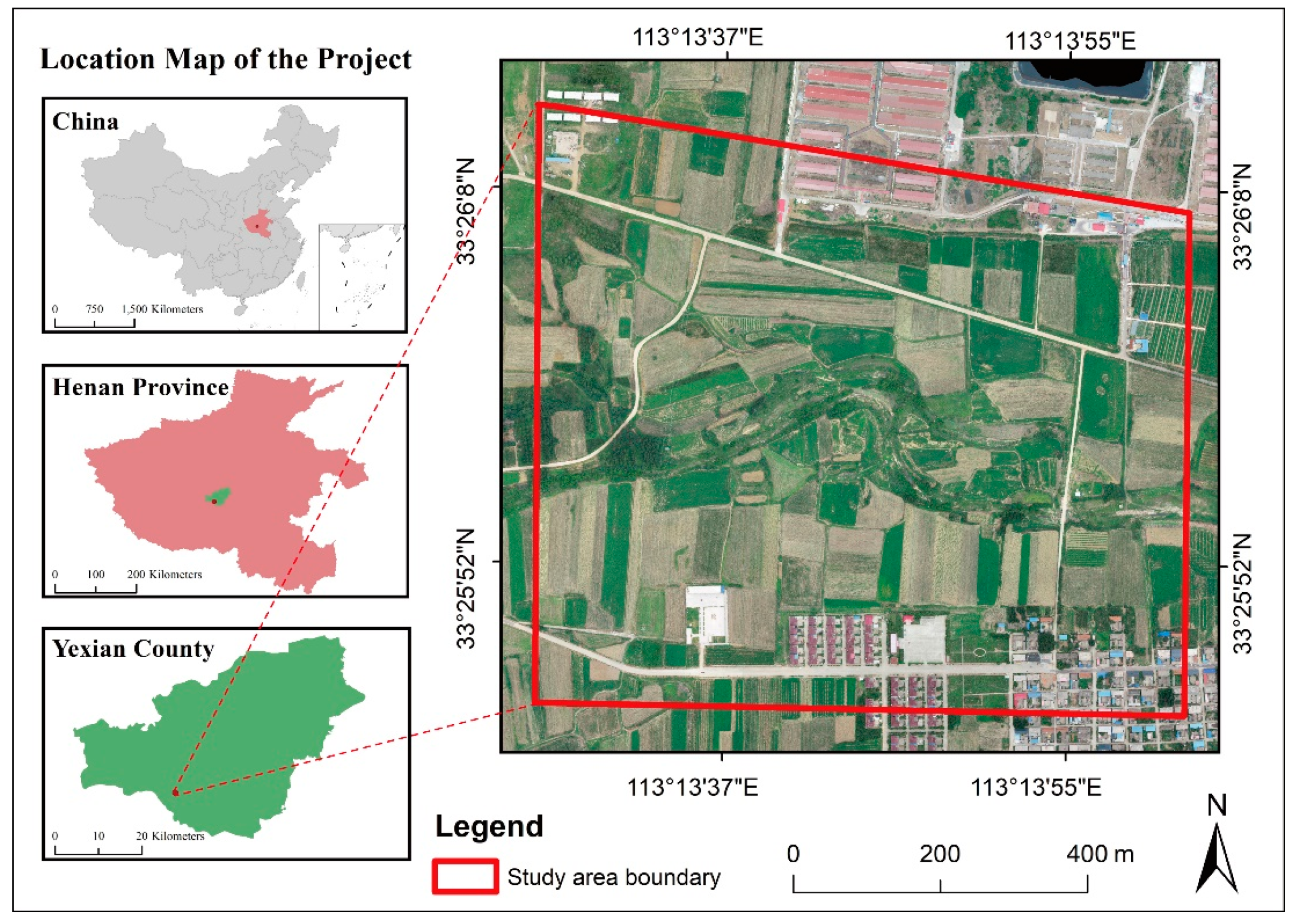
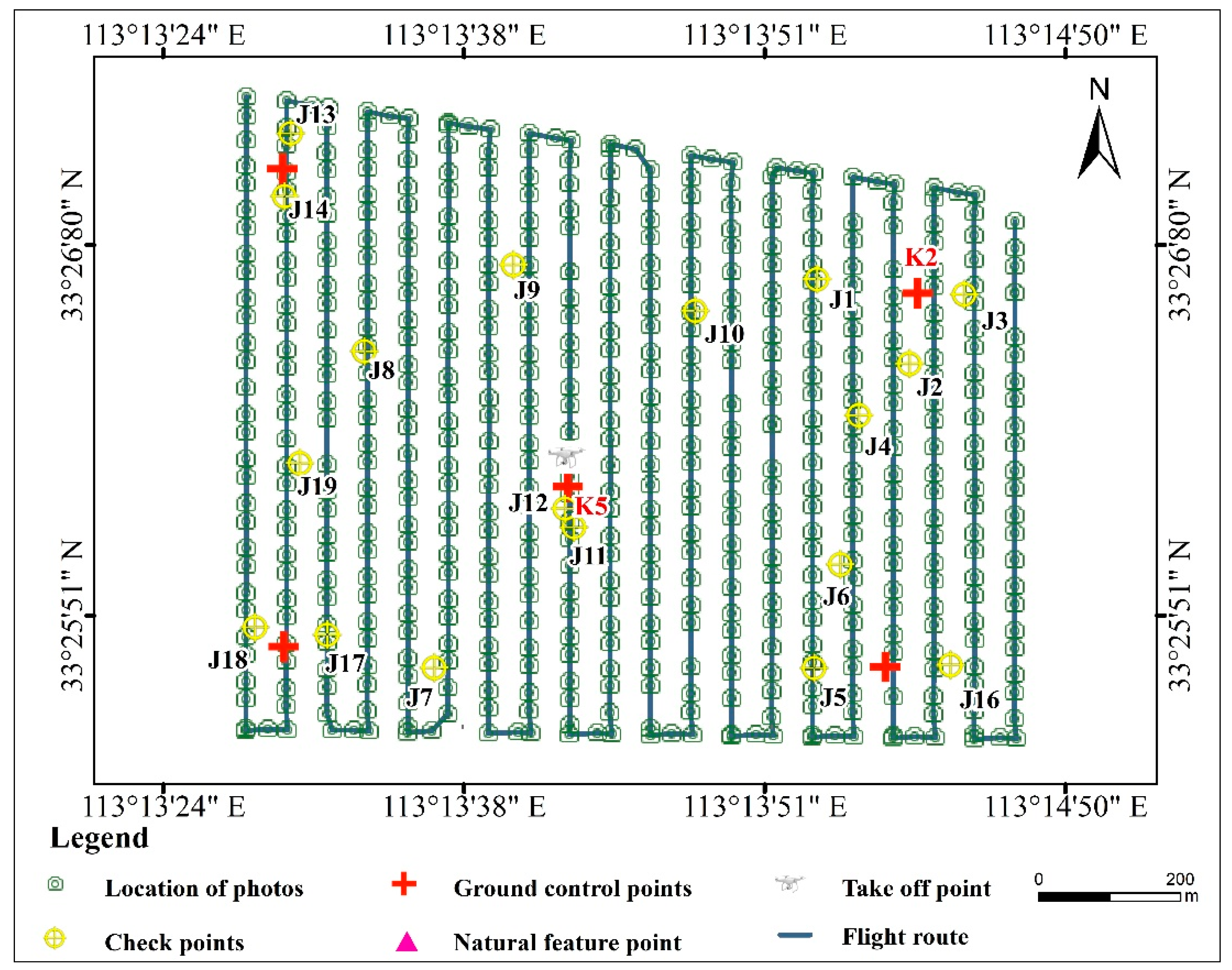
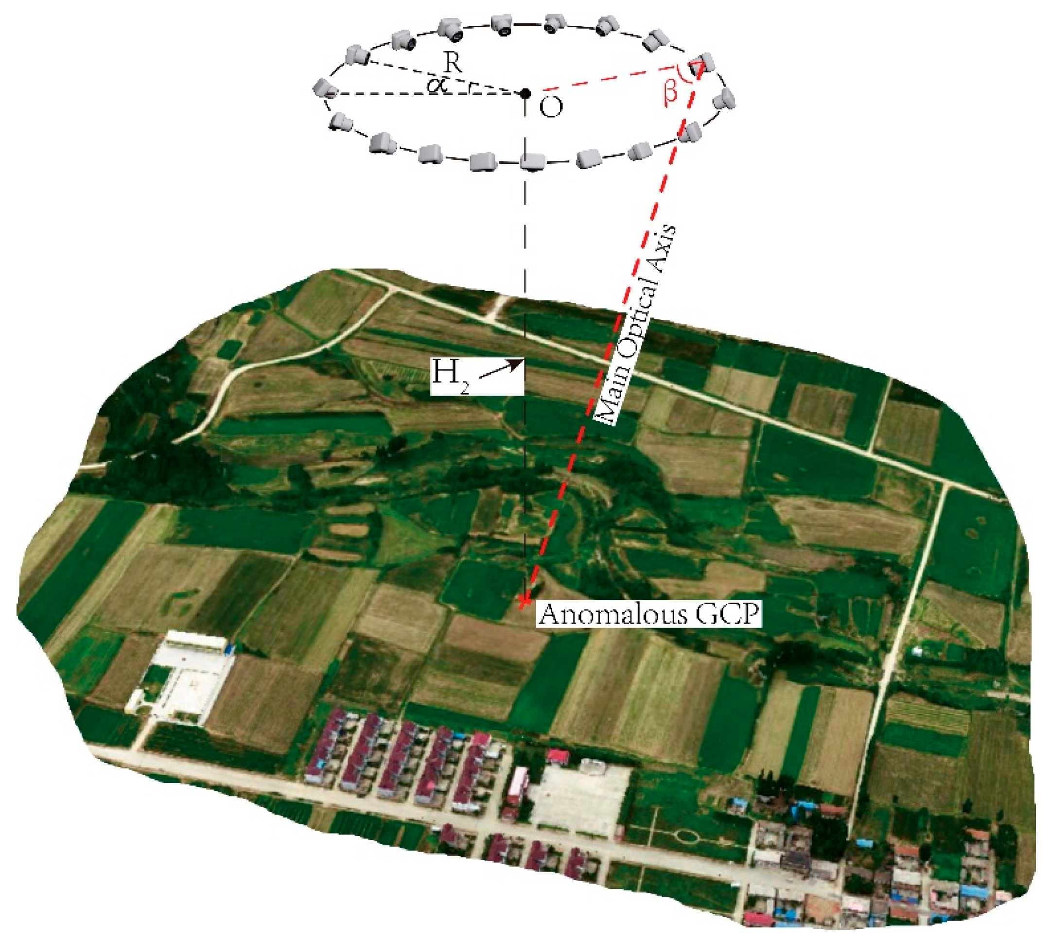
2.1. Study Area

The study area is located in Yanglingzhuang Village, Yexian County, Pingdingshan City, Henan Province, China (Figure 2). The east–west length is about 880 m, the north–south length is about 870 m, and the elevation range is from 154 to 185 m. The longitude range of the study area is 113°13′27″ E~113°14′02″ E, and the latitude range is 33°25′47″ N~33°26′13″ N, with an area of 0.67 km². The study area contains various feature elements, such as arable land, rivers, artificial structures, scrubland, and groves, which are more representative. The wide field of view of the flight and the uninterrupted satellite signal are conducive to collecting images by the UAV.

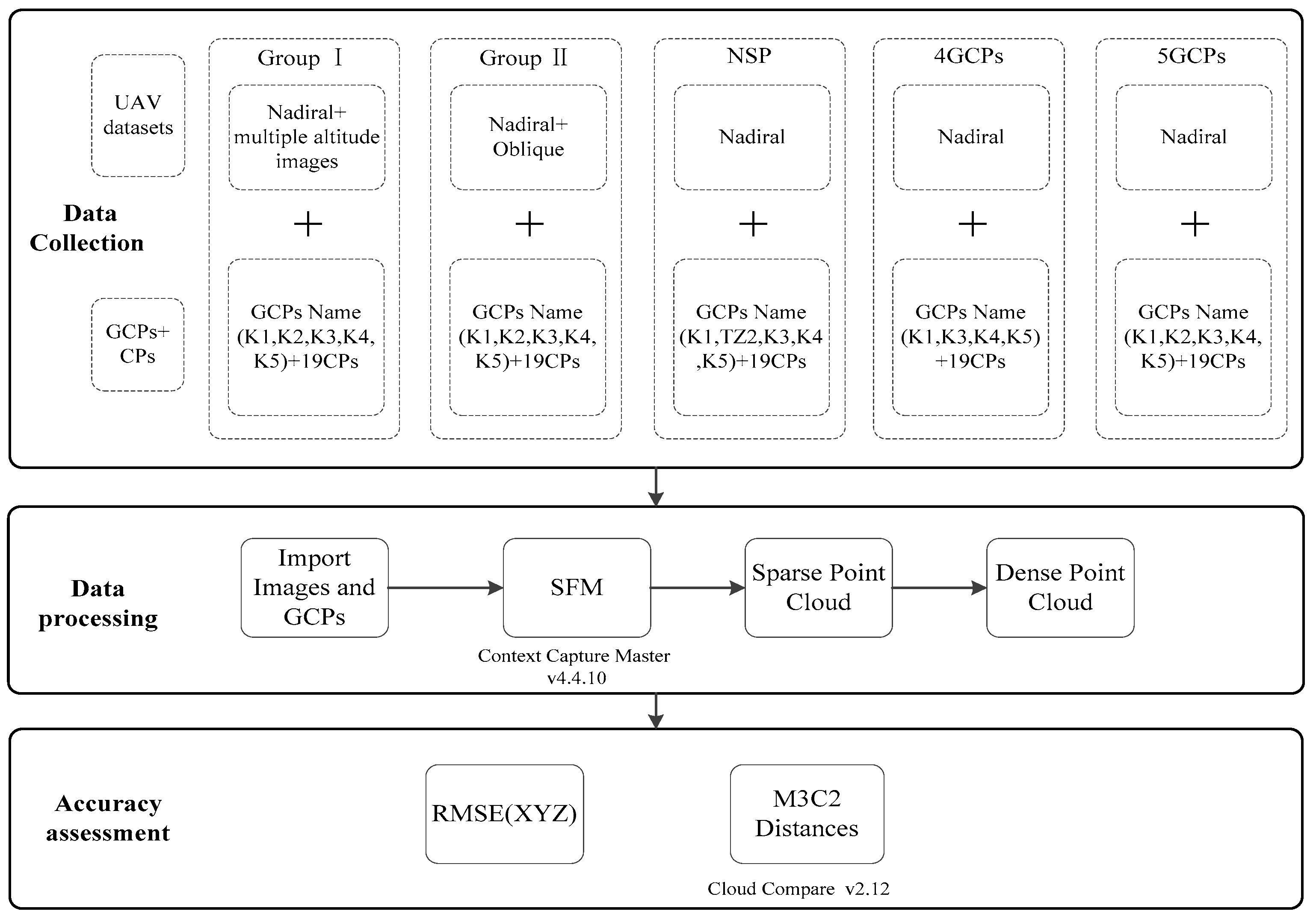
2.2. Overall Workflow

The process of this research (Figure 3) can be divided into three parts, including data acquisition, data processing, and accuracy evaluation. Our proposed solution and the comparison scheme are processed separately by structure from motion (SFM) and multiview stereopsis (MVS), and the results of the different schemes are evaluated for accuracy after the point clouds are generated. The main evaluation metrics include RMSE and M3C2 distance.

There is often a time lag between the placing of GCPs and UAV operations in UAV photogrammetry. During this time gap, GCPs are prone to be vandalised or covered by foreign objects. These problems are not easily detected during the flight of the UAV route, resulting in a reduced availability of the images due to that anomalous GCPs. In order to solve the problem of anomalous GCPs, we proposed two methods called the “STNG” and the “Oblique and Circle”.

“STNG” is a method of taking photographs by descending equidistantly and vertically from sky to near-ground (Figure 4). We defined a specific altitude, H₁, directly above the restored GCP as the starting point (H₁ = H + Δh, where H is the orthometric altitude and Δh is the difference between the altitude of the orthometric take-off point and the altitude of the anomalous control point). We then hovered at certain intervals D to take pictures during the vertical downward movement of the UAV until it reached the surface to complete the operation.

“Oblique and Circle” is a method of surround photography that maintains the oblique angle of the camera for anomalous GCP (Figure 5). We defined that the position of H₂ (same as H₁) directly above the repaired GCP was the centre O, a certain distance R was the radius to make a circular motion, and the camera was inclined at a certain angle β. The heading angle α was a fixed interval to take images. The main optical axis of the camera was required to align with the GCP.

2.3. Data Collection

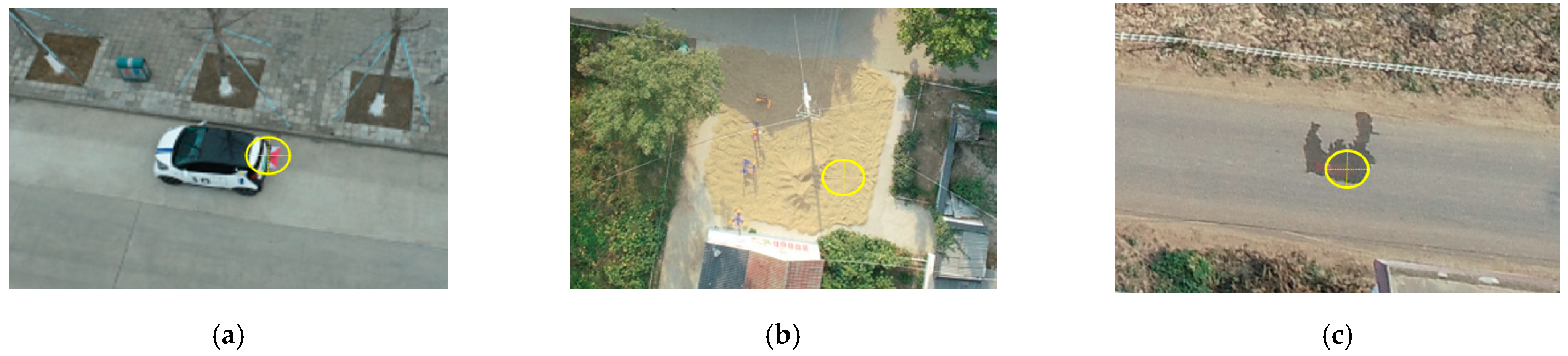
2.3.1. GNSS Survey

According to the characteristics of the field to be studied, we used four corner points combined with a central point to place a total of five GCPs [34]. In order to assess the accuracy, the checkpoints were placed evenly over the study area with a total of 19 CPs (Figure 6). In addition, we searched for the ground natural feature point (the corner point of the bridge named TZ2) near point K2 as a GCP instead of point K2. As the study area is located in the countryside, with more cultivated land and abundant natural landforms, we compared several locations. Finally, we chose the bridge corner point with a high level and more flat terrain as the natural feature point. Two materials were used to place the GCPs and CPs, i.e., pulverized lime for the dirt roads and red paint for the concrete roads.

Three measurements of 24 artificial GCPs and one natural feature point were made in CORS mode using a Huace i80 GNSS receiver. The spatial reference was the CGCS 2000 ellipsoid, the projection was the Gauss—Kruger projection, and the elevation datum was “National Vertical Datum 1985”—all in metres (m). Each positioning was verified to be above 12 satellites, with 10 ephemerides collected each time. The device achieved a horizontal accuracy of ±(8 + 0.5 × 10⁻⁶ × D) mm and a vertical accuracy of ± (15 + 0.5 × 10⁻⁶ × D) mm in CORS mode.

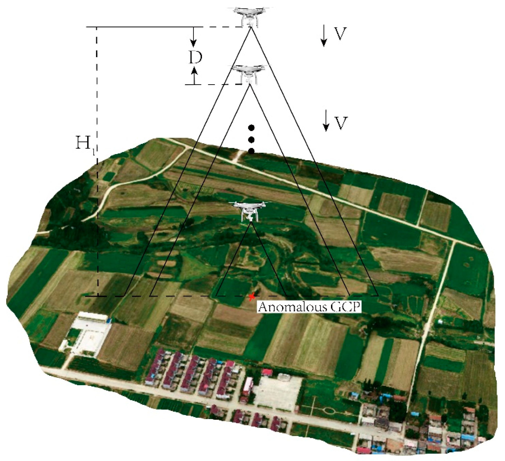
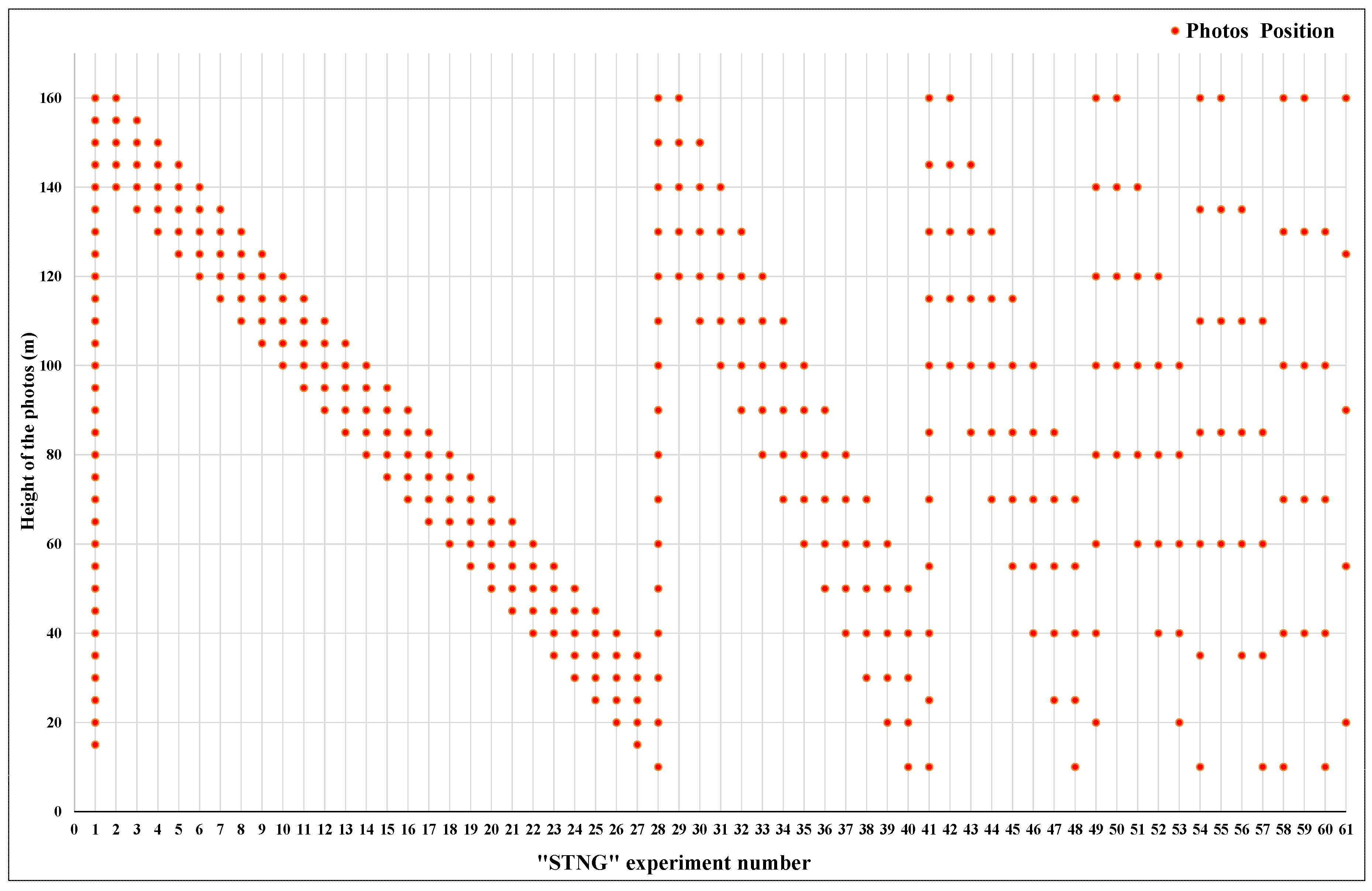
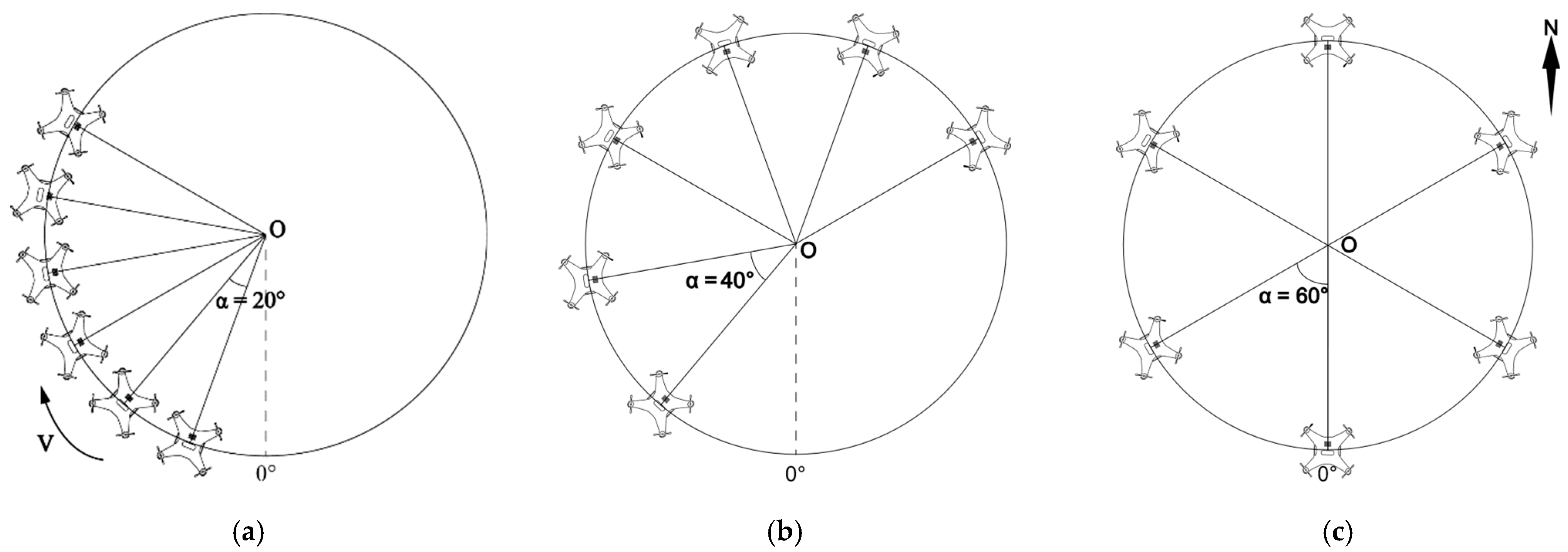
2.3.2. UAV Image Acquisition

The photographs for this experiment were collected using a DJI Phantom 4 Pro drone manufactured by DJI. It is a consumer-grade UAV that is portable, flexible, small in weight and low in cost. It carries a DJI FC6310 camera with a field of view (FOV) of 84° and an image size of 5472 × 3648 pixels. The route planning software used for the experiment was DJI Pilot and DJI GO4. The study area boundary was converted to KML format and imported into DJI Pilot software, the flight altitude (H) above the ground was set to 160 m, the forward overlap was 80%, the side overlap was 80%, the Mapping Mode was set, and the take-off point was selected as point K5 (the altitude of this point is 159.8 m). The camera parameter settings (ISO and exposure values, etc.) are automatically adjusted according to the actual brightness of the scene at the time of flight. The experiment was completed on 4 July 2021 with a light breeze and good light at the site. We collected a total of 562 nadiral images with an average ground resolution of 4.32 cm/pixel. The route and images are shown in Figure 6.

After the nadiral images were acquired, the anomalous GCP was photographed using the method proposed in this paper. As the anomaly GCP (K2) was at the same altitude as the ortho take-off point (K5), the starting flight altitude above the ground for data collection was 160 m (nadiral flight altitude), and then hovered every 5 m down to take one photo for a total of 32 images. The DJI GO4 software was used to complete the data acquisition and determine the height of descent based on the value shown on the display.

We used the DJI GO4 software´s Point of Interest (POI) function while manually controlling the shutter to take photos. The flight altitude above the ground was 160 m, the circle´s centre was O₁, the radius (R) was 20 m, the camera oblique angle was β = 78°, and the heading angle sampling interval α was 20°, meaning that a total of 18 images were acquired. In addition, we added two sets of routes with a flight altitudes of 140 m and 180 m. The parameters for the “oblique and circle” images acquisition are shown in

Table 1. UAV “Oblique and Circle” images acquisition parameters.

Project	Max. Flight Altitude (m)	Radius (m)	Camera Oblique Angle β (°)	Heading Angle Interval α (°)	Number of Images
Flight 1	160	20	78	20	18
Flight 2	140	20	77	20	18
Flight 3	180	20	83	20	18

.

2.4. Data Processing

ContextCapture software is an excellent professional-grade mapping data processing software from Bentley, which can quickly generate real-scene 3D models based on photographs with a certain degree of overlap and output high-precision mapping products, such as TDOM, DSM, and photogrammetric point clouds [35]. It has a robust computer geometry algorithm, an excellent human–computer interface, and is highly operable. We imported the UAV images with various optional additional auxiliary data (camera properties (focal length, sensor size, master point, etc.), photo location information) into the software, used the GCPs for directional aerial triangulation, and then reconstructed it in 3D to obtain a high-resolution triangulated mesh model with realistic textures and a mapping product with a certain degree of accuracy. The software is widely used in China to research and produce topographic products and has a large user base. ContextCapture Center version 4.4.10 was chosen for this experiment to process the data.

The experimental group of “STNG” was named group I; the experimental group of “Oblique and Circle” was named group II. If the K2 point was anomalous, a natural feature point was found as a control point, called “NFP”; four GCPs (K1, K3, K4, and K5) were used to simulate the loss of K2, which was called “4 GCPs”; five GCPs (K1, K2, K3, K4, and K5) were used (K2 is not lost) as the baseline accuracy, which was called “5GCPs”.

Table 2. Overall experiment.

Experiment Name	Description of the Method	Number of GCPs and CPs
Group I	Use “STNG”	5 GCPs + 19 CPs
Group II	Oblique and circle	5 GCPs + 19 CPs
Natural feature point (NFP)	Natural feature point used as GCP (replace K2 Point)	5 GCPs (include 1 NFP) + 19 CPs
4 GCPs	Lose K2 Point	4 GCPs + 19 CPs
5 GCPs	All GCPs are normal	5 GCPs + 19 CPs

shows the detailed description of the overall experiment.

In each experiment in Group I and Group II, “NFP”, “4 GCPs”, and “5 GCPs” were subjected to aerial triangulation operations, and all experiments were performed using uniform parameters (

Table 3. Aerial triangulation parameter setting.

Aero Triangulation Setting	Value
Positioning mode	Use control points for adjustment
Key point density	Normal
Pair selection mode	Default
Component construction mode	OnePass
Tie points	Compute
Position	Compute
Rotation	Compute
Photogroup estimation mode	MultiPass
Focal length	Adjust
Principal point	Adjust
Radial distortion	Adjust
Tangential distortion	Adjust
Aspect ratio	Keep
Skew	Keep

). The number and distribution of checkpoints were consistent for all experiments. To reduce the influence of “human factors”, georeferenced artificial markers at the same locations (pixel coordinates) were used in all experiments [36]. It should be emphasised that due to our flight altitude above the ground of 160 m and the motion blur phenomenon, the location of natural feature points were found in the images as closely as possible [37].

For group I, the main problems we addressed are as follows: firstly, the effect of different distances between adjacent images on accuracy; secondly, the relationship between the variation of its overall (five images) spatial position and accuracy when the image spacing is fixed. Therefore, we set the spacing between adjacent images to 5 m, 10 m, 15 m, 20 m, 25 m, 30 m and 35 m in 7 groups of 61 experiments. There were twenty-seven experiments in the “5 m” group, thirteen experiments in the “10 m” group, eight experiments in the “15 m” group, five experiments in the “20 m” group, four experiments in the “25 m” group, three experiments in the “30 m” group and one experiment in the “35 m” group. The first project for each group was to involve aerial triangulation of all photographs at the corresponding interval. For example, for the “10 m” group, 16 photographs were taken for the first experiment ([10–160 m]), and for the “20 m” group, eight photographs were taken for the first experiment ([20–160 m]). Figure 7 shows the photo participation for each of the experiments.

In Group II, the following two issues were discussed: firstly, the effect on accuracy was explored by varying the flight altitude (140 m, 160 m, 180 m) (Figure 8); secondly, after the optimal flight altitude was obtained, further experiments were completed on the 16 photographs taken at that flight altitude, and 6 of the 16 photographs were selected according to the heading angle interval to explore the effect of the spatial position of the photographs on the accuracy was investigated. The six photographs were selected according to the heading angle interval (20°, 40°, 60°), and six consecutive aerial photographs were taken, respectively (Figure 9).

A set of experimental data was selected from the results of Group I and Group II, respectively, together with the remaining experiments, including “NFP”, ”4 GCPs”, and “5 GCPs” for a total of five experiments. The photogrammetric point cloud model was generated for each experiment, and the sampling distance of the point cloud was set to 0.1 m.

The point cloud analysis was carried out using the M3C2 plug-in of Cloud compare software. The parameters were adjusted according to the system recommended values (Guess params), with a projection radius of 0.87 m, an initial value of 0.44 m, a step size of 0.44 m, a final value of 1.74 m, and a calculation depth of 0.40 m. By comparing the point cloud of each scenario with the reference point cloud data, the overall analysis was carried out on the accuracy of the point cloud data. To improve the reliability of the experimental method, we obtained a set of high-precision reference point clouds by adding GCPs [27]. We increased the number of control points from 5 to 15 to enhance the four corner points and the central point [38].

2.5. Accuracy Assessment

In photogrammetry projects, checkpoints (CPs) are often used to assess accuracy, using the Root Mean Square Error (RMSE) [39,40,41]. After aerial triangulation was completed using ContextCapure software, a quality report was automatically generated, and the RMSE of the CPs were calculated by comparing the CPs coordinates calculated from aerial triangulation with the precise coordinates from the GNSS survey to obtain the RMSE_X, RMSE_Y, and RMSE_Z of the CPs. The detailed equations are given in (1)–(4).

$$RMS{E}_X=\sqrt{\frac{{{\displaystyle \sum }}_{i=1}^n{\left(X_i-X_{GNSSi}\right)}^2}{n}}$$

(1)

$$RMS{E}_Y=\sqrt{\frac{{{\displaystyle \sum }}_{i=1}^n{\left(Y_i-Y_{GNSSi}\right)}^2}{n}}$$

(2)

$$RMS{E}_Z=\sqrt{\frac{{{\displaystyle \sum }}_{i=1}^n{\left(Z_i-Z_{GNSSi}\right)}^2}{n}}$$

(3)

$$RMS{E}_{XY}=\sqrt{\frac{{{\displaystyle \sum }}_{i=1}^n{\left(X_i-X_{GNSSi}\right)}^2+{\left(Y_i-Y_{GNSSi}\right)}^2}{n}}$$

(4)

where n is the number of CPs; X_GNSSi, Y_GNSSi, Z_GNSSi are the X, Y, Z actual geographic coordinates of the i-th CP measured by GNSS, respectively; X_GNSSi, Y_GNSSi, Z_GNSSi are the X, Y, Z actual geographic coordinates of the i-th CP measured by GNSS, respectively.

For an overall accuracy comparison, we generated photogrammetric point clouds from the different scenarios and used CloudCompare 2.12 software point clouds for comparison [42]. The primary use of the Multiscale Model to Model Cloud Comparison (M3C2) plug-in is one of the more widely used ways to evaluate distance calculation methods for 3D change features [43]. In M3C2, a set of highly accurate and precise point cloud data was used as a reference, and the distance in the direction of the normal to the local surface was calculated for the reference and comparison point clouds by using two parameters (custom normal scale and projection scale). The accuracy and precision of the point cloud data were assessed using the mean value and Standard Deviation (std.dev), respectively. By plotting the errors and their distribution curves, we determined the spatial distribution of the M3C2 distances for the different experiments, thus completing the error assessment [44].

3. Results

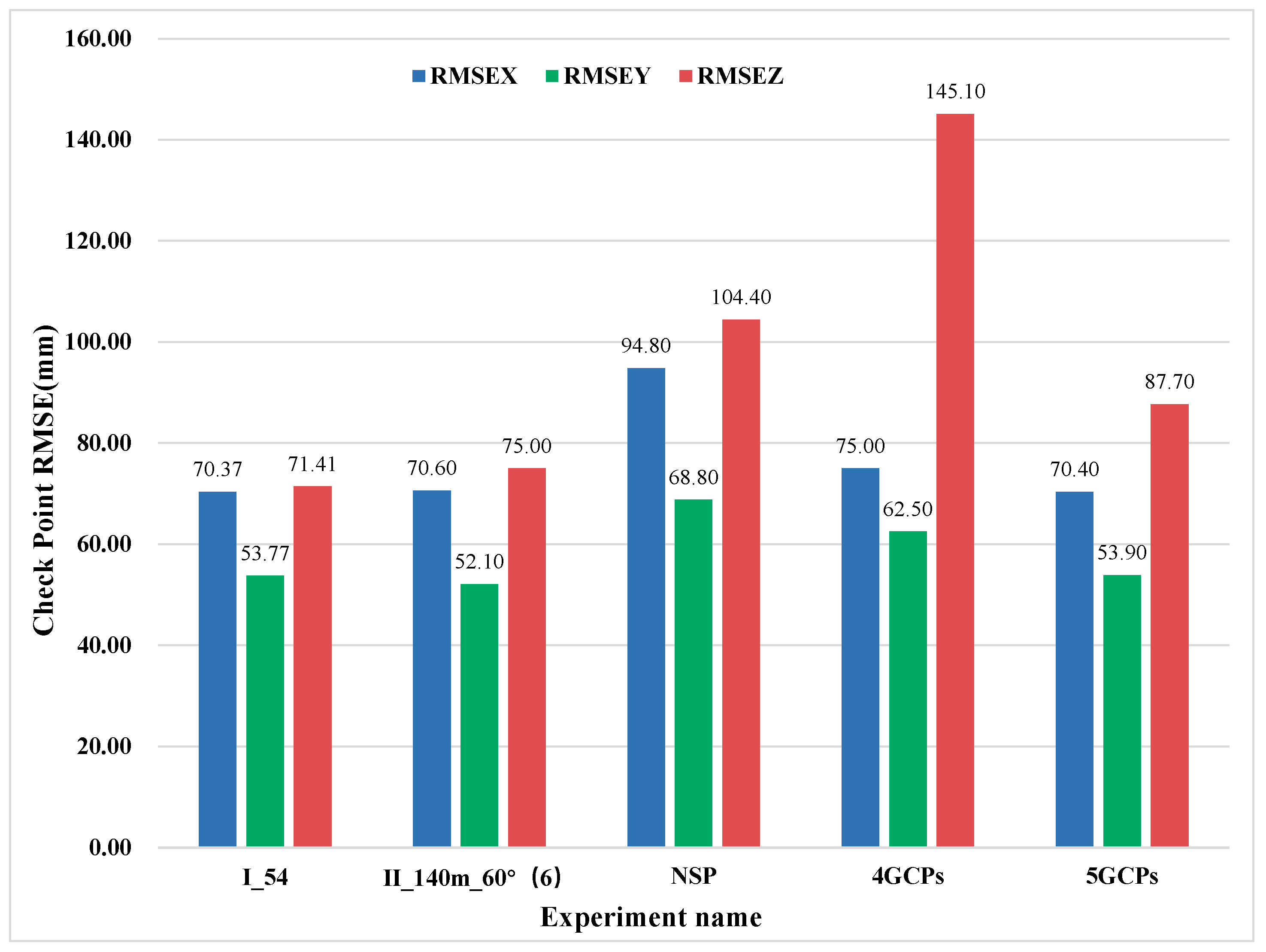
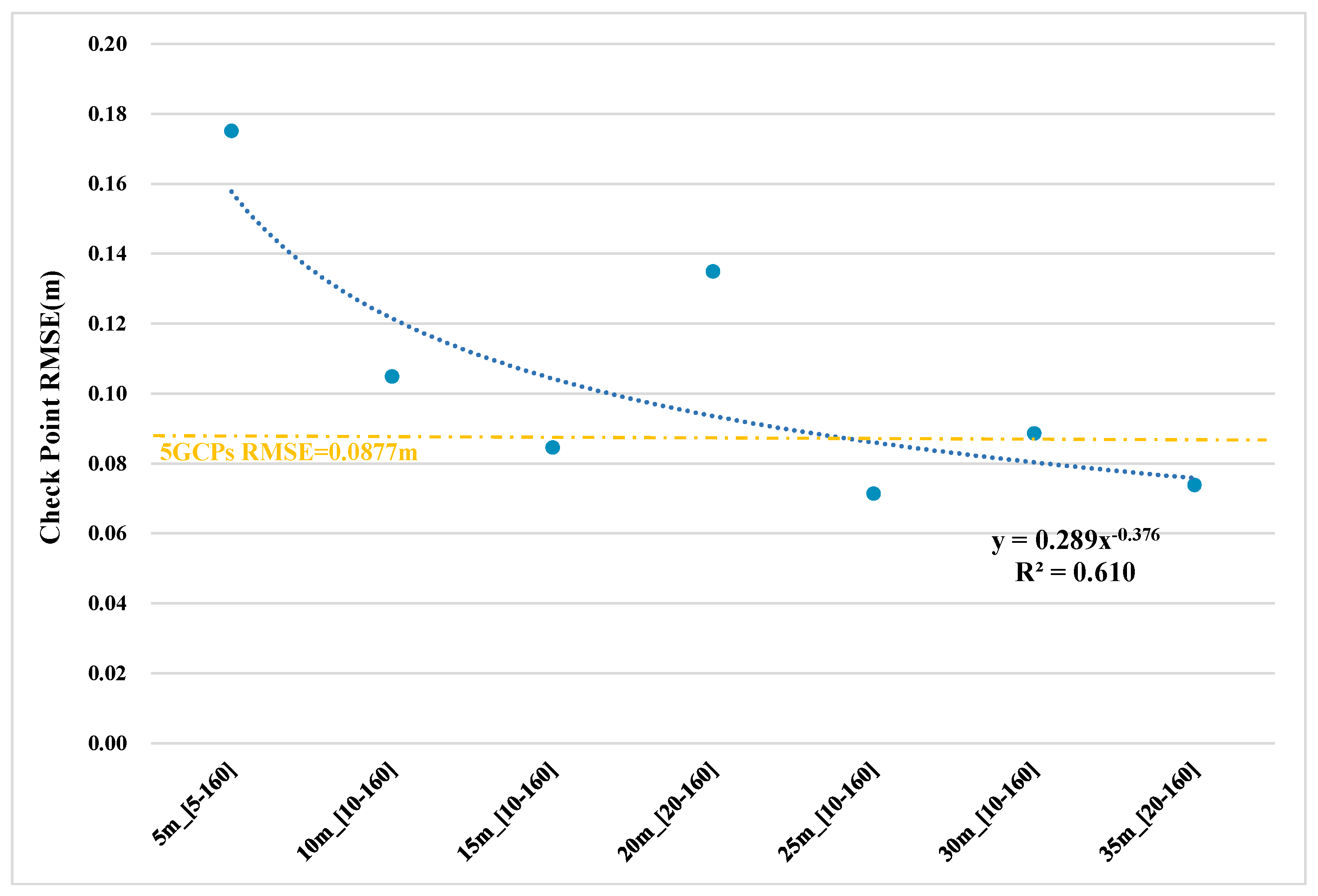
3.1. Accuracy Based on RMSE

In Group I, we used the sampling interval of the photographs as a variable for a total of 61 experiments. We evaluated the accuracy of all the experiments to obtain the error values of all CPs in the plane and elevation directions for each experiment and the RMSE_X, RMSE_Y, and RMSE_Z of the CPs for each experiment. In Figure 10a, the overall planimetric error of the CPs of group I converges to 0.2 m, which is relatively stable. It is evident that the curves of CPs (J1, J2, and J3) are steeper and have more significant Measures of Dispersion compared with the rest of the CPs. The errors of J1, J2, and J3 in different experiments in group I differ greatly, while J1, J2, and J3 are distributed around the GCP K2, which indicates that the “STNG” method had a greater impact on the local accuracy. However, the absolute error of the CPs of each experiment is small, and the overall planimetric error is very stable.

Figure 10 shows that the distribution of error values in the elevation direction is not as concentrated as the plane, and the overall convergence was −0.5 m~0.2 m. There are apparent differences in the elevation errors between the different experiments in group I, which was unstable. The instability of CPs (J1, J2, J3, J4, and J10) is more pronounced, as these 5 points were distributed around K2, further verifying that the “STNG” method has a greater impact on local accuracy. On the other hand, the crests indicate the convergence of error values for the overall CPs of this experiment, and elevation errors were smaller. It can be found that the experiments in the case of full photo participation (experiment numbers 1, 28, 41, 49, 54, 58, and 61) are at the wave crest in the group of seven different sampling interval distances; this means that a uniform distribution of photographs within 160 m according to the sampling interval has less error than a partial take of five, while the number of uniformly distributed photographs is greater compared to five (five photos for 35 m sampling distance). Figure 11 represents the fitted curve between sampling interval and CPs RMSE for these seven experiments. The results show that the effect of the sampling interval on the CPs was significant, with the RMSE of the CPs gradually decreasing and then stabilising as a power function relationship as the distance between the sampling intervals increases (regression coefficients R² = 0.610, significance level p < 0.05). However, larger sampling intervals (40 m and above) would not satisfy the experimental conditions, which were limited by the flight height of the data itself.

In order to determine how the accuracy varies with the spatial position of the photograph in the vertical direction, a correlation analysis was carried out on the “5 m” series of 26 experiments. The experiments are numbered 2–27 (Figure 7) (remove experiment number 16, which has a large outlier, RMSE_Z = 0.0815 m). Figure 12 shows a significant correlation between the overall height of the five photographs and the CPs RMSE_Z, with the RMSE_Z showing a linear increase as the overall height of the photographs increases (regression coefficients R² = 0.6434, Pearson coefficient of 0.811, significance level p < 0.001). The values in the graph are valid only for this study, as the errors depend on the sampling interval.

The main focus of Group II was to investigate the effect of different flight altitudes and heading angle intervals on accuracy. In the nomenclature of the experiment, II_140 m_20° (18) indicates an “Oblique and Circle” of 18 photographs at a flight height of 140 m and a heading angle interval of 20°.

Table 4. RMSE in the horizontal and elevation direction for different flight altitudes and different numbers of photographs using the “Oblique and Circle” method.

Experiment	RMSEX (mm)	RMSEY (mm)	RMSEZ (mm)
II_140m_20° (18)	70.70	51.80	77.90
II_140m_60° (6)	70.60	52.10	75.00
II_160m_20° (18)	71.10	51.10	87.30
II_160m_60° (6)	71.30	50.70	83.00
II_180m_20° (18)	70.80	50.80	74.30
II_180m_60° (6)	70.30	53.20	84.20

shows the RMSE of the CPs for the different solutions of the “Oblique and Circle” method. Different schemes can meet the accuracy requirements of “5GCPs” (RMSE_X = 70.40 mm, RMSE_Y = 53.90 mm, RMSE_Z = 87.70 mm) in both horizontal and elevation directions, indicating the effectiveness and stability of the “Oblique and Circle” method. When the number of images was reduced to six, the overall accuracy does not change significantly, so we preferred to use six images. After comparison, the 140 m aerial height shows a higher elevation accuracy, with the best being at CPs RMSE_Z = 75 mm.

From the results of the above experiments, it can be concluded that the accuracy was better at a flight altitude of 140 m. Therefore, data with a flight altitude of 140 m was used to explore the effect of different spatial positions of the photographs on accuracy. The number of photographs was six, and three sets of experiments were designed (Figure 9). The results of the experiments are shown in

Table 5. CPs RMSE of three distribution modes at 140 m altitude by the “Oblique and Circle” method.

Experiment	RMSEX (mm)	RMSEY (mm)	RMSEZ (mm)
II_140m_60° (6)	70.60	52.10	75.00
II_140m_20° (6)	71.00	51.90	79.80
II_140m_40° (6)	70.50	52.50	86.00

. The errors show fluctuations as the relative spatial positions of the photographs vary. The smallest error is in experiment II_140m_60° (6), representing a uniform distribution of images, with the heading angle of every two images differing by 60° and the RMSE_Z being 75 mm. However, the RMSE_Z for the rest of the experiments was less than 87.70 mm (5 GCPs), which further validates the stability of the “Oblique and Circle” method.

Experiment I_54 and experiment II_140m_60° (6) were used as the representative results of group I and group II, respectively, and the accuracy was compared with “NFP” (using natural feature points as control points), “4 GCPs” (K2 point loss), and “5 GCPs”. From Figure 13, in the X-direction, the largest error was NFP with CPs RMSE_X = 94.80 mm, followed by 4 GCPs, CPs RMSE_X = 75 mm. The results show that adding a natural feature point as a GCP did not improve the accuracy but reduced it to some extent. The RMSE_X of Experiment I_54, Experiment II_140 m_60° (6), and 5 GCPs were 70.37 mm, 70.60 mm, and 70.40 mm, respectively, and the accuracy in the X-direction remained the same for all three. The error distribution pattern in the Y-direction is consistent with that in the X-direction. It is verified that our methods can meet the requirements of 5GCPs accuracy in the horizontal direction.

In the Z-direction of elevation, the four GCPs exhibited the largest error, with CPs RMSE_Z = 145.10 mm being greater than the 5 GCPs (CPs RMSE_Z = 87.70 mm), which indicates that the absence of a GCP has a greater impact on the overall elevation accuracy. The NFP solution RMSE_Z was 104.40 mm, which is between 4 GCPs and 5 GCPs, indicating that the addition of a natural feature point can improve the overall accuracy to some extent, compared to the elevation accuracy of 4 GCPs, but cannot achieve the accuracy (5 GCPs). In contrast, both the “STNG” and the “Oblique and Circle” met the accuracy of the 5 GCPs with an CPs RMSE_Z of 71.41 mm and 75.00 mm, respectively, to a certain extent, thus improving the elevation accuracy.

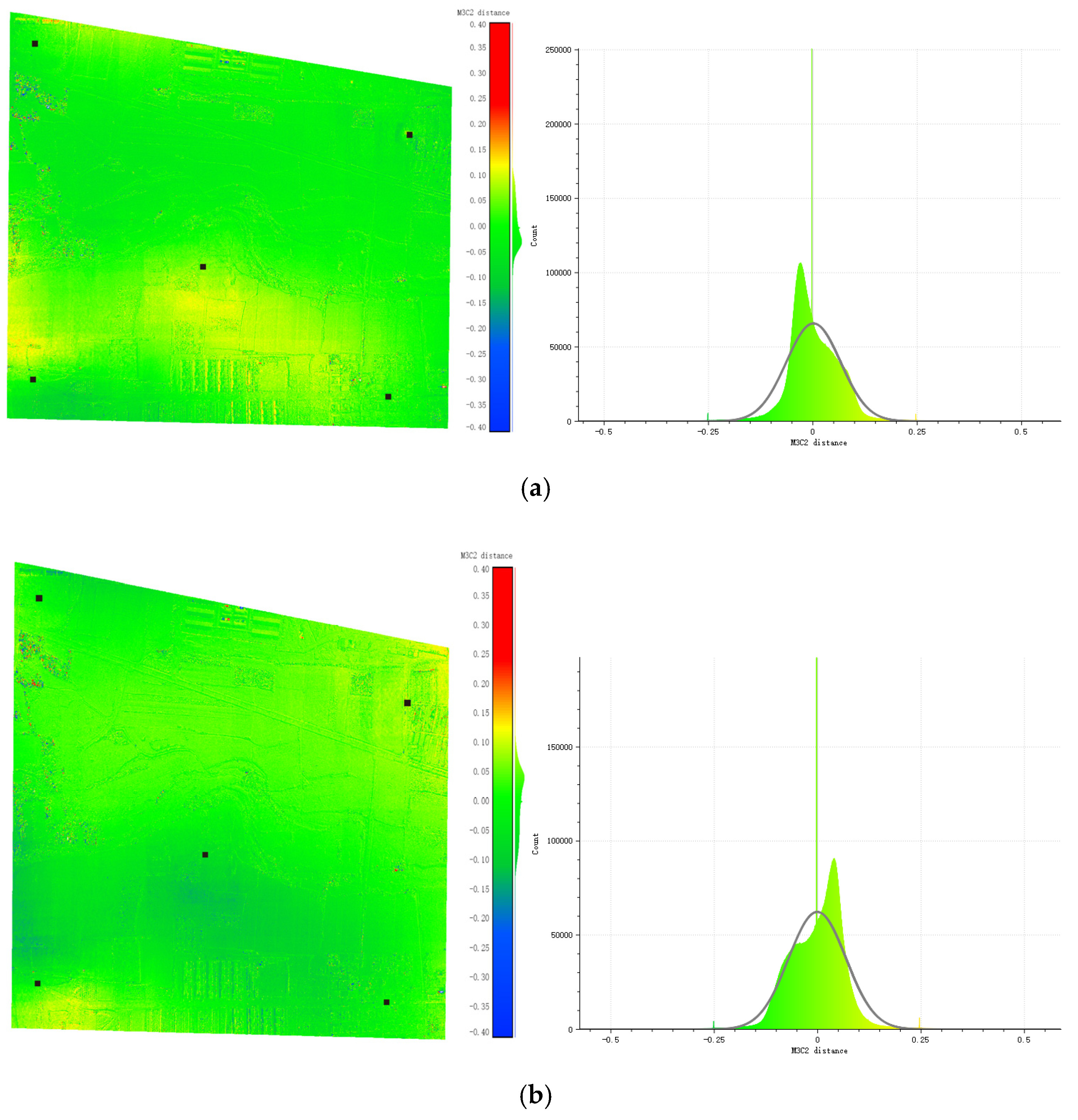
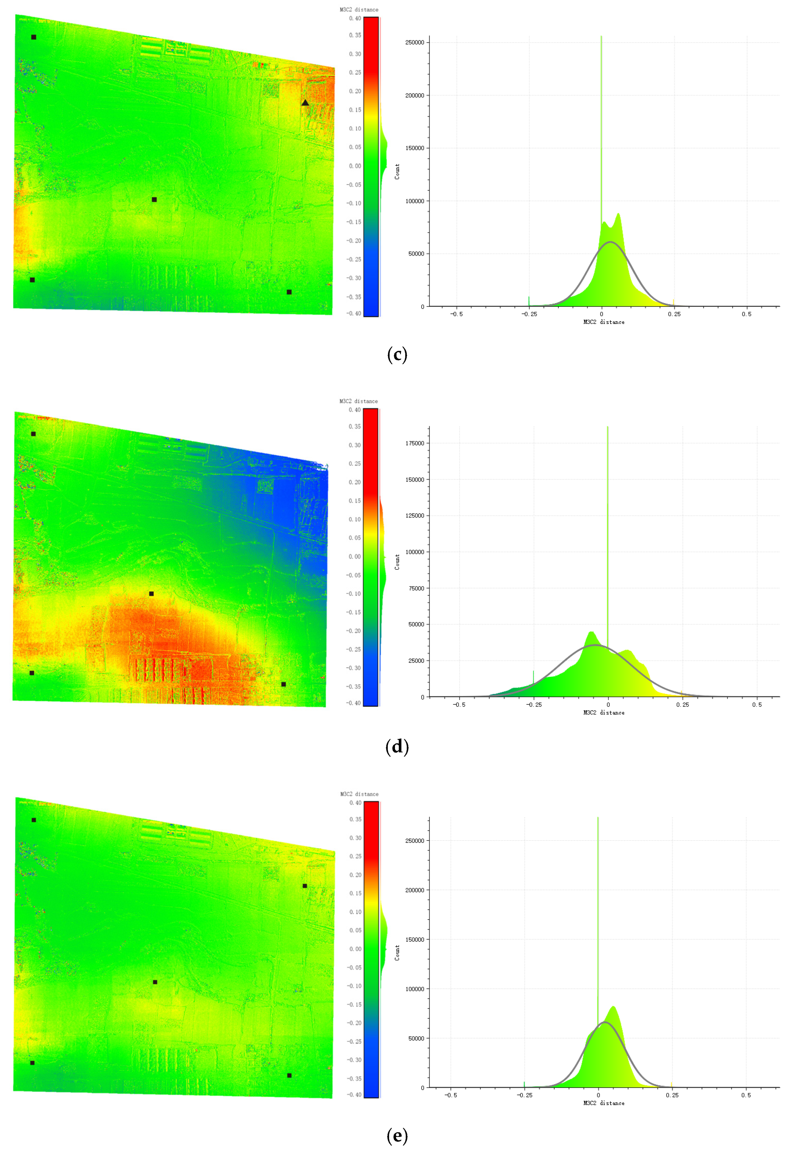
3.2. Point Cloud Evaluation Based on M3C2 Distance

The photogrammetric point cloud of the “15 GCPs” scheme was used as the reference point cloud, and the M3C2 distance operation was performed with the above five sets of experimental point clouds respectively, to obtain the point cloud change results (Figure 14). The comparative analysis shows that the”4 GCPs” (mean = −0.0409, std. dev = 0.1223) was greatly affected in terms of accuracy and precision compared to “5 GCPs” (mean = −0.0239, std. dev = 0.0666), and the use of natural feature point as a GCP (mean = −0.0320, std. dev = 0.0734) could improve the accuracy but failed to achieve the 5 GCPs accuracy. When five additional images with different altitudes (I_54) were added (mean = 0.0040, std. dev = 0.0652), the accuracy greatly improved (Figure 14a). When five oblique-circle images (II_140 m_60° (6)) were added (mean = 0.0017, std. dev = 0.0694), the overall accuracy and precision improved significantly and were closer to that of the 15 GCPs (Figure 14b).

When the GCP (K2) is lost, it significantly impacted the accuracy of the study area, especially around the anomalous GCP and houses, which could be improved by the “STNG” and “Oblique and Circle” solution, and was significantly better than the use of natural feature points (Figure 14c).

4. Discussion

We placed GCPs at each of the four corners and central points within the approximately rectangular study area, and this approach was feasible. Both Rangel et al. [45] and Patricio Martínez-Carricondo et al. [46] argued that a uniform distribution around the experimental area and the addition of uniformly distributed GCPs in the middle of the experimental area can improve the elevation accuracy. The errors introduced when a corner point K2 is lost are significant, especially in elevation, with the RMSE_Z of the CPs reaching 145.10 mm compared to the 5 GCPs RMSE_Z = 87.70 mm. Therefore, the quality of the photographs after the loss of a GCP should be questioned and should not be used directly.

The anomalies in GCPs have rarely been discussed in previous studies. The general method of a “natural feature point” has limitations and is very dependent on the quality of the natural feature points and the subjective judgement of the data processor. It was found that when natural feature points were used as control points (NFP scheme), the error in the elevation direction of the CPs reached 104.40 mm, which is not possible to achieve the accuracy of 5 GCPs. There is a significant increase in error in the horizontal direction, with the CPs RMSE_X reaching 94.80 mm compared to the 5 GCPs checkpoints RMSE_X of 70.40 mm, further verifying that NFP is unable to achieve the 5 GCPs’ accuracy in both the horizontal and elevation directions. Such instability is determined by the quality of the natural feature point— its actual position is not easy to find on the aerial images and is often met with some deviation. Francisco-Javier Mesas–Carrascosa’s study shows that instead of using well-defined artificial checkpoints, the use of natural feature points in the study area as checkpoints would increase the checkpoint RMSE from a GSD of 3.7 times to a GSD of five times [47].

The idea of the “STNG” method is to improve the ground resolution of the area around the GCP by progressively taking additional images downwards and fusing them with the nadiral images, thus improving the accuracy. Quoc Long et al. [48] mentioned that increasing the ground resolution by reducing the flight altitude of the UAV could improve the accuracy, and Agüera-Vega et al. [38] showed that the effect of GSD on elevation accuracy was significant. In contrast, the effect on planimetric accuracy was smaller.

It was found that the “STNG” showed high stability in the horizontal direction but less stability in the elevation direction. The first experiment of each group represents the best case for each group, all the images in each group are involved, and their spatial locations are shown in Figure 7. As the interval between adjacent photos increased, the elevation accuracy showed a nonlinear trend of gradual improvement and stability (regression coefficients R² = 0.610, significance level p < 0.05), which is consistent with the accuracy of “5 GCPs”, indicating that the “STNG” is feasible. The best solution is to set the sampling interval as 25 m (I_54), where all seven images were involved and the RMSE_X = 70.37 mm, RMSE_Y = 53.77 mm, RMSE_Z = 71.41 mm of the CPs. The RMSE_Z of the CPs of the sampling interval of 30 m (I_58) and 35 m (I_61) were 88.61 mm and 73.85 mm—both of which met the 5 GCP’s accuracy requirements. Therefore, we suggest that in the actual operation, the sampling interval D should be determined with reference to the nadiral flight altitude ((H + Δh)/7 ≤ D ≤ (H + Δh)/5, where H is the nadiral flight altitude and Δh is the difference between the altitude of the nadiral take-off point and the altitude of the anomalous GCP).

In experiments with a sampling interval of 5 m, we found a linear trend in the accuracy of the data with decreasing photo height (regression coefficients R² = 0.6434, significance level p < 0.001). This observation will need to be verified in further studies.

A total of six experiments were set up in Group II to verify the influence of altitude and number of photographs on the accuracy, and three experiments were set up to verify the influence of different spatial positions of photographs at the same altitude on accuracy. The results show that the accuracy of the 5 GCPs can be achieved at different flight altitudes, indicating that the “Oblique and Circle” method has high stability. The highest elevation accuracy was demonstrated at an altitude of 140 m. The difference between the accuracy of 18 additional images and six images is not significant, so using six images was a better choice. When the spatial position of six images was evenly distributed, and the heading angles of different images were spaced 60° apart, which is more accurate. The horizontal error of the above experiment is about one-to-two times the GSD, and the elevation error is about two-to-three times the GSD, which satisfies the general law of photogrammetry [49].

By using the “Oblique and Circle” method, there is a clear tendency to improve accuracy in the elevation direction further. The RMSE_Z of the CPs of the II_140m_60° (6) experiment is 75.00 mm, which is about 10 mm higher elevation accuracy than the 5 GCPs. Wackrow et al. [50] suggested that the angle between homologous rays could be increased by introducing oblique images in the nadiral dataset, thus reducing systematic errors. Bi et al. [51], Harwin et al. [52], and Štroner et al. [25] have shown that adding additional oblique images to the nadiral images can improve the accuracy of the results and increase the elevation accuracy. Sanz-Ablanedo et al. [53] showed that square POI flights, where the camera angle is always aligned with the centre of the region of interest, produce a smaller systematic error. Therefore, we believe that the “Oblique and Circle” method is valid and is valuable for further research.

The M3C2 point cloud comparison confirms our viewpoint as well. Using the “STNG” and “Oblique and Circle” methods can improve the elevation accuracy to a certain extent while still meeting the 5 GCPs’ accuracy. The “Oblique and Circle” method provides the highest elevation accuracy and is more stable. The “natural feature point” method has a significant local error (Figure 14c), and the overall accuracy is not as good as required.

In UAS, the height above the ground level can be measured based on barometer sensors. The DJI Phantom 4 Pro UAV used in this study has a vertical positioning accuracy of ±0.5 m, which means that height deviations at the decimetre level may occur during data acquisition and that the centimetre level (or smaller) positioning accuracy cannot be accomplished [54]. However, the two methods are experimentally compatible, and the decimetre-level positioning errors have less impact on the two methods. Therefore, the vertical positioning errors of the UAV itself can be ignored when using the methods.

At the same time, the limitations of fixed-wing UAVs make it challenging to use the method proposed in this paper to collect images. Therefore, the fusion of images using different camera sensors is proposed, such as using a more flexible multirotor UAV to complement images; this will be the next stage of our research.

5. Conclusions

In this paper, two different solutions based on ground control point anomalies were put forward, and the optimum of which was verified. By adopting the “5 GCPs” as the reference project and the “NFP” method as the comparison solution, the following conclusions can be drawn.

It is not easy to find natural feature points that meet the requirements outside urban areas. The location of the feature points in the image depends on the subjective judgment of professionals with a large error caused by “human factors”. For this reason, it is not recommended that “natural features” be the preferred option for aerial photogrammetry when high accuracy is required.

In practical projects, only when horizontal accuracy is required, can our proposed “STNG” and “Oblique and Circle” methods meet the accuracy requirements. The “NFP” demonstrates that neither the horizontal nor the elevation direction can meet the requirements of the 5 GCPs’ accuracy. The “STNG” method is simple and easy to use, so it is recommended. When using the “STNG” method, the spacing between the adjacent images is D ((H + Δh)/7 ≤ D ≤ (H+ Δh)/5, where H is the nadiral flight altitude, Δh is the difference between the elevation of the nadiral take-off point and the elevation of the anomaly GCP, and the number of photographs must not be less than 5.).

When elevation accuracy is considered, the “Oblique and Circle” method has higher stability and meets the accuracy requirements. In the horizontal direction, the accuracy is maintained and consistent with the data´s accuracy from the 5 GCPs. There is a tendency to improve the accuracy further in the elevation direction. When using the “Oblique and Circle” method, the accuracy requirements can be met by keeping the flight height the same as the flight height of the nadiral. To improve the elevation accuracy, the flight height can be reduced by a small amount, e.g., about 20 m in the experiment of this paper. At the same time, the selection of photographs should be evenly distributed around the entire circumference, and the results are better when the heading angle is 60°. In sum, the “Oblique and Circle” method is highly effective when the GCPs are anomalous.

References

1. Šafář, V.; Potůčková, M.; Karas, J.; Tlustý, J.; Štefanová, E.; Jančovič, M.; Cígler Žofková, D. The Use of UAV in Cadastral Mapping of the Czech Republic. ISPRS Int. J. Geo-Inf. 2021, 10, 380. [Google Scholar] [CrossRef]
2. Puniach, E.; Bieda, A.; Ćwiąkała, P.; Kwartnik-Pruc, A.; Parzych, P. Use of Unmanned Aerial Vehicles (UAVs) for Updating Farmland Cadastral Data in Areas Subject to Landslides. ISPRS Int. J. Geo-Inf. 2018, 7, 331. [Google Scholar] [CrossRef] [Green Version]
3. Chio, S.-H.; Chiang, C.-C. Feasibility Study Using UAV Aerial Photogrammetry for a Boundary Verification Survey of a Digitalized Cadastral Area in an Urban City of Taiwan. Remote Sens. 2020, 12, 1682. [Google Scholar] [CrossRef]
4. Alexiou, S.; Deligiannakis, G.; Pallikarakis, A.; Papanikolaou, I.; Psomiadis, E.; Reicherter, K. Comparing High Accuracy t-LiDAR and UAV-SfM Derived Point Clouds for Geomorphological Change Detection. ISPRS Int. J. Geo-Inf. 2021, 10, 367. [Google Scholar] [CrossRef]
5. De Marco, J.; Maset, E.; Cucchiaro, S.; Beinat, A.; Cazorzi, F. Assessing Repeatability and Reproducibility of Structure-from-Motion Photogrammetry for 3D Terrain Mapping of Riverbeds. Remote Sens. 2021, 13, 2572. [Google Scholar] [CrossRef]
6. Kyriou, A.; Nikolakopoulos, K.; Koukouvelas, I. How Image Acquisition Geometry of UAV Campaigns Affects the Derived Products and Their Accuracy in Areas with Complex Geomorphology. ISPRS Int. J. Geo-Inf. 2021, 10, 408. [Google Scholar] [CrossRef]
7. Bakirman, T.; Bayram, B.; Akpinar, B.; Karabulut, M.F.; Bayrak, O.C.; Yigitoglu, A.; Seker, D.Z. Implementation of Ultra-Light UAV Systems for Cultural Heritage Documentation. J. Cult. Herit. 2020, 44, 174–184. [Google Scholar] [CrossRef]
8. Berrett, B.E.; Vernon, C.A.; Beckstrand, H.; Pollei, M.; Markert, K.; Franke, K.W.; Hedengren, J.D. Large-Scale Reality Modeling of a University Campus Using Combined UAV and Terrestrial Photogrammetry for Historical Preservation and Practical Use. Drones 2021, 5, 136. [Google Scholar] [CrossRef]
9. Teppati Losè, L.; Chiabrando, F.; Giulio Tonolo, F. Documentation of Complex Environments Using 360° Cameras. The Santa Marta Belltower in Montanaro. Remote Sens. 2021, 13, 3633. [Google Scholar] [CrossRef]
10. Fraser, B.T.; Congalton, R.G. Estimating Primary Forest Attributes and Rare Community Characteristics Using Unmanned Aerial Systems (UAS): An Enrichment of Conventional Forest Inventories. Remote Sens. 2021, 13, 2971. [Google Scholar] [CrossRef]
11. Malachy, N.; Zadak, I.; Rozenstein, O. Comparing Methods to Extract Crop Height and Estimate Crop Coefficient from UAV Imagery Using Structure from Motion. Remote Sens. 2022, 14, 810. [Google Scholar] [CrossRef]
12. Pagliai, A.; Ammoniaci, M.; Sarri, D.; Lisci, R.; Perria, R.; Vieri, M.; D’Arcangelo, M.E.M.; Storchi, P.; Kartsiotis, S.-P. Comparison of Aerial and Ground 3D Point Clouds for Canopy Size Assessment in Precision Viticulture. Remote Sens. 2022, 14, 1145. [Google Scholar] [CrossRef]
13. Santana, L.S.; Ferraz, G.A.e.S.; Marin, D.B.; Faria, R.d.O.; Santana, M.S.; Rossi, G.; Palchetti, E. Digital Terrain Modelling by Remotely Piloted Aircraft: Optimization and Geometric Uncertainties in Precision Coffee Growing Projects. Remote Sens. 2022, 14, 911. [Google Scholar] [CrossRef]
14. Albeaino, G.; Gheisari, M. Trends, benefits, and barriers of unmanned aerial systems in the construction industry: A survey study in the United States. J. Inf. Technol. Constr. 2021, 26, 84–111. [Google Scholar] [CrossRef]
15. Esposito, G.; Mastrorocco, G.; Salvini, R.; Oliveti, M.; Starita, P. Application of UAV Photogrammetry for the Multi-Temporal Estimation of Surface Extent and Volumetric Excavation in the Sa Pigada Bianca Open-Pit Mine, Sardinia, Italy. Environ. Earth Sci. 2017, 76, 1–16. [Google Scholar] [CrossRef]
16. Hammad, A.; da Costa, B.; Soares, C.; Haddad, A. The Use of Unmanned Aerial Vehicles for Dynamic Site Layout Planning in Large-Scale Construction Projects. Build 2021, 11, 602. [Google Scholar] [CrossRef]
17. Lee, S.B.; Song, M.; Kim, S.; Won, J.-H. Change Monitoring at Expressway Infrastructure Construction Sites Using Drone. Sens. Mater. 2020, 32, 3923–3933. [Google Scholar] [CrossRef]
18. Rizo-Maestre, C.; González-Avilés, Á.; Galiano-Garrigós, A.; Andújar-Montoya, M.D.; Puchol-García, J.A. UAV + BIM: Incorporation of Photogrammetric Techniques in Architectural Projects with Building Information Modeling Versus Classical Work Processes. Remote Sens. 2020, 12, 2329. [Google Scholar] [CrossRef]
19. Bolkas, D. Assessment of GCP Number and Separation Distance for Small UAS Surveys with and without GNSS-PPK Positioning. J. Surv. Eng. 2019, 145, 04019007. [Google Scholar] [CrossRef]
20. Hugenholtz, C.; Brown, O.; Walker, J.; Barchyn, T.; Nesbit, P.; Kucharczyk, M.; Myshak, S. Spatial Accuracy of UAV-Derived Orthoimagery and Topography: Comparing Photogrammetric Models Processed with Direct Geo-Referencing and Ground Control Points. Geomatica 2016, 70, 21–30. [Google Scholar] [CrossRef]
21. Fazeli, H.; Samadzadegan, F.; Dadrasjavan, F. Evaluating the Potential of Rtk-Uav for Automatic Point Cloud Generation in 3d Rapid Mapping. ISPRS—Int. Arch. Photogramm. Remote Sens. Spat. Inf. Sci. 2016, XLI-B6, 221–226. [Google Scholar] [CrossRef] [Green Version]
22. Forlani, G.; Dall’Asta, E.; Diotri, F.; Cella, U.M.d.; Roncella, R.; Santise, M. Quality Assessment of DSMs Produced from UAV Flights Georeferenced with On-Board RTK Positioning. Remote Sens. 2018, 10, 311. [Google Scholar] [CrossRef] [Green Version]
23. Benassi, F.; Dall’Asta, E.; Diotri, F.; Forlani, G.; Morra di Cella, U.; Roncella, R.; Santise, M. Testing Accuracy and Repeatability of UAV Blocks Oriented with GNSS-Supported Aerial Triangulation. Remote Sens. 2017, 9, 172. [Google Scholar] [CrossRef] [Green Version]
24. Taddia, Y.; Stecchi, F.; Pellegrinelli, A. Coastal Mapping Using DJI Phantom 4 RTK in Post-Processing Kinematic Mode. Drones 2020, 4, 9. [Google Scholar] [CrossRef] [Green Version]
25. Štroner, M.; Urban, R.; Seidl, J.; Reindl, T.; Brouček, J. Photogrammetry Using UAV-Mounted GNSS RTK: Georeferencing Strategies without GCPs. Remote Sens. 2021, 13, 1336. [Google Scholar] [CrossRef]
26. Teppati Losè, L.; Chiabrando, F.; Giulio Tonolo, F. Boosting the Timeliness of UAV Large Scale Mapping. Direct Georeferencing Approaches: Operational Strategies and Best Practices. ISPRS Int. J. Geo-Inf. 2020, 9, 578. [Google Scholar] [CrossRef]
27. James, M.R.; Robson, S. Mitigating systematic error in topographic models derived from UAV and ground-based image networks. Earth Surf. Processes Landf. 2014, 39, 1413–1420. [Google Scholar] [CrossRef] [Green Version]
28. Oniga, V.-E.; Breaban, A.-I.; Pfeifer, N.; Chirila, C. Determining the Suitable Number of Ground Control Points for UAS Images Georeferencing by Varying Number and Spatial Distribution. Remote Sens. 2020, 12, 876. [Google Scholar] [CrossRef] [Green Version]
29. Sanz-Ablanedo, E.; Chandler, J.; Rodríguez-Pérez, J.; Ordóñez, C. Accuracy of Unmanned Aerial Vehicle (UAV) and SfM Photogrammetry Survey as a Function of the Number and Location of Ground Control Points Used. Remote Sens. 2018, 10, 1606. [Google Scholar] [CrossRef] [Green Version]
30. Ferrer-González, E.; Agüera-Vega, F.; Carvajal-Ramírez, F.; Martínez-Carricondo, P. UAV Photogrammetry Accuracy Assessment for Corridor Mapping Based on the Number and Distribution of Ground Control Points. Remote Sens. 2020, 12, 2447. [Google Scholar] [CrossRef]
31. Liu, X.; Lian, X.; Yang, W.; Wang, F.; Han, Y.; Zhang, Y. Accuracy Assessment of a UAV Direct Georeferencing Method and Impact of the Configuration of Ground Control Points. Drones 2022, 6, 30. [Google Scholar] [CrossRef]
32. Ulvi, A. The Effect of the Distribution and Numbers of Ground Control Points on the Precision of Producing Orthophoto Maps with an Unmanned Aerial Vehicle. J. Asian Archit. Build. Eng. 2021, 20, 806–817. [Google Scholar] [CrossRef]
33. Boon, M.A.; Drijfhout, A.P.; Tesfamichael, S. Comparison of a Fixed-Wing and Multi-Rotor Uav for Environmental Mapping Applications: A Case Study. Int. Arch. Photogramm. Remote Sens. Spat. Inf. Sci. 2017, XLII-2/W6, 47–54. [Google Scholar] [CrossRef] [Green Version]
34. Reshetyuk, Y.; Mårtensson, S.-G. Generation of Highly Accurate Digital Elevation Models with Unmanned Aerial Vehicles. Photogramm. Rec. 2016, 31, 143–165. [Google Scholar] [CrossRef]
35. Context Capture 4.4.10. Available online: https://www.bentley.com/en/products/brands/contextcapture (accessed on 19 February 2022).
36. Forsmoo, J.; Anderson, K.; Macleod, C.J.; Wilkinson, M.E.; DeBell, L.; Brazier, R.E. Structure from Motion Photogrammetry in Ecology: Does the Choice of Software Matter? Ecol. Evol. 2019, 9, 12964–12979. [Google Scholar] [CrossRef] [PubMed]
37. Manyoky, M.; Theiler, P.; Steudler, D.; Eisenbeiss, H. Unmanned Aerial Vehicle in Cadastral Applications. The International Archives of the Photogrammetry. Remote Sens. Spat. Inf. Sci. 2012, XXXVIII-1/C22, 57–62. [Google Scholar] [CrossRef] [Green Version]
38. Agüera-Vega, F.; Carvajal-Ramírez, F.; Martínez-Carricondo, P. Assessment of Photogrammetric Mapping Accuracy Based on Variation Ground Control Points Number Using Unmanned Aerial Vehicle. Measurement 2017, 98, 221–227. [Google Scholar] [CrossRef]
39. Rabah, M.; Basiouny, M.; Ghanem, E.; Elhadary, A. Using RTK and VRS in Direct Geo-Referencing of the UAV Imagery. NRIAG J. Astron. Geophys. 2019, 7, 220–226. [Google Scholar] [CrossRef] [Green Version]
40. Gerke, M.; Przybilla, H.J. Accuracy Analysis of Photogrammetric UAV Image Blocks: Influence of Onboard RTK-GNSS and Cross Flight Patterns. Photogramm. Fernerkund. Geoinf. (PFG) 2016, 1, 17–30. [Google Scholar] [CrossRef] [Green Version]
41. Lalak, M.; Wierzbicki, D.; Kędzierski, M. Methodology of Processing Single-Strip Blocks of Imagery with Reduction and Optimization Number of Ground Control Points in UAV Photogrammetry. Remote Sens. 2020, 12, 3336. [Google Scholar] [CrossRef]
42. CloudCompare v2.12. Available online: https://www.danielgm.net/cc/ (accessed on 19 February 2022).
43. DiFrancesco, P.-M.; Bonneau, D.; Hutchinson, D.J. The Implications of M3C2 Projection Diameter on 3D Semi-Automated Rockfall Extraction from Sequential Terrestrial Laser Scanning Point Clouds. Remote Sens. 2020, 12, 1885. [Google Scholar] [CrossRef]
44. James, M.R.; Robson, S.; Smith, M.W. 3-D Uncertainty-Based Topographic Change Detection with Structure-From-Motion Photogrammetry: Precision Maps for Ground Control and Directly Georeferenced Surveys. Earth Surf. Processes Landf. 2017, 42, 1769–1788. [Google Scholar] [CrossRef]
45. Rangel, J.M.G.; Gonçalves, G.R.; Pérez, J.A. The Impact of Number and Spatial Distribution of GCPs on the Positional Accuracy of Geospatial Products Derived from Low-Cost UASs. Int. J. Remote Sens. 2018, 39, 7154–7171. [Google Scholar] [CrossRef]
46. Martínez-Carricondo, P.; Agüera-Vega, F.; Carvajal-Ramírez, F.; Mesas-Carrascosa, F.-J.; García-Ferrer, A.; Pérez-Porras, F.-J. Assessment of UAV-Photogrammetric Mapping Accuracy Based on Variation of Ground Control Points. Int. J. Appl. Earth Obs. Geoinf. 2018, 72, 1–10. [Google Scholar] [CrossRef]
47. Mesas-Carrascosa, F.J.; Notario Garcia, M.D.; Merono de Larriva, J.E.; Garcia-Ferrer, A. An Analysis of the Influence of Flight Parameters in the Generation of Unmanned Aerial Vehicle (UAV) Orthomosaicks to Survey Archaeological Areas. Sensors 2016, 16, 1838. [Google Scholar] [CrossRef] [Green Version]
48. Quoc Long, N.; Goyal, R.; Khac Luyen, B.; Van Canh, L.; Xuan Cuong, C.; Van Chung, P.; Ngoc Quy, B.; Bui, X.-N. Influence of Flight Height on The Accuracy of UAV Derived Digital Elevation Model at Complex Terrain. Inżynieria Miner. 2020, 1, 179–186. [Google Scholar] [CrossRef]
49. Casella, V.; Chiabrando, F.; Franzini, M.; Manzino, A.M. Accuracy Assessment of a UAV Block by Different Software Packages, Processing Schemes and Validation Strategies. ISPRS Int. J. Geo-Inf. 2020, 9, 164. [Google Scholar] [CrossRef] [Green Version]
50. Wackrow, R.; Chandler, J.H. Minimising Systematic Error Surfaces in Digital Elevation Models Using Oblique Convergent Imagery. Photogramm. Rec. 2011, 26, 16–31. [Google Scholar] [CrossRef] [Green Version]
51. Bi, R.; Gan, S.; Yuan, X.; Li, R.; Gao, S.; Luo, W.; Hu, L. Studies on Three-Dimensional (3D) Accuracy Optimization and Repeatability of UAV in Complex Pit-Rim Landforms as Assisted by Oblique Imaging and RTK Positioning. Sensors 2021, 21, 8109. [Google Scholar] [CrossRef]
52. Harwin, S.; Lucieer, A.; Osborn, J. The Impact of the Calibration Method on the Accuracy of Point Clouds Derived Using Unmanned Aerial Vehicle Multi-View Stereopsis. Remote Sens. 2015, 7, 11933–11953. [Google Scholar] [CrossRef] [Green Version]
53. Sanz-Ablanedo, E.; Chandler, J.H.; Ballesteros-Pérez, P.; Rodríguez-Pérez, J.R. Reducing systematic dome errors in digital elevation models through better UAV flight design. Earth Surf. Processes Landf. 2020, 45, 2134–2147. [Google Scholar] [CrossRef]
54. DJI Phantom 4 Pro. Available online: https://www.dji.com/phantom-4-pro/info#specs (accessed on 19 February 2022).
Figure 1. Illustration of anomalous ground control points: (a) car gland; (b) crop gland; (c) vandalism (being cleaned).
Drones 06 00105 g001
Figure 2. Location of the study area. The orthophoto illustrates the study area surrounded by a red polyline.
Drones 06 00105 g002
Figure 3. Overall experimental workflow. Group I used the “STNG” method, and Group II used the “Oblique and Circle” method.
Drones 06 00105 g003
Figure 4. Demonstration of the principle of the “STNG” method.
Drones 06 00105 g004
Figure 5. Demonstration of the principle of the “Oblique and Circle” method.
Drones 06 00105 g005
Figure 6. Shows the route and take-off point of the UAV; the map also shows the distribution of ground control points, checkpoints, and natural feature points.
Drones 06 00105 g006
Figure 7. A schematic diagram of 61 “STNG” experiments is shown. The horizontal axis is the number of the experiment, representing each experimental scheme, and the vertical axis is the flight altitude above the ground of the photographs. Each red dot represents a photograph, and the position of the red dot represents the relative spatial position of the photograph.
Drones 06 00105 g007
Figure 8. Three different flight altitudes are set: 140 m (green); 160 m (blue); 180 m (red).
Drones 06 00105 g008
Figure 9. Set-up of three different spatial position scenarios: (a) heading angle interval α = 20°; (b) heading angle interval α = 40°; (c) heading angle interval α = 60°. We defined the direction to be north, with a heading angle starting at 0°, and the UAV movement direction was clockwise.
Drones 06 00105 g009
Figure 10. Horizontal XY (a) and vertical Z (b) error distributions at CPs in group I. The abscissa represents the serial numbers of 61 different experiments (corresponding to Figure 7); the ordinate represents the error of the CPs, and each column of data represents the size of the error value of the 19 CPs in each experiment. The 19 CPs are distinguished by 19 colors, and the broken line represents the fluctuation of the error of the 19 CPs with the change of the experiment.
Drones 06 00105 g010
Figure 11. RMSEZ analysis of seven groups of experiments involving all photos at different distance intervals (calculated in MS Excel and IBM SPSS Statistics). The 5 m [5–160] measurement on the graph indicates that all photos (32 photos) with a sampling interval of 5 m in the interval 5–160 m participated in the experiment. The figure also shows the bounds of the CPs RMSEZ for 5 GCPs.
Drones 06 00105 g011
Figure 12. Elevation error at the checkpoints as a function of the overall height value of the photo (calculated in MS Excel). The horizontal axis represents the maximum flight height in the photos of each experiment in the 5 m interval group (for example, the maximum flight height of the five photos in the experiment number 2 is 160 m, and the experiment number 3 is 155 m), and the vertical axis is the RMSEZ of each experimental checkpoint.
Drones 06 00105 g012
Figure 13. RMSE in the X-, Y- and Z-directions for the checkpoints of the five key scenarios.
Drones 06 00105 g013
Figure 14. Different scenarios M3C2 Distances (in m). Square black dots for GCPs, triangular black dots for natural feature points. (a) 15GCPs-I_54; mean = 0.0040, std. dev = 0.0652, (b) 15 GCPs-II_140 m_60° (6); mean = 0.0017, std. dev = 0.0694, (c) 15 GCPs-Natural Feature Point; mean = −0.0320, std. dev = 0.0734, (d) 15 GCPs-4 GCPs; mean = −0.0409, std. dev = 0.1223, (e) 15 GCPs-5 GCPs; mean = −0.0239, std. dev = 0.0666.
Drones 06 00105 g014aDrones 06 00105 g014b