An Experimental Apparatus for Icing Tests of Low Altitude Hovering Drones

Abstract

The icing facilities of the Anti-Icing Materials International Laboratory AMIL have been adapted to reproduce icing conditions on a Bell APT70 drone rotor, typical of small-to-medium UAV models. As part of an extensive icing test campaign, this paper presents the design and preliminary testing of the experimental setup and representative icing conditions calibration in the laboratory’s cold chamber. The drone rotor used has four blades with a diameter of 0.66 m and a maximum tip speed of 208 m/s. For the icing conditions, freezing rain and freezing drizzle were selected. A Liquid Water Content (LWC) calculation methodology for a rotor in hover was developed, and procedures to determine experimental LWC in the facility are presented in this paper. For the test setup, the cold chamber test section was adapted to fit the rotor and to control its ground clearance. Testing was aimed at studying the effect of rotor height h on aerodynamic performance, both with and without icing conditions. Results show no significant effect on the ground effect between h = 2 m and h = 4 m in dry runs, while the icing behavior can be largely influenced for certain conditions by the proximity of the precipitation source, which depend on the height of the rotor in these experiments.

1. Introduction

The last decade saw a huge influx towards the use of Unmanned Aerial Vehicles (UAVs) and drones for a wide variety of military, commercial and recreational applications [1]. Up until 2019, close to a million drones had already been registered by the FAA for personal and commercial use, and the number keeps growing [1]; more than one-third of registered drones are designated for commercial applications.

The APT70 is the newest addition to the fully autonomous and fully electric family of drones developed by Bell [2]. Designed with Vertical TakeOff Landing (VTOL) and wing-borne flight capabilities, the APT70 is capable of reaching speeds of 86 knots, handling loads up to 31 kg, and has a range of up to 56 km per flight (or 30 min flight time). The drone offers commercial, medical, and military solutions; however, when operated in some areas of North America or other cold countries, it will be vulnerable to the dangers of both ground and in-flight icing. Icing has been long shown to be a notorious and critical phenomenon for the operations of all sorts of aircraft, and historical records indicate many accidents that are directly linked to ice accumulation on both airplanes and rotorcraft [3].

For rotorcraft, in particular, icing increases drag and rotor torque, reduces lift and rotor thrust and induces severe vibrations to the rotor system [4]. A study by Liu et al. [5] found that ice accumulation could cause up to 70% thrust loss and increase power consumption up to 250%, compared to operation prior to icing. If exposed to icing effects during flight, most UAVs risk a potential loss of control and dangerous accidents. The literature shows that icing studies have been vigorously conducted in the past for fixed-wing aircraft [6,7,8,9,10,11,12] and helicopter rotors [6,13,14,15,16,17,18,19,20]. For example, Narducci and Kreeger developed a high-fidelity method to evaluate the ice accumulation for a helicopter flying through an icing cloud in hover [19] as well as in forward flight [20]. Chen et al. performed CFD numerical simulations and optimization analyses for rotor anti-icing based on big data analytics [21]. Xi and Qi-Jun proposed a new three-dimensional icing model capable of simulating ice accretion on rotors [22]. On the other hand, solutions for protection from ice accumulation during flight have also been studied and proposed, from electro-thermal heaters to coatings and piezoelectric devices [4,15,23,24]. Yet, icing and de-icing studies for smaller-sized UAVs and drones are still rare and government agencies are pushing towards more research in this field [5,25,26].

For take-off/landing and hovering rotor experiments, cold chambers are more advantageous compared to icing wind tunnels due to the absence of upstream flow. However, a proper assessment and calibration of the icing parameters, particularly the Liquid Water Content (LWC), for a rotor in hover is made difficult by the absence of an airstream velocity that is needed for the LWC measuring equipment to function [27]. Experiments were done at the AERTS cold chamber and a process to calculate the LWC experimentally based upon icing wind tunnel calibration procedures was developed using a numerical iterative procedure described in [14]. Comparisons were made for the ice thickness, impingement limits and ice shape, especially at inboard stations. Recently, Brouwers et al. [27] developed a new icing model to predict the ice accretions and shedding for a rotor in hover. The model was correlated with previously published ice shapes for both small- and full-scale ice accretion results. Wang et al. [17] experimented on a hovering rotor subjected to icing conditions in a cold chamber. The Median Volumetric Diameter (MVD) was obtained by applying silicone oil on the surface of a glass sample, which was then subjected to the spray. The glass sample was then put under a microscope and a statistical approach allowed the calculation of the droplet diameter. The LWC was calculated based on the method of [14]. They studied the effects of temperature, rotation speed, LWC, icing time, number of blades and blade material on the resulting ice shape.

The Anti-Icing Materials International Laboratory (AMIL) has a track record for conducting icing experiments with helicopter rotors [18,23,28,29,30,31,32]. With the objective of studying the icing effects on the take-off/hover mode of the Bell APT70 rotor, a new and innovative test setup was developed. This paper presents the preparation and development of the experimental apparatus, including the calibration of the icing parameters, used to conduct the icing tests on the rotor. Analysis and procedures to quantify MVD, precipitation rate λ and LWC in the chamber are also presented. A new method for the determination of an LWC equivalency for ground and low altitude icing where no significant airflow is present is also proposed in this paper. Furthermore, an evaluation of the rotor height and the influence on the ground effect, as well as the influence of distance of the nozzles to the rotor, is performed to determine the requirements for proper rotor positioning for icing tests. The laboratory’s nine-meter-high (9 m) cold chamber was selected for this investigation because of its high ceiling as well as its large test section.

2. Materials and Methods: Icing Precipitation

2.1. Cold Chamber Characteristics

The rotor icing test setup was installed in the AMIL cold chamber, identified as the 9M-Chamber (Figure 1), in which the test rotor was positioned at the center of the icing test section. The 9M chamber is 9.10 m high, 5.50 m long, and 3.50 m wide. Air temperature can be controlled between −32 °C and 5 °C ± 0.5 °C. Measurement of the air temperature in the test section was done using calibrated Omega RTDs. Two heat exchangers connected to a compressor were installed in the upper section of the chamber. Four ventilators were located in front of the exchangers and provided the airflow toward the test section. The air was distributed uniformly in the climatic chamber through a perforated ceiling and can circulate either in ascending or descending directions. Test conditions can be indefinitely maintained for continuous operation of the rotor. Inside the chamber and surrounding the rotor, the icing test section has an area of 2 by 2 m, where the icing precipitation is obtained and is delimited by both the chambers walls and Plexiglas movable walls.

One of the purposes of the study is to determine the effects of the rotor height on the results during a dry run (without water or ice) as well as under icing conditions. The distance from the ground must be evaluated to limit the ground effect influence on the results. The distance from the nozzles to the rotor must also be evaluated to make sure that the icing cloud reaches equilibrium before impacting the rotor in order to be representative of atmospheric conditions. The rotor was installed on top of a pneumatic cylinder, as shown in Figure 1, which can be extended vertically using compressed air, with a maximum height of 5 m.

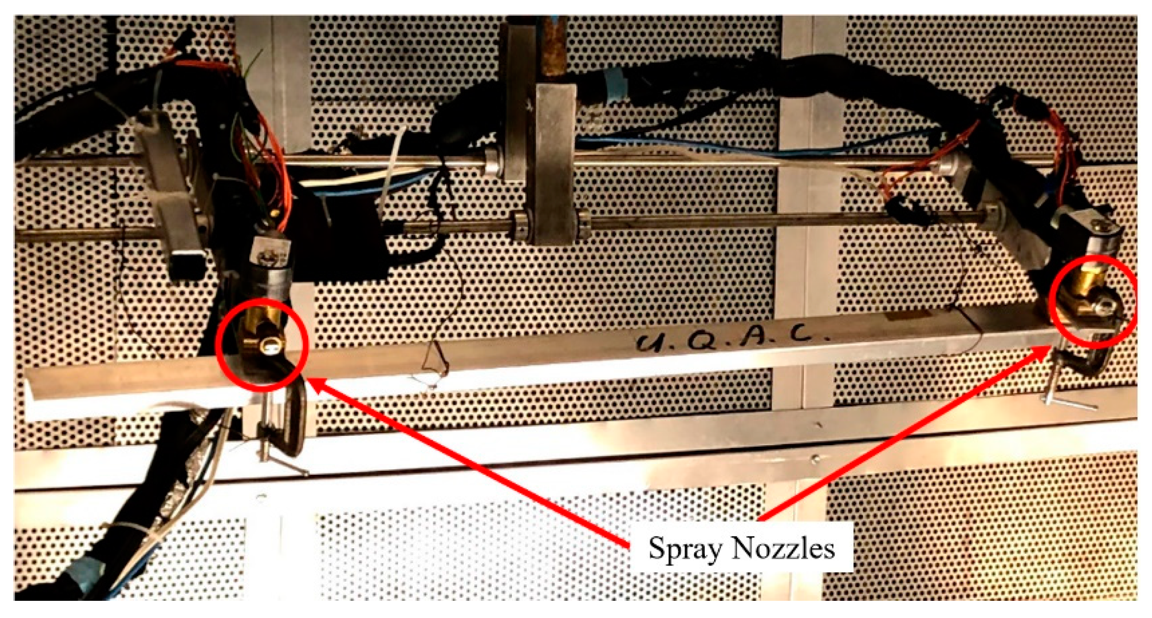
2.2. Icing Nozzle Array

Two icing nozzles were located on the chamber ceiling to generate the icing cloud. A photograph of the spray rig in the ceiling with the two installed nozzles is shown in Figure 2. The nozzles were located at the edges of the array and directly above the center of the rotor shaft to distribute the spray evenly in the chamber. Hydraulic sprinklers produced gravity-fed icing with pressurized nozzle sprayers. Different nozzle heads can be installed to generate different droplet sizes, and heating elements were installed in the system to prevent nozzles from freezing between testing. The droplet speed corresponds to their freefall values in the vertical airflow (see Section 2.6). Distilled water maintained in a refrigerator was used to produce the precipitation. Equal air pressure and water pressure were delivered to each nozzle. Measuring the water and air pressures at the input of the water and airlines to the nozzles ensures precise readings of the pressure differential controlling the droplet size.

2.3. MVD Measurement

To measure the Median Volumetric Diameter (MVD), a thin layer of silicone oil was applied on the surface of a glass slide, as shown in Figure 3. This method, described and recommended in AIR4906 [33], used a glass slide coated with silicone oil, which is passed through the spray range of the nozzles, to collect a certain number of droplets. Due to the incompatibility between oil and water, the droplets were wrapped in silicone oil and kept their original shapes for a short time. The droplets on the glass slide were observed and photographed under a camera; the observation results are shown in Figure 3.

The MVD can be obtained by statistical calculation of droplet diameters. This technique is a commonly used and accepted method in the industry [33]. To obtain different MVD in the cold chamber, different nozzle heads are installed on the nozzle array. In this study, two models are used, a first one to obtain a smaller droplet size representing freezing drizzle precipitation and a second one to obtain significantly larger droplets representative of freezing rain precipitation. This method has been validated using a cloud imaging probe from Droplet Measurement Technologies.

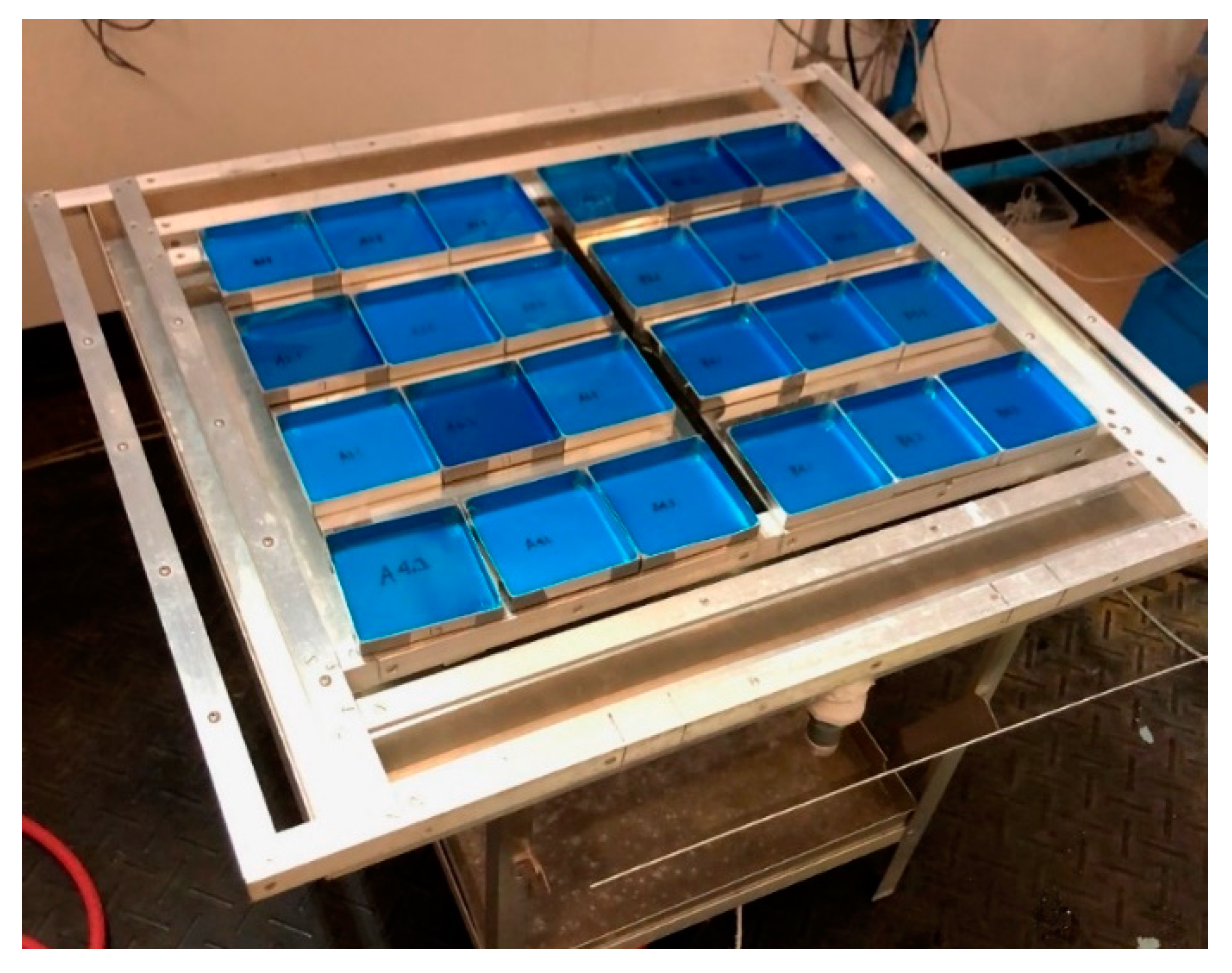
2.4. Precipitation Rate

The Precipitation Rate λ, or Icing Intensity, is a commonly used measure of in-ground and low-altitude icing. This measure represents the mass of water, or frozen precipitation, that falls over an area per unit of time. To measure the precipitation rate in the chamber, a catch pan technique was used, as required in aircraft ground icing standards [34,35] and used in other studies [36]. After choosing and installing the desired spray head, 24 catch pans were placed in the center of the chamber at 2 m, as seen in Figure 4. As shown in the figure, the catch pans (blue interior) were placed on a table at the center of the test section and directly under the icing nozzle array. Each catch pan was individually weighed empty, and its weight was recorded. The spray was activated for a period of up to 30 min and the pans were again weighed together with the collected amount of water. The difference between the two sets of recorded weights is the weight of the collected water, which is then used to calculate λ with the Equation (1). M_W is the mass of collected water in g and t_prec is the precipitation collection time in min. This measurement setup respects the requirements of the industry standards [34,35]. In addition, multiple measurements were repeated throughout the test campaign to ensure the stability of the precipitation rate.

$$\lambda =\frac{M_W}{t_{prec}}\times 60$$

(1)

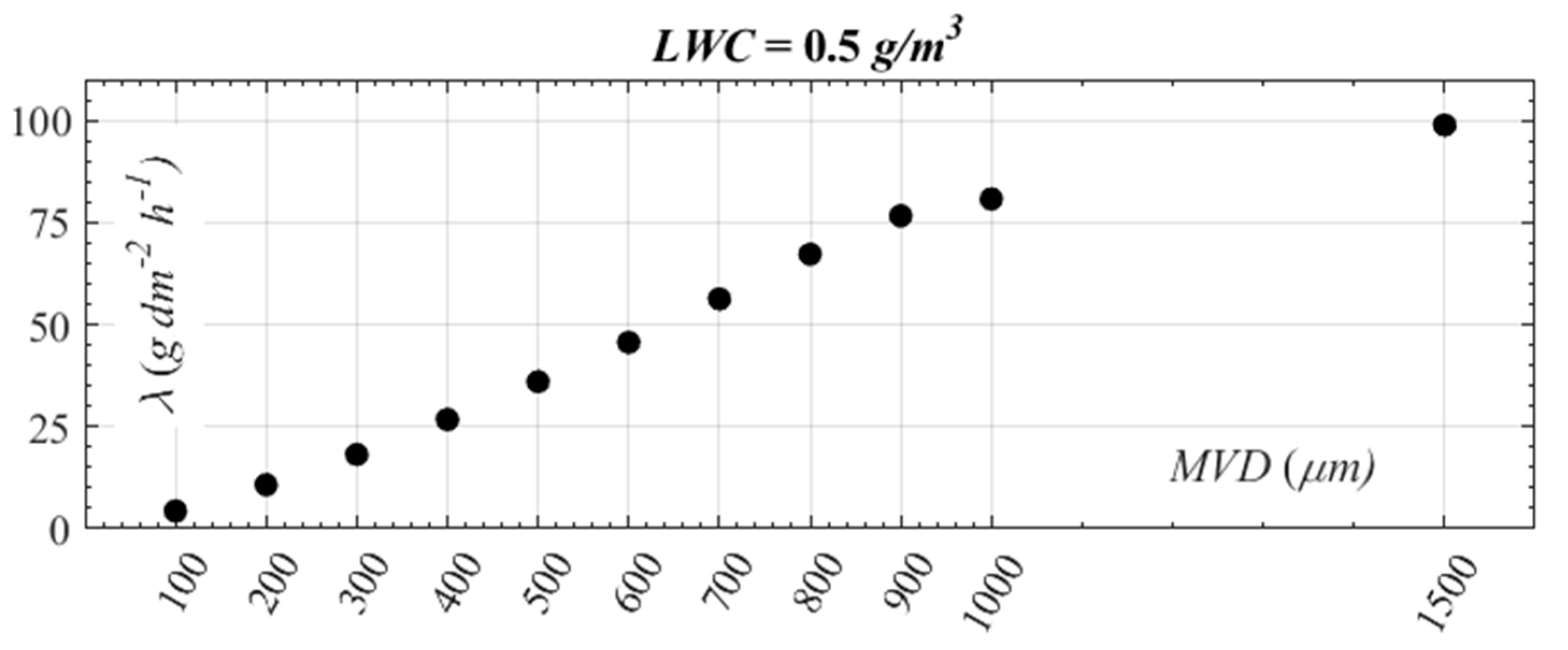
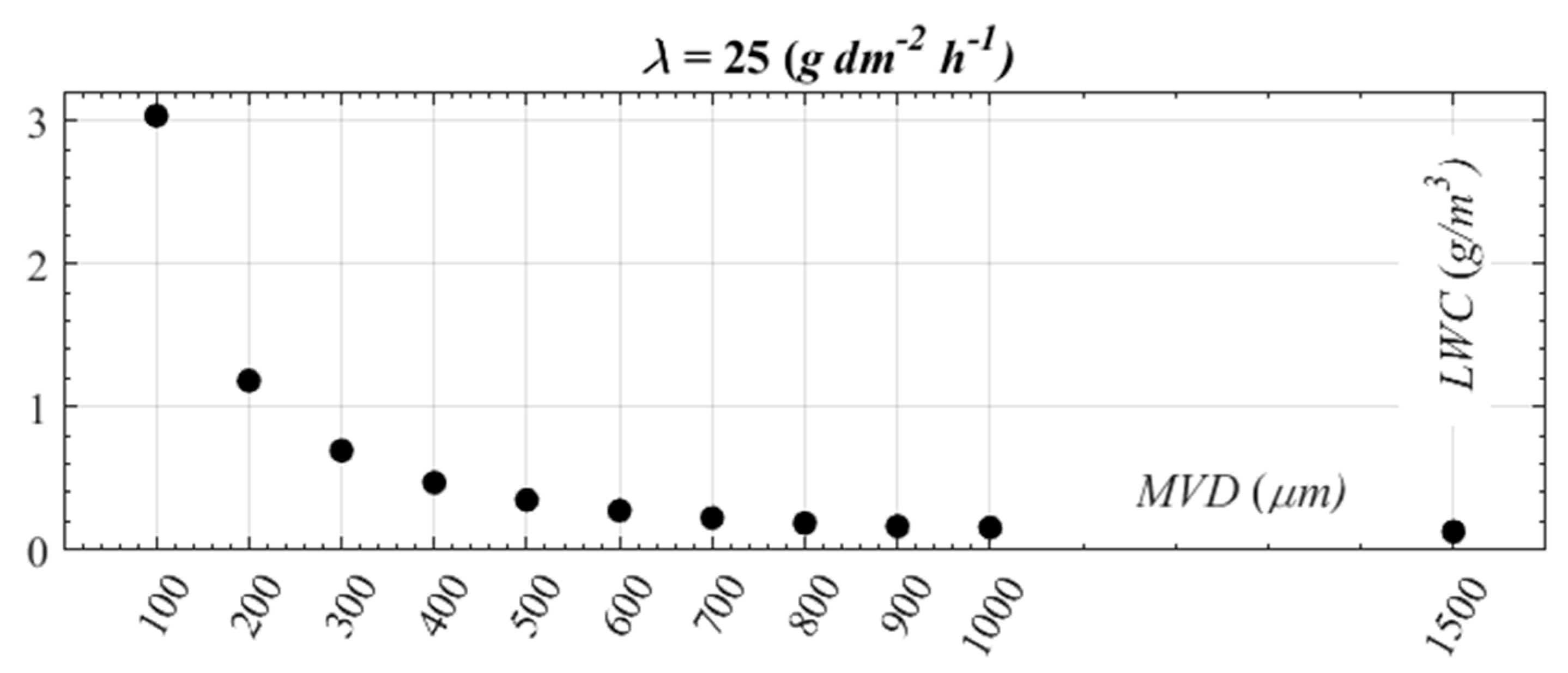
2.5. LWC Estimation and Droplet Velocities

The Liquid Water Content (LWC) is a measure of the mass of water contained in a volume of air. This value is commonly used for in-flight icing but also for ground and low altitude icing. LWC sensors, like the King probe or rotating cylinder methods [37], can be readily used to measure the LWC in an icing cloud. However, those sensors either require a certain flow velocity (usually 10–15 m/s and higher) to function properly or must use the flow velocity in the calculation to determine the LWC value from their measurements. In-ground icing and low altitude hover mode, unlike in wind tunnel, no airflow is generated during the calibration of the icing conditions, making those sensors unreliable since the airflow value is close to 0. This makes the use of the LWC as a parameter impractical for this kind of testing and very difficult to perform a direct comparison between λ and LWC. Another method [27] required measurement of ice accretion on the rotor in order to calculate the LWC, but it is dependent on blade shape, which is not suitable for an easy universal LWC measurement, as well as the particular blade profile used in this study. LWC measurement is a common and recurrent problem in the domain, especially since most standards use LWC for their requirements for in-flight and low altitude icing like the FAA/AR-09/45 [38] and AC29-2C [39], while most standards use λ [34,40] for ground icing.

A new methodology is developed to settle this problem and calculate LWC in the cold chamber for hovering rotor tests and perform a direct comparison to λ to match all the different industry standards. The new methodology calculates the terminal velocity of the water droplets based on the freefall equations and mass balance of the droplet. The velocity is then used together with λ to determine the LWC in the chamber.

In this work, the water droplets are assumed to have the shape of a sphere while dropping from the nozzles downwards. The data for the drag coefficient C_D of a sphere are obtained as a function of Re from the literature. The Re for a sphere is calculated by Equation (2). For simplicity, the C_D is calculated using a linear interpolation presented at Equation (3), of the well-established drag coefficient and Reynold’s number relationship between 0 ≤ Re ≤ 1000 [41]. It is acceptable to use that approximation in that first section of the relationship, as demonstrated by the correlation coefficient of R² = 0.9851. Past this region, for 1000 ≤ Re ≤ 100,000, the C_D is constant at 0.3. During this test campaign, it is not expected to test with water droplets with an MVD higher than 800 μm. At this size, the sphere Re is approximately 200, which is well below the higher boundary of the Re correlation. V_T is the terminal velocity of the water droplet, and 𝜗_air = 0.00001328 m²/s is the kinematic viscosity of air.

$$Re=\frac{V_{T}D}{{\vartheta }_{air}},$$

(2)

$$C_D=28.651\ast R{e}^{-0.722},$$

(3)

A force balance on the freefalling water droplet results in the gravitational and drag force (D) to be present on the droplet, as expressed in Equation (4). M_Droplet is the mass of the droplet in kg, and a is the acceleration in m²/s. The force from the droplet mass can be expressed by Equation (5), relating the water density (𝜌_w = 997 kg/m³) to the sphere volume (V_Droplet) and the gravitational acceleration (g = 9.81 m/s²). r is the radius of the water droplet in meters.

$$F={\left(M-D\right)}_{Droplet}=M_{Droplet}\ast a,$$

(4)

$$M_{Droplet}={\rho }_w\ast V_{Droplet}\ast g={\rho }_w\ast \frac{3}{4}\pi r^3\ast g,$$

(5)

The drag force, which is linked to the sphere drag coefficient C_D, is obtained from Equation (6). C_D can be obtained from Equation (3) once the Re for the droplet is obtained. The density of air used is 𝜌_air = 1.2922 kg/m³, while the density of air will be different slightly different at lower temperatures, up to 1.367 at −15 °C; calculations indicate that the final terminal velocity calculations would only be impacted by less than 2.2%.

$$D_{Droplet}=\frac{1}{2}{\rho }_{air}\ast V_T^2\ast A\ast C_D=\frac{1}{2}{\rho }_{air}\ast V_T^2\ast \pi r^2\ast C_D,$$

(6)

Once all the terms are rearranged and considering zero acceleration of the droplet, the terminal velocity of the droplet is expressed with Equation (7). V_T can then be used together with the precipitation λ (g dm⁻² h⁻¹) to calculate the liquid water content LWC (g/m³), as described in Equation (8). The conversions of λ are outlined in Equation (9).

$$V_T=\sqrt{\frac{8}{3}r\ast \left(\frac{{\rho }_w}{{\rho }_{air}}\right)\ast \left(\frac{g}{C_D}\right)},$$

(7)

$$LWC\left(\frac{\mathrm{g}}{{\mathrm{m}}^3}\right)=\frac{\mathsf{\lambda }\left({\mathrm{g}\ast \mathrm{m}}^{-2}{\ast \mathrm{s}}^{-1}\right)}{V_T\left({\mathrm{m}\ast \mathrm{s}}^{-1}\right)},$$

(8)

$$\mathsf{\lambda }\left({\mathrm{g}\ast \mathrm{m}}^{-2}{\ast \mathrm{s}}^{-1}\right)\ast 60\ast 60\ast {10}^{-1}\ast {10}^{-1}=\mathsf{\lambda }\left({\mathrm{g}\ast \mathrm{dm}}^{-2}\ast {\mathrm{h}}^{-1}\right),$$

(9)

To calculate the distance required for a droplet to reach its V_T, a time-dependent approach is taken. For every time step Δt, the droplet velocity V_i+1 is calculated by using Equation (10) where V_i is the droplet velocity at the previous timestep and a_i is the droplet acceleration. a_i is calculated using Equation (11) by applying the force balance shown in Equation (4). The distance traveled between the two timesteps Δh is then calculated using Equation (12). The procedure is looped until the droplet acceleration is zero, where the terminal velocity is reached.

$$V_{i+1}=V_i+a_i\ast \Delta t,$$

(10)

$$a_i=\frac{M_W\ast g-D_{Droplet}}{M_W},$$

(11)

$$\Delta h=\left(V_{i+1}+V_i\right)\ast 0.5\ast \Delta t,$$

(12)

The distance traveled by a droplet before reaching its V_T, calculated as a function of droplet size, is presented in Figure 5. The figure shows droplet sizes between 100 μm and 1500 μm. For small droplets, V_T is reached for heights as low as 0.05 m, whereas bigger droplets require a higher distance to reach their V_T. For a droplet size of 1500 μm, a height of almost 8 m is required.

In this research, the droplets used have an MVD of either 120 μm or 800 μm. According to Figure 5, the droplets at 120 μm need 0.04 m to reach their V_T whereas those at 800 μm need at least 4 m. Provided that the nozzles are at a height of 9 m, and that the rotor is tested between 2 m and 4 m off the ground, then the distance between the rotor and nozzles during tests will be between 5 m and 7 m. This range then satisfies the height requirement for the used droplets and therefore agrees with the methodology of LWC calculation.

Based on the above, and with the proper height requirement to reach the V_T for each droplet size, the λ needed to produce an LWC = 0.5 g/m³ can now be calculated. A LWC of 0.5 g/m³ is typical for freezing rain and freezing drizzle outside clouds, according to FAA/AR-09/45 [38]. Figure 6 shows the variation of λ needed to produce a LWC = 0.5 g/m³ for the variety of droplet sizes. As the figure shows, a higher λ is needed when the droplet size increases. A maximum of 100 g dm⁻² h⁻¹ was estimated for a droplet size of 1500 μm. For the MVD selected for testing, the λ for a LWC = 0.5 g/m³ is around 5 g dm⁻² h⁻¹ for 120 µm and around 73 g dm⁻² h⁻¹ for 800 µm.

In a similar analogy to the preceding section, the LWC produced based on a λ of 25 g dm⁻² h⁻¹ is investigated which is typical for ground icing. Figure 7 shows the variation of the LWC versus the droplet size that is obtained for a λ of 25 g dm⁻² h⁻¹. For the fixed λ, the LWC produced decreases with increasing droplet size, varying between 3 g/m³ at 100 μm down to almost 0.1 g/m³ for a droplet size of 1500 μm. For the MVD selected, this corresponds to a LWC of 2.53 g/m³ for droplets of 120 µm and a LWC of 0.19 g/m³ for droplets of 800 µm.

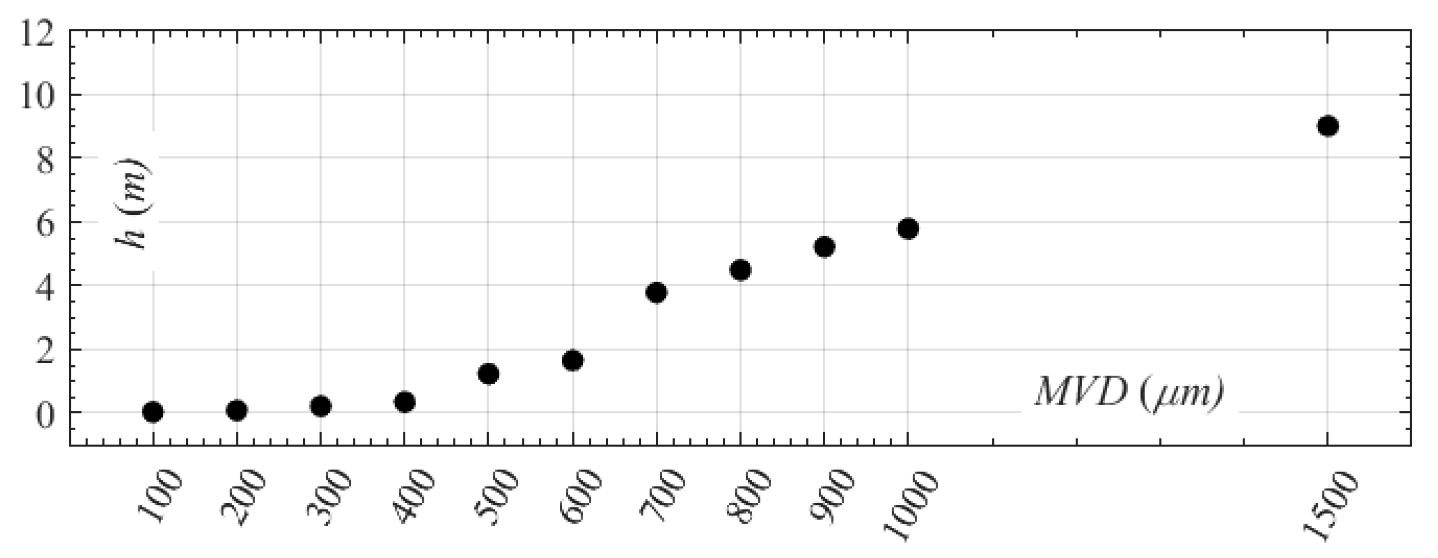
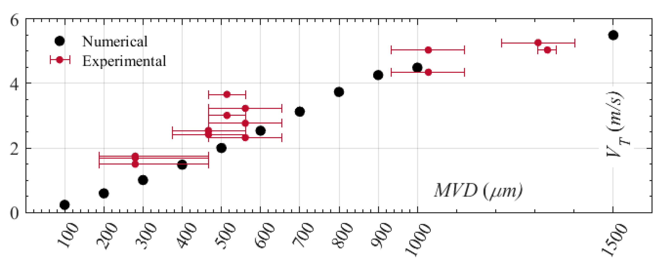
2.6. Tracking the Droplets’ Terminal Velocity

An experiment was conducted to validate the water droplets terminal velocity after falling from the chamber’s ceiling, making sure the calculations from the previous section were correct and to confirm that the droplets had reached terminal velocity at rotor height. For the experiment, the chamber was darkened, and a light source was placed behind the falling stream of water. A camera was used to take photos of the falling water droplets at a rate of 200 photos per second (a picture every 5 ms). Using a ruler as an established scale, the distance traveled by a single droplet between two photos was then measured using digitizing software. A cover with a single slit is installed on top of the camera to obtain a single slice of droplets falling at a single and known distance from the camera. Knowing the time difference between the photos from the rate of the camera, the velocity of the droplet could be calculated. This was done for many droplets, of both similar and different sizes, to confirm the consistency between the velocities of the different droplets and validate the calculation for the whole range of droplet size generated. This simple setup was developed to strengthen confidence in the theoretical calculations done at the previous section, using simple and widely accepted theory, and for this reason the precision of the method was deemed sufficient.

2.7. Ice Shape Documentation & Measurements

An apparatus and a methodology were developed to document the ice shapes and its measurements in this experimental campaign. A database of photographic images, thickness measurements and 3D scans was created. For the 2D photographs, a custom-built rig was fabricated to hold a high-resolution camera in place, at a focal distance from the blade. The rig has three positions for the camera that enabled taking photos of the blade and ice from the front, side and top of the blade in a consistent manner between tests, similar as those presented in [5,36].

As for the ice thickness measurements, one blade was selected as a control blade where straight lines were drawn using a water-resistant ink at 9 different radial locations between the root and tip of the blade, as shown in Figure 8. A digital caliper was used to measure the chord at those locations without ice and then used again after each test to measure the new chord with the accumulated ice. A subtraction of the former from the latter will result in the chordwise ice thickness at the leading edge found at the marked radial locations. Those thicknesses will serve as a simple indication of the severity of the ice accumulation along and in addition to the pictures and scan gathered.

Finally, multiple 3D scans of the ice accumulation were also gathered. Figure 9a shows a sample scan of the clean rotor blade, prior to any icing exposure. The result of a scan with accumulated ice is shown in Figure 9b. Three different models of 3D scanners from the company Creaform were used to scan the blade with its accumulated ice: the GoSCAN 50, using white light technology, the HandySCAN 307/700, using a red laser, and the HandySCAN Black, using a blue laser. The white and opaque rime ice was easier to scan due to its better reflection of the light than the clear glaze ice. To help with clear glaze ice, very fine clay powder was brushed on the ice layer. Not all types of 3D scanners were able to provide a satisfactory scan of glaze ice, and the red-light model was deemed the most suitable one for this testing. The VXelements software was used to obtain the 3d images.

2.8. Icing Conditions

To select the icing conditions for testing, two main standards are used: the FAA/AR-09/45 [38] and the SAE standards ARP 5485 [34] and AS5901 [40]. Those documents determine conditions for ground and low altitude icing. The two types of precipitation selected are freezing drizzle and freezing rain. In [34,40], the droplet size for freezing drizzle is 300 µm and for the freezing rain is 1000 µm, while in FAA/AR-09/45, it is 120 µm and 800 µm respectively. The two droplet sizes selected are 120 μm and 800 μm, corresponding to nozzle heads readily available at the laboratory. The SAE documents specify the precipitation rate for the icing precipitation with the more severe condition set at 25 g dm⁻² h⁻¹. In the FAA document, however, the icing precipitation requirements are expressed in terms of LWC, with values of 0.4 to 0.5 g/m³ for both freezing drizzle and freezing rain. For simplicity, a single value of 0.5 g/m³ is considered in this test campaign. The technique and calculations developed and detailed in the previous section are used to compare and convert LWC to λ. In addition to those two requirements, an additional requirement of 0.25 in of water per hour is also defined by the industrial partner itself. The comprehensive grid of icing conditions selected for the whole test campaign and the rationale for each of those conditions is presented in

Table 1. Details of icing parameters used for tests along with their rationale.

λ (g dm−2 h−1)	MVD (μm)	LWC (g/m3)	Rational
5	120	0.47	0.5 g/m3 (FAA/AR-09/45)
25	120	2.35	Typical Ground Icing + Light Rain (2 L/h/m2)
25	800	0.19	Typical Ground Icing + Light Rain (2 L/h/m2)
67	120	6.31	0.25 in. Water/hr for APT70 Requirement + Moderate Rain (6 L/h/m2)
67	800	0.50	0.25 in. Water/hr for APT70 Requirement + 0.5 g/m3 (FAA/AR-09/45) + Moderate Rain (6 L/h/m2)
80	120	7.53	Typical Ground Icing + Moderate Rain (8 L/h/m2)
80	800	0.59	Typical Ground Icing + Moderate Rain (8 L/h/m2)

. For the preliminary testing performed in this paper, only the conditions in bold were used.

Aside from the water spray parameters, the air temperature in the cold chamber plays a crucial role in the type of accumulated ice. To make sure rotor icing is studied for the glaze, rime, and mixed ice conditions during the experimental campaign, three air temperatures are used. These are T_∝ = −5 °C, −12 °C, and −15 °C. The highest T_∝ used was −5°C since ice accumulation was poor or not possible when temperatures of −2 °C or 0 °C were used. For the preliminary testing of this study, only results at T_∝ = −5 °C and −15 °C are presented.

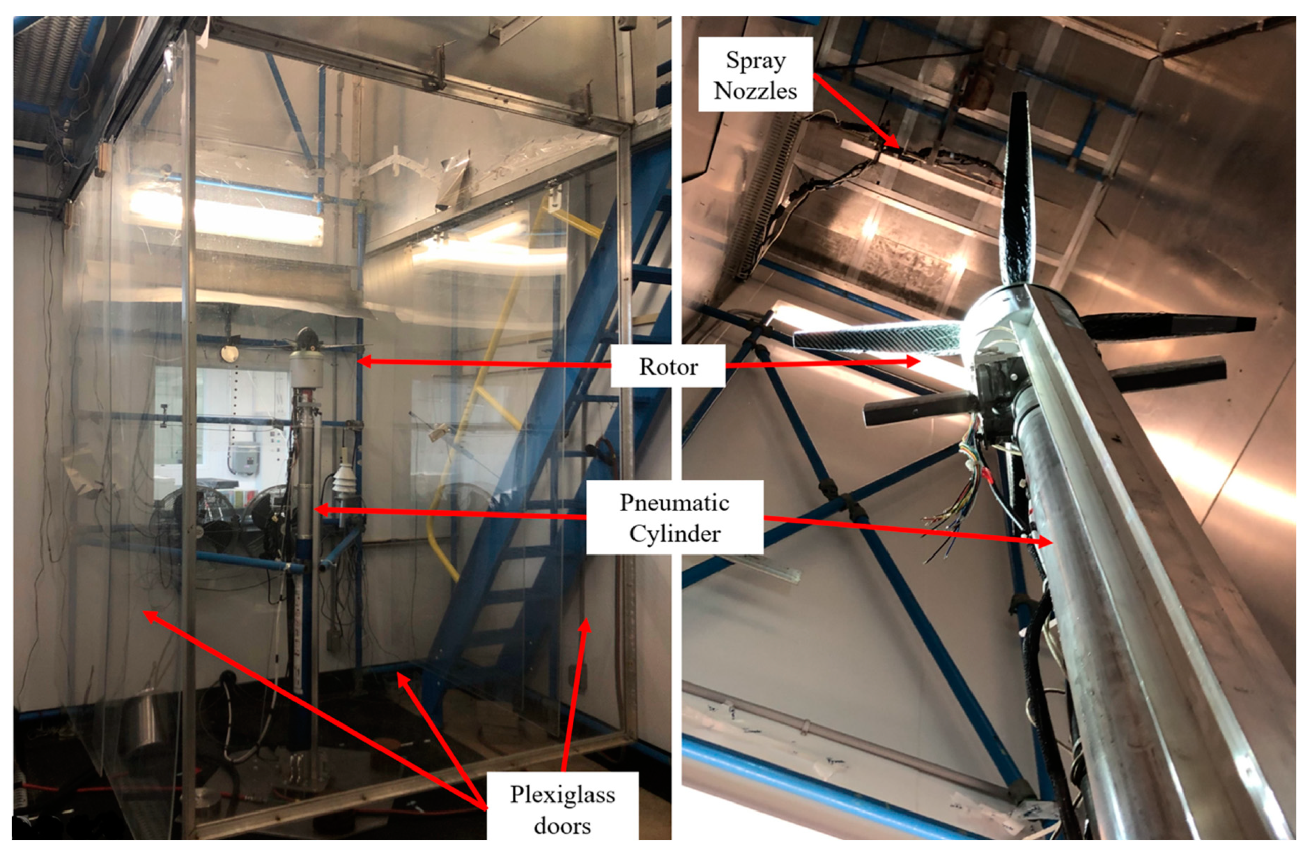
3. Materials and Methods: Drone Rotor Setup

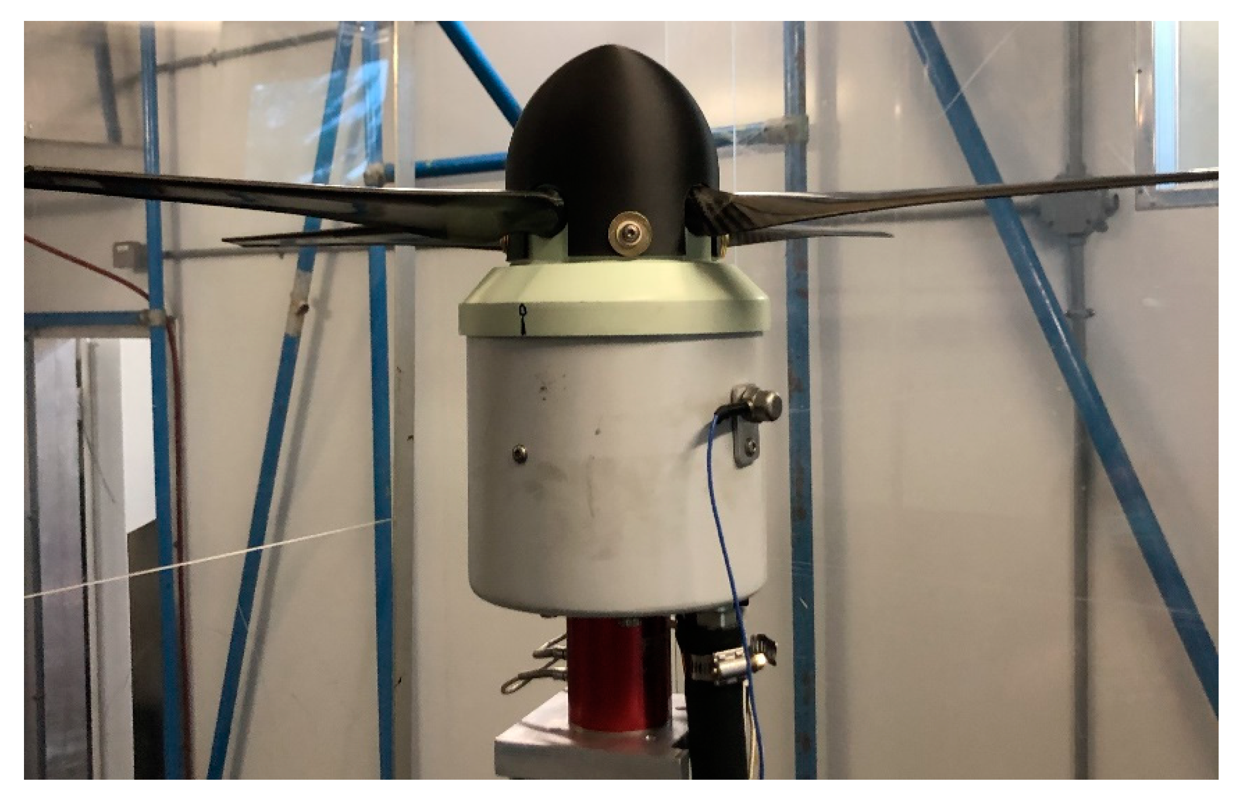
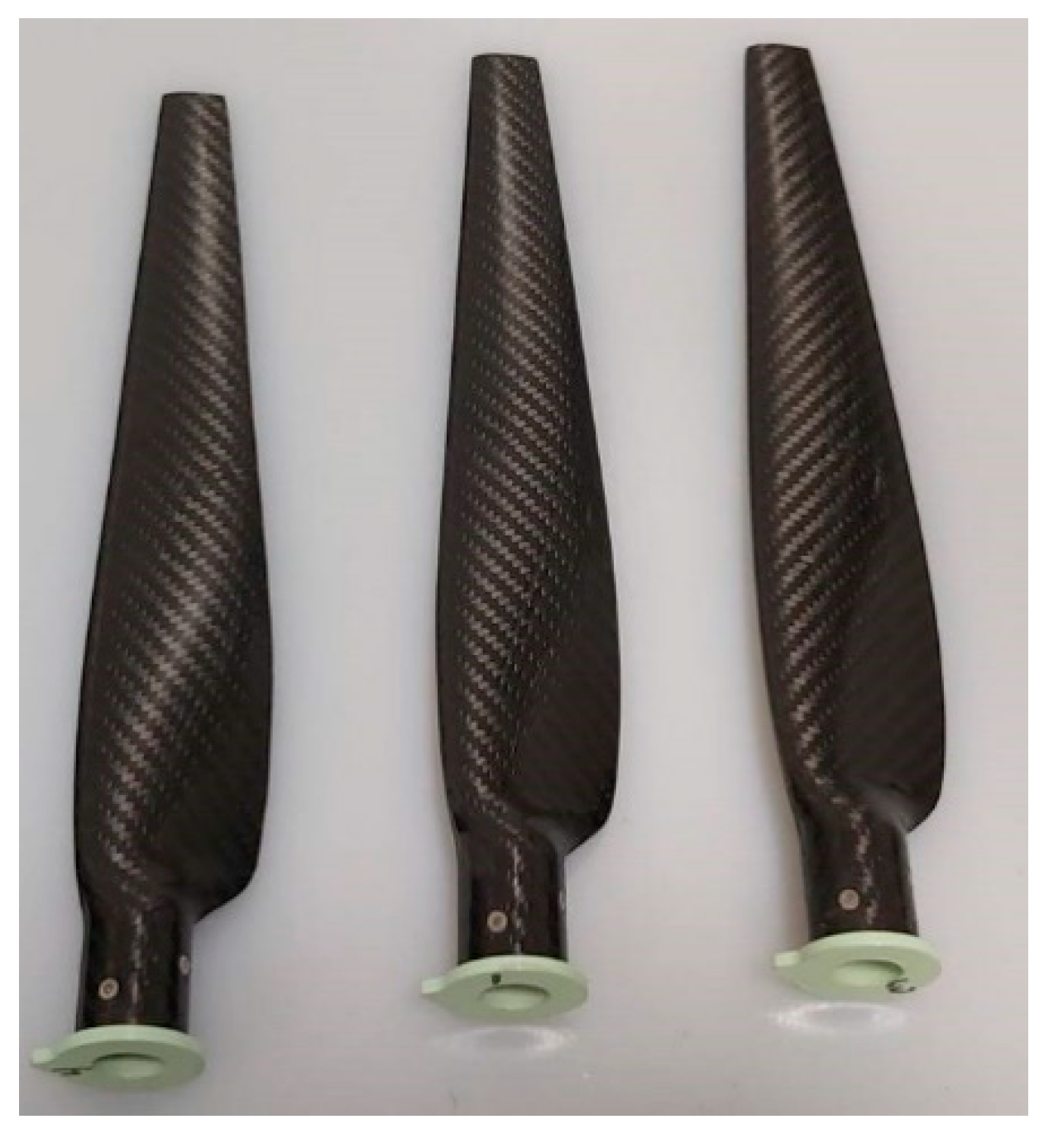
3.1. Drone Rotor Assembly

In the center of the chamber, a 12-kW Hacker Q150-45-4 motor is used to power the drone’s rotor. The motor and hub system is installed in the center of the chamber’s test section on a pneumatic cylinder, as shown in Figure 10, to test different rotor heights. Compressed air is supplied to the motor via an external feeder to increase operation time before overheating the motor. To measure thrust, torque and mechanical power consumption of the rotor, a two-axis Futek MBA-FSH04262 load cell was added between the motor and the holding post. Data acquisition, as well as control of the rotor system, is performed using a custom Labview interface. This measurement and control system has been extensively tested and used by the industrial partner for other aerodynamical studies.

The rotor studied in this experiment is the slightly modified 81% scaled version of the Bell APT70 drone rotor. The modifications are related to the root attachment, which is circular on the subscale rather than rectangular. For both rotors, the blade roots are mostly covered by a spinner cone which should not make a significant difference. It has four blades (presented in Figure 11) with a diameter of 0.66 m and a NACA 4412 aerodynamic profile. Each blade is formed of two carbon fiber parts that are glued together to form one hollow blade 25.4 cm long. The blades are twisted and have a variable chord from root to tip. Equations (13) and (14) are used to describe the curve fitting result based on the non-dimensional radial location r for the twist φ (°) and chord c (m), respectively. The configuration can reach 6000 RPM, reproducing the full-scale drone maximum tip speeds.

$$\phi =-65.187r^3+169.58r^2-161.36r+68.5,$$

(13)

$$c=\left(-10.632r^4+30.997r^3-33.185r^2+13.566r+0.0397\right)\ast \frac{2.54}{100},$$

(14)

3.2. Rotor Test Parameters

In order to better understand the impact of ice accretion on rotor performance in hover conditions for a drone like the Bell APT70, icing tests are to be conducted at different speeds, air temperatures, droplet sizes, and precipitation rates are required. Three levels of RPM are targeted for a comprehensive investigation: low, medium and high. Since the rotor studied in this experiment is a scaled-down version, it is important to set similarity parameters with the full-scale APT70 rotor. Similar tip speeds are expected to produce similar aerodynamic performances and flow behavior. Similar centrifugal forces are expected to produce similar ice accretion and ice shedding. It is not possible to match both parameters at the same time, so for each level of RPM investigated for the full-scale rotor, two RPM values are obtained for the scaled-down model, one to match the tip-speed and one to match the centrifugal force of each level, resulting in a total of six RPM values for experimental testing (

Table 2. Calculated RPM Values for the Scaled-Down Rotor.

Thrust Level	Scaling Rule	RPM
Low	Same centrifugal force	3880
	Same tip-speed	4300
Medium	Same centrifugal force	4440
	Same tip-speed	4950
High	Same centrifugal force	4950
	Same tip-speed	5540

).

4300 RPM is close to 4440 RPM and is then rejected to minimize the number of tests. Only 3880, 4440, 4950 and 5540 are kept. However, during preliminary testing with icing spray, it was remarked that the electrical power consumption for tests at Ω = 4950 RPM reached around 11 kW. Therefore, to avoid exceeding the rated motor power of 12 kW, rotor speeds for icing tests were limited to 4950 RPM.

Table 3. List of Tested Rotor Speeds and Rotor Heights.

Height (m)	Ω; Icing Tests (RPM)
2	3880
	4400
4	4950
	4950

lists the different Ω and rotor heights h used for the icing tests at the different icing conditions selected (II.H).

3.3. Testing Procedure

Icing tests were conducted in the cold chamber following a specific protocol that ensures the safety of the personnel, maintains the healthy operation of equipment and provides reliable and consistent results. The procedure is outlined step-by-step as follows.

• The motor cooling air is first turned on, followed by the power supply for the motor. The rotor spin safety switch is then deactivated, and the test begins. The test is initiated in the software and data acquisition starts recording.
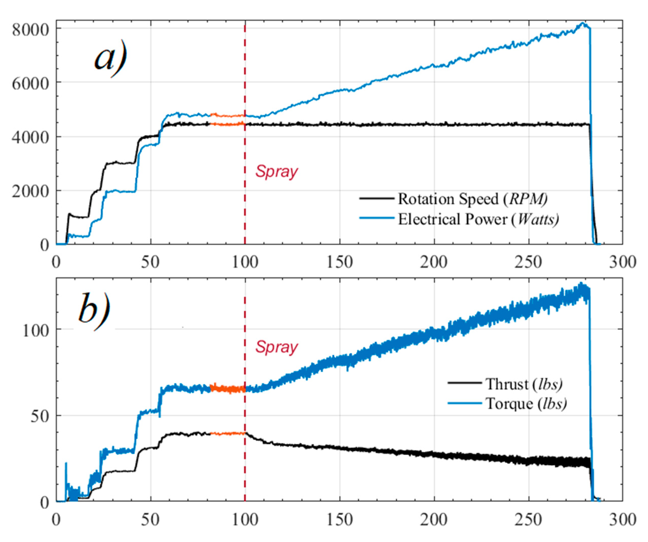
• The rotor speed is incrementally increased from 0 to the desired steady-state speed. After a short stabilization period at the target rotation speed, the water spray is activated, and ice accumulation begins where the torque and electrical power consumed continuously increase and thrust decreases. The vibration levels, motor temperature and electrical power consumed are closely monitored throughout the spray time.
• The test is stopped whenever one of those conditions happens; (listed in the order of actual occurrence during tests): 1- ice sheds from the blade, causing severe vibrations (>2 Inches Per Second (ips)) OR when the vibration levels reach 2 ips even without ice shedding; 2- the electrical power consumed approaches the rated power of the motor (12 kw); 3- the test duration exceeds 20 min and; 4- the motor temperature reaches 100 °C.
• After the test is concluded, the motor alimentation is switched off and the safety switch of the rotor is activated. A visual inspection of the equipment is first done to check for any damage.
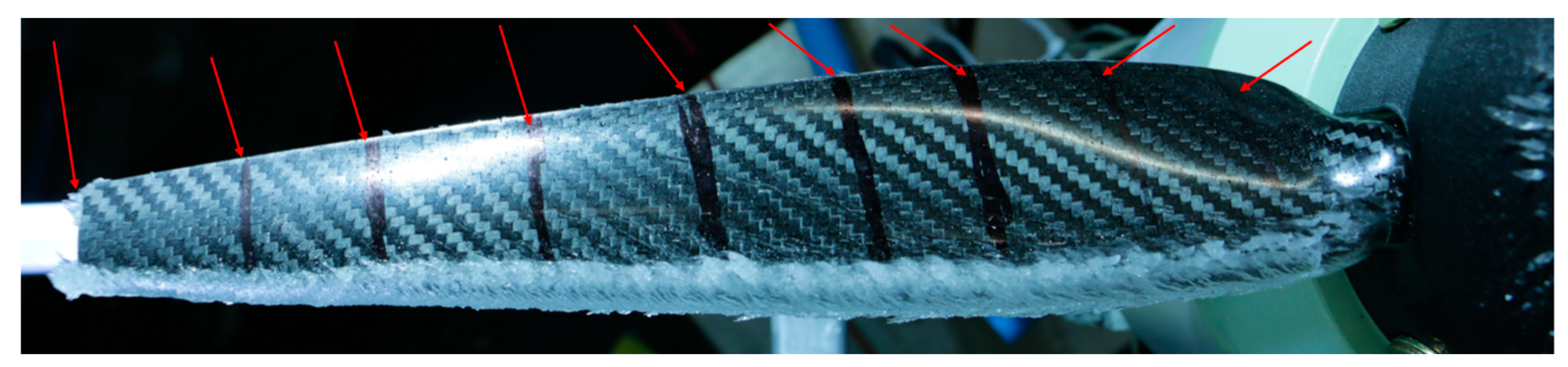
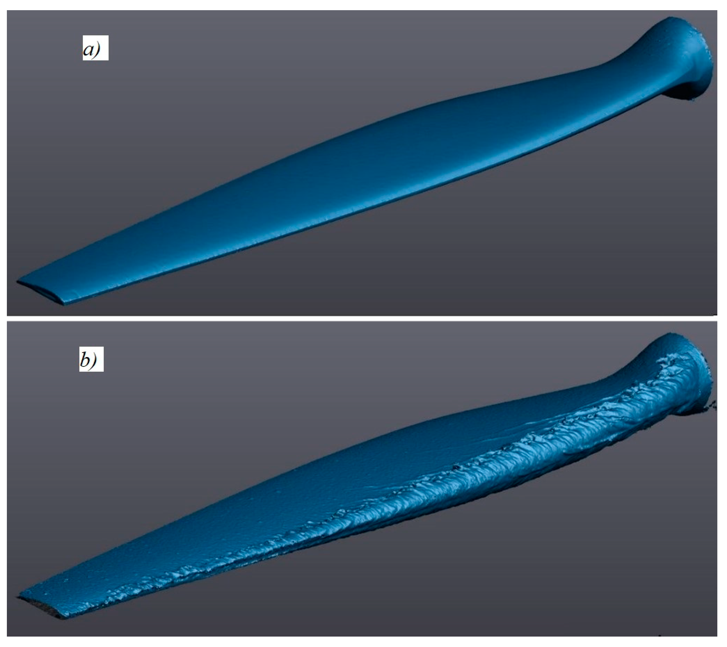
• The photography platform is then installed on the rotor pole, and photos of the ice shape are taken from the front, side and upper directions. A scan is performed of the ice accumulation with the 3D scanner and a digital caliper is then used to measure the ice thickness at 9 different and pre-marked blade locations.
• Finally, the ice is then melted off the rotor using a heat gun and cleaned using industrial grade paper towel to prepare it for the next test.

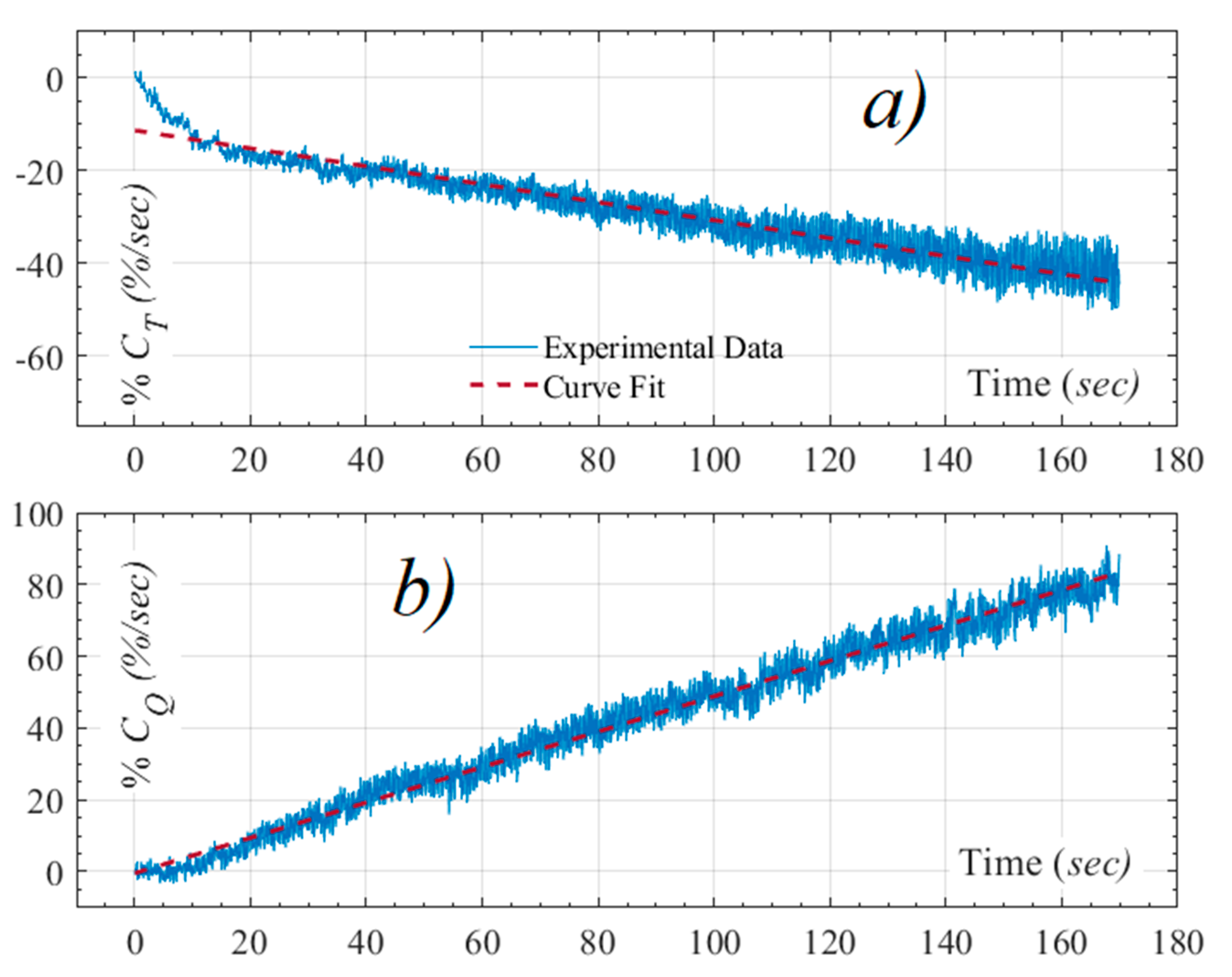
3.4. Post-Processing and Non-Dimensional Coefficients

To analyze the data and determine the severity of each test, non-dimensional coefficients are used for test comparison. The non-dimensional thrust coefficient C_T as well as the torque coefficient C_Q for each test are calculated as shown in Equation (15), where 𝜌 is the density of air (kg/m³), Ω is the rotor speed (rev/s) and d is the rotor diameter (m).

$$C_T=\frac{T}{\rho {\mathsf{\Omega }}^2{d}^4}, C_Q=\frac{Q}{\rho {\mathsf{\Omega }}^2{d}^5},$$

(15)

For each test, average values for each of the recorded parameters during the stabilization period, prior to water initiation, must be established. Figure 12 shows an example of an icing test where the stabilization period is highlighted in orange for all the curves of rotor speed and electrical power (Figure 12a), as well as for the torque and thrust (Figure 12b). The period begins once the rotor reaches the target speed and ends at the beginning of the water spray, which is directly followed by an increase of torque and decrease of thrust.

To observe the effect of ice accretion on rotor performance, the measurements taken during icing are compared to their calculated average values prior to water spray initiation. This is how Figure 13 is obtained, which shows the percentage decline of the measured C_T with time (Figure 13a) as well as the parallel percentage increase of C_Q (Figure 13b), based on their respective average values without ice.

Testing showed that for the absolute majority of cases, the variations shown in Figure 13 are linear or could be curve fitted by a linear variation as shown by the red dashed lines of the figure. Therefore, the severity of a test is then directly related to the C_T slope (referred to as $C_T^{\ast }$ (%/s)) as well as the C_Q slope ($C_Q^{\ast }$ (%/s)). In other words, a test is considered more severe if $C_T^{\ast }$ is lower and $C_Q^{\ast }$ is higher. It should be noted that the C_T slope during icing is always negative, while the C_Q slope is always positive.

It is also interesting to determine the required increase of mechanical power (P⁺) to maintain the same initial thrust without ice in order to use only one output parameter to sort tests by severity. This logic requires the calculation of the required increase of rotor speed (Ω⁺ (%/s)) using Equation (16). The increase of torque required to maintain initial thrust ($C_Q^{+}$ (%/s)) is then calculated using Equation (17), and P⁺ is finally obtained using Equation (18).

$${\Omega }^{+}=\frac{1}{\sqrt{1+C_T^{\ast }}},$$

(16)

$$C_Q^{+}=\frac{1}{1+C_T^{\ast }}\ast C_Q^{\ast },$$

(17)

$$P^{+}=\frac{1}{\sqrt{1+C_T^{\ast }}}\ast C_Q^{+},$$

(18)

4. Results

4.1. Validation of LWC Estimation—Droplet Terminal Velocity

Figure 14 shows the theoretical results of V_T calculation obtained for different water droplet sizes, compared to the experimental data measured using the procedure described in Section 2.6. Numerical data indicate that V_T increases with the droplet size. This ranges from as low as 0.25 m/s at 100 μm to as high as almost 5.5 m/s when the droplet size is 1500 μm. Experimental data show good agreement with numerical predictions, especially when the error bars are considered, principally caused by the determination of the droplet diameters. This basic measurement technique allows for the validation of the theoretical calculations, but the improvement to the technique could be made to increase the accuracy of the measure, and thus a better resolution to measure the droplet diameters.

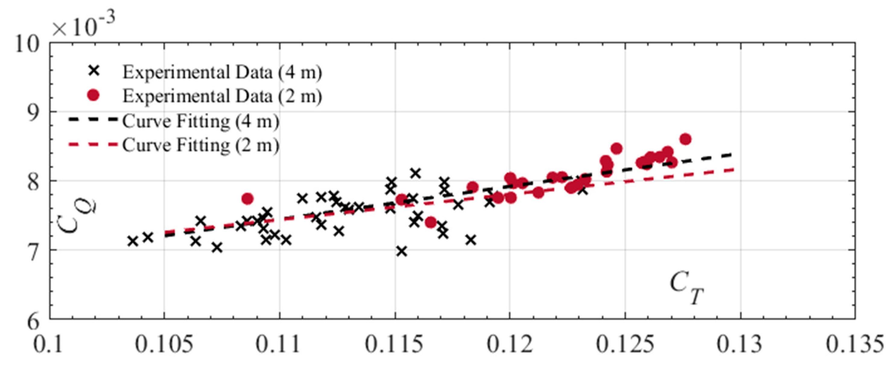
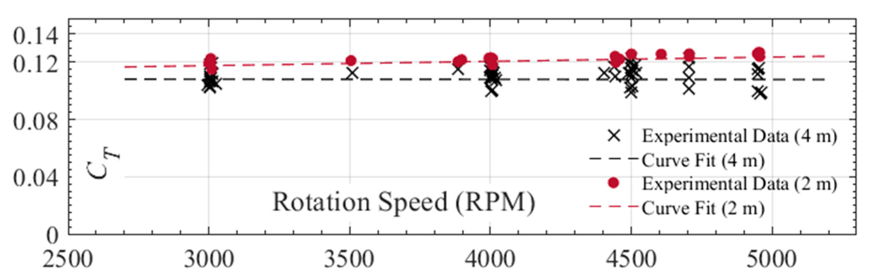
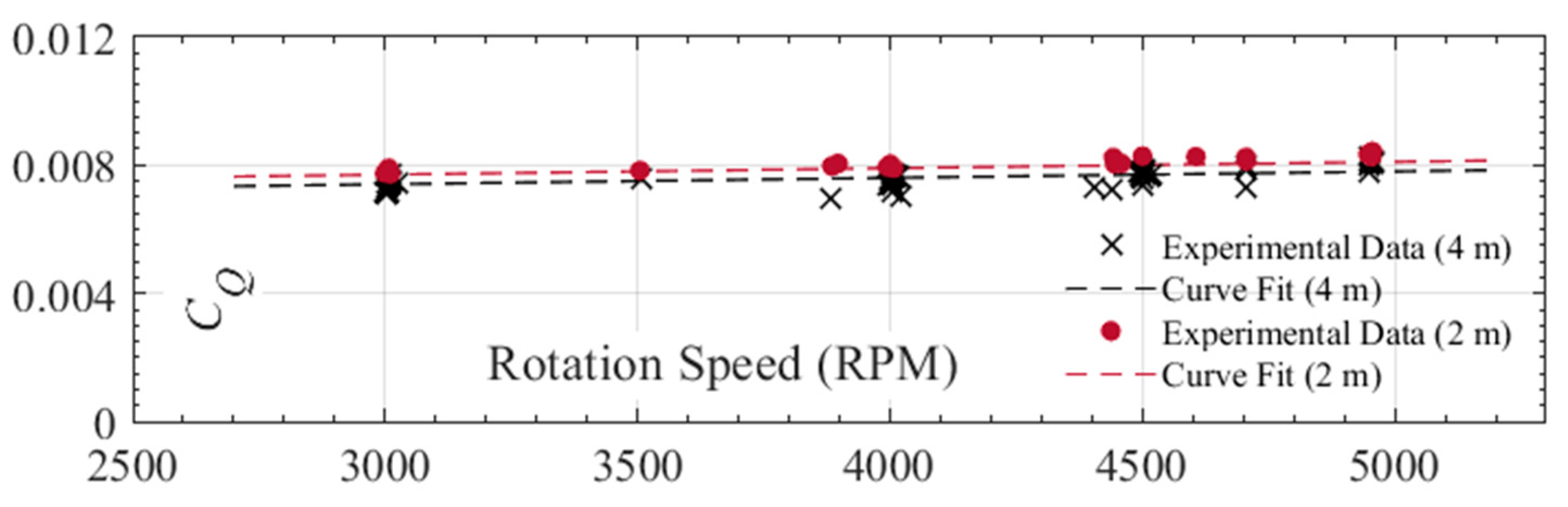
4.2. Assessment of Rotor Height on Ground Effect and Rotor Performance

To determine the minimum distance from the ground to the rotor, preliminary tests at different heights are performed. The test setup, as detailed in Section 2.1, allows testing at heights between h = 2 m and h = 5 m from the ground. For this work, testing is done at h = 2 m and at h = 4 m without blade pitch adjustment. Experimental data for C_T and C_Q were gathered during both dry runs as well as during the initial dry period of icing tests prior to water spray.

Figure 15 shows the variation of C_T versus rotation speed at h = 2 m and h = 4 m. Curve fitting was also applied to each set of data, and the variation obtained is also linear for both. The difference between the curve fitting results of C_T at 2 m, compared to those with the same rotation speed at 4 m, varies between 2.77% at the lowest tested RPM (3000 RPM) and up to 6.53% at the highest (4950 RPM).

Similarly, Figure 16 shows the C_Q variation with Ω for both rotor heights along with their corresponding curve fitting results. The difference between the curve fitting results of C_Q at h = 2 m, compared to those with the same rotation speed at h = 4 m, varies between 4.1% at the lowest tested RPM (3000 RPM) to 3.65% at the highest (4950 RPM).

Finally, the C_T vs. C_Q curve is compared for both sets of measured data at 2 m and 4 m, as shown in Figure 17. A curve fitting scheme is applied to measurement points, and results for both sets at 2 m and 4 m show good agreement. On average, the error between the two curve fittings was around 1.28%. The error is consistent with findings of previous works, where the ground effect is usually absent when h/d > 1 [42], such as in this case. Based on these results, it is possible to assess that there is no significant ground effect at h = 2 m and no significant differences between the rotor performances at h = 2 m and h = 4 m.

4.3. Aerodynamic Parameters at Different Heights—Icing Tests

Table 4. Comparison between calculated aerodynamic parameters for rotor at h = 2 m and h = 4 m; (Tests at Ω = 4950 RPM, θ = 11.7° and λ = 80 g dm⁻² h⁻¹.

MVD (µm)	T∞ (°C)	Height (m)	${\mathit{C}}_{\mathit{T}}^{\mathbf{\ast }}$ (%/s)	${\mathit{C}}_{\mathit{Q}}^{\mathbf{\ast }}$ (%/s)	${\mathit{C}}_{\mathit{Q}}^{\mathbf{+}}$ (%/s)	P+ (%/s)	Icing Time (s)
120	−5	2	−0.124	0.430	0.491	0.524	169
		4	−0.195	0.565	0.703	0.785	114
		Ratio	1.57	1.31	1.43	1.50	0.67
	−15	2	−0.136	0.317	0.367	0.394	162
		4	−0.226	0.400	0.548	0.642	106
		Ratio	1.66	1.27	1.50	1.62	0.65
800	−5	2	−0.036	0.061	0.063	0.065	321
		4	−0.012	0.047	0.048	0.048	761
		Ratio	0.33	0.78	0.76	0.75	2.37
	−15	2	−0.049	0.081	0.085	0.087	326
		4	−0.081	0.121	0.132	0.138	220
		Ratio	1.65	1.49	1.55	1.58	0.67

presents the results of the calculations for the preliminary icing tests done at h = 2 m and h = 4 m. The table compares tests performed with the exact same cold room and spray nozzles configuration, with the only difference being the rotor height. The main reason for this comparison is to study the effect of rotor proximity to the nozzles. The tests in the table were all done at Ω = 4950 RPM, θ = 11.7° and λ = 80 g dm⁻² h⁻¹, with the MVD and T_∞ also specified in the table.

For all the cases tested, except for MVD = 800 µm at T_∞ = −5 °C, the performances of the rotor at h = 4 m degrades between 1.27 to 1.66 faster than at h = 2 m. This is also reflected in the shorter icing time at h = 4 m before testing has to be stopped. The measurements of the icing precipitation intensity (λ) was done at a h = 2 m. To explain this difference, new measurements of the precipitation intensity are repeated at h = 4 m, with the nozzle settings defined during calibration at h = 2 m. Due to the fact that the icing cloud is not fully dispersed in the test section area and is more concentrated, the precipitation intensities obtained at h = 4 m are 1.3 to 1.4 times higher compared to those obtained for the same nozzle settings at h = 2 m for both droplet sizes. The water spray angle and area of coverage are smaller at h = 4 m than at h = 2 m, so a higher λ is obtained, explaining the difference in the results.

Results differ when the larger droplets (MVD = 800 µm) are used at T_∞ = −5 °C. The aerodynamic performances decreased more slowly at h = 4 m than at h = 2 m in opposition to what is obtained at the other test conditions. This can be explained by the fact that some of the larger water droplets of the distribution spectrum are not reaching freezing temperature while falling from the nozzles. The larger droplets are expected to take a longer time during the free fall to reach freezing temperature, and the shorter distance between the rotor and nozzles at h = 4 m seems to lower ice accretion at a warmer temperature like T_∞ = −5 °C. At h = 2 m the hub and blades are 7 m away from the nozzles, while at h = 4 m they are only 5 m away. The droplets are released around 0 to 1°C and cool down during their freefall. With the aerodynamic heating, those very large droplets after a freefall of only 5 m take much longer to freeze on the blade due to their higher temperature when they reach the rotor, and most of them are expulsed from the rotating blades. The expulsion of droplets from the blades could be observed visually during testing. This could also be observed by the lower vibration rates during the test, as well as with the lower amount of ice that was accreted when the test was finalized and longer test durations.

Keeping in mind that the performances of the rotor without ice were similar between h = 4 m and h = 2 m, and since the icing parameters are calibrated at h = 2 m, it is decided that the test campaign will be performed at h = 2 m. On the other hand, the differences brought by the rotor height during icing pose an interesting topic to be elaborated in future studies, especially on the large droplets’ temperature equilibrium.

5. Conclusions

This paper presented the design process and methodology used to develop an innovative experimental test rig to study the effects of icing on the rotor of a Bell APT70 drone in take-off/hover flying mode. The test rig was installed in the 9-m-high AMIL cold chamber whose unique capabilities allowed to study the ground effect and rotor proximity to the icing nozzle array at different rotor heights. Techniques for the measurement of MVD and λ in the chamber are presented, followed by a new methodology to calculate the LWC for a rotor in hover flight, based on the MVD and λ.

A preliminary experimental comparison of aerodynamic parameters between rotor heights at h = 2 m and h = 4 m showed no difference in the results, demonstrating that no ground effect is obtained at h = 2 m, and further icing tests were therefore decided to be carried out at that lower height, with the advantage of experimental convenience and extra distance from the nozzles. When icing tests were carried out at a distance of 7 m from the nozzles to the rotor (h = 2 m) and at 5 m (h = 4 m), the icing accumulation was changed at warm temperatures for the larger droplets. The larger droplets at that warmer temperature did not cool enough, and very few droplets froze on the blades after a freefall of only 5 m (h = 4 m). The larger droplets of the spectrum did not totally reach terminal velocity either. For those reasons, the decision to position the setup at h = 2 m (7 m from the nozzles) was taken.

Following this important study on the development of a unique test right, a comprehensive investigation on the impact of drone rotor icing can now be undertaken. The effects of Pitch Angles θ, Liquid Water Content (LWC), Median Volume Diameter (MVD), air temperatures T_∞, rotor speeds Ω and precipitation rates λ on rotor performance and resulting ice accumulation will be investigated. Then additional testing will be done to study different active and passive solutions to the icing problematic. These studies pave the way for further investigation of the impact of ice on UAV performances and the development of ice protection systems for drone applications.

References

1. Administration, F.A. UAS by the Numbers. 2021. Available online: https://www.faa.gov/uas/resources/by_the_numbers/ (accessed on 23 November 2021).
2. Flight, B. BELL APT—Autonomous Pod Transport. 2021. Available online: https://www.bellflight.com/products/bell-apt (accessed on 26 November 2021).
3. Cao, Y.; Tan, W.; Wu, Z. Aircraft icing: An ongoing threat to aviation safety. Aerosp. Sci. Technol. 2018, 75, 353–385. [Google Scholar] [CrossRef]
4. Yamazaki, M.; Jemcov, A.; Sakaue, H. A Review on the Current Status of Icing Physics and Mitigation in Aviation. Aerospace 2021, 8, 188. [Google Scholar] [CrossRef]
5. Liu, Y.; Li, L.; Ning, Z.; Tian, W.; Hu, H. Experimental Investigation on the Dynamic Icing Process over a Rotating Propeller Model. J. Propuls. Power 2018, 34, 933–946. [Google Scholar] [CrossRef] [Green Version]
6. Potapczuk, M.G. Aircraft icing research at NASA Glenn research center. J. Aerosp. Eng. 2013, 26, 260–276. [Google Scholar] [CrossRef]
7. Dukhan, N.; De Witt, K.J.; Masiulaniec, K.C.; Van Fossen, G.J. Experimental Frossling Numbers for Ice-Roughened NACA 0012 Airfoils. J. Aircr. 2003, 40, 1161–1167. [Google Scholar] [CrossRef]
8. Fortin, G.; Laforte, J.-L.; Beisswenger, A. Prediction of ice shapes on NACA0012 2D airfoil. In Proceedings of the FAA In-Flight Icing/Ground De-Icing International Conference & Exhibition, 16–20 June 2003; SAE International United States: Warrendale, PA, USA, 2003. [Google Scholar]
9. Özgen, S.; Canıbek, M. Ice accretion simulation on multi-element airfoils using extended Messinger model. J. Heat Mass Transf. 2009, 45, 305–322. [Google Scholar] [CrossRef]
10. Tsao, J.-C.; Lee, S. Evaluation of Icing Scaling on Swept NACA 0012 Airfoil Models; NASA Glenn Research Center: Cleveland, OH, USA, 2012.
11. Tsao, J.-C. Further Evaluation of Swept Wing Icing Scaling with Maximum Combined Cross Section Ice Shape Profiles. In Proceedings of the 2018 Atmospheric and Space Environments Conference, Atlanta, GA, USA, 25–29 June 2018; American Institute of Aeronautics and Astronautics: Atlanta, GA, USA, 2018; p. 3183. [Google Scholar]
12. Liu, Y.; Zhang, K.; Tian, W.; Hu, H. An experimental investigation on the dynamic ice accretion and unsteady heat transfer over an airfoil surface with embedded initial ice roughness. Int. J. Heat Mass Transf. 2020, 146, 118900. [Google Scholar] [CrossRef]
13. Tsao, J.-C.; Kreeger, R. Further Evaluation of Scaling Methods for Rotorcraft Icing; SAE Technical Paper; SAE: Warrendale, PA, USA, 2011. [Google Scholar]
14. Palacios, J.L.; Han, Y.; Brouwers, E.W.; Smith, E.C. Icing Environment Rotor Test Stand Liquid Water Content Measurement Procedures and Ice Shape Correlation. J. Am. Helicopter Soc. 2012, 57, 29–40. [Google Scholar] [CrossRef]
15. Wright, J.; Aubert, R. Icing wind tunnel test of a full scale heated tail rotor model. In Proceedings of the AHS 70th Annual Forum, Montreal, QC, Canada, 20–22 May 2014; American Helicopter Society (AHS): Montreal, QC, Canada, 2014; pp. 20–22. [Google Scholar]
16. Li, Y.; Sun, C.; Jiang, Y.; Feng, F. Scaling Method of the Rotating Blade of a Wind Turbine for a Rime Ice Wind Tunnel Test. Energies 2019, 12, 627. [Google Scholar] [CrossRef] [Green Version]
17. Wang, Z.; Zhu, C.; Zhao, N. Experimental Study on the Effect of Different Parameters on Rotor Blade Icing in a Cold Chamber. Appl. Sci. 2020, 10, 5884. [Google Scholar] [CrossRef]
18. Fortin, G.; Perron, J. Spinning rotor blade tests in icing wind tunnel. In Proceedings of the 1st AIAA Atmospheric and Space Environments Conference, San Antonio, TX, USA, 22–25 June 2009; American Institute Aeronautics and Astronautics: San Antonio, TX, USA, 2009; p. 4260. [Google Scholar]
19. Narducci, R.; Kreeger, R.E. Analysis of a Hovering Rotor in Icing Conditions; NASA: Phoenix, AZ, USA, 2012.
20. Narducci, R.; Kreeger, R.E. Application of a High-Fidelity Icing Analysis Method to a Model-Scale Rotor in Forward Flight; NASA: Virginia Beach, VA, USA, 2012.
21. Chen, L.; Zhang, Y.; Wu, Q.; Chen, Z.; Peng, Y. Numerical Simulation and Optimization Analysis of Anti-/De-Icing Component of Helicopter Rotor Based on Big Data Analytics. In Theory, Methodology, Tools and Applications for Modeling and Simulation of Complex Systems, Proceedings of the AsiaSim 2016, SCS AutumnSim 2016, Beijing, China, 8–11 October 2016; Springer: Singapore, 2016; pp. 585–601. [Google Scholar]
22. Xi, C.; Qi-Jun, Z. Numerical Simulations for Ice Accretion on Rotors Using New Three-Dimensional Icing Model. J. Aircr. 2017, 54, 1428–1442. [Google Scholar] [CrossRef]
23. Villeneuve, E.; Harvey, D.; Zimcik, D.; Aubert, R.; Perron, J. Piezoelectric Deicing System for Rotorcraft. J. Am. Helicopter Soc. 2015, 60, 1–12. [Google Scholar] [CrossRef]
24. Liu, Y.; Li, L.; Hu, H. An Experimental Study on the Effects of Surface Wettability on the Ice Accretion over a Rotating UAS Propeller. In Proceedings of the 9th AIAA Atmospheric and Space Environments Conference, AIAA, Denver, CO, USA, 5–9 June 2017. [Google Scholar]
25. Canada, T. Transport Canada’s Drone Strategy to 2025; Transport Canada: Ottawa, ON, Canada, 2021. [Google Scholar]
26. Liu, Y.; Li, L.; Li, H.; Hu, H. An experimental study of surface wettability effects on dynamic ice accretion process over an UAS propeller model. Aerosp. Sci. Technol. 2018, 73, 164–172. [Google Scholar] [CrossRef]
27. Brouwers, E.W.; Palacios, J.L.; Smith, E.C.; Peterson, A.A. The experimental investigation of a rotor hover icing model with shedding. In Proceedings of the American Helicopter Society 66th Annual Forum, Phoenix, AZ, USA, 11–13 May 2010. [Google Scholar]
28. Samad, A.; Villeneuve, E.; Blackburn, C.; Morency, F.; Volat, C. An Experimental Investigation of the Convective Heat Transfer on a Small Helicopter Rotor with Anti-Icing and De-Icing Test Setups. Aerospace 2021, 8, 96. [Google Scholar] [CrossRef]
29. Samad, A.; Villeneuve, E.; Morency, F.; Volat, C. A Numerical and Experimental Investigation of the Convective Heat Transfer on a Small Helicopter Rotor Test Setup. Aerospace 2021, 8, 53. [Google Scholar] [CrossRef]
30. Villeneuve, E.; Volat, C.; Ghinet, S. Numerical and Experimental Investigation of the Design of a Piezoelectric De-Icing System for Small Rotorcraft Part 1/3: Development of a Flat Plate Numerical Model with Experimental Validation. Aerospace 2020, 7, 62. [Google Scholar] [CrossRef]
31. Villeneuve, E.; Blackburn, C.; Volat, C. Design and Development of an Experimental Setup of Electrically Powered Spinning Rotor Blades in Icing Wind Tunnel and Preliminary Testing with Surface Coatings as Hybrid Protection Solution. Aerospace 2021, 8, 98. [Google Scholar] [CrossRef]
32. Villeneuve, E.; Ghinet, S.; Volat, C. Experimental Study of a Piezoelectric De-Icing System Implemented to Rotorcraft Blades. Appl. Sci. 2021, 11, 9869. [Google Scholar] [CrossRef]
33. SAE. Droplet Sizing Instrumentation Used in Icing Facilities—Aerospace Standard AIR4906; AC-9C Aircraft Icing Technology Committee: Warrendale, PA, USA, 1995. [Google Scholar]
34. SAE. Endurance Time Tests for Aircraft Deicing/Anti-Icing Fluids SAE Type II, III, and IV—Aerospace Standard ARP5485; G-12HOT Holdover Time Committee: Warrendale, PA, USA, 2004. [Google Scholar]
35. SAE. Endurance Time Tests for Aircraft Deicing/Anti-icing Fluids SAE Type I—Aerospace Standard ARP5945; G-12HOT Holdover Time Committee: Warrendale, PA, USA, 2007. [Google Scholar]
36. Orchard, D. Investigation of tolerance for icing of UAV rotors/propellers: Phase 3 test results. In Laboratory Memorandum (National Research Council of Canada. Aerospace. Aerodynamics Laboratory); no. LM-AL-2021-0051; National Research Council of Canada. Aerospace: Ottawa, ON, Canada, 2021. [Google Scholar]
37. SAE. Calibration and Acceptance of Icing Wind Tunnels—Aerospace Standard ARP5905; AC-9C Aircraft Icing Technology Committee: Warrendale, PA, USA, 2003. [Google Scholar]
38. Jeck, R.K. FAA/AR-09/45: Models And Characteristics of Freezing Rain And Freezing Drizzle For Aircraft Icing Applications; Federal Aviation Administration, Department of Transportation: Springfield, VA, USA, 2010.
39. Advisory Circular 29-2C, C.o.T.C.R. 29-2C, Certification of Transport Category Rotorcraft; Federal Aviation Administration, Department of Transportation: Washington, DC, USA, 2008.
40. SAE. Water Spray and High Humidity Endurance Test Methods for AMS1424 and AMS1428 Aircraft Deicing/Anti-Icing Fluids—Aerospace Standard ARP5901; G-12ADF Aircraft Deicing Fluids: Warrendale, PA, USA, 2019. [Google Scholar]
41. Timmerman, P.; Van Der Weele, J.P. On the rise and fall of a ball with linear or quadratic drag. Am. J. Phys. 1999, 67, 538–546. [Google Scholar] [CrossRef] [Green Version]
42. Johnson, W. Rotorcraft Aeromechanics; Cambridge University Press: Cambridge, UK, 2013; Volume 36. [Google Scholar]
Figure 1. Photo of the experimented rotor system placed inside the cold chamber.
Drones 06 00068 g001
Figure 2. The cold chamber’s icing nozzle array.
Drones 06 00068 g002
Figure 3. A photograph of the collected water droplets on the glass slide with silicone oil.
Drones 06 00068 g003
Figure 4. A photo of the catch pans used to collect water for water precipitation calculation.
Drones 06 00068 g004
Figure 5. Height (m) Required to Achieve Terminal Velocity in (m/s) for a Range of Droplet Sizes between 100 μm and 1500 μm.
Drones 06 00068 g005
Figure 6. Variation of the Precipitation Rate in g dm−2 h−1 Required to Achieve an LWC of 0.5 g/m3 Versus Droplet Size in (μm).
Drones 06 00068 g006
Figure 7. Variation of the LWC in (g/m3) Required to Achieve λ = 25 g dm−2 h−1 Versus Droplet Size in (μm).
Drones 06 00068 g007
Figure 8. A Photograph Showing the Markings of the Control Blade Used for Ice Thickness Measurements.
Drones 06 00068 g008
Figure 9. Results of Scan with Creaform HandySCAN 307/700 (red laser) 3D Scanner for a: (a) Clean Blade and (b) Blade with Accumulated Ice.
Drones 06 00068 g009
Figure 10. A Photograph of the Installed Rotor Showing the Blades and Load Cell.
Drones 06 00068 g010
Figure 11. A Photo of the Rotor Blades Used for the Experimental Icing Tests.
Drones 06 00068 g011
Figure 12. Example of variation of rotor performance data with time for (a) rotation speed and electrical power; and (b) thrust and torque.
Drones 06 00068 g012
Figure 13. Variation of non-dimensional parameters with time during icing for (a) thrust coefficient CT; and (b) torque coefficient CQ.
Drones 06 00068 g013
Figure 14. Comparison between the Calculated VT Values for Water Droplets Obtained through Numerical Analysis and Experimental Measurements.
Drones 06 00068 g014
Figure 15. Comparison of the Measured CT during Dry-Runs for Rotor at h = 2 m and h = 4 m.
Drones 06 00068 g015
Figure 16. Comparison of the measured CQ during dry runs for rotor at h = 2 m and h = 4 m.
Drones 06 00068 g016
Figure 17. CT vs. CQ comparison during dry runs for rotor at h = 2 m and h = 4 m.
Drones 06 00068 g017