UAV and Structure-From-Motion Photogrammetry Enhance River Restoration Monitoring: A Dam Removal Study

Abstract

Dam removal is a river restoration technique that has complex landscape-level ecological impacts. Unmanned aerial vehicles (UAVs) are emerging as tools that enable relatively affordable, repeatable, and objective ecological assessment approaches that provide a holistic perspective of restoration impacts and can inform future restoration efforts. In this work, we use a consumer-grade UAV, structure-from-motion (SfM) photogrammetry, and machine learning (ML) to evaluate geomorphic and vegetation changes pre-/post-dam removal, and discuss how the technology enhanced our monitoring of the restoration project. We compared UAV evaluation methods to conventional boots-on-ground methods throughout the Bellamy River Reservoir (Dover, NH, USA) pre-/post-dam removal. We used a UAV-based vegetation classification approach that used a support vector machine algorithm and a featureset composed of SfM-derived elevation and visible vegetation index values to map other, herbaceous, shrub, and tree cover throughout the reservoir (overall accuracies from 83% to 100%), mapping vegetation succession as well as colonization of exposed sediments that occurred post-dam removal. We used SfM-derived topography and the vegetation classifications to map erosion and deposition throughout the reservoir, despite its heavily vegetated condition, and estimate volume changes post-removal. Despite some limitations, such as influences of refraction and vegetation on the SfM topography models, UAV provided information on post-dam removal changes that would have gone unacknowledged by the conventional ecological assessment approaches, demonstrating how UAV technology can provide perspective in restoration evaluation even in less-than-ideal site conditions for SfM. For example, the UAV provided perspective of the magnitude and extent of channel shape changes throughout the reservoir while the boots-on-ground topographic transects were not as reliable for detecting change due to difficulties in navigating the terrain. In addition, UAV provided information on vegetation changes throughout the reservoir that would have been missed by conventional vegetation plots due to their limited spatial coverage. Lastly, the COVID-19 pandemic prevented us from meeting to collect post-dam removal vegetation plot data. UAV enabled data collection that we would have foregone if we relied solely on conventional methods, demonstrating the importance of flexible and adaptive methods for successful restoration monitoring such as those enabled via UAV.

1. Introduction

1.1. Objectives of This Study

Dam removal is a type of river restoration activity that reconnects stream and riparian systems, restores instream habitat for fish species, restores natural flow regimes and stream processes, and improves water quality [1]. Few removal projects include sufficient post-removal ecological monitoring and relatively few results are published [2,3,4,5]. There is a need to improve knowledge of ecosystem response to dam removal if it is to be effectively implemented as a river restoration tool [2,6]. However, administrative, technical, and financial barriers often prevent collection of data for restoration project evaluation [7,8,9]. Unmanned aerial vehicles (UAVs) are emerging as tools that enable affordable, repeatable, objective, and logistically feasible ecological evaluations, which can provide a more holistic perspective of restoration project impacts and inform future restoration efforts. In this work, we use UAV, structure-from-motion photogrammetry (SfM), and machine learning (ML) to evaluate changes in vegetation and channel shape throughout a reservoir pre-/post-dam removal and compare the UAV-based restoration monitoring results to those from conventional approaches such as topographic transects and vegetation plots. This work offers perspective on how UAV methods enhance restoration evaluation, even in a densely vegetated reservoir environment, and demonstrates how the spatial perspective provided by UAV methods is key for evaluating dam removal restoration impacts. Our study questions were:

• How effective are the UAV-based SfM and ML evaluation methods for detecting ecologically relevant changes throughout the densely vegetated reservoir?
• How does the information acquired via UAV compare to conventional evaluation approaches performed on the ground? Are there advantages and/or drawbacks for each approach?
• How did the reservoir change after the restoration project? For example, did the vegetation structure and channel shape change throughout the reservoir post-dam removal despite its pre-removal vegetated state and existing seasonal channel? If so, how, and what were the spatial extent of these changes?

1.2. Dam Removal Impacts

Geomorphic changes are important for river restoration efforts, as geomorphic recovery is the precursor to the development of stream habitat [10]. Initial erosion into the impounded sediments upon dam removal can occur at multiple locations: the delta face, inflow source, dam site, or by general progressive degradation. Typically, dam removal can be expected to create a steep hydraulic gradient with high velocities near the downstream end of the impoundment at the dam site. Scouring can occur in this area, which can form a headcut that travels upstream. As the headcut migrates, it erodes sediments at the exposed face and sides of the scoured channel. The scouring process eventually steepens and heightens the channel banks to the point of collapsing [11]. Channel widening can export large amounts of sediment [12], and upstream erosion can supply sediments to the lower end of the reservoir to begin the construction of floodplains and ultimately a new equilibrium channel [13].

A biotic control on sediment mobilization is vegetation. Impounded sediment can become exposed upon dam removal, inviting colonization by pioneer species. It is common for fast-growing weedy plants to rapidly colonize exposed sediments, taking as little as one month for revegetation [10,14,15,16]. Plants’ above-ground biomass modifies flows during flooding and helps to retain sediment, and their below-ground biomass impacts the hydraulic and mechanical properties of substrate [17]. For example, plant roots stabilize sediments and increase their resistance to erosion [18]. Colonization of plants on a channel’s banks facilitates the transition from a braided state in its unvegetated condition to a meandering, potentially incised, state in its vegetated condition [19]. As the new floodplain matures, weedy plants can be expected to give way to successional species [4,10,16,20], and succession influences channel development [21,22].

Dam removal engineering design also impacts sediment mobilization. Engineers employ strategies to control fluxes of sediment from an impoundment when there are concerns that sediment loads could harm downriver ecosystems [23]. These strategies include partially breaching the dam before full removal to help stabilize sediments and prevent erosion as well as dredging impounded sediments [24]. Seeding sediments with fast-growing vegetation stabilizes sediments with plant roots and prevents the erosion of historically deposited sediment. Staged removals reduce erosion volumes via reducing incising channel heights and increasing the exposure, consolidation, and vegetation colonization of the impounded material [12,13,25]. Sawaske and Freyberg (2012) compared dam removals involving active sediment management and found that none lost more than 15% of their impounded sediment volume [25].

Dam removals are site specific. Ecological responses vary depending on pre-removal conditions, and predictive factors and models have not been well established [2,4,6]. Conceptual models that synthesize current dam removal knowledge offer qualitative predictions and a basis for quantitative models [26]. Information is needed on the magnitude, timing, and spatial extent of ecological outcomes from dam removals, and having both pre- and post-removal data improves evaluations [3,27]. The spatial coverage of conventional boots-on-ground quantitative field assessments is often restricted [28]. These snapshots of data offer limited perspectives of ecological elements that would ideally be measured at the landscape scale. For example, the spatial heterogeneity and extent of riparian zones are significant for the ecological condition of fluvial environments [29,30]. Conventional approaches alone are limited in identifying meaningful patterns, particularly spatially explicit patterns, in dam removal impacts.

1.3. Emerging UAV-Based River Restoration Monitoring Approaches

UAV technology offers methods to standardize and supplement river restoration evaluation. UAVs and aerial imagery provide landscape-scale perspective of ecological impacts, and the imagery can be processed to provide information for multiple ecological aspects (e.g., vegetation and geomorphology, as demonstrated herein). Therefore, UAV data have the potential to provide more complete information on the magnitude, spatial extent, and variety of dam removal impacts from a single set of imagery than the use of multiple boots-on-ground approaches. Such landscape-level observations would likely enhance dam removal models such as those of Bellmore et al. (2019) [26].

Consumer-grade UAVs are commonly sold with cameras that capture visible light (red, green, and blue; RGB). These cameras are versatile despite having limited spectral resolution. Overlapping photographs can be processed in SfM software to create products such as digital surface models (DSMs) and orthomosaics [31]. RGB cameras can “see” through water to model the topography of streambeds via SfM with high accuracy [32,33,34,35,36,37]. Case studies have demonstrated how SfM DSMs can map areas and quantify volumes of erosion and deposition in river environments following disturbance or restoration [37,38,39,40,41,42], including large dam removal [43,44,45].

UAV-based SfM with RGB imagery enhances wetland and riparian assessment [29,46]. However, vegetation classification is typically improved via the use of multispectral imagery [47]. UAVs have been used to classify and quantify riparian and wetland vegetation using a variety of pixel-based and object-based approaches with featuresets consisting of spectral data and derived values such as texture and vegetation indices, with previous studies tending to focus on species-specific mapping [48,49]. Elevation data from LiDAR and SfM combined with RGB and near-infrared (NIR) data have been used to map riparian and wetland vegetation species [50,51]. Adding SfM topography data to RGB object-based classification methods can improve vegetation mapping results [52]. Species-level vegetation community succession has been monitored using RGB imagery and elevation data from airborne LiDAR [53]. UAVs and a variety of onboard sensor types are being used in wetland environments and coastal vegetation research objectives such as examining vegetation spatial distribution, spectral reflectance, health and biomass, and structure, with the number of research articles published that are relevant to UAV coastal wetland vegetation increasing over the past several years—demonstrating interest in the technology for vegetation monitoring applications [54].

In this work, we use an affordable, consumer-grade UAV to pragmatically monitor a river restoration project by developing and testing RGB imagery-based methods that leverage SfM topographic data for vegetation and geomorphic evaluation. We opted to use a pixel-based rather than an object-based approach to simplify the vegetation classification workflow by avoiding segmentation steps. One key limitation of using SfM in vegetated environments is that, unlike technologies such as LiDAR, the camera cannot penetrate vegetation to acquire elevation measurements of bare earth, thus the resulting DSMs represent the vegetated surface. We use this to our advantage in mapping vegetation structure by incorporating the DSM values as a predictor of vegetation type, and we show how the vegetation classification results can be applied to the SfM-based geomorphology assessments to help reduce vegetation’s influence. By using SfM-generated data to measure both vegetation and geomorphic responses across a reservoir, UAV methods provide insights into how these aspects have a combined response to dam removal. Despite some limitations, such as influences of refraction and vegetation on the SfM topography models, UAV provided information on post-restoration changes that would have gone unacknowledged by the conventional ecological assessment approaches, demonstrating how UAV technology can provide perspective in river monitoring despite less-than-ideal site conditions for SfM.

2. Materials and Methods

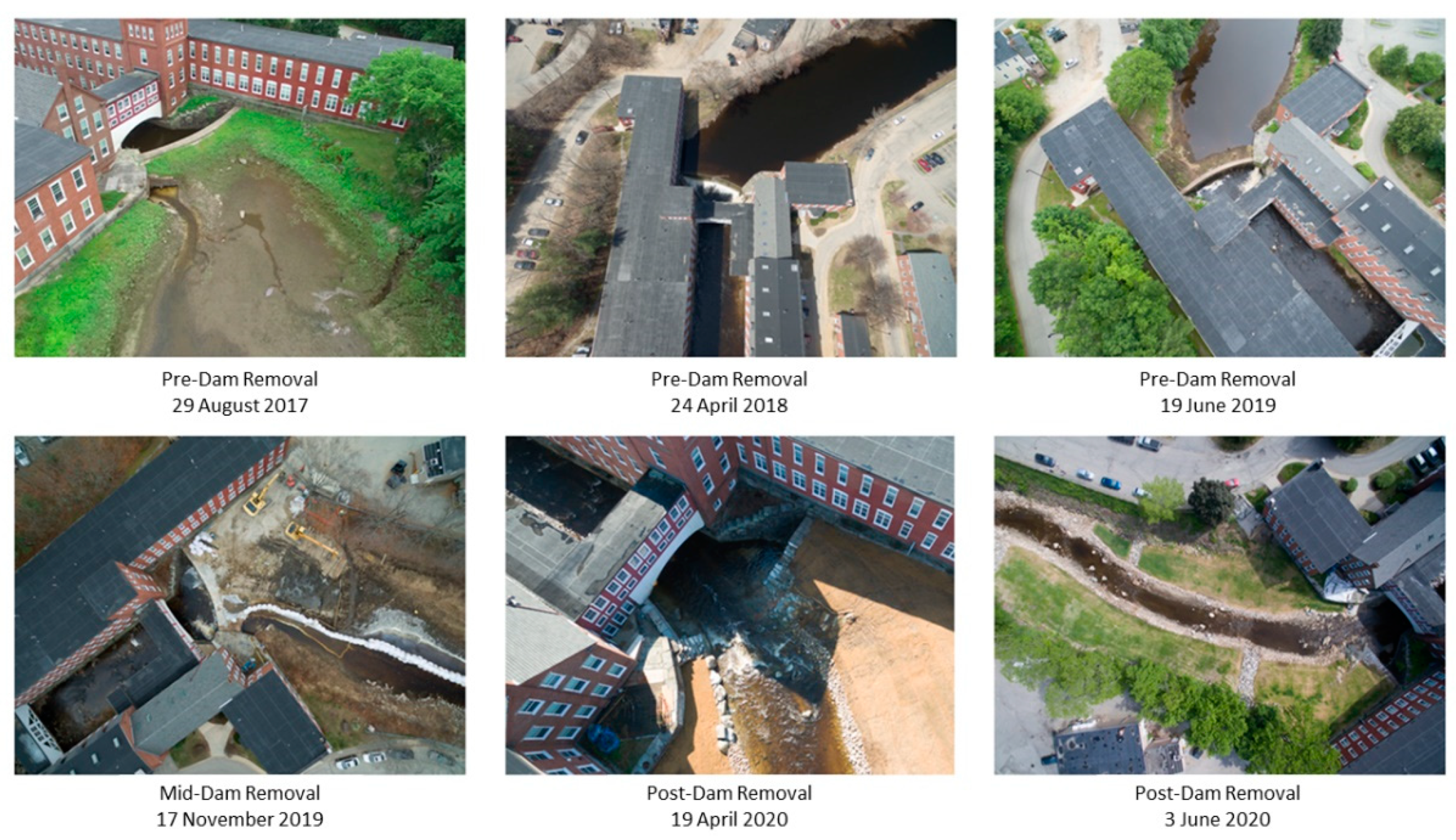
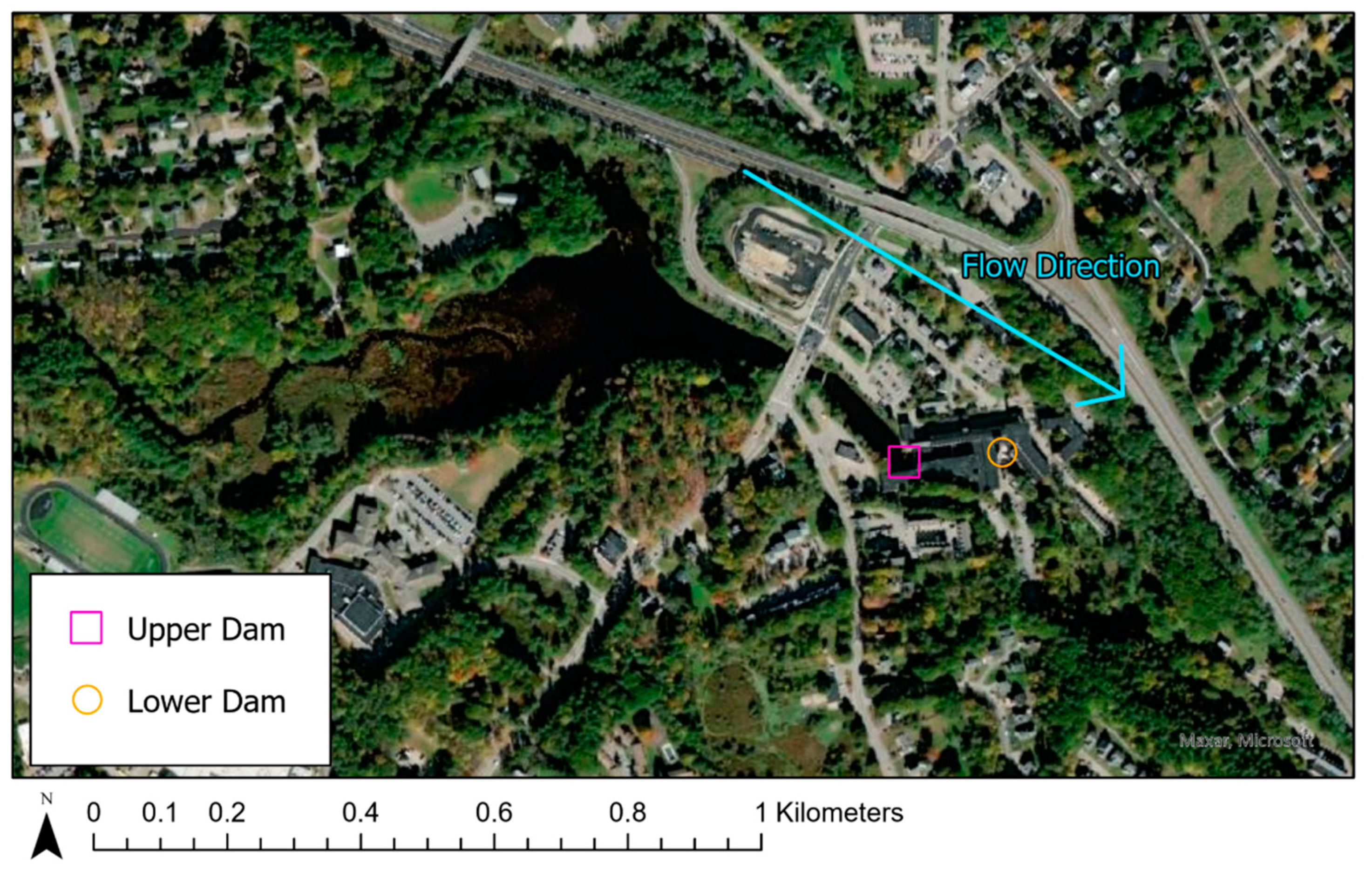
2.1. Study Setting Background: The Sawyer Mill Dam Removals

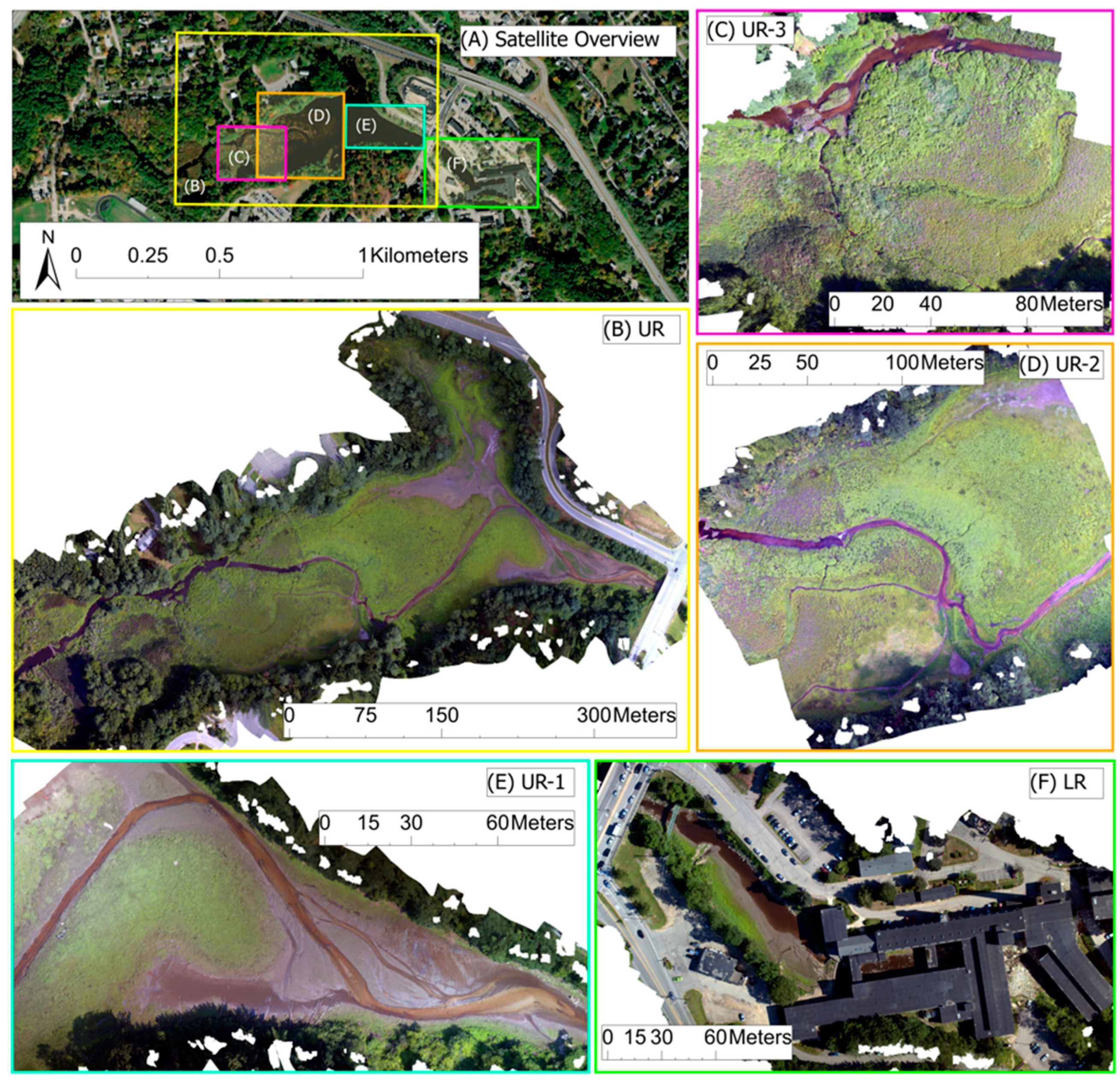
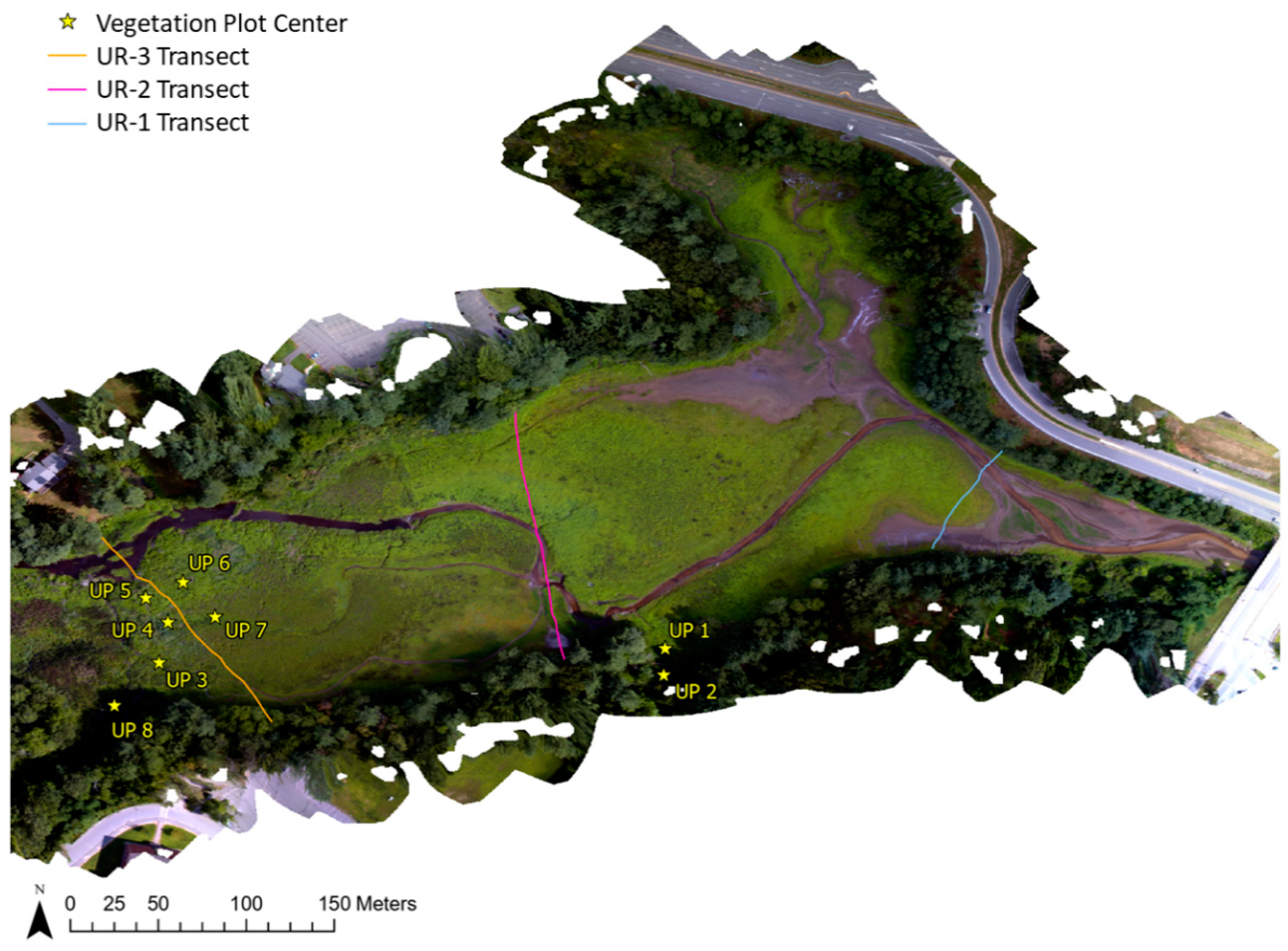
Two privately owned dams were located on the Bellamy River at the Sawyer Mill Apartments (Dover, NH, USA; Figure 1). We refer to them herein as the upper dam (20.4 m long, 3.6 m high), located furthest upstream, and the lower dam (19.5 m long, 3.3 m high), located downstream [55]. The New Hampshire Department of Environmental Services (NHDES) Dam Bureau issued a Letter of Deficiency in December 2009 requiring both dams to pass 250% of the 100-year flood. The goals of the dam removal project included both safety and restoration aspects: (1) to resolve NHDES dam safety deficiencies by dam removals sufficient to eliminate them from Dam Bureau jurisdiction, and (2) to remove the dams to restore river function, including sediment and nutrient transport, water quality, and aquatic organism passage [56]. Stop logs were removed from the gate house of the upper dam on 8 September 2012 to dewater the reservoir for topographic survey as well as begin the establishment of vegetation to help stabilize sediment. Post-stop log removal, the reservoir was periodically inundated when the capacity of the gate was exceeded, which was observed to be largely a seasonal occurrence.

Contractors used active sediment management strategies that included dredging for both dam removals. Levels of contaminants (metals, polycyclic aromatic hydrocarbons, polychlorinated biphenyls, and pesticides) that posed unacceptable ecological risk to downstream environments were found in the impounded sediment near the dams. Contaminant concentrations in sediment samples from the reservoir above the Route 108 bridge were significantly less than those from samples near the dams, so dredging was not implemented, and sediments were allowed to naturally erode from this area [57]. The lower dam removal was completed from 19 September 2018 to 31 December 2018. The upper dam removal was completed from 30 October 2019 to 31 March 2020 (Figure 2), and was the removal that triggered notable ecological changes in the reservoir. It was a relatively small dam removal that utilized active sediment management strategies, adding a relatively unique case study to the dam removal literature [2,24].

A small dam was located upstream of the Bellamy River Reservoir near Bellamy Park Disc Golf in Dover, NH. A larger drinking water reservoir dam, the Bellamy Reservoir dam, impounded the Bellamy Reservoir (impoundment area of 333 acres) in Madbury, NH further upstream of the disc golf course [58]. At the time of the Sawyer Mill dam removals, the lower dam was the first dam encountered moving upstream from the river’s mouth at Great Bay. The lower dam at Sawyer Mill had an impoundment area of approximately 0.4 acres and the upper dam had an impoundment area of approximately 22 acres.

2.2. Study Areas

We subset the Bellamy River Reservoir into five areas for river restoration monitoring (Figure 3). We treated the entire reservoir above the bridge as one area (“upper reservoir”; UR) and flew the UAV relatively higher to capture overall conditions of UR at a given sampling time (Figure 3B). We further divided UR into three smaller areas to conduct lower-flying-height, more detailed data collection. These three areas are described here in their pre-dam removal condition. The most upriver section of the reservoir (UR-3) contained beaver dams as well as relatively taller and shrubbier vegetation (woody and non-woody) than the other study areas (Figure 3C). A middle section of the reservoir (UR-2) was selected for its intersecting channel geomorphology and the presence of a large beaver dam and additional smaller beaver dams. The vegetation in UR-2 mainly consisted of large, fairly homogenous patches of herbaceous vegetation, non-woody shrubs, and little woody shrub vegetation (Figure 3D). The most downriver section of the reservoir just before the bridge (UR-1) consisted mainly of homogenous, short herbaceous vegetation and exposed sediment (Figure 3E). The “lower reservoir” (LR) was the area between the Route 108 bridge and the upper dam (Figure 3F). LR was estimated to contain 2294 cubic meters (3000 cubic yards) of sediment [57]. Contractors dredged LR and removed an estimated 1743 cubic meters (2280 cubic yards) of sediment during the upper dam removal (Kevin Lucey from NHDES, personal communication, email, 22 December 2020).

2.3. Fieldwork

2.3.1. UAV Flights

We photographed the study areas pre- and post-dam removal with a DJI Phantom 3 Professional (P3P) UAV equipped with its original RGB camera (

Table 1. Summary of Fieldwork. Imagery collection dates and accompanying boots-on-ground fieldwork. “Number of Images” column lists how many photos were uploaded into PhotoScan for the SfM process from the flight date. Vegetation plot centers were surveyed on 6 August 2019.

Study Area	Flight Date	Flying Height (m above Ground Level)	Number of Images	Topographic Survey Data	Comparable Vegetation Plot Data?
UR	14 August 2019	76	495	CPs, Transects surveyed on 1: 30 July 2019; 1 August 2019; 6 August 2019 GCPs surveyed on: 19 July 2019; 30 July 2019; 6 August 2019	Yes
	10 July 2020		496	CPs, Transects surveyed on1: 16 July 2020; 24 July 2020 GCPs surveyed on: 29 April 2020; 3 May 2020; 8 May 2020	No
UR-3	22 August 2019	46	288	CPs, Transects surveyed on: 22 August 2019 GCPs surveyed on: 6 August 2019	Yes
	6 August 2020		288	CPs, Transects surveyed on: 7 August 2020 GCPs surveyed on: 8 May 2020	No
UR-2	23 August 2019	46	364	CPs, Transects surveyed on: 23 August 2019 GCPs surveyed on: 19 July 2019; 6 August 2019	Yes
	24 July 2020		365	CPs, Transects surveyed on: 24 July 2020 GCPs surveyed on: 3 May 2020	No
UR-1	30 July 2019	30	469	CPs, VCPs, Transects surveyed on: 30 July 2019; 1 August 2019 GCPs surveyed on: 19 July 2019; 30 July 2019	NA
	16 July 2020		460	CPs, VCPs, Transects surveyed on: 16 July 2020 GCPs surveyed on: 16 July 2020
LR	19 July 2019	61	289	For both LR dates: Opportunistic GCPs and VCPs surveyed on 19 July 2019; 9 August 2019; 11 September 2019 2; 22 May 2020	NA
	5 August 2020		289

¹ Survey measurements from lower-flying-height areas were applied to UR assessments if they were collected within approximately two weeks before or after the UR flight date. ² Total station measurements rather than Hiper Lite +; 1 VCP used for LR was surveyed with a Topcon Total Station using two of the Hiper Lite + measured points due to poor satellite signal in the downriver area of that reach (11 September 2019 measurement set). These total station measurements were primarily collected for separate work not presented herein.

; see P3P documentation from DJI for details on camera specifications) [59]. We equipped a polarizing filter to the camera to help reduce glare from the water’s surface. The sampling times herein were limited to summer to capture seasonal herbaceous cover and provide lower flow conditions to minimize known complications associated with SfM-derived bathymetry, such as effects of deeper water, water turbulence, and water turbidity [33,60,61]. All nadir imagery was collected using automated flight paths with a set flying height above ground level and sufficient image overlap for SfM (90% forward overlap and 80% side overlap). Angled imagery (20 degrees off-nadir) was collected to supplement the nadir imagery to improve the accuracy of SfM models and prevent model deformation [62,63,64].

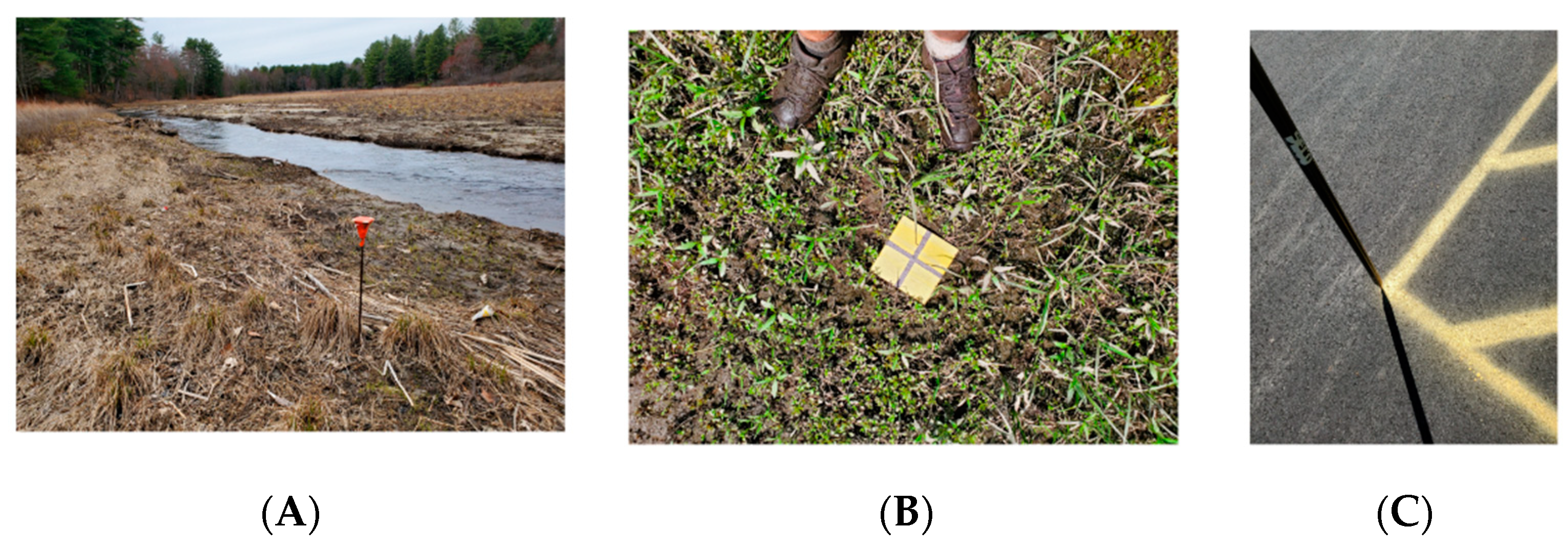
2.3.2. Topographic Measurements

Data collection that accompanied UAV flights frequently included field photographs taken from the ground and topographic measurements mainly completed with a GPS+ RTK Topcon Hiper Lite+ system (Table 1), with a rover and a base set over a known point [65]. See S1, S2, and the Data Availability section for information on topographic data and processing. It is important in UAV workflows to have visibly distinguishable features with measured locations in study areas for georeferencing and processing the UAV imagery as well as for evaluating the UAV products’ topographic accuracy. We installed and surveyed ground control points (GCPs), with most markers created from rebar and orange rebar caps (Figure 4A), throughout UR with the goal of at least 15 GCPs per sub-area for use in SfM image processing following GCP layout design recommendations from Agüera-Vega et al. (2017) [66]. We did not install rebar at LR, but rather surveyed existing markings (e.g., painted parking lot lines) throughout the area to use as markers (Figure 4C). We surveyed additional markers throughout UR-1 (Figure 4B) and LR, the most easily navigable study areas on foot, during their sample times to serve as visual check points (VCPs). The Agisoft software uses GCP information to build the UAV products (DSM, orthomosaic, point cloud, etc.), therefore the GCP-based accuracy metrics reported by the software tend to provide an overly optimistic perspective of model topographic accuracy since those points were used to correct the model. VCPs, on the other hand, provide a topographic accuracy assessment separate from the GCPs within the Agisoft software, thereby providing a more realistic estimate of model accuracy (GCP and VCP implementation in Agisoft further discussed further in Section 2.4). The GCP configurations per area varied slightly across the sampling dates, but generally remained consistent by trying to distribute GCPs evenly across the site and not in lines [67,68,69]. Our VCP layout designs followed the same strategies recommended from previous literature for GCPs but with a smaller marker count [66,67,68,69].

In addition to GCPs and VCPs, we surveyed checkpoints (CPs) throughout the UR study areas across a variety of terrain types, and recorded terrain notes at each surveyed CP. CPs served as an additional topography accuracy assessment outside of the Agisoft software (discussed in Section 2.5) and provided reference data for training and evaluating vegetation classification algorithms (discussed in Section 2.6). CPs were unmarked surveyed points throughout the landscape, unlike the physical markers in the field used for GCPs and VCPs. Vegetation CPs included accompanying vegetation height measurements made at the surveyed points. To record vegetation height, we generally used a tape measure placed from the bottom of the survey rod extended to the height of the vegetation closest to the rod. Vegetation height measurements were collected for all herbaceous and shrub species encountered while collecting CPs. Tree heights were not measured in the field. The CPs were surveyed throughout the areas with some bias due to site navigability (e.g., CPs concentrated in and around the stream channel). However, we made efforts to try to capture the heterogeneity of the landscape by collecting CPs in these broad categories (if applicable) throughout the extent of the areas: vegetation (herbaceous and shrub cover), dry terrain (e.g., logs, exposed sand or gravel), and wet cover (e.g., points within the streambed). The number of CPs collected per study area sampling time varied (e.g., from 61 CPs collected for the UR-1 30 July 2019 sampling time to 274 CPs collected for the UR-1 16 July 2020 sampling time, see Data Availability section for details). CP collection was more opportunistic as we navigated the site for fieldwork tasks in 2019 and became more systematic in 2020 (e.g., walking 10 or 15 step intervals in the stream channel in UR-1 and UR-2 and collecting CPs across the different categories at each interval) to better ensure site coverage and to collect water’s edge points to enable refraction correction methods in potential future work.

We surveyed transects in conjunction with flight times by walking a set number of steps (5 or 10 step intervals) and surveying points between stakes driven at the far ends of the reservoir (Figure 5). Smaller step intervals (3 steps) were sometimes used in the stream channel to provide more surveyed points in wet cover for comparison to the UAV DSMs or to capture features such as bars if present. The transects were primarily collected for comparison to the UAV DSM results, but we intended for them to also serve as geomorphic measures by collecting measurements along the same transect lines pre- and post-dam removal to capture channel shape changes. We placed the transects one per lower-flying-height area to cover the extent of UR and keep track of features that could change post-dam removal (e.g., large beaver dam in UR-2). We noted terrain type and vegetation height (if applicable to the point) at each surveyed transect point like we did with the CP measurements.

2.3.3. Vegetation Plots

We placed vegetation plots haphazardly along the transects established within UR in areas that received frequent inundation and were dominated with hydrophytic vegetation adapted to the fluctuating hydrology. We anticipated the vegetation communities in these areas would respond with the rapid changes in hydrology expected to occur following dam removal. Given the periodical inundated conditions within UR prior to dam removal, we were limited to establishing the vegetation plots in areas where most herbaceous vegetation could be assessed in the western portion of UR (Figure 5). We sampled the vegetation plots in August 2019 following methods outlined in the Stream Barrier Removal Monitoring Guide (SBRMG) [1]. The COVID-19 pandemic prevented vegetation plot sampling in 2020. We used an illustrative percent cover guide in the field to estimate percent cover for each species. Species’ coverages were noted as cover classes (Appendix A). Our definitions for vegetation structure were adapted from the SBRMG as follows: herbaceous cover was vegetation less than 0.9 m (3 ft) in height, shrub cover was 0.9 m (3 ft) to 6.1 m (20 ft), and tree cover was >6.1 m (20 ft). Herbaceous plants were evaluated within a 1.5 m (5 ft) radius from a vegetation plot center, shrub plants within a 4.5 m (15 ft) radius, and tree cover within a 9 m (30 ft) radius. To calculate total vegetation cover values for each vegetation structure class, we summed the estimated cover for the species in each structure class according to their cover class ranges to provide the range of total vegetation cover for each structure class per plot. Then, we averaged the total high and low values for each structure layer per plot to provide a mean cover estimate.

2.4. Structure from Motion

We processed the UAV imagery in Agisoft PhotoScan Professional version 1.4.x to create orthomosaics and DSMs for each study area flight date in Table 1 [31]. In general, the SfM workflow consisted of: (1) adding raw photo files for a flight date to a PhotoScan project, (2) letting image EXIF data autofill camera calibration parameters, (3) estimating images’ quality and disabling photos with a quality index below 0.5, (4) aligning the images to create a sparse point cloud model (a 3D representation of the tie point data, where tie points are matches between key points detected on two or more different images), (5) georeferencing the model by marking GCPs (and VCPs, if applicable) in images and inputting their surveyed coordinates, (6) optimizing camera positions based on GCPs, (7) building the dense point cloud (a 3D representation of dense point data, which is produced by calculating depth information for each camera to be combined into a single dense point cloud based on the estimated camera positions), (8) building the DSM (a 2D raster where the cell values represent surface elevations, in this case rasterized from the dense point cloud data), (9) building the mesh (a 3D polygonal mesh model, in this case constructed from the dense point cloud data), (10) performing color calibration across the images based on the mesh, and (11) building the orthomosaics (a mosaic of orthorectified images, where orthorectified images are geometrically corrected aerial photographs such that the scale is uniform). We exported the orthomosaic and DSM for each flight date along with a processing report, which included topographic accuracy metrics based on the GCP and VCP (if applicable) markers. VCPs are marked in the aerial imagery in the same way as GCPs in the Agisoft software. However, VCPs are “unchecked” during processing to reserve them for separate accuracy assessments while GCPs are “checked” to indicate their use in georeferencing and other processing steps. The general workflow, from adding photos to the project to exporting the products, is outlined in the PhotoScan manual, and we refer readers to this document to familiarize themselves with SfM photogrammetric processing [31]. Details of the parameters used in each step of the SfM workflow in PhotoScan are in S3.

2.5. Evaluating the Z Accuracy of the DSMs by Terrain Type

In addition to the GCP- and VCP-based topographic accuracy metrics reported by PhotoScan, we examined the accuracy of the DSMs relative to the CP and transect data across a variety of terrain types. We extracted the DSM values at the XY locations of the surveyed CPs and transect points in GIS. Using the surveyed elevations and extracted DSM values across the available areas and flight dates (Table 1), we examined trends in the DSMs’ Z accuracy across different terrain categories: vegetation, dry terrain (e.g., exposed ground or wood), and submerged terrain (e.g., substrate). We overlaid the surveyed points on the corresponding orthomosaics to visually inspect and verify the terrain type of each point noted in the field against the conditions at the time of imagery capture.

2.6. Classifying Vegetation Structure

2.6.1. Classification Methodology and Thematic Accuracy

We used the SfM products and ML to classify and quantify vegetation structure cover throughout the reservoir and evaluate changes pre-/post-dam removal. The classification schema consisted of four classes: three vegetation structure classes that followed the same height definitions for herbaceous (“herb”), shrub, and tree cover based on the SBRMG, and an “other” class that represented non-vegetative cover.

We used the support vector machine (SVM) algorithm in ArcGIS Pro along with a 2-band raster featureset made from the SfM products for classifying vegetation structure in study areas with ground reference data, where ground reference data were CPs and transect points with accompanying vegetation height measurements. One band of the raster featureset represented Green Leaf Index (GLI) values and one band represented DSM elevation values (hereafter referred to as “GE” featuresets, “G” for GLI and “E” for elevation). An advantage of the SVM algorithm is its insensitivity to the amount of training data, which can make it a good choice for classification tasks with limited training samples [70,71,72]. The algorithm has been successfully used in vegetation mapping applications [53]. We trained eight SVM classifiers, each specific to one sampling time’s ground reference data and GE featureset. We could not collect ground reference measurements in LR’s stream environment due to site access restrictions, and therefore did not classify vegetation structure at LR.

We reasoned that the GE featureset contained the basic information for the SVM to classify vegetation structure: a vegetation index to help separate vegetative cover from non-vegetative cover, and elevation information to help distinguish between vegetation structure types assuming the landscape was relatively flat [73]. We calculated GLI values across each orthomosaic using their red, green, and blue band digital values [74]:

GLI = (2 × Green − Red − Blue)/(2 × Green + Red + Blue).

(1)

We chose to use this index over other visible vegetation indexes since there is evidence that it is better for highlighting vegetation compared to the visible atmospherically resistant index and the visible atmospherically resistant indices green [75]. GLI values range from −1 to 1. Negative GLI values tend to be soil/non-living cover while positive values are green leaves and stems [74]. We rescaled the values of each GLI and DSM raster band from 0 to 100 using linear min–max rescaling to make their magnitudes comparable. The rescaled GLI and elevation bands composited together formed each GE featureset.

We manually digitized sample polygons, based on the ground reference data and visual interpretation of the orthomosaics and DSMs, to train and evaluate the SVM classifiers. We did not measure tree heights in the field, but tree cover was visually discernible in the orthomosaics and DSMs for digitization. We digitized a total of seven training polygons per class and three test polygons per class per sampling time. We used GE featureset values within the training sample polygons to train each SVM classifier. A maximum of 500 samples (pixels) per class were drawn from across the training polygons for training. We used each GE featureset and its corresponding trained SVM classifier to classify the pixels across the entire featureset, providing a map of vegetation structure throughout an area at a given sampling time. We evaluated the SVM classifiers’ accuracies by drawing 500 test samples (pixels) per class from each set of test polygons and classified results to compute confusion matrices, Kappa statistics, and overall accuracy values. The Kappa statistic levels of agreement were interpreted following McHugh (2012) [76]. The tools in ArcGIS Pro used to complete this classification workflow included (1) the “Raster Calculator” tool, “Rescale by Function” tool, and “Composite Bands” tool to create the GE featuresets from the DSMs and orthomosaics, (2) the “Training Samples Manager” tool to digitize the train and test polygons, (3) the “Train Support Vector Machine” tool for training each SVM classifier, and (4) the “Create Accuracy Assessment Points”, “Update Accuracy Assessment Points”, and “Compute Confusion Matrix” tools for the thematic accuracy assessment. Comparable tools in other GIS software could also be used to complete the workflow.

2.6.2. Landscape-Level Results and Comparison to Boots-on-Ground Vegetation Plot Data

We used the classified vegetation maps in GIS to calculate percent cover of each class in manually digitized vegetation assessment areas that encompassed each UR study area, providing estimates of landscape-level changes. We also compared the results from the UAV approach to the conventional vegetation plot data. To do so, we replicated the vegetation plot radii used for in-field assessments in GIS by buffering the surveyed plot center locations following the SBRMG assessment radii for each vegetation structure type. We calculated percent cover of each vegetation structure class according to the classification results for each plot’s corresponding assessment radii and compared them to the in-field mean structure cover estimates. The summer 2019 classification results were used for each study area to match when the in-field vegetation data were collected (Table 1). In addition, we compared the UR classification results to the UR-3 results relative to in-field vegetation plot data to gain perspective of how flying height and ML training sample distribution may have impacted the classification results.

2.7. Mapping and Quantifying Geomorphic Change

2.7.1. Creating DSMs of Difference and Vegetation Masks

We used SfM to map relative erosion and deposition and estimate sediment volume changes post-dam removal by creating DSMs of difference (DoDs), which are made by subtracting one DSM from another (we used the “Raster Calculator” tool available in ArcGIS Pro) and show elevation changes for each study area. Mapping vegetation was useful for removing its influence from geomorphic assessments, helping to minimize topography changes associated with vegetation rather than earth in the SfM DoDs. RGB vegetation indices can classify and remove vegetation in SfM point clouds to make digital elevation models representing bare earth from DSMs with vegetation cover [77]. However, using this approach at sites with dense vegetation cover throughout the area, such as the UR study areas, would result in many points being removed across the landscape. Instead, we created vegetation masks from the UAV classification results for each of the DoDs’ most recent sampling date that masked vegetation cover from each DoD. A visually estimated GLI threshold was used to create a vegetation mask for the LR DoD since no classification data were available. Creating the vegetation masks in GIS involved using the “Raster Calculator” tool to create binary rasters that distinguished vegetation cover (combined “herb”, “shrub”, and “tree” classes) from non-vegetation cover (other class), converting the binary raster to polygons using the “Raster to Polygon” tool, and deleting the polygons with values that were not to be included in the mask (polygons that represented the “other” class).

2.7.2. Adding Minimum Level of Detection Threshold Masks

The changes shown in DoDs can be a result of the DSMs’ spatial error and not true topographic change. Marteau et al. (2017) and Brasington et al. (2003) used the following equation to calculate minimum level of detection (minLoD) thresholds to detect significant, low magnitude geomorphic changes in DoDs [38,78]:

$$minLoD=\mathrm{t}\sqrt{{\left(\mathsf{\epsilon }DS{M}_1\right)}^2+{\left(\mathsf{\epsilon }DS{M}_2\right)}^2},$$

(2)

where Z₂ and Z₁ are the elevation in a given cell of the most recent and older DSM, respectively, εDSM₂ and εDSM₁ are their respective error terms, and $\mathrm{t}$ is the critical t-value at the chosen confidence level. If the difference in elevation between two DSMs in a given cell (Z₂ − Z₁) was smaller than the $minLoD$ threshold, then the change was considered uncertain at the chosen confidence interval following Marteau et al. (2017) [38]. Their approach was adapted for this study by using marker error metrics reported by PhotoScan; GCP error metrics were used when no VCP data were available for a sampling time. The standard deviation of each GCP or VCP marker set’s Z error was calculated for each sampling time and used as the $\mathsf{\epsilon }DSM$ variables. A critical value ($\mathrm{t}$) of 1.96 was used in Equation (2) for a 95% confidence interval.

We made minLoD masks from binary rasters that represented absolute elevation differences from the DoDs that were either greater than or less than the minLoD values. Making the minLoD masks in GIS involved using the “Raster Calculator” tool to create the binary rasters, the “Raster to Polygon” tool, and then deleting the polygons not to be included in the mask (polygons that represented areas that had absolute elevation differences greater than the minLoD threshold). The vegetation and minLoD masks were merged using the “Merge” and “Dissolve” tools. The output was used in the “Symmetrical Difference” tool in conjunction with a large manually digitized polygon that covered the DoD extent. Then, the output from the “Symmetrical Difference” tool along with manually digitized geomorphology assessment area polygons were used to clip the DoD rasters so that only non-vegetated, significantly changed areas of the DoDs within the assessment areas had raster values. These “fully masked” DoDs visualized the spatial distribution of erosion and deposition post-dam removal.

2.7.3. Calculating Volume Changes within Geomorphic Assessment Areas

We created rasters representing volumetric change per pixel rather than elevation change by multiplying the values of the fully masked, clipped DoDs by the surface area represented by each pixel when projected using NAD 1983 (2011) StatePlane New Hampshire FIPS 2800 (Meters), allowing us to estimate in GIS the volumes of erosion, deposition, and net change each geomorphology assessment area experienced post-dam removal. We ignored the influence of changing woody debris on the geomorphology assessments in this study, as mapping woody debris was outside the scope of this work and was treated as “other” cover in the classification schema. The assessment area polygons for the geomorphic assessments were drawn to avoid obvious large woody debris (e.g., fallen trees) and overhanging branches.

3. Results

3.1. UAV Model Topographic Accuracy

3.1.1. GCP- and VCP-Based Topographic Accuracy Metrics from PhotoScan

The orthomosaics, DSMs, and PhotoScan processing reports used herein are in the Data Availability section along with other items such as the UAV photos, and boots-on-ground topographic and vegetation plot data. Error in PhotoScan is the difference in the corresponding coordinate (X, Y, Z) between the surveyed marker location and the estimated marker location from SfM. According to these metrics included in the PhotoScan processing reports, the largest error most frequently came from the Z coordinate in the UAV models used for monitoring restoration impacts in the Bellamy River Reservoir (

Table 2. GCP and VCP Error Metrics. GCP and VCP error metrics from the processing reports generated by PhotoScan, which are the root-mean-square error for all the GCP or VCP markers for each coordinate. “Total” implies averaging over all the GCP locations or VCPs [31].

Study Area	Flight Date [dd/mm/yyyy]	Number of GCPs	X GCP Error (cm)	Y GCP Error (cm)	Z GCP Error (cm)	Total GCP Error (cm)	Number of VCPs	X VCP Error (cm)	Y VCP Error (cm)	Z VCP Error (cm)	Total VCP Error (cm)
UR	14 August 2019	27	3.42	3.08	3.39	5.71	NA	NA	NA	NA	NA
	10 July 2020	27	3.27	3.28	3.78	5.98	NA	NA	NA	NA	NA
UR-3	22 August 2019	14	1.74	1.93	2.07	3.32	NA	NA	NA	NA	NA
	6 August 2020	12	1.07	1.76	5.02	5.43	NA	NA	NA	NA	NA
UR-2	23 August 2019	19	3.46	8.53	4.39	10.20	NA	NA	NA	NA	NA
	24 July 2020	19	1.65	1.49	3.31	3.98	NA	NA	NA	NA	NA
UR-1	30 July 2019	15	1.92	2.26	5.57	6.31	9	5.95	6.61	6.28	10.89
	16 July 2020	15	1.56	2.37	4.72	5.51	9	1.39	1.66	3.28	3.92
LR	19 July 2019	20	4.91	4.78	6.37	9.35	10	6.55	6.47	6.66	11.36
	5 August 2020	20	5.36	5.02	5.68	9.28	9	6.42	5.16	6.88	10.73

).

3.1.2. CP-Based Z Accuracy Evaluation by Terrain Type

The terrain-specific topographic assessments performed in GIS revealed that dry, unvegetated surfaces tended to be modeled the most accurately in the UAV DSMs relative to the boots-on-ground CP and transect point measurements while the elevations of vegetated surfaces tended to be underestimated (lower than actual) and elevations of wet (submerged) surfaces tended to be overestimated (higher than actual) (Figure 6;

Table 3. Surveyed vs. UAV Z Error Statistics by Terrain. Z error statistics for the DSMs across terrain categories using the transect point and checkpoint measurements as reference.

Relative Flying Height	Terrain Type	Number of Points		Elevation from DSM (m) - (Surveyed Elevation + Vegetation Height Noted in Field (m))
				Average	Median	Minimum	Maximum	St. Dev.	RMSE
Low 1	Dry	109	0.003		0.006	−0.182	0.231	0.066	0.066
	Wet	362	0.213		0.145	−0.135	1.499	0.240	0.321
	Vegetation	414	−0.135		−0.072	−1.899	0.608	0.277	0.308
High 2	Dry	101	−0.031		−0.042	−0.243	0.152	0.067	0.074
	Wet	225	0.225		0.131	−0.124	1.257	0.252	0.338
	Vegetation	232	−0.204		−0.215	−1.308	0.682	0.259	0.330

¹ “Low” relative flying height refers to Z measurement comparisons made using the UR-1, UR-2, and UR-3 DSMs with the surveyed points for those flight dates; ² “High” relative flying height refers to Z measurement comparisons made using the UR DSMs with surveyed measurements that were within approximately 2 weeks before or after the UR flight dates.

). We show the higher-flying-height results separately from the lower-flying-height results (Figure 6; Table 3) since the time difference between the ground reference data collection and flights increased the uncertainty associated with the higher-flying-height elevation differences (Table 1).

3.2. Boots-on-Ground Vegetation Plot Data vs. UAV Classified Vegetation Cover

The UAV vegetation classification approach tended to underestimate herbaceous cover and overestimate shrub cover relative to the in-field vegetation plot data, while tree cover estimates were more comparable between the two methods (Figure 7). The lower-flying-height classification results with ML training samples more concentrated around the plot locations generally provided more comparable estimates of vegetation cover relative to the in-field plot data than the higher-flying-height results with ML training samples distributed throughout UR (Figure 8). The lower-flying-height UR-2 classification results were not compared to the higher-flying-height UR results (Figure 8) or included in the more general UAV vs. conventional plot results comparison (Figure 7) because the two plots in UR-2 were located towards the edge of the UAV products where the quality of the modeled surface was compromised due to lack of overlapping images (S4). Appendix A contains the in-field, structure-level vegetation plot results.

3.3. Landscape-Level UAV Vegetation Structure Cover Results

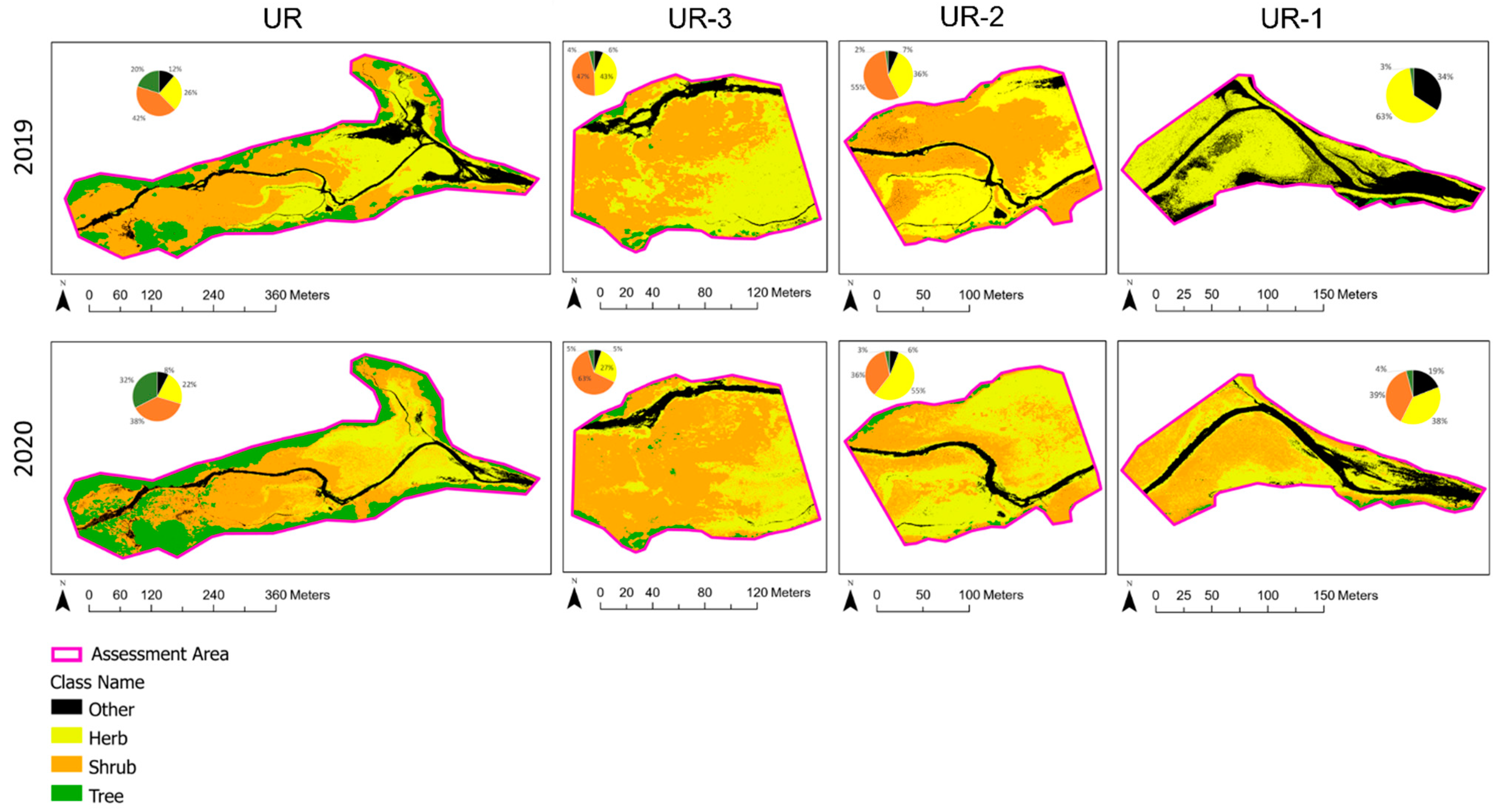
3.3.1. Landscape-Level Vegetation Maps Pre-/Post-Restoration and Complications

The lower-flying-height flight paths for UR-3, UR-2, and UR-1 resulted in some DSM local distortions in tree cover, explained by insufficient image overlap for SfM due to the UAV’s fixed flying height above ground level relative to the height of the tree canopy surface (Figure 9). Areas affected by local distortions were often misclassified. According to the UAV vegetation maps (Figure 10), UR experienced an increase in vegetation cover as a whole (decrease in “other” cover) and a decrease in herbaceous cover in most of the study areas, with the replacement of herbaceous cover with shrub cover noticeably observed in UR-3 and UR-1. These changes were supported by field observations. An increase in tree cover was observed in the UAV results for the most upriver area of UR (Figure 10). However, this new “tree” cover was likely a result of classification inaccuracy. It would take longer than a year for trees to grow in the floodplain following dam removal, but vegetation could have grown taller or other taller species could have established. The misclassified tree cover may have been due to elevation anomalies in the training samples provided to the 2020 UR SVM (Figure 11). There was an increase in overlap between the elevation values for the tree and other vegetation classes in the 2020 training samples compared to the clear separation in the 2019 training samples.

3.3.2. Thematic Accuracy of Vegetation Classification Results

The accuracy metrics calculated from the test samples indicated that the vegetation structure maps were acceptably accurate (

Table 4. Accuracy Metrics of UAV Vegetation Classifications. Kappa statistics and overall accuracies for the vegetation classification results calculated from the test samples. Full confusion matrices are available in Appendix B.

Study Area	Flight Date [dd/mm/yyyy]	Kappa Value	Kappa Interpretation (Following McHugh 2012)	Overall Accuracy
UR	14 August 2019	0.98	Almost perfect agreement	99%
	10 July 2020	0.90	Strong agreement	92%
UR-3	22 August 2019	0.98	Almost perfect agreement	98%
	6 August 2020	0.77	Moderate agreement	83%
UR-2	23 August 2019	0.89	Strong agreement	92%
	24 July 2020	0.99	Almost perfect agreement	99%
UR-1	30 July 2019	1.00	Almost perfect agreement	100%
	16 July 2020	0.85	Strong agreement	89%

), with overall accuracies ranging from 83% to 100%. According to the confusion matrices (Appendix B), most confusion generally occurred between the herbaceous and shrub classes.

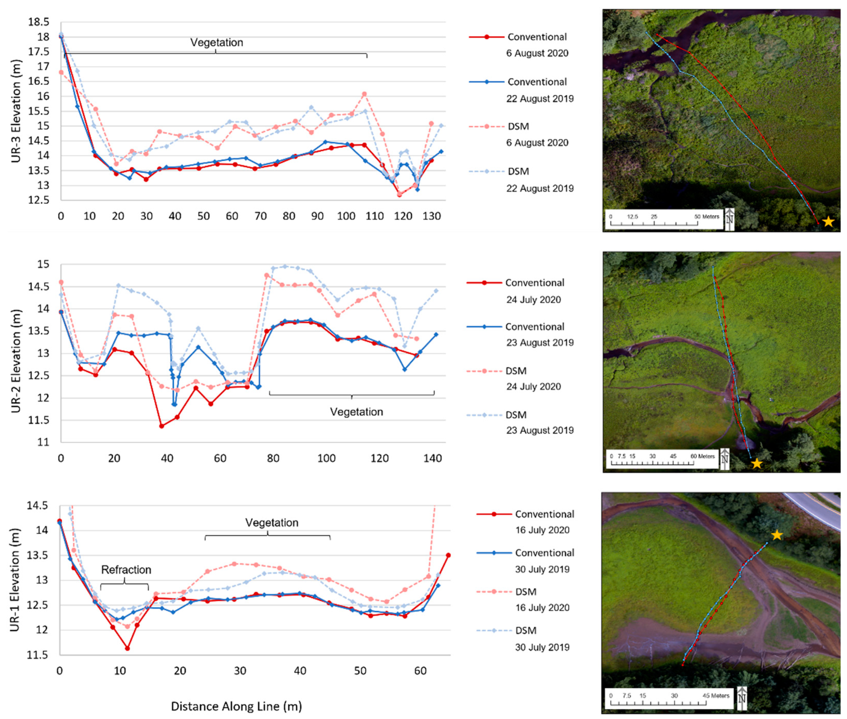
3.4. Boots-on-Ground Transects vs. UAV DSMs for Evaluating Post-Restoration Channel Changes

The surveyed transects provided elevation profiles showing differences pre-/post-dam removal (Figure 12). Due to insufficient overlap between the 2019 and 2020 surveyed paths for UR-3 and UR-2, it was inconclusive whether the changes shown were true geomorphic changes or simply different areas being surveyed each sampling time. The paths for UR-2 and UR-3 were challenging to consistently navigate on the ground due to changes in channel shape between 2019 and 2020, the taller vegetation obscuring the view of the end locations of the paths, and the more complicated channel intersections at UR-2. The surveyed paths for the UR-1 transect were more consistent as it was easier to precisely walk the survey path across the relatively simpler terrain. Therefore, elevation differences captured in this transect more likely reflect true geomorphic change. Based on the reliable transect, UR-1 experienced erosion in the instream channel and deposition on its bank following dam removal. The conventional transects also provided data to illustrate elevation differences between the surveyed ground and the DSM elevations extracted from the same XY locations (Figure 12), such as where vegetation cover influenced the DSM elevations to be higher than the ground or where refraction influenced the DSM elevations to be higher than the streambed. These comparisons illustrate why it was necessary to try to minimize the influence of vegetated cover from the DoDs via the vegetation masks. Despite these influences, the same pattern of erosion and deposition in UR-1 observed in the surveyed transects was seen in the DSM transects (Figure 12).

3.5. Landscape-Level UAV Geomorphic Change Results

3.5.1. Post-Restoration Erosion and Deposition Mapped from Masked DoDs

Through the fully masked DoDs (minLoD thresholds used in the masks are presented in

Table 5. Standard Deviations of Z Errors and minLoDs. The standard deviation of each sampling time’s VCP or GCP marker set’s Z errors report-ed by PhotoScan. The standard deviations were used as the εDSM variables in Equation (2) to provide the minimum level of detection threshold for each DoD.

Study Area	Sampling Date	VCPs or GCPs Used	Standard Deviation of Z Errors (cm)	Minimum Level of Detection Threshold (cm)
UR	10 July 2020	GCPs	3.78	9.94
	14 August 2019	GCPs	3.39
UR-3	6 August 2020	GCPs	5.02	10.65
	22 August 2019	GCPs	2.07
UR-2	24 July 2020	GCPs	3.31	10.77
	23 August 2019	GCPs	4.39
UR-1	16 July 2020	VCPs	3.10	11.16
	30 July 2019	VCPs	4.78
LR	5 August 2020	VCPs	6.85	18.72
	19 July 2019	VCPs	6.66

), we observed that erosion occurred throughout the instream environments of UR and LR (Figure 13) with some deposition occurring on the banks of UR-1 (Figure 13D) and in the most-upriver instream area of UR (Figure 13A). The areas of erosion and deposition detected in the DoDs largely agreed with field observations (UR-2 erosion examples provided in Figure 14). For additional perspective, the upper dam was 12 feet (3.66 m) high. Elevation changes detected in the LR DoD in the area closest to the former upper dam site were approximately −3 to −3.8 m (Figure 13E). Visually inspecting the UR orthomosaics revealed that the upriver deposition was related to beaver activity outside of our lower-flying-height study areas (Figure 15).

3.5.2. Post-Restoration Volume Changes within Geomorphic Assessment Areas

All study areas experienced net erosion following dam removal, while UR-1 experienced the most deposition and UR-2 experienced the most erosion of the lower-flying-height areas (

Table 6. Sediment Budgets. Sediment budgets for the assessment areas calculated from the masked DoDs. Figure 13 illustrates the assessment areas. “DoD Pixel Size” refers to the projected pixel sizes (in NAD 1983 (2011) StatePlane New Hampshire FIPS 2800 (Meters)) used for calculating volume change.

Study Area	More Recent Sample Time	Older Sample Time	DoD X and Y Pixel Size (m)	Erosion (m3)	Deposition (m3)	Net Change (m3)
UR	10 July 2020	14 August 2019	0.05382	2715.9	346.8	−2369.1
UR-3	6 August 2020	22 August 2019	0.03368	406.5	0.6	−405.9
UR-2	24 July 2020	23 August 2019	0.03426	957.8	5.6	−952.2
UR-1	16 July 2020	30 July 2019	0.02290	428.5	32.7	−395.8
Lower-Flying-Height Areas Together 1	See Above	See Above	See Above	1792.8	38.9	−1753.9
LR	5 August 2020	19 July 2019	0.04534	1024.0	7.5	−1016.5

¹ “Lower-Flying-Height Areas Together” reflects the sums of erosion, deposition, and net change across UR-1, UR-2, and UR-3. This provides a more conservative estimate of change focused on sections of the stream environment rather than the entire UR.

).

4. Discussion

4.1. Differences in UAV Model Topographic Accuracy across Terrain Types

We expected that wet (submerged) areas’ elevations may be overestimated (higher than actual) in the DSMs due to refraction, and we observed this in the terrain-based elevation comparisons (Figure 6 and Figure 12, Table 3). However, we did not apply refraction correction methods to the DSMs due to limitations discussed later in Section 4.6. Leaf-off conditions can result in the underestimation (lower than actual) of vegetation height in SfM topography [30], but leaf-on conditions were captured herein. Instead, the underestimation of vegetated surfaces may be related to the “Aggressive” depth filtering option used when creating the dense point clouds. Points representing individual plants could have been removed in the SfM filtering process as outliers (information on filter options is in the PhotoScan manual [31]), resulting in a smoothing of the vegetation surface. Meneses et al. (2018) also noted that automatic removal of outliers during SfM processing could have eliminated points corresponding to Phragmites reeds and consequently caused deviations in the heights represented in their elevation models, suggesting that the underestimation we observed may be a limitation of using UAV SfM to model similar vegetation types (e.g., grasses and reeds) [79].

4.2. Landscape-Level UAV Vegetation Structure Assessment

4.2.1. Thematic Accuracy Metrics Indicated Reliable Results

The UAV vegetation classification results had acceptable Kappa statistics, with most sampling times having strong or almost perfect agreement between the classified result and test samples (Table 4) [76]. The overall accuracies of these results on average (94%; Table 4) were comparable to the overall accuracy (up to 95%) reported by Ahmed et al. (2017) for mapping forest, shrub, herbaceous, bare soil, and built-up cover using UAV multispectral data and an object-based ML classification approach [47]. Most confusion occurred between the herbaceous and shrub classes (Appendix B). This confusion is not unusual in remote sensing classifications, as shrub composition tends to resemble forest and herbaceous vegetation since many of the same species are included in multiple structure classes and transitional shrub stages often exist along a continuum from herbaceous to forest cover [47].

4.2.2. UAV Captured Post-Restoration Changes Such as Vegetation Colonization and Succession

The UAV vegetation cover maps showed signs of vegetation succession [4,10,16] in UR. Colonization of dewatered sediments by pioneer herbaceous vegetation was noticeably observed in UR-1 and UR-2. We expected colonization to occur, as colonization can take as little as one month following dam removal [10,14,15,16]. We also expected that herbaceous cover would give way to shrubs and taller vegetation as the floodplain matures, and signs of this succession were detected in a short amount of time (within approximately 1 year; Figure 10). Based on these observations, vegetation succession can be expected to continue as the channel in the former reservoir reaches an equilibrium state and natural flow regimes are restored [4,20,21,22]. However, we noted patches of invasive species in the field, such as Phragmites and Lythrum salicaria (e.g., Figures S17, S69 and S70; see vegetation plot data in Data Availability section), in UR that preceded dam removal. Mapping specific species was outside the scope of this work, but invasive species can influence succession processes [80,81,82] and can interrupt the development of vegetation communities at dam removal sites [16]. On the other hand, dam removal case studies have shown that coverage of invasive species may not expand as expected following removal [83], and that colonization by invasive species can be less than expected [84]. We are uncertain whether invasive species will arrest the vegetation community’s development at UR, as a longer study period and methods that mapped vegetation species would be required.

4.2.3. UAV Flight Date Differences Could Have Impacted Observed Changes

When considering the UR-3, UR-2, UR-1, and UR vegetation results together, the upper reservoir generally experienced an increase in shrub cover and a decrease in “other” cover (Figure 10), in line with what could be expected to happen at former reservoir post-restoration following vegetation succession patterns [4,10,16]. However, the difference in UAV flight dates across the study areas’ paired sampling times may have influenced the observed changes for specific study areas. For example, replacement of shrub with herbaceous cover was detected in UR-2′s classification results (Figure 10). UR-2 was flown 23 August 2019 and 24 July in 2020, which may have introduced some differences in vegetation heights throughout the season. Class confusion between herb and shrub cover could have also played a role in this unexpected replacement of shrub cover with herbaceous cover (Appendix B).

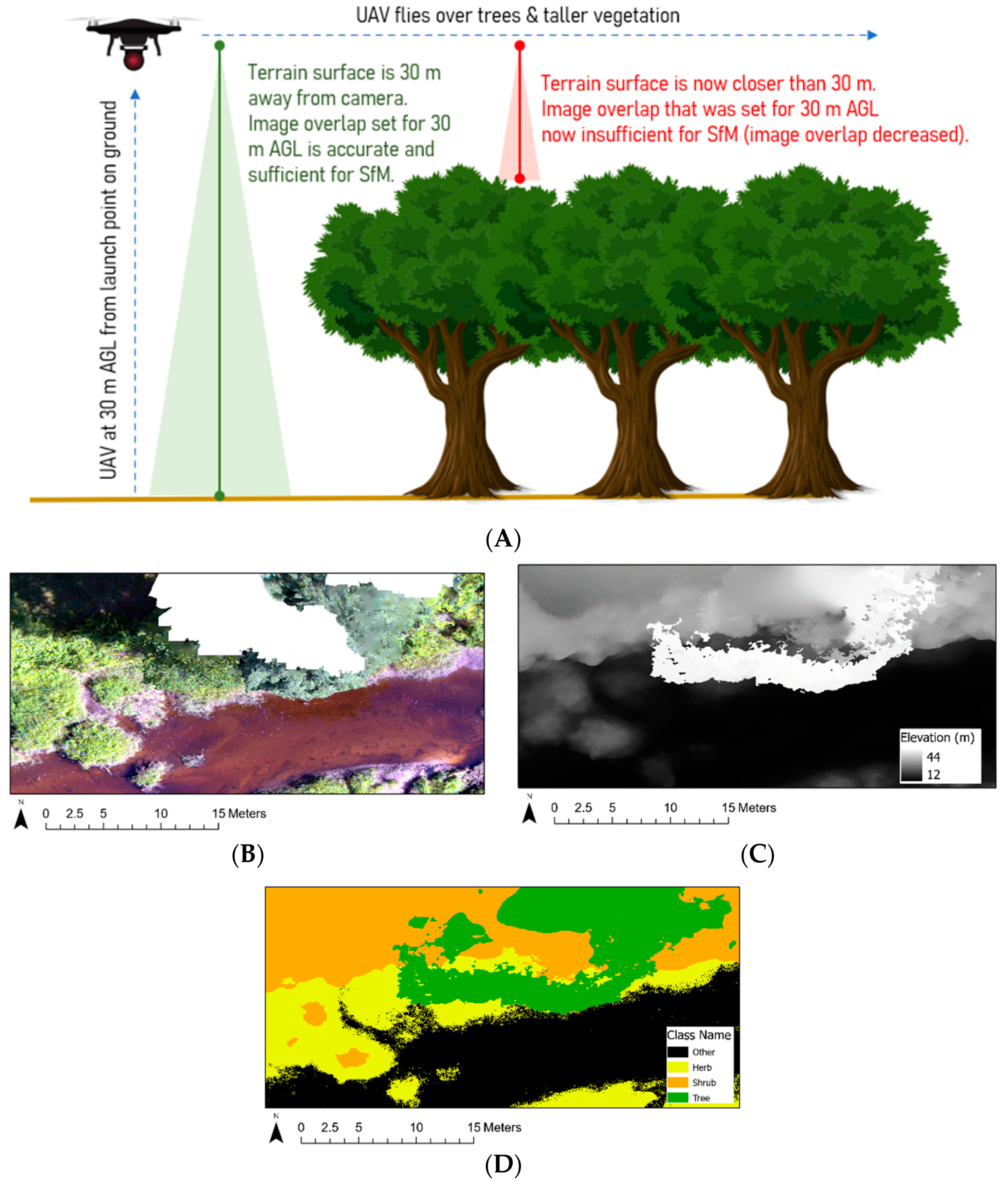
4.2.4. Considerations of Local Distortions in Canopy Cover

We observed some local distortions in tree cover in the DSMs related to image acquisition and SfM processing (Figure 9). Tree cover in the reservoir often existed on the edges of the areas that the UAV was programmed to capture, which increased the chance of DSM local distortions due to the fewer overlapping images of an area. These local distortions were often misclassified since the elevation values did not represent the actual tree canopy elevation (Figure 9D). This suggests that if tree cover is a priority for a restoration project, the UAV should be programmed to fly high enough over the tree canopy to capture sufficient image overlap for SfM.

Anomalies in DSM tree canopy (local distortions, Figure 9C; “holes”, S5) may partially explain why there was an estimated increase in tree cover in the UR results that was not observed in the field or in the orthomosaics (Figure 10). The 2019 UR training samples provided a clear distinction between the tree and other classes for the elevation feature (Figure 11). The 2020 tree training samples contained influences from DSM anomalies, resulting in outliers in the tree training elevation data and increasing overlap between classes for the elevation feature (Figure 11). Differences in the distribution of the training polygons throughout UR could have also played a role. The 2020 UR training polygons were drawn near UR-2 and UR-1 due to timing of ground reference measurements (Table 1). The 2019 training polygons were drawn across all three sub-areas. There is a slight upward slope throughout UR as you move upstream (difference of 2.4 or 2.7 m in the longitudinal profile from the Route 108 bridge to approximately 914 m upstream) [85], which suggests that the more limited distribution of training samples concentrated in the middle and downriver areas of UR could have impacted the robustness of the sampled elevation data applied across UR.

4.3. Comparing the Boots-on-Ground and UAV-Based Approaches for Vegetation Cover Assessment

4.3.1. UAV Provided a More Complete Perspective Than Spatially Limited Plots

The UAV maps provided more complete information on vegetation change than what would have been captured from the plots if we had been able to collect plot data in 2020, as much change occurred outside the plot radii. For example, much vegetation structure change was observed in UR-1 (Figure 10), which contained no plots (Figure 5). This demonstrates the advantage of using a landscape-scale approach rather than relying on vegetation plots with limited spatial coverage. This point was also emphasized by UR-2, where dewatered sediments outside of the main channel were colonized by herbaceous vegetation (Figure 10). The plots would have missed this due to their placement relative to the spatial extent of the colonization observed via UAV (Figure 5 and Figure 10).

The COVID-19 pandemic prevented us from collecting vegetation plot data in summer 2020. Our UAV enabled safe collection of post-removal vegetation data that would have been missed if relying solely on conventional vegetation plot data in this study. Completing fieldwork during the pandemic emphasized the importance of flexible and adaptive methods for successful restoration monitoring, such as those enabled via UAV.

4.3.2. Limitations of Using a Passive Sensor vs. Boots-on-Ground Investigation

In general, the UAV approach tended to underestimate herbaceous cover and overestimate shrub cover relative to the conventional plot data (Figure 7). The UAV camera was a passive sensor that could not penetrate the vegetation’s surface to detect herbaceous cover underlying taller vegetation classes, while botanists in the field could investigate for underlying herbaceous species. The UAV results’ overestimation of shrub cover was likely due to classification inaccuracies, particularly resulting from confusion between the shrub and herbaceous classes (Appendix B).

4.3.3. Classification Results from Lower-Flying-Height and Spatially Concentrated Training Samples Better Matched Plot Data

The classification results from the lower-flying-height imagery generally provided vegetation structure coverages more comparable to the boots-on-ground plot data than the higher-flying-height imagery (Figure 8). The training samples provided to the lower-flying-height UR-3 classifier were more concentrated around the plot locations and likely more reflective of the vegetation within the compared vegetation plots than the training samples provided to the UR classifier that were drawn throughout UR. These findings suggest that if there is a sub-area of a restoration project site where vegetation change is a primary concern, it may be worthwhile to conduct lower-flying-height assessments with ground reference data more specific to the vegetation therein but be mindful of the flying height if tree cover is a priority (Figure 9).

4.4. Landscape-Level UAV Geomorphic Assessment

4.4.1. UAV Captured Post-Restoration Changes Such as Changes in Channel Shape and Reservoir-Level Patterns of Erosion and Deposition

The DoD-based sediment budgets estimated that a net 2369 cubic meters (3099 cubic yards) of sediment eroded from UR (Table 5). Erosion was not limited to the downriver area of the reservoir closest to the dam. Rather, erosion was observed throughout much of the channel throughout UR (Figure 13). A headcut that seemingly originated from closer to the Route 108 bridge was observed in UR-1 (Figure S59), but additional erosion features were observed upstream of where this most downriver headcut was still making its way upriver. The early succession vegetation cover throughout UR was insufficient to fully stabilize the channel’s banks, as the channel was in a quasi-equilibrium state [22]. We suspect that much of this erosion was likely due to flow being more constrained following dam removal to the previously seasonal channel throughout UR, which resulted in degradation and channel widening. This degradation and channel widening was in line with how the channel could be expected to respond to the removal according to early-mid stages of stream channel evolution models [12,13,21,22].

The erosion in UR-3 and UR-2 likely contributed to the deposition observed in UR-1 (Figure 13; Table 5) as upstream reservoir erosion can supply sediments to the lower end of the reservoir [13]. Our field observations suggested that similar deposits may have occurred in UR-2 (Figure S42). However, the summer vegetation in the UAV products herein obscured these deposits; therefore, they were largely undetected in the UR-2 DoD. Please see the field photos in S7 and additional orthomosaics and DSMs not used herein in the Data Availability section for additional context of the observed changes. The UAV determined that UR-2 experienced the most erosion of the lower-flying-height areas (Table 6), which was likely due to the eroding banks and changes in stream planform UR-2 experienced relative to other sub-areas (Figure 13).

Sawaske and Freyberg (2012) found that out of the dam removals they studied that included active sediment management, none lost more than 15% of their impounded sediment volume [25]. This was also true for the Sawyer Mill dam removal project, as UR was estimated to contain 77,220 cubic meters (101,000 cubic yards) of sediment [57] and an estimated 2369 cubic meters (3099 cubic yards) of sediment net eroded according to the UR volume change estimate (Table 5)—approximately 3% of the impounded sediment volume. Therefore, the change that we observed was within what could be expected based on other dam removals that used active sediment management methods.

4.4.2. Trade-Offs of Not Using a Refraction Correction

Supplementing the uncorrected DoDs with other observations, such as field photographs, proved important for their evaluation. The changes detected in the DoDs largely agreed with field observations, as demonstrated by the examples in Figure 14. However, a headcut in the instream environment of UR-1 was not as pronounced in the erosion patterns observed in the DoD (Figure 13) as it was observed in the field (Figure S59) and in the orthomosaics (Data Availability section) likely due to the lack of refraction correction in the DSMs. This suggests that changes in channel planform and higher-level perspectives of where either erosion or deposition occurred were more reliably captured in the DoDs than accurate quantifications of changes in the instream environment using the methods herein. Nevertheless, general patterns of erosion and deposition observed in the UR-1 transect (Figure 12) and in many field observations (e.g., Figure 14) were successfully detected in the DoDs. This brings up an important consideration for others looking to use similar UAV-based SfM methods in river restoration applications: consider what level of accuracy is needed for the project goals in terms of measuring erosion, deposition, and calculating sediment budgets. If high accuracy is needed, we recommend implementing a refraction correction approach, such as that of Woodget et al. (2019) [32]. This may require additional topographic measurements in the field to obtain the location of the water surface’s edge to ensure that the water’s surface can be accurately digitized post-fieldwork. If the project only requires higher-level, relative (pre-/post-restoration) changes to be mapped and estimated or relative planform changes are a priority, then using uncorrected DSMs like we did herein may be a simpler, acceptable approach despite the likely overestimation of submerged topography from SfM and greater uncertainty in the results. Either way, we suggest that UAV-based evaluation approaches offer a way to standardize and supplement dam removal monitoring.

4.5. Comparing the Boots-on-Ground and UAV-Based Approaches for Geomorphic Assessment

4.5.1. UAV Provided More Reliable Results for Detecting Geomorphic Change in Hard-to-Navigate Terrain

The erosion throughout UR was largely undetected via conventional surveying due to only one of the transects providing reliable geomorphic change measurements (Figure 12). The DoDs (Figure 13) were more reliable for detecting where erosion and deposition occurred than the transect survey measurements since the transect surveyed points were not precisely measured at the same XY locations over time (Figure 12). This mismatch was mainly due to logistical challenges from the survey transects being challenging to navigate on foot, whereas the accuracy of the UAV DSMs (Table 2) was more favorable for making more precise measurements of change across the landscape. Even if all the transects were measured precisely over time, the magnitude and extent of geomorphic change that occurred throughout UR (Figure 13; Table 5) would have likely gone unrecognized due to the limited perspective transects provide, and ecological changes that were detected via the DoDs, such as the changing beaver activity in the far upriver section of UR (Figure 15), would have been unacknowledged.

4.5.2. UAV Estimate of Volume Change vs. Contractor’s Estimate

The sediment budgets were deemed reasonable based on comparing the estimated amount of sediment removed from LR by contractors and the amount of sediment estimated to have moved according to the LR DoD. Due to limits in the spatial coverage of the assessment area relative to LR as a whole (Figure 13), the sediment budget calculated for LR was expected to underestimate the amount of sediment relative to the amount removed by contractors. A total area of 1016 cubic meters of net erosion was estimated via UAV (Figure 13; Table 5) compared to 1743 cubic meters (2280 cubic yards) of sediment estimated to have been removed by contractors (Kevin Lucey from NHDES, personal communication, email, 22 December 2020). Site access restrictions prevented conventional instream measurements at LR, such as boots-on-ground transects; therefore, the UAV provided information where we were not otherwise able to collect data.

4.5.3. Vegetation Masks vs. Topographic Measurements of the Ground

By using the most recent sampling time’s vegetation mask rather than both vegetation masks from sampling times included in each DoD, we were able to detect changes in channel planform of vegetated banks that would have been masked by the earlier sampling time’s vegetation mask. However, the vegetation in the earlier DSM likely exaggerated the amount of erosion in areas that experienced channel widening since the DSMs represented the bank’s vegetated surface rather than ground elevation like boots-on-ground topographic measurements. Using both times’ vegetation masks would have given a more conservative estimate of geomorphic change in the DoDs and sediment budget values but would have foregone mapping many changes in channel planform throughout the vegetated UR environment.

4.6. Opportunities for Future Work

4.6.1. Obstacles to Implementing DSM Refraction Correction

Refraction of light at the air–water interface causes overestimation of submerged topography by SfM, resulting in shallower depths than actual site conditions [32]. There are ways to correct submerged areas of SfM DSMs that commonly require water depth estimates, which can be acquired via digitizing the water’s surface. Such estimates have been used in a variety of correction approaches [32,33,36,37,86]. We did not apply a refraction correction despite the DSMs showing effects of refraction (Figure 6; Table 3). It was not possible for us to accurately digitize the water’s surface for all the sampling times across all the study areas due to a lack of consistent water’s edge points surveyed in the field and site conditions such as vegetation or eroding banks obscuring the water’s edge in the orthomosaics. Therefore, the values of the DoDs and estimated sediment volumes are less certain than if refraction correction was applied. Despite this, SfM provided insight into relative trends and magnitudes of geomorphic change throughout the densely vegetated and dynamic UR environment, and future work could explore refraction correction methods.

4.6.2. Other ML Algorithm and Featureset Combinations for Classifying Vegetation

We expect that the SVM and GE vegetation classification approach may not work well at sites with increased terrain relief, as SfM DSMs represent the vegetation’s surface elevation and not vegetation height. While the SVM and GE algorithm and featureset combination provided adequate results for this study, we wanted to acknowledge that different algorithm and featureset combinations may be better suited for other sites in future work, such as a random forest algorithm and a featureset that includes GLI, elevation, and texture values [73]. The random forest algorithm can better handle noise in datasets and data that are not linearly separable [87].

4.6.3. Spatially Variable Error in DoDs

The minLoD approach adapted from Marteau et al. (2017) provided an efficient thresholding method for the multiple DoDs used in this study [38]. However, Marteau et al. (2017) applied the approach to a DoD that represented a dry streambed [38]. Such minLoD thresholding has limitations in the wet and vegetated areas of the Bellamy sites (Figure 6; Table 3). Woodget et al. (2019) described a spatial error variability method to propagate error and detect geomorphic change across DoDs [32], and Anderson et al. (2019) discussed error propagation methods for uncorrelated, correlated, and systematic errors in topographic change detection [88] that would benefit future work, particularly if refraction correction methods are explored.

4.6.4. “Doming” of DSMs

Upon examining the differences between “dry” CP and transect points vs. DSM elevations, the spatial distributions of the differences suggested that a slight doming effect influenced the DSMs (S6). “Doming” is a common issue in SfM that is “a broad-scale systematic deformation of the reconstructed surface which often appears as a rounded-vault-distortion of flat surface” that comes from acquisition conditions or unreliable modeling of radial distortion [89]. Doming can be prevented through GCP layout design or supplementation of nadir imagery with slightly off-nadir imagery [62,63,64,89,90,91]. All DSMs herein were generated using the same SfM procedure that included off-nadir imagery and steps such as camera alignment optimization using GCPs to help prevent model distortion [31]. Doming may have been caused by suboptimality in the SfM workflow (S3) or uneven GCP distribution due to site navigability issues. Impacts of doming on the results were likely minor, as the minLoD masks largely covered known unchanged surfaces in the DoDs (e.g., pavement; Figures S5 and S6). Future work could include quantifying uncertainty associated with doming and implementing corrections [89] as well as using more sophisticated SfM processing workflows that include point error reduction steps to create more reliable camera calibration models and take advantage of 4D processing for DSM differencing [92].

References

1. Collins, M.; Lucey, K.; Lambert, B.; Kachmar, J.; Turek, J.; Hutchins, E.; Purinton, T.; Neils, D. Stream Barrier Removal Monitoring Guide. Gulf Maine Counc. Mar. Environ. 2007, 85. Available online: https://t2.unh.edu/sites/t2.unh.edu/files/documents/publications/Stream-Barrier-Removal-Monitoring-Guide-12-19-07.pdf (accessed on 10 March 2022).
2. Foley, M.M.; Bellmore, J.; O’Connor, J.E.; Duda, J.J.; East, A.E.; Grant, G.; Anderson, C.W.; Bountry, J.A.; Collins, M.J.; Connolly, P.J.; et al. Dam Removal: Listening In. Water Resour. Res. 2017, 53, 5229–5246. [Google Scholar] [CrossRef]
3. Kibler, K.M.; Tullos, D.D.; Kondolf, G.M. Learning from Dam Removal Monitoring: Challenges to Selecting Experimental Design and Establishing Significance of Outcomes. River Res. Appl. 2011, 27, 967–975. [Google Scholar] [CrossRef]
4. Hart, D.D.; Johnson, T.E.; Bushaw-Newton, K.L.; Horwitz, R.J.; Bednarek, A.T.; Charles, D.F.; Kreeger, D.A.; Velinsky, D.J. Dam Removal: Challenges and Opportunities for Ecological Research and River Restoration. BioScience 2002, 52, 669–682. [Google Scholar] [CrossRef]
5. Poff, N.L.; Hart, D.D. How Dams Vary and Why It Matters for the Emerging Science of Dam Removal. BioScience 2002, 52, 659–668. [Google Scholar] [CrossRef] [Green Version]
6. Tullos, D.D.; Collins, M.J.; Bellmore, J.R.; Bountry, J.A.; Connolly, P.J.; Shafroth, P.B.; Wilcox, A.C. Synthesis of Common Management Concerns Associated with Dam Removal. JAWRA J. Am. Water Resour. Assoc. 2016, 52, 1179–1206. [Google Scholar] [CrossRef]
7. Roni, P.; Beechie, T. Stream and Watershed Restoration: A Guide to Restoring Riverine Processes and Habitats; John Wiley & Sons: Hoboken, NJ, USA, 2012. [Google Scholar]
8. Bernhardt, E.S.; Palmer, M.A.; Allan, J.; Alexander, G.; Barnas, K.; Brooks, S.; Carr, J.; Clayton, S.; Dahm, C.; Follstad-Shah, J.; et al. Synthesizing US River Restoration Efforts. Science 2005, 308, 636–637. [Google Scholar] [CrossRef]
9. National Research Council; Division on Earth and Life Studies; Commission on Geosciences, Environment and Resources; Committee on Restoration of Aquatic Ecosystems: Science, Technology, and Public Policy. Restoration of Aquatic Ecosystems: Science, Technology, and Public Policy; National Academies Press: Washington, DC, USA, 1992. [Google Scholar]
10. Doyle, M.W.; Stanley, E.H.; Orr, C.H.; Selle, A.R.; Sethi, S.A.; Harbor, J.M. Stream Ecosystem Response to Small Dam Removal: Lessons from the Heartland. Geomorphology 2005, 71, 227–244. [Google Scholar] [CrossRef]
11. MacBroom, J.G. Channel Evolution Upstream of Dam Removal Sites. In Sediment Dynamics upon Dam Removal; American Society of Civil Engineers: Reston, VA, USA, 2009; pp. 67–81. [Google Scholar]
12. Doyle, M.W.; Stanley, E.H.; Harbor, J.M. Channel Adjustments Following Two Dam Removals in Wisconsin. Water Resour. Res. 2003, 39, 1011. [Google Scholar] [CrossRef]
13. Pizzuto, J. Effects of Dam Removal on River Form and Process. BioScience 2002, 52, 683–691. [Google Scholar] [CrossRef] [Green Version]
14. Orr, C.H. Patterns of Removal and Ecological Response: A Study of Small Dams in Wisconsin. Master’s Thesis, University of Wisconsin—Madison, Madison, WI, USA, 2002. [Google Scholar]
15. Shafroth, P.B.; Stromberg, J.C.; Patten, D.T. Riparian Vegetation Response to Altered Disturbance and Stress Regimes. Ecol. Appl. 2002, 12, 107–123. [Google Scholar] [CrossRef]
16. Orr, C.H.; Stanley, E.H. Vegetation Development and Restoration Potential of Drained Reservoirs Following Dam Removal in Wisconsin. River Res. Appl. 2006, 22, 281–295. [Google Scholar] [CrossRef]
17. Gurnell, A. Plants as River System Engineers. Earth Surf. Process. Landf. 2014, 39, 4–25. [Google Scholar] [CrossRef]
18. Smith, D.G. Effect of Vegetation on Lateral Migration of Anastomosed Channels of a Glacier Meltwater River. Geol. Soc. Am. Bull. 1976, 87, 857–860. [Google Scholar] [CrossRef]
19. Polvi, L.E.; Wohl, E. Biotic Drivers of Stream Planform: Implications for Understanding the Past and Restoring the Future. BioScience 2013, 63, 439–452. [Google Scholar] [CrossRef] [Green Version]
20. Rood, S.B.; Samuelson, G.M.; Braatne, J.H.; Gourley, C.R.; Hughes, F.M.; Mahoney, J.M. Managing River Flows to Restore Floodplain Forests. Front. Ecol. Environ. 2005, 3, 193–201. [Google Scholar] [CrossRef]
21. Kim, S.; Toda, Y.; Tsujimoto, T. Geomorphological and Riparian Vegetation Responses Following a Low-Head Dam Removal: A Study Based on Literature Review. Int. J. River Basin Manag. 2015, 13, 315–324. [Google Scholar] [CrossRef]
22. Cannatelli, K.M.; Curran, J.C. Importance of Hydrology on Channel Evolution Following Dam Removal: Case Study and Conceptual Model. J. Hydraul. Eng. 2012, 138, 377–390. [Google Scholar] [CrossRef]
23. Bednarek, A.T. Undamming Rivers: A Review of the Ecological Impacts of Dam Removal. Environ. Manag. 2001, 27, 803–814. [Google Scholar] [CrossRef]
24. MacBroom, J.; Schiff, R. Sediment Management at Small Dam Removal Sites. Rev. Eng. Geol. 2013, 21, 67–79. [Google Scholar]
25. Sawaske, S.R.; Freyberg, D.L. A Comparison of Past Small Dam Removals in Highly Sediment-Impacted Systems in the US. Geomorphology 2012, 151, 50–58. [Google Scholar] [CrossRef]
26. Bellmore, J.R.; Pess, G.R.; Duda, J.J.; O’Connor, J.E.; East, A.E.; Foley, M.M.; Wilcox, A.C.; Major, J.J.; Shafroth, P.B.; Morley, S.A.; et al. Conceptualizing Ecological Responses to Dam Removal: If You Remove It, What’s to Come? BioScience 2019, 69, 26–39. [Google Scholar] [CrossRef] [PubMed] [Green Version]
27. Magilligan, F.; Nislow, K.; Kynard, B.; Hackman, A. Immediate Changes in Stream Channel Geomorphology, Aquatic Habitat, and Fish Assemblages Following Dam Removal in a Small Upland Catchment. Geomorphology 2016, 252, 158–170. [Google Scholar] [CrossRef] [Green Version]
28. Somerville, D.; Pruitt, B. Physical Stream Assessment: A Review of Selected Protocols for Use in the Clean Water Act Section 404 Program; Prepared for the US Environmental Protection Agency, Office of Wetlands, Oceans, and Watersheds, Wetlands Division (Order No. 3W-0503-NATX); United States Environmental Protection Agency: Washington, DC, USA, 2004. [Google Scholar]
29. Dufour, S.; Bernez, I.; Betbeder, J.; Corgne, S.; Hubert-Moy, L.; Nabucet, J.; Rapinel, S.; Sawtschuk, J.; Trollé, C. Monitoring Restored Riparian Vegetation: How Can Recent Developments in Remote Sensing Sciences Help? Knowl. Manag. Aquat. Ecosyst. 2013, 410, 10. [Google Scholar] [CrossRef]
30. Van Iersel, W.; Straatsma, M.; Addink, E.; Middelkoop, H. Monitoring Phenology of Floodplain Grassland and Herbaceous Vegetation with UAV Imagery. In Proceedings of the XXIII ISPRS Congress, Commission VII, Prague, Czech Republic, 12–19 July 2016; International Society for Photogrammetry and Remote Sensing. Volume 41, pp. 569–571. [Google Scholar]
31. Agisoft PhotoScan User Manual Professional Edition, Version 1.4. Available online: https://www.agisoft.com/pdf/photoscan-pro_1_4_en.pdf (accessed on 25 February 2022).
32. Woodget, A.S.; Dietrich, J.T.; Wilson, R.T. Quantifying Below-Water Fluvial Geomorphic Change: The Implications of Refraction Correction, Water Surface Elevations, and Spatially Variable Error. Remote Sens. 2019, 11, 2415. [Google Scholar] [CrossRef] [Green Version]
33. Dietrich, J.T. Bathymetric Structure-from-Motion: Extracting Shallow Stream Bathymetry from Multi-View Stereo Photogrammetry. Earth Surf. Process. Landf. 2017, 42, 355–364. [Google Scholar] [CrossRef]
34. Woodget, A.; Carbonneau, P.; Visser, F.; Maddock, I.P. Quantifying Submerged Fluvial Topography Using Hyperspatial Resolution UAS Imagery and Structure from Motion Photogrammetry. Earth Surf. Process. Landf. 2015, 40, 47–64. [Google Scholar] [CrossRef] [Green Version]
35. Entwistle, N.; Heritage, G. An Evaluation DEM Accuracy Acquired Using a Small Unmanned Aerial Vehicle across a Riverine Environment. Int. J. New Technol. Res. 2017, 3, 43–48. [Google Scholar]
36. Partama, I.; Kanno, A.; Akamatsu, Y.; Inui, R.; Goto, M.; Sekine, M. A Simple and Empirical Refraction Correction Method for Uav-Based Shallow-Water Photogrammetry. Int. J. Environ. Chem. Ecol. Geol. Geophys. Eng. 2017, 11, 254–261. [Google Scholar]
37. Tamminga, A.D.; Eaton, B.C.; Hugenholtz, C.H. UAS-Based Remote Sensing of Fluvial Change Following an Extreme Flood Event. Earth Surf. Process. Landf. 2015, 40, 1464–1476. [Google Scholar] [CrossRef]
38. Marteau, B.; Vericat, D.; Gibbins, C.; Batalla, R.J.; Green, D.R. Application of Structure-from-Motion Photogrammetry to River Restoration. Earth Surf. Process. Landf. 2017, 42, 503–515. [Google Scholar] [CrossRef] [Green Version]
39. Akay, S.S.; Özcan, O.; Şanlı, F.B.; Görüm, T.; Şen, Ö.L.; Bayram, B. UAV-Based Evaluation of Morphological Changes Induced by Extreme Rainfall Events in Meandering Rivers. PLoS ONE 2020, 15, e0241293. [Google Scholar] [CrossRef] [PubMed]
40. Cook, K.L. An Evaluation of the Effectiveness of Low-Cost UAVs and Structure from Motion for Geomorphic Change Detection. Geomorphology 2017, 278, 195–208. [Google Scholar] [CrossRef]
41. Eschbach, D.; Grussenmeyer, P.; Koehl, M.; Guillemin, S.; Schmitt, L. Combining Geodetic and Geomorphic Methods to Monitor Restored Side Channels: Feedback from the Upper Rhine. Geomorphology 2021, 374, 107372. [Google Scholar] [CrossRef]
42. Davis, J.; Lautz, L.; Kelleher, C.; Vidon, P.; Russoniello, C.; Pearce, C. Evaluating the Geomorphic Channel Response to Beaver Dam Analog Installation Using Unoccupied Aerial Vehicles. Earth Surf. Process. Landf. 2021, 46, 2349–2364. [Google Scholar] [CrossRef]
43. Ritchie, A.C.; Warrick, J.A.; East, A.E.; Magirl, C.S.; Stevens, A.W.; Bountry, J.A.; Randle, T.J.; Curran, C.A.; Hilldale, R.C.; Duda, J.J.; et al. Morphodynamic Evolution Following Sediment Release from the World’s Largest Dam Removal. Sci. Rep. 2018, 8, 1–13. [Google Scholar] [CrossRef]
44. Warrick, J.A.; Bountry, J.A.; East, A.E.; Magirl, C.S.; Randle, T.J.; Gelfenbaum, G.; Ritchie, A.C.; Pess, G.R.; Leung, V.; Duda, J.J. Large-Scale Dam Removal on the Elwha River, Washington, USA: Source-to-Sink Sediment Budget and Synthesis. Geomorphology 2015, 246, 729–750. [Google Scholar] [CrossRef]
45. Randle, T.J.; Bountry, J.A.; Ritchie, A.; Wille, K. Large-Scale Dam Removal on the Elwha River, Washington, USA: Erosion of Reservoir Sediment. Geomorphology 2015, 246, 709–728. [Google Scholar] [CrossRef]
46. Boon, M.; Greenfield, R.; Tesfamichael, S. Wetland Assessment Using Unmanned Aerial Vehicle (UAV) Photogrammetry. Int. Arch. Photogramm. Remote Sens. Spat. Inf. Sci. 2016, 41, 781–788. [Google Scholar] [CrossRef] [Green Version]
47. Ahmed, O.S.; Shemrock, A.; Chabot, D.; Dillon, C.; Williams, G.; Wasson, R.; Franklin, S.E. Hierarchical Land Cover and Vegetation Classification Using Multispectral Data Acquired from an Unmanned Aerial Vehicle. Int. J. Remote Sens. 2017, 38, 2037–2052. [Google Scholar] [CrossRef]
48. Dunford, R.; Michel, K.; Gagnage, M.; Piégay, H.; Trémelo, M.-L. Potential and Constraints of Unmanned Aerial Vehicle Technology for the Characterization of Mediterranean Riparian Forest. Int. J. Remote Sens. 2009, 30, 4915–4935. [Google Scholar] [CrossRef]
49. Kollár, S.; Vekerdy, Z.; Márkus, B. Aerial Image Classification for the Mapping of Riparian Vegetation Habitats. Acta Silv. Lignaria Hung. 2013, 9, 119–133. [Google Scholar] [CrossRef] [Green Version]
50. Michez, A.; Piégay, H.; Lisein, J.; Claessens, H.; Lejeune, P. Classification of Riparian Forest Species and Health Condition Using Multi-Temporal and Hyperspatial Imagery from Unmanned Aerial System. Environ. Monit. Assess. 2016, 188, 1–19. [Google Scholar] [CrossRef] [Green Version]
51. Durgan, S.D.; Zhang, C.; Duecaster, A.; Fourney, F.; Su, H. Unmanned Aircraft System Photogrammetry for Mapping Diverse Vegetation Species in a Heterogeneous Coastal Wetland. Wetlands 2020, 40, 2621–2633. [Google Scholar] [CrossRef]
52. Husson, E.; Reese, H.; Ecke, F. Combining Spectral Data and a DSM from UAS-Images for Improved Classification of Non-Submerged Aquatic Vegetation. Remote Sens. 2017, 9, 247. [Google Scholar] [CrossRef] [Green Version]
53. Koch, M.; Koebsch, F.; Hahn, J.; Jurasinski, G. From Meadow to Shallow Lake: Monitoring Secondary Succession in a Coastal Fen after Rewetting by Flooding Based on Aerial Imagery and Plot Data. Mires Peat 2017, 19, 1–17. [Google Scholar]
54. Morgan, G.R.; Hodgson, M.E.; Wang, C.; Schill, S.R. Unmanned Aerial Remote Sensing of Coastal Vegetation: A Review. Ann. GIS 2022, 1–15. [Google Scholar] [CrossRef]
55. Gomez and Sullivan Engineers. Available online: https://www.gomezandsullivan.com/services/case-study-sawyer-mill/ (accessed on 24 August 2021).
56. Sawyer’s Mill Dams Removal Feasibility Study. Available online: https://www.dover.nh.gov/Assets/government/boards-commissions/conservation-commission/presentations/2014.03.03_SawyerMillDamStudy.pdf (accessed on 4 February 2022).
57. Siegel, L.S.; Cassidy, K.; Stewart, R. Sediment Management Plan at the Sawyer Mill Upper and Lower Dams, Dover, NH. Gomez and Sullivan Engineers; Draft Technical Memo; Gomez and Sullivan Engineers: Henniker, NH, USA, 2016. [Google Scholar]
58. Bellamy Reservoir. Available online: https://www.wildlife.state.nh.us/maps/bathymetry/bellamy_madbury.pdf (accessed on 22 August 2021).
59. DJI. Available online: https://www.dji.com/downloads/products/phantom-3-pro (accessed on 25 February 2022).
60. Woodget, A.S.; Austrums, R.; Maddock, I.P.; Habit, E. Drones and Digital Photogrammetry: From Classifications to Continuums for Monitoring River Habitat and Hydromorphology. Wiley Interdiscip. Rev. Water 2017, 4, e1222. [Google Scholar] [CrossRef] [Green Version]
61. Vezza, P.; Astegiano, L.; Fukuda, S.; Lingua, A.; Comoglio, C.; Palau-Salvador, G. Using Structure from Motion Techniques to Describe and Evaluate Instream Physical Habitat. In Proceedings of the Extended Abstract, 11th International Symposium on Ecohydraulics, Melbourne, Australia, 7–12 February 2016. [Google Scholar]
62. James, M.R.; Robson, S. Mitigating Systematic Error in Topographic Models Derived from UAV and Ground-Based Image Networks. Earth Surf. Process. Landf. 2014, 39, 1413–1420. [Google Scholar] [CrossRef] [Green Version]
63. Bemis, S.P.; Micklethwaite, S.; Turner, D.; James, M.R.; Akciz, S.; Thiele, S.T.; Bangash, H.A. Ground-Based and UAV-Based Photogrammetry: A Multi-Scale, High-Resolution Mapping Tool for Structural Geology and Paleoseismology. J. Struct. Geol. 2014, 69, 163–178. [Google Scholar] [CrossRef]
64. Wackrow, R.; Chandler, J.H. Minimising Systematic Error Surfaces in Digital Elevation Models Using Oblique Convergent Imagery. Photogramm. Rec. 2011, 26, 16–31. [Google Scholar] [CrossRef] [Green Version]
65. Topcon HiPer Lite Operator’s Manual. Available online: https://www.manualslib.com/manual/797322/Topcon-Hiper-Lite.html (accessed on 25 February 2022).
66. Agüera-Vega, F.; Carvajal-Ramírez, F.; Martínez-Carricondo, P. Assessment of Photogrammetric Mapping Accuracy Based on Variation Ground Control Points Number Using Unmanned Aerial Vehicle. Measurement 2017, 98, 221–227. [Google Scholar] [CrossRef]
67. Tonkin, T.N.; Midgley, N.G. Ground-Control Networks for Image Based Surface Reconstruction: An Investigation of Optimum Survey Designs Using UAV Derived Imagery and Structure-from-Motion Photogrammetry. Remote Sens. 2016, 8, 786. [Google Scholar] [CrossRef] [Green Version]
68. Neugirg, F.; Stark, M.; Kaiser, A.; Vlácilová, M.; Della Seta, M.; Vergari, F.; Schmidt, J.; Becht, M.; Haas, F. Erosion Processes in Calanchi in the Upper Orcia Valley, Southern Tuscany, Italy Based on Multitemporal High-Resolution Terrestrial LiDAR and UAV Surveys. Geomorphology 2016, 269, 8–22. [Google Scholar] [CrossRef]
69. Miřijovskỳ, J.; Langhammer, J. Multitemporal Monitoring of the Morphodynamics of a Mid-Mountain Stream Using UAS Photogrammetry. Remote Sens. 2015, 7, 8586–8609. [Google Scholar] [CrossRef] [Green Version]
70. Zhang, X.; Han, L.; Han, L.; Zhu, L. How Well Do Deep Learning-Based Methods for Land Cover Classification and Object Detection Perform on High Resolution Remote Sensing Imagery? Remote Sens. 2020, 12, 417. [Google Scholar] [CrossRef] [Green Version]
71. Foody, G.M.; Mathur, A. A Relative Evaluation of Multiclass Image Classification by Support Vector Machines. IEEE Trans. Geosci. Remote Sens. 2004, 42, 1335–1343. [Google Scholar] [CrossRef] [Green Version]
72. Foody, G.M.; Mathur, A. The Use of Small Training Sets Containing Mixed Pixels for Accurate Hard Image Classification: Training on Mixed Spectral Responses for Classification by a SVM. Remote Sens. Environ. 2006, 103, 179–189. [Google Scholar] [CrossRef]
73. Evans, A.D. A Bird’s Eye View of Stream Ecology: Evaluating Stream Condition and Restoration Impacts Using Drones, Structure-from-Motion Photogrammetry, and Machine Learning Methods. Ph.D. Thesis, University of New Hampshire, Durham, NH, USA, 2021. [Google Scholar]
74. Louhaichi, M.; Borman, M.M.; Johnson, D.E. Spatially Located Platform and Aerial Photography for Documentation of Grazing Impacts on Wheat. Geocarto Int. 2001, 16, 65–70. [Google Scholar] [CrossRef]
75. Eng, L.S.; Ismail, R.; Hashim, W.; Baharum, A. The Use of VARI, GLI, and VIgreen Formulas in Detecting Vegetation in Aerial Images. Int. J. Technol. 2019, 10, 1385–1394. [Google Scholar] [CrossRef] [Green Version]
76. McHugh, M.L. Interrater Reliability: The Kappa Statistic. Biochem. Med. 2012, 22, 276–282. [Google Scholar] [CrossRef]
77. Themistocleous, K. DEM Modeling Using RGB-Based Vegetation Indices from UAV Images. In Proceedings of the Seventh International Conference on Remote Sensing and Geoinformation of the Environment (RSCy2019), Paphos, Cyprus, 18–21 March 2019; International Society for Optics and Photonics. Volume 11174, p. 111741. [Google Scholar]
78. Brasington, J.; Langham, J.; Rumsby, B. Methodological Sensitivity of Morphometric Estimates of Coarse Fluvial Sediment Transport. Geomorphology 2003, 53, 299–316. [Google Scholar] [CrossRef]
79. Meneses, N.C.; Baier, S.; Reidelstürz, P.; Geist, J.; Schneider, T. Modelling Heights of Sparse Aquatic Reed (Phragmites Australis) Using Structure from Motion Point Clouds Derived from Rotary-and Fixed-Wing Unmanned Aerial Vehicle (UAV) Data. Limnologica 2018, 72, 10–21. [Google Scholar] [CrossRef]
80. Zhao, B.; Yan, Y.; Guo, H.; He, M.; Gu, Y.; Li, B. Monitoring Rapid Vegetation Succession in Estuarine Wetland Using Time Series MODIS-Based Indicators: An Application in the Yangtze River Delta Area. Ecol. Indic. 2009, 9, 346–356. [Google Scholar] [CrossRef]
81. Van Der Putten, W.H.; Bardgett, R.D.; de Ruiter, P.C.; Hol, W.; Meyer, K.M.; Bezemer, T.M.; Bradford, M.; Christensen, S.; Eppinga, M.; Fukami, T.; et al. Empirical and Theoretical Challenges in Aboveground–Belowground Ecology. Oecologia 2009, 161, 1–14. [Google Scholar] [CrossRef] [PubMed]
82. Gritti, E.; Smith, B.; Sykes, M. Vulnerability of Mediterranean Basin Ecosystems to Climate Change and Invasion by Exotic Plant Species. J. Biogeogr. 2006, 33, 145–157. [Google Scholar] [CrossRef]
83. Lisius, G.L.; Snyder, N.P.; Collins, M.J. Vegetation Community Response to Hydrologic and Geomorphic Changes Following Dam Removal. River Res. Appl. 2018, 34, 317–32752. [Google Scholar] [CrossRef]
84. Prach, K.; Chenoweth, J.; del Moral, R. Spontaneous and Assisted Restoration of Vegetation on the Bottom of a Former Water Reservoir, the Elwha River, Olympic National Park, WA, USA. Restor. Ecol. 2019, 27, 592–599. [Google Scholar] [CrossRef]
85. Truslow, D. Sediment Sampling Results, Sawyer Mill Dam Removal Feasibility Study, Dover, NH; Technical Memorandum; Truslow Resource Consulting LLC: Portsmouth, NH, USA, 2014. [Google Scholar]
86. Flener, C.; Vaaja, M.; Jaakkola, A.; Krooks, A.; Kaartinen, H.; Kukko, A.; Kasvi, E.; Hyyppä, H.; Hyyppä, J.; Alho, P. Seamless Mapping of River Channels at High Resolution Using Mobile LiDAR and UAV-Photography. Remote Sens. 2013, 5, 6382–6407. [Google Scholar] [CrossRef] [Green Version]
87. Sheykhmousa, M.; Mahdianpari, M.; Ghanbari, H.; Mohammadimanesh, F.; Ghamisi, P.; Homayouni, S. Support Vector Machine versus Random Forest for Remote Sensing Image Classification: A Meta-Analysis and Systematic Review. IEEE J. Sel. Top. Appl. Earth Obs. Remote Sens. 2020, 13, 6308–6325. [Google Scholar] [CrossRef]
88. Anderson, S.W. Uncertainty in Quantitative Analyses of Topographic Change: Error Propagation and the Role of Thresholding. Earth Surf. Process. Landf. 2019, 44, 1015–1033. [Google Scholar] [CrossRef]
89. Magri, L.; Toldo, R. Bending the Doming Effect in Structure from Motion Reconstructions through Bundle Adjustment. Int. Arch. Photogramm. Remote Sens. Spat. Inf. Sci. 2017, 42, 235. [Google Scholar] [CrossRef] [Green Version]
90. Rusnák, M.; Sládek, J.; Kidová, A.; Lehotskỳ, M. Template for High-Resolution River Landscape Mapping Using UAV Technology. Measurement 2018, 115, 139–151. [Google Scholar] [CrossRef]
91. Smith, M.W.; Vericat, D. From Experimental Plots to Experimental Landscapes: Topography, Erosion and Deposition in Sub-Humid Badlands from Structure-from-Motion Photogrammetry. Earth Surf. Process. Landf. 2015, 40, 1656–1671. [Google Scholar] [CrossRef] [Green Version]
92. Over, J.-S.R.; Ritchie, A.C.; Kranenburg, C.J.; Brown, J.A.; Buscombe, D.D.; Noble, T.; Sherwood, C.R.; Warrick, J.A.; Wernette, P.A. Processing Coastal Imagery with Agisoft Metashape Professional Edition, Version 1.6—Structure from Motion Workflow Documentation; US Geological Survey: Reston, VA, USA, 2021. [Google Scholar]
93. Vittoz, P.; Guisan, A. How Reliable Is the Monitoring of Permanent Vegetation Plots? A Test with Multiple Observers. J. Veg. Sci. 2007, 18, 413–422. [Google Scholar] [CrossRef]
94. Compute Confusion Matrix. Available online: https://desktop.arcgis.com/en/arcmap/latest/tools/spatial-analyst-toolbox/compute-confusion-matrix.htm (accessed on 25 February 2022).
Figure 1. Bellamy River Reservoir Map. Map of the Bellamy River Reservoir study site in Dover, NH, USA with the locations of the Sawyer Mill dams. The Route 108 bridge is the road that crosses the reservoir upstream of the upper dam. This satellite imagery was taken during the lower dam removal construction (imagery date of 22 October 2018).
Drones 06 00100 g001
Figure 2. Upper Dam Removal Photo Timeline. A UAV photo timeline of the upper dam removal.
Drones 06 00100 g002
Figure 3. Study Areas. Maps illustrating the different study areas throughout the upper and lower areas of the Bellamy River Reservoir, shown in their 2019 pre-upper dam removal conditions. (A) A basemap of satellite imagery showing the extents of the different study areas (the same basemap used in Figure 1). (B) The “upper reservoir” (UR) study area. Three study areas were sub-areas of UR where lower flying heights were used: (C) UR-3, (D) UR-2, and (E) UR-1. (F) The “lower reservoir” (LR), located upstream of the upper dam.
Drones 06 00100 g003
Figure 4. Example GCPs and VCPs. Illustrative field photographs of an example (A) rebar ground control point (surveyed on the top center of the orange cap), (B) visual check point (a yellow tile with a black cross marking its surveyed center), and (C) a non-rebar, opportunistic ground control point found in a pavement marking corner at the survey rod’s tip.
Drones 06 00100 g004
Figure 5. Map of Conventional Measurements. Locations of the conventional measurements (vegetation plots and survey transects) made throughout UR. Example measurements are shown over the 2019 UR orthomosaics.
Drones 06 00100 g005
Figure 6. Surveyed vs. UAV Elevations by Terrain. Differences between the UAV-generated DSM elevations compared to the transect point and checkpoint topographic measurements corrected for vegetation height (if applicable to the point) noted in the field relative to a 1:1 line. Annotated field photographs are included to illustrate examples of the terrain types in the field.
Drones 06 00100 g006
Figure 7. UAV vs. Vegetation Plot Cover. A comparison of the vegetation classification results across the structure types from the in-field and UAV approach. These data included classification results from UR for all eight vegetation plots, data from UR-3 for the corresponding six plots captured from the lower flying height (Up 3, Up 4, Up 5, Up 6, Up 7, and Up 8), but not data from UR-2′s classified results.
Drones 06 00100 g007
Figure 8. UAV vs. Vegetation Plot Cover by Flying Height. Comparisons of vegetation structure classification results across structure types by UAV flying height (UR = higher flying height, UR-3 = lower flying height) and ML training sample distribution (UR = samples throughout UR, UR-3 = samples throughout UR-3 that were more concentrated around the plot locations) relative to the in-field vegetation plot data. Plots Up 3, Up 4, Up 5, Up 6, Up 7, and Up 8 were used in this comparison since the UR and UR-3 classification results overlapped on these plots.
Drones 06 00100 g008
Figure 9. DSM Local Distortions in Tree Cover. (A) Illustration of how insufficient overlap can occur when flying over taller vegetation from a set launch point on the ground. In this illustrated example, the UAV was set to fly at 30 m AGL. Graphics were from www.pixabay.com (accessed 4 March 2022). (B) A section of tree cover from UR-3′s 22 August 2019, orthomosaic; note the missing RGB data in the tree cover. (C) The same area’s corresponding DSM; note the local distortions in the trees due to insufficient image overlap. (D) The same area’s corresponding vegetation classification results; note how sections of tree cover were misclassified.
Drones 06 00100 g009
Figure 10. UAV Vegetation Classification Results per Study Area. Maps showing changes in vegetation structure across the study areas pre-/post-dam removal according to the UAV classification results. The pink polygon represents the assessment area for which the vegetation structure cover chart was calculated. Note that for the 2019 UR-1 classification, the SVM classifier was only trained to classify the other, herb, and tree classes since, at that time, shrub cover was minimal at the site and only one shrub ground reference point was collected in the field that was located near the edge of the impoundment.
Drones 06 00100 g010
Figure 11. Comparison of UR Training Samples. GE featureset values from within the UR 2019 and 2020 training sample polygons.
Drones 06 00100 g011
Figure 12. Cross-sections. Cross-section plots of the conventional survey transects (“conventional”), and DSM values extracted at the same XY locations (“DSM”) showing changes pre-/post-dam removal. The “DSM” transects illustrate influences of vegetation and refraction in the DSM elevations relative to the “conventional” transects, examples of which are noted in the profiles. The yellow stars on the accompanying maps indicate the side of the transect where the 0 m point resides.
Drones 06 00100 g012
Figure 13. UAV DoDs per Study Area. The fully masked (for vegetation and minLoD) DoDs made for each study area, which show erosion and deposition that occurred following dam removal. (A) UR. (B) UR-3. (C) UR-2. (D) UR-1. (E) LR. The orthomosaics are from the 2020 sampling times. The pink polygons represent the areas for which each corresponding sediment budget was calculated, and geomorphic changes were only visualized within these polygons. The legend in (A) applies to all panels in this figure.
Drones 06 00100 g013aDrones 06 00100 g013b
Figure 14. DoD vs. Field Observations. Field photographs illustrate how field observations support the patterns of erosion and deposition detected in the DoDs. Erosion examples from UR-2 are shown here. (A) The UR-2 DoD annotated with the locations of the erosion features shown in (B) a field photograph from 3 June 2020 (post-dam removal). Additional field photos are available in the Supplementary Material.
Drones 06 00100 g014
Figure 15. Changing Beaver Activity. The new location of a beaver dam in UR post-dam removal. (A) A zoomed in view of the 2019 UR orthomosaic with the UR assessment polygon in pink, illustrating the older beaver dam location. (B) The 2020 orthomosaic and same assessment area, but with an arrow noting the newer beaver dam location. A field photograph of the newer beaver dam is included.
Drones 06 00100 g015