Flight Trajectories Optimization of Fixed-Wing UAV by Bank-Turn Mechanism

Abstract

This paper addresses an optimization of Unmanned Aerial Vehicle (UAV) flight trajectories by bank-turn mechanism for a fixed-wing UAV at a constant altitude. The flight trajectories should be optimal and stay in the UAV flight operational area. The maneuver planning is conducted in two steps, which are UAV path planning and UAV flight trajectory planning. For the first step, the Bezier curve is employed as a maneuvering path. The path planning optimization objective is to minimize the path length while satisfying maximum curvature and collision avoidance constraints. The flight trajectories optimization objective is to minimize maneuvering time and load factor considering, minimum/maximum speed, minimum/maximum acceleration, maximum roll angle, maximum turn rate, and aerodynamics constraints. The variable speed trajectory generation is developed within allowable speed zone considering these UAV flight constraints by employing meta-heuristic optimizations. Results show that the PSO have outperformed the GA and the GWO for both steps of path planning and trajectory planning. The variable speed has succeeded in reducing the load factor during the bank-turn mechanism using the Bezier curve. The variable speed is recommended to be conducted when the result of the maneuvering path involve the lower turning radius. A simultaneous on arrival target mission has also succeeded to be conducted using the combination of the variable speed and constant speed strategies.

1. Introduction

UAVs have been implemented to various applications from aerial patrolling, mapping, aerial videography, crop spraying, package delivery, and many others. Nowadays, cooperative UAVs consisting of several UAVs are more effective than a single UAV system because with the cooperative UAVs, many challenging tasks can be accomplished efficiently. For example, in the case of simultaneous UAVs on target mission, the necessary information can be collected simultaneously by UAV formation from several points of different areas.

The flight path optimization is also one of main issue for sustainable transportation of aircraft [1]. The focus to achieve sustainable flight trajectories can be focused toward generating a curvilinear path that can be followed by a realistic aircraft compared with an approximated straight-line path. Generating the curvilinear motion of the aircraft is a very challenging computational problem because the aircraft has many constraints to be considered in finding the feasible path motion. Khardi et al. [2] has reported that flight path optimization can be conducted to reduce the impact of aircraft noise, fuel costs, and gas emissions. Thus, flight trajectories optimization become very important research to be conducted to achieve the sustainability of aircrafts and the UAVs trajectories.

The UAV technologies still face a challenge to achieve a complete autonomous unmanned flying robot [3]. The main challenges are the path planning and the obstacle avoidance. In general, the UAV can be grouped into two categories, which are a rotor-craft UAV and a fixed-wing UAV. The fixed-wing UAV has the capability to flight over long distances while the rotorcraft has good maneuverability but has an issue of short flight duration. The strategies to generate a flyable path is a challenging computational problem. For the fixed-wing UAV, due to the kinematic constraints, a feasible flight path cannot be generated by using simply way points [4].

Since UAV motion planning is a very important research topic to improve the level of autonomy of small UAVs, it becomes a hot topic. Some previous papers addressed the UAV motion planning by considering only the kinematic constraint; however, the generated trajectory by this approach may not yield practical trajectory because it does not consider the time-varying dynamics constraints such as the speed range, the roll angle, load factor, etc. [5]. Shanmugavel et al. [6] developed a methodology to solve a path planning of a UAVs swarm for simultaneous arrival on target. An iterative method was employed in the flyable PH path generation with the length of path close to the Dubins path to fulfil the minimum length. The arc segment of the Dubins path was replaced with with clothoid arcs which have a ramp curvature profile to satisfy the curvature continuity in [7]. Oh et al. [8] presented a road-network route planning to solve the Chinese postman problem. To find the minimum flight time, a multi-choice multi-dimensional knapsack problem was formulated and solved using solved via mixed integer linear programming. The Dubins theory was used to generate the path. Liao et al. [9] proposed a path planning algorithm for computing a location of circular path between a target and a UAV according to range of a UAV target and a bearing angle when the UAV flight at a constant altitude. Transition path planning considering the minimum turning radius was proposed for transition between the circular path to satisfy the UAV flyability.

Koyuncu et al. [10] addressed the problem of generating agile maneuver for Unmanned Combat Aerial Vehicles using the Rapidly Random Tree (RRT). B-spline avoiding collision path was searched by generating the random node by executing RRT algorithm. Then, the feasible B-spline was searched by checking first and second derivatives which correspond to the velocities and acceleration, respectively. If they are within the flight envelope, the generated path was dynamically feasible. Re-planning the trajectory was necessary if the feasible path could not be revised during the maneuver planning.

Babel et al. [11] addressed the UAV cooperative path planning where the UAV should arrive at the destination points simultaneously with specified time delays with minimum total mission time. A network-based routing model was applied to obtain shortest flight paths at a constant altitude. The algorithms that did not decouple assignment and path planning was developed. A linear bottleneck assignment with fitness of the tasks corresponding to shortest flight paths length was formulated.

Chen et al. [12] addressed the problem of formation control of fixed-wing UAVs swarm at a constant altitude. A group-based hierarchical architecture was generated among the UAVs. The UAVs decomposed into several distinct and non-overlapping groups. A virtual target moving along its expected path was assigned to a UAV group leader and an updating law was developed to coordinate the virtual targets of group leaders. The control law of the distributed leader-following formation was proposed for the follower UAVs.

Meta-heuristic optimizations techniques have shown as very promising methods to solve the UAV path planning. Machmudah and Parman [13] presented the collision avoidance algorithm for different type of obstacles geometries. The GA and the GWO had been implemented to find the optimal route of the Bezier curve. The proposed collision avoidance algorithm can be implemented for applications of UAV, robotics, and manufacturing system by further considering the mathematical model and constraints of the systems. The GA was applied to collision avoidance path of single UAV considering the curvature constraint in [14]. In their paper, they did not discuss the flight trajectory generation. Machmudah et al. [15] presented path planning and trajectory planning of single UAV using the GA. Minimum path planning with Bezier curve and trajectory generation using third-degree polynomial with four unknown searching variables were developed. Dewangan et al. [16] presented three-dimension UAV path planning using the GWO. The feasible path considering collision avoidance among obstacles and other UAVs. The comparison of GWO with well-known deterministic algorithms, which were Dijkstra, A*, and D*, and several meta-heuristic algorithms, was investigated. Zhang et al. [17] proposed an improved adaptive GWO to solve the 3D path planning of UAV in the complex environment of package delivery in earthquake-stricken area. An adaptive convergence factor adjustment and an adaptive weight factor were proposed to update the position of individuals.

The UAV motion planning considering a flight mechanics to accommodate a UAV flight performance had been considered in [15,18,19,20,21,22]. Yu et al. [18] applied Bezier Curve-Based Shaping (BCBS) to generate 3D cooperative trajectories for the UAVs. The minimum flight time trajectories generation satisfying dynamic and collision avoidance constraints was addressed. Using the BCBS as initial values for the Gauss pseudospectral method yielded a lower computational time than that of the direct solver. Ni et al. [19] proposed trajectory optimization of a high-altitude long endurance solar-powered UAV using reinforcement learning. Commands of thrust, bank angle, and angle of attack when UAV flight at a constant altitude were implemented based on maximization of the energy. Adhikari and Ruiter [20] presented the methodology for real-time autonomous obstacle avoidance for fixed-wing UAV where the UAV was required to keep close to a reference path. Finite horizon model predictive control was applied. A high-fidelity model and a lower-fidelity counterpart were studied. Zhardasti et al. [5] addressed the problem of achieving the optimum time-dependent trajectory for UAV flying on a low-altitude terrain following (TF)/threat avoidance (TA) mission. a grid-based discrete scheme was implemented. An algorithm of a modified minimum cost network flow (MCNF) over a large-scale network is proposed. the four-dimensional (4D) trajectory consisting of three spatial and one-time dimensions from a source to a destination is obtained via minimization of a fitness functional subject to the nonlinear dynamics and mission constraints of the UAV. Adhikari and Ruiter [21] presented the method for generating rapid feasible trajectory generation for the fixed-wing UAV where the dynamic equation of the UAV was simplified. The bounds on the simplified controls were formulated. The states and the controls variables were transformed as functions of x; y; z and the velocity, v. Sequential Convex Programming (SCP) and a custom solver for the Quadratic Programming (QP) were applied to solve the transformed problem.

With the capability of long endurance, the fixed wing UAV has been widely implemented for aerial monitoring and surveying. In this aerial covering purpose, the flight maneuver following the agile curvilinear path is necessary. The maneuver planning of the fixed-wing UAV is a challenging optimization problem because it has many constraints to be considered. Keeping the flight trajectories in the UAV operational area is the compulsory task where the wrong flight trajectories which are beyond the UAV flight operational area can bring serious damage or accident. For example, the fixed-wing UAV has the minimum speed to avoid it from a stall condition and the maximum speed that has come from the actuator constraint [20,22].

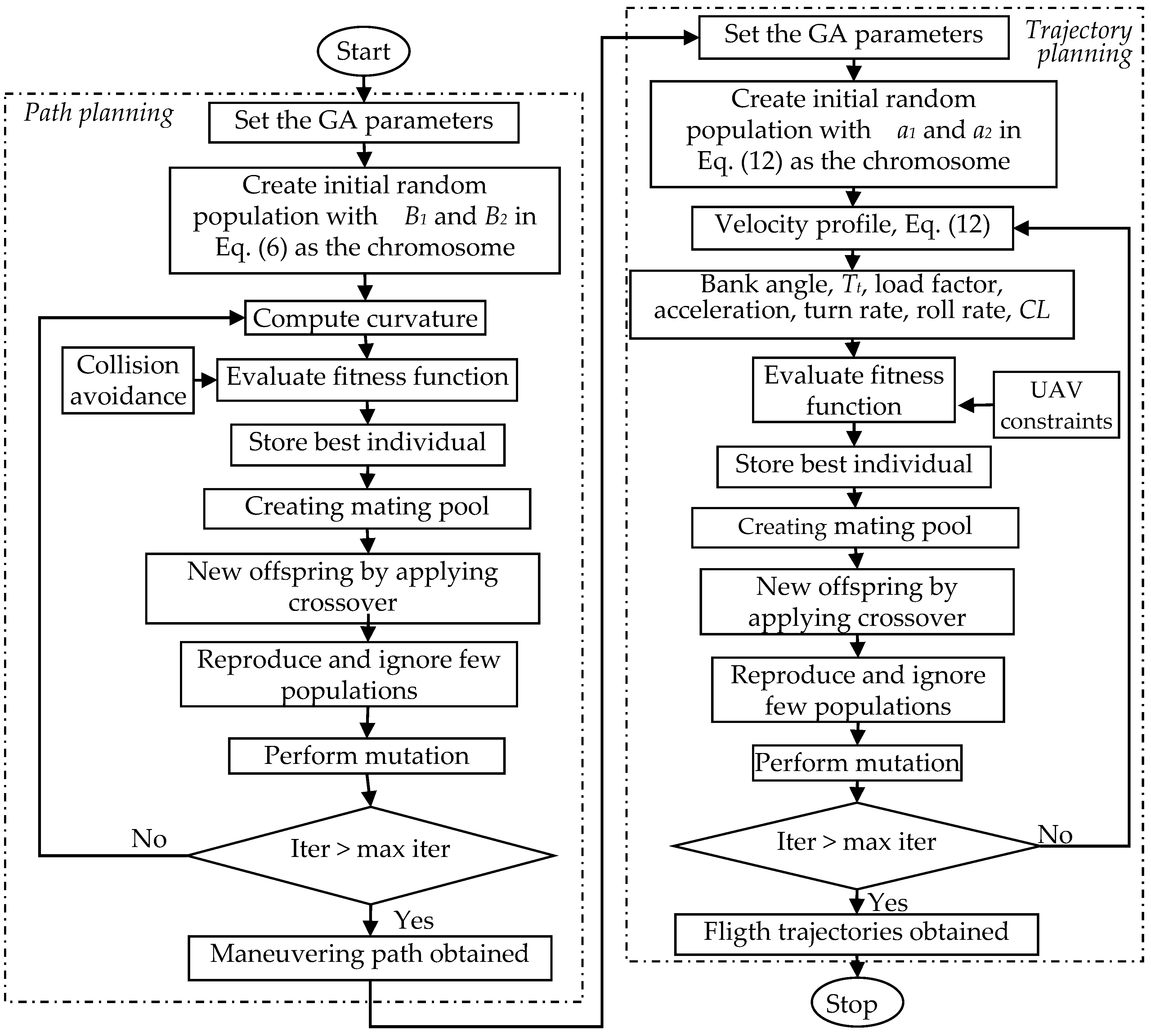
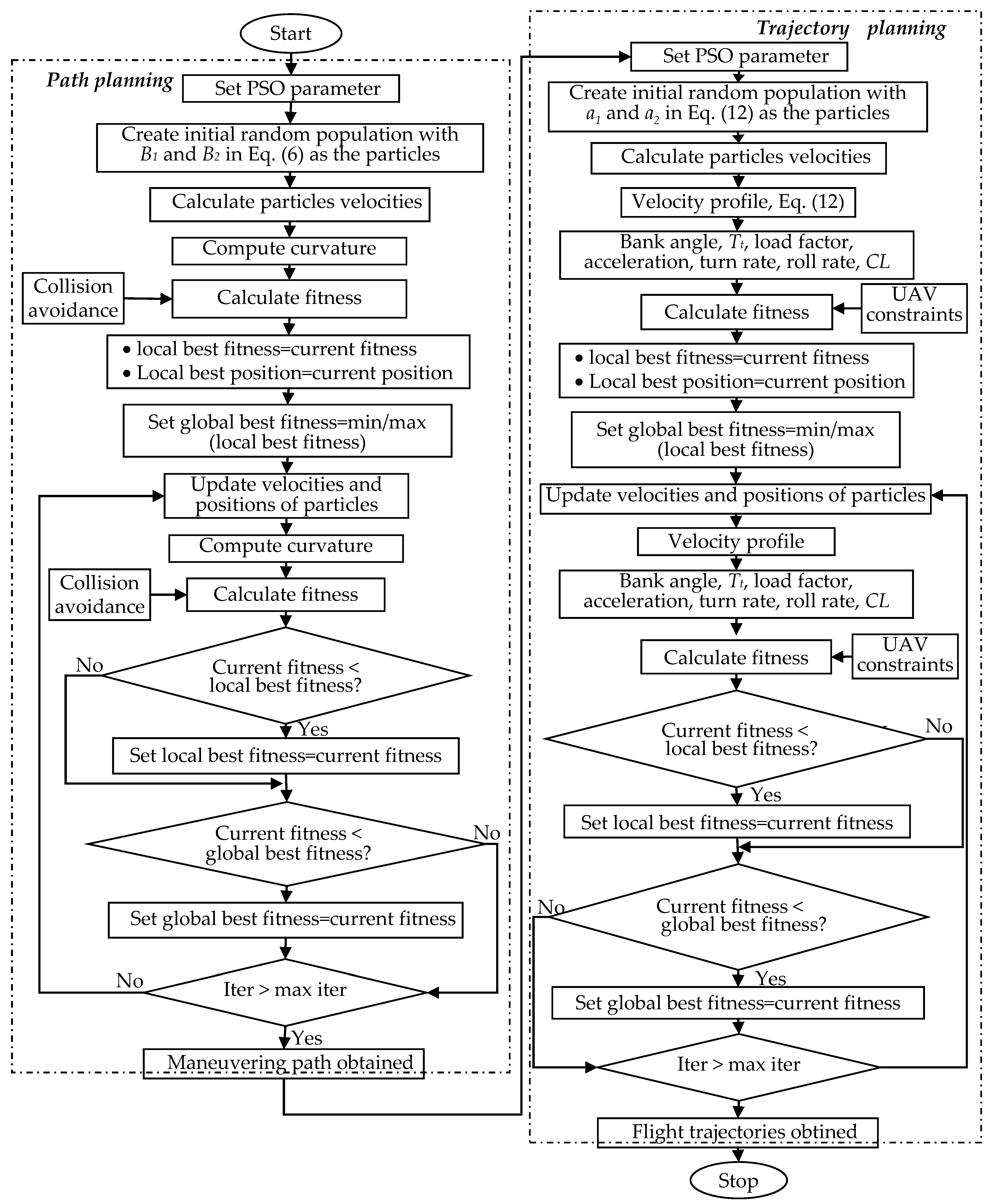
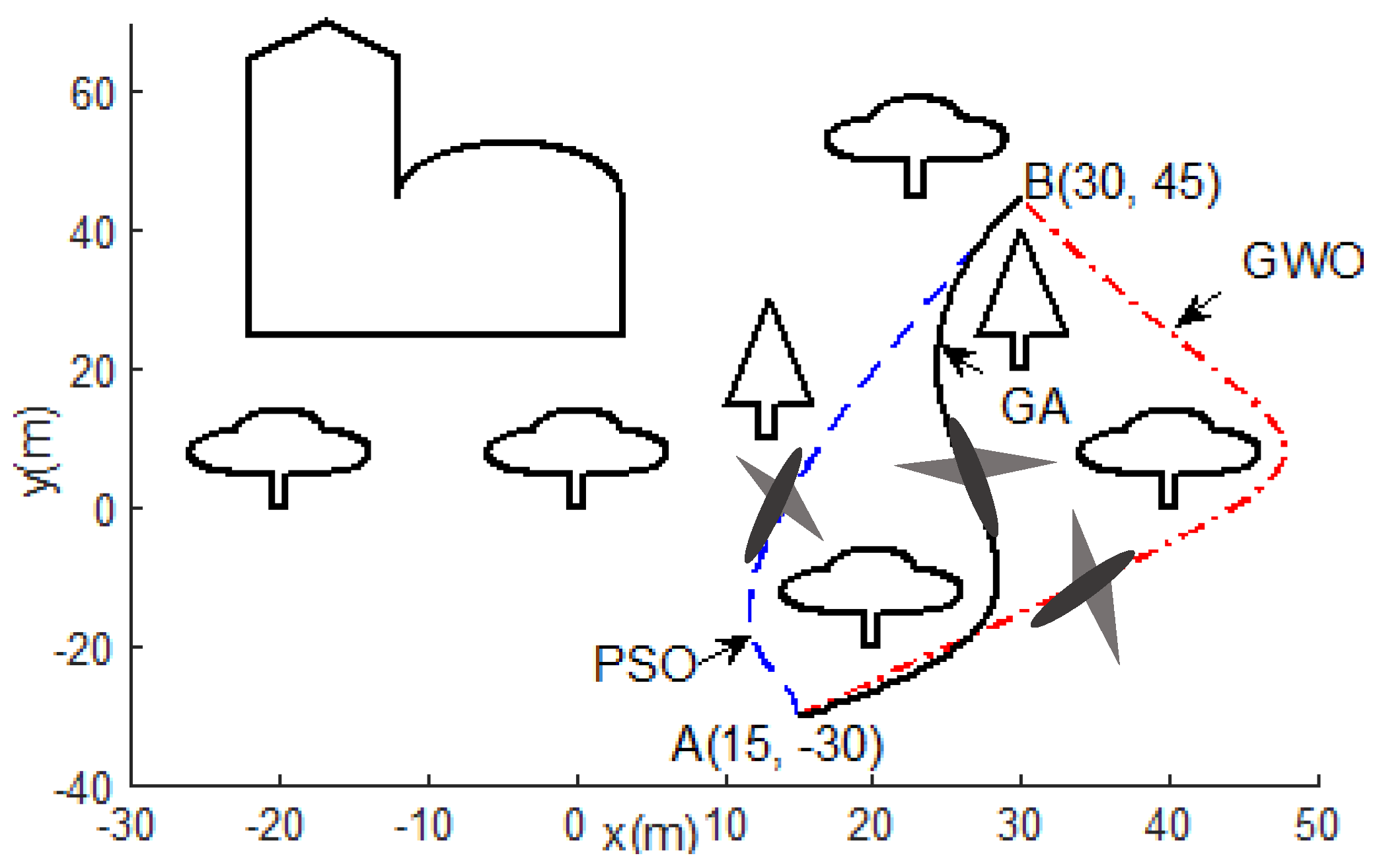
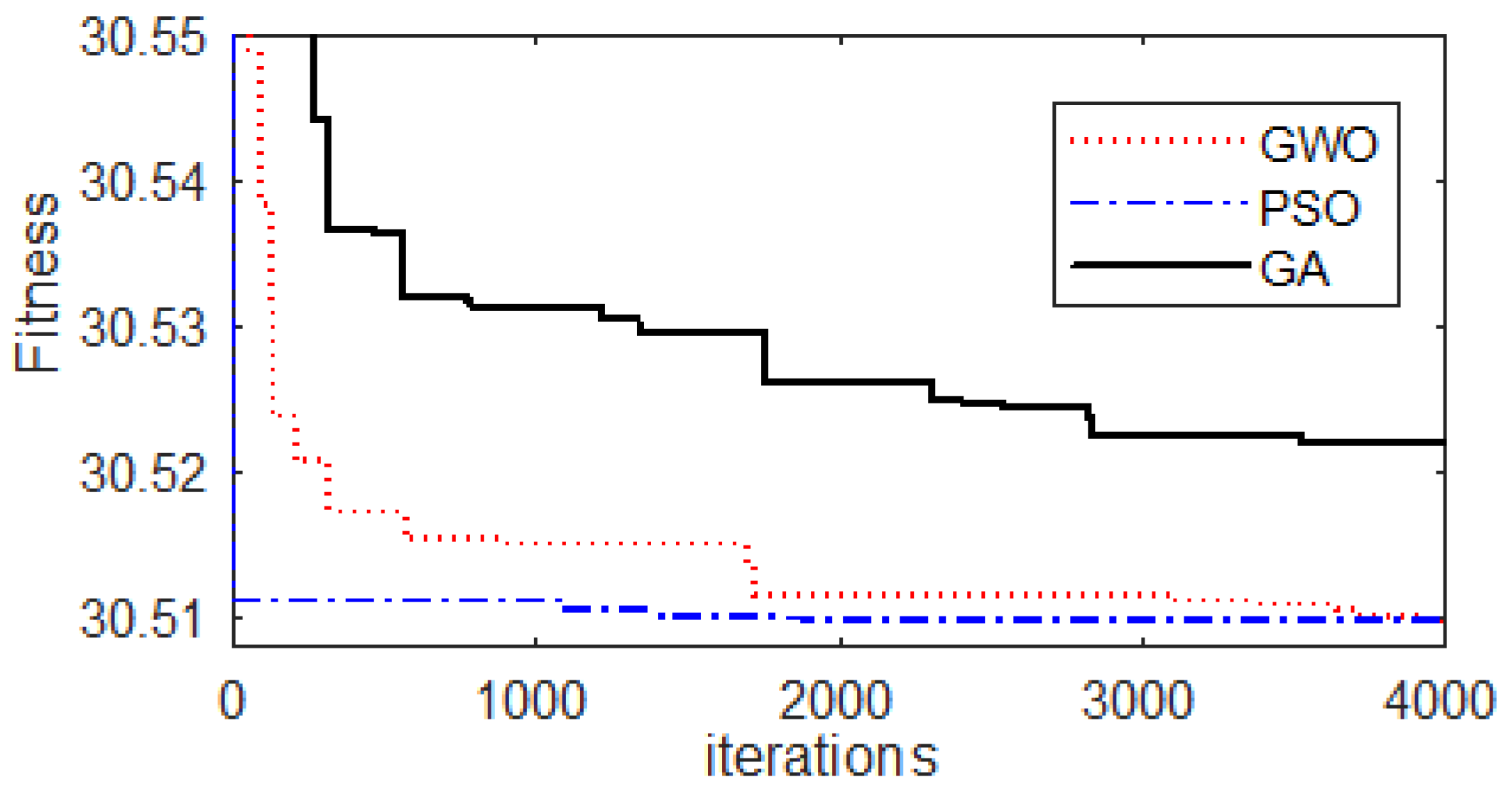
Motivating to improve the maneuvering capability of the conventional fixed-wing UAV, this paper addresses the UAV motion planning using the Bezier curve as the maneuvering path and the variable speed strategy as the flight trajectories generation. The conventional fixed-wing UAV has limitation in performing the bank-turn maneuver. The optimization problem with constraints should be formulated considering all UAV flight performance limitations. 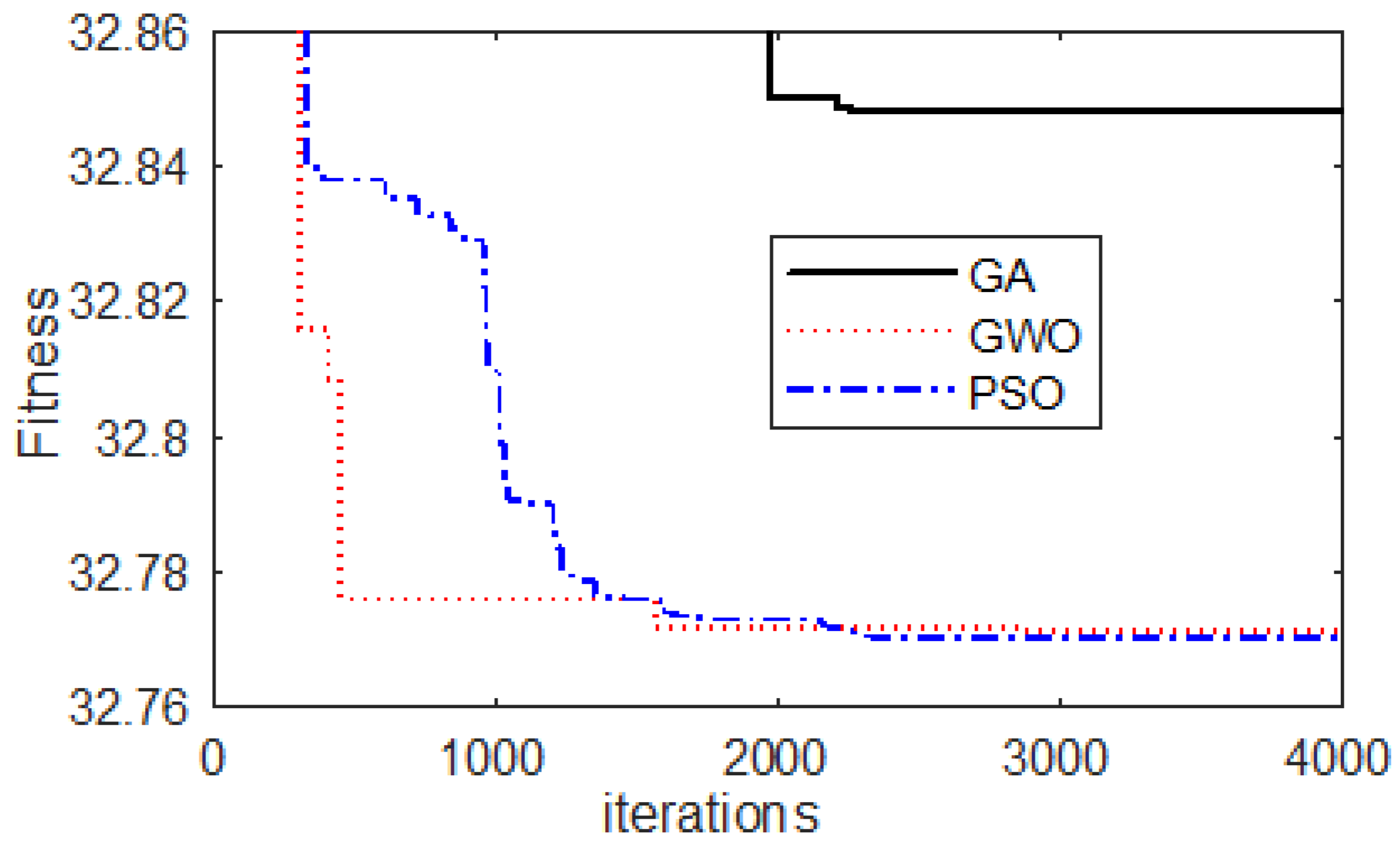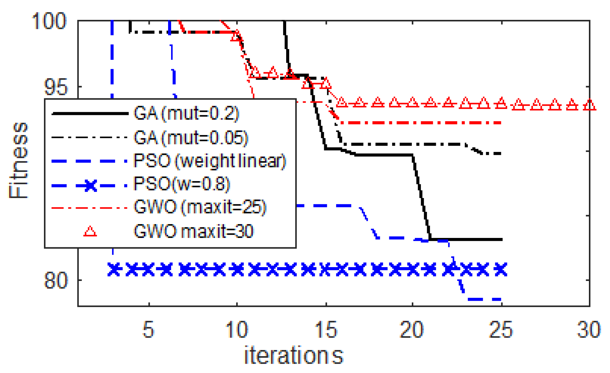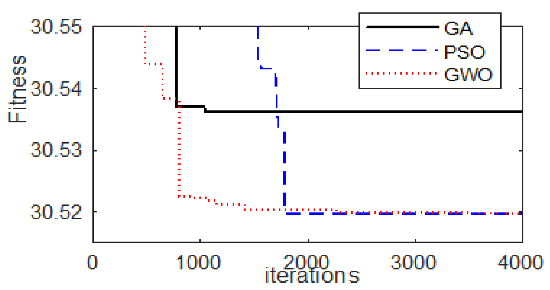In contrast with gradient-based optimizations, the meta-heuristic optimizations do not depend on the derivative of search spaces [23]. Thus, the meta-heuristic optimizations become very promising methods to solve the real engineering problems which has many constraints to be satisfied, as in the case of UAV motion planning problems. The No Free Lunch (NFL) theorem applies to the meta-heuristic optimizations implying that there is no meta-heuristic method best appropriate to solve all optimization problems. A certain meta-heuristic algorithm may show a good performance on a set of optimization problems but having a poor performance on a different set of optimization problems. Thus, for a particular optimization problem, it is necessary to investigate the performance of some meta-heuristic optimizations. In this paper, the performance of three meta-heuristic optimizations, namely the GA, the PSO, and the GWO are investigated in solving the fixed-wing UAV motion planning.

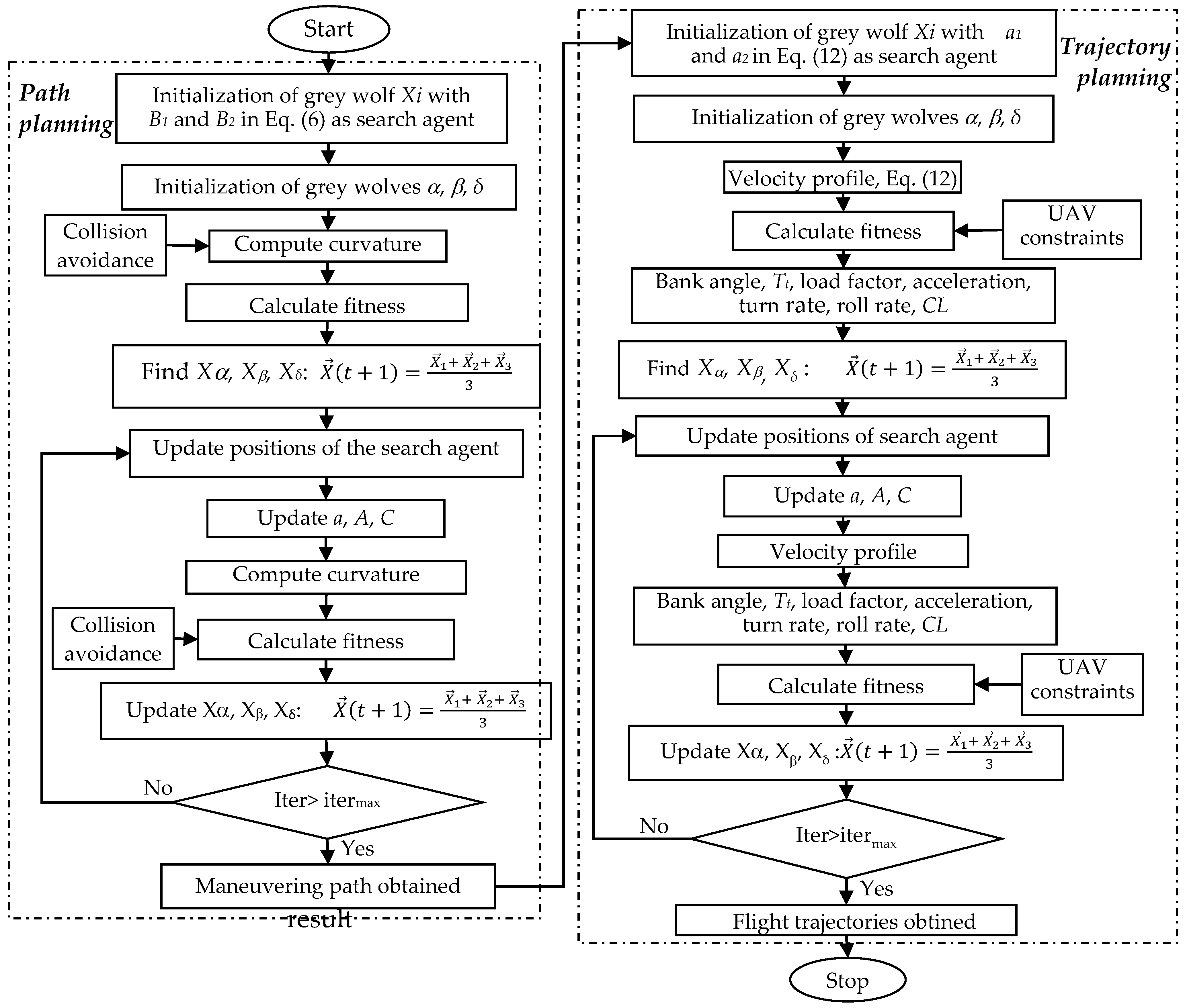
Bezier curve provides the agility and continuity to the flight path. The motion planning is conducted in two steps, which are the path planning and the flight trajectory planning. The path planning objective is to minimize the path length considering the curvature constraint and avoiding collision. Different with typically previous studies, in generating the curvilinear path, this paper does not employ either grid-based technique or RRT algorithm. The Bezier curve is generated directly by searching the optimal Bezier curve control points using meta-heuristic optimizations. The second step is to find the optimal time and load factor considering the flight trajectories constraints. The UAVs perform the Bezier agile path by performing the bank-turn maneuver where the speed and the bank angle, or the roll angle, need to be managed in such a way so that the flight trajectories are optimal and stay in the UAV safe zone. The variable speed is used to perform the bank-turn mechanism. The variable speed plays an important role not only in avoiding the collision with obstacles, but also in preventing an accident and road traffic, and obtaining an optimal time [24].

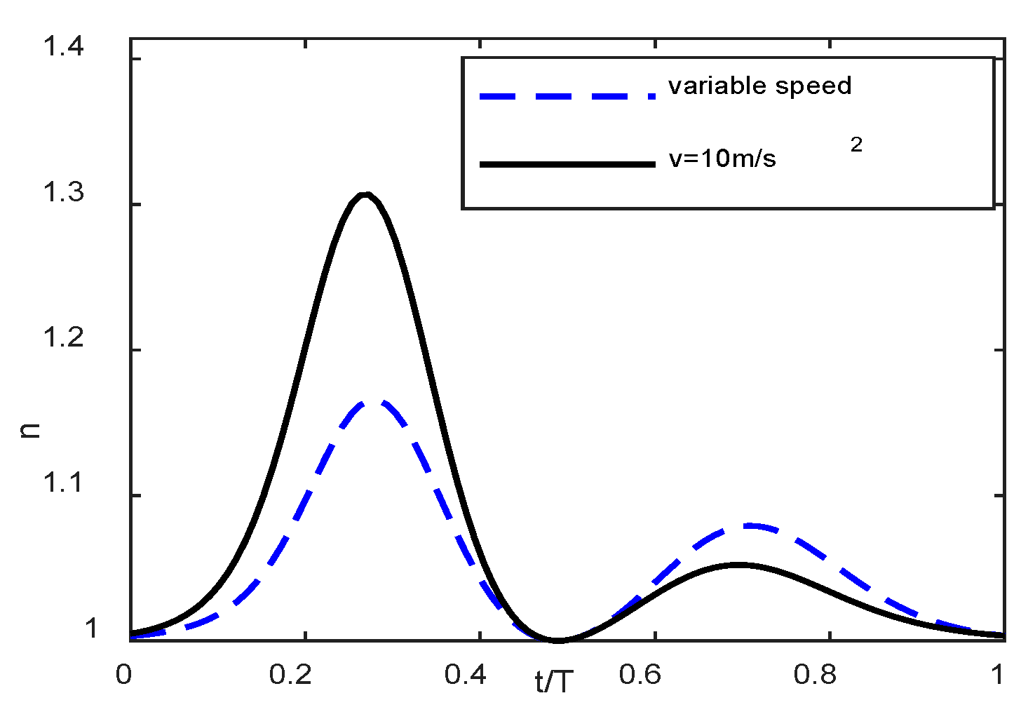
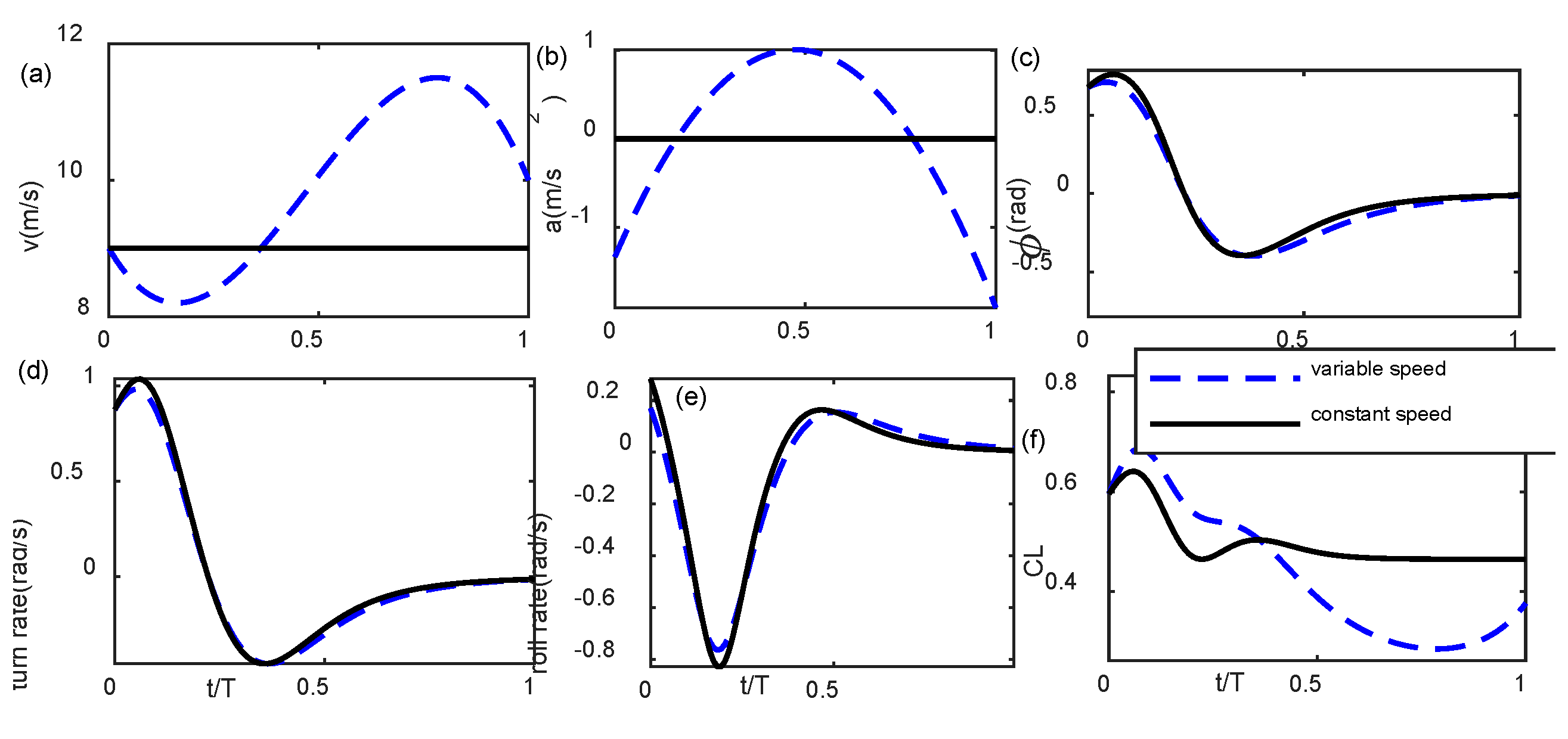
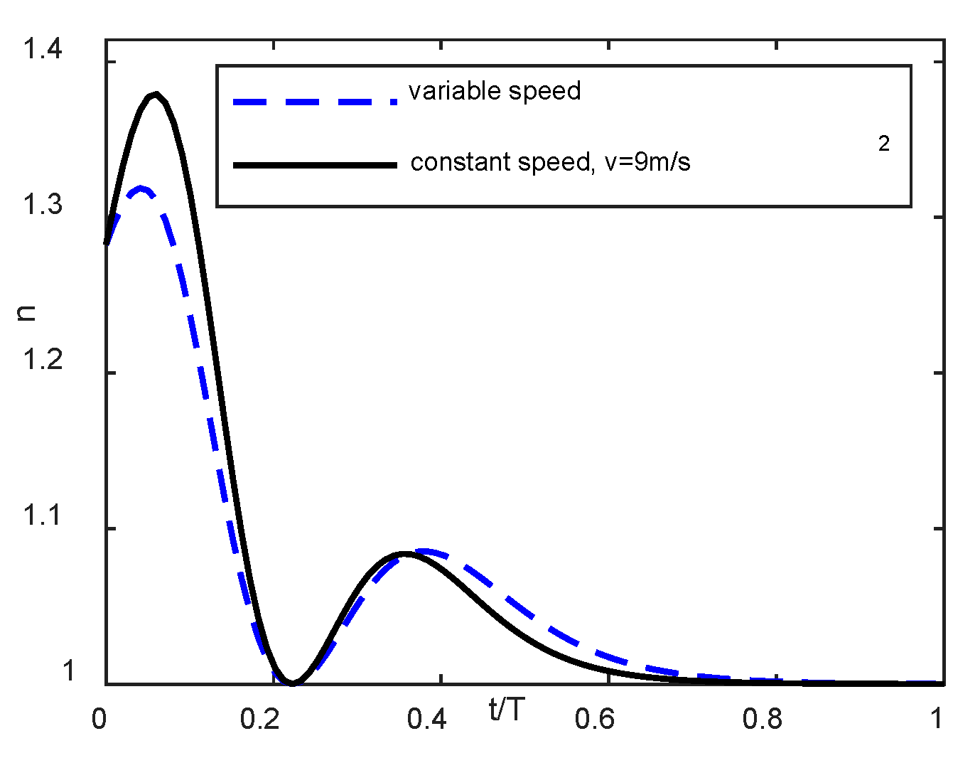
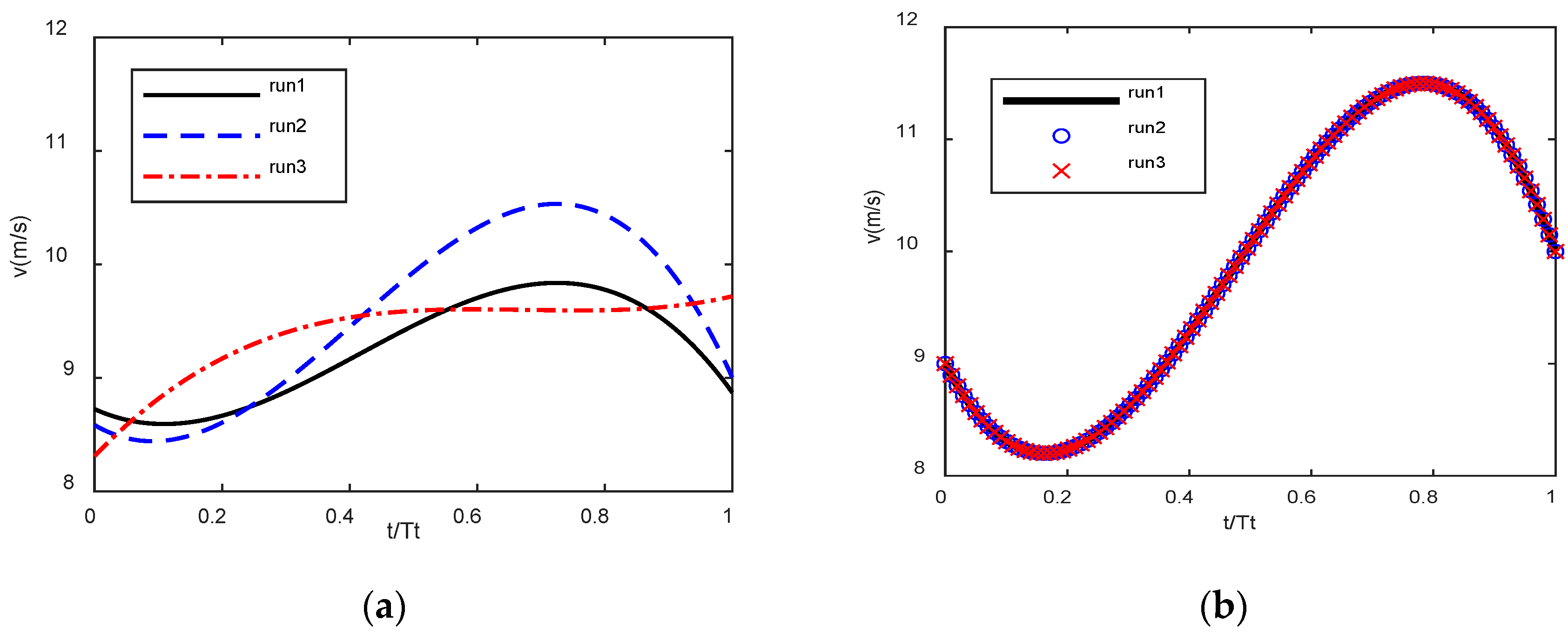
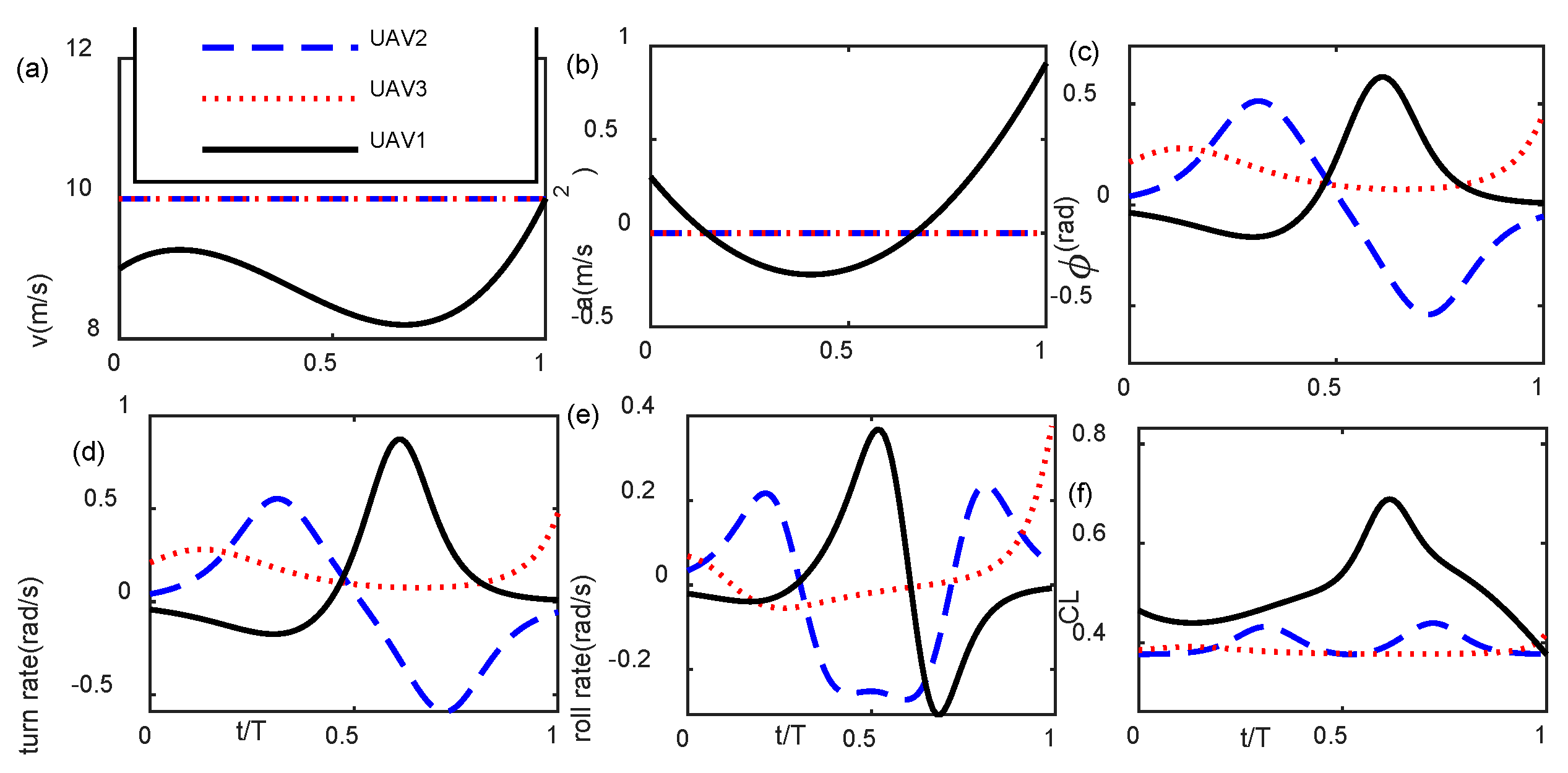
The contributions of this paper are as follows. This paper considers the flight trajectory generation using the variable speed strategy to reduce the load factor distribution during the UAV fixed-wing maneuvering in the normal and tangential coordinate. The load factor distribution plays an important role in the aircraft/UAV maneuvering; however, the load factor behavior during the UAV fixed-wing maneuver is very rarely discussed in studies. 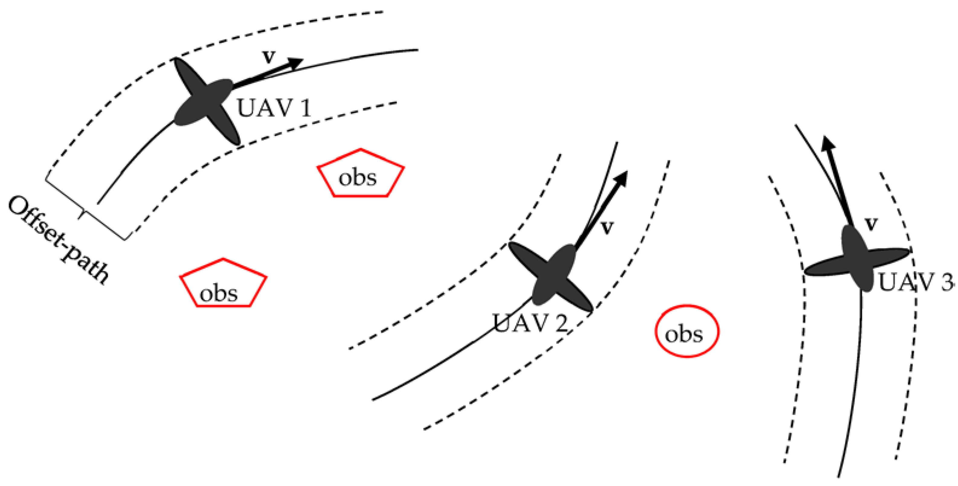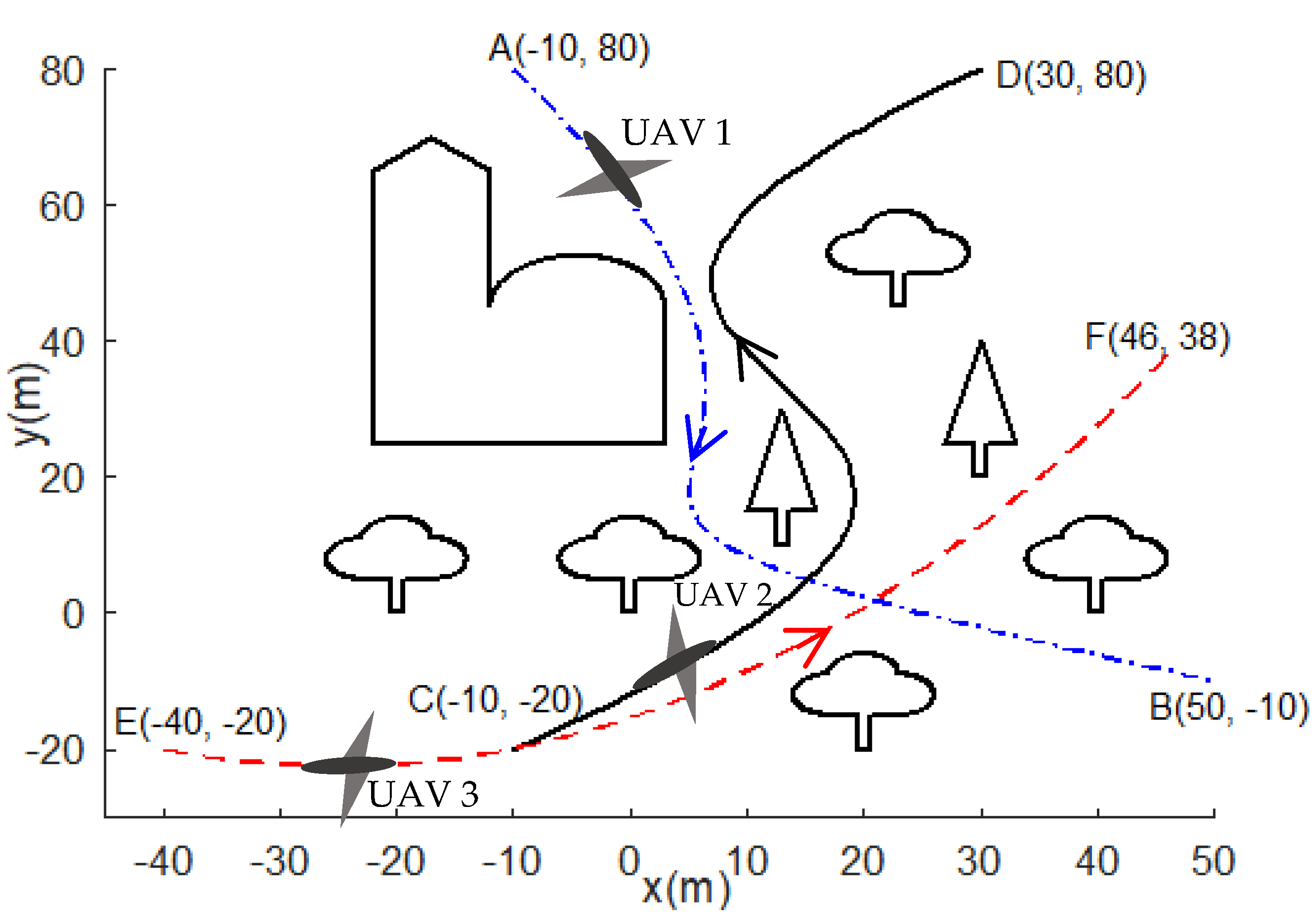An excessive load factor should be avoided because it may indicate a flight operation that exceeds the structural strength [25]. The new computational strategies to generate the speed profile in the normal and tangential coordinate are presented using third-degree polynomials. Instead of only considering the kinematic constraints of the curvature path and collision avoidance, this paper considers the UAV flight constraints, which are the minimum/maximum speed, the minimum/maximum acceleration, the maximum roll angle, and the aerodynamics constraint so the generated trajectories are practically flyable. The trajectory planning is computed based on UAV flight mechanics. Compared with the previous research, the proposed variable speed trajectory generation has only two unknown searching variables. Furthermore, the generated speed trajectories are stable where during different running time, the generated trajectories of the meta-heuristic optimization are convergence. Secondly, the proposed variable speed strategy is applied to the swarm UAVs for simultaneous on target mission. The scenario of the swarm UAV to achieve the simultaneous on target mission using the proposed variable speed strategy is analyzed.

The presentation of the paper is organized as follows. Section 2 presents the material and methods. The proposed path planning and trajectory planning strategies are presented. The variable speed maneuver is developed. Section 3 presents the results and discussions. The single UAV maneuver planning and cooperative UAVs simultaneous on target mission are presented in the numerical simulations. Conclusions of the present paper are presented in Section 4.

2. Materials and Methods

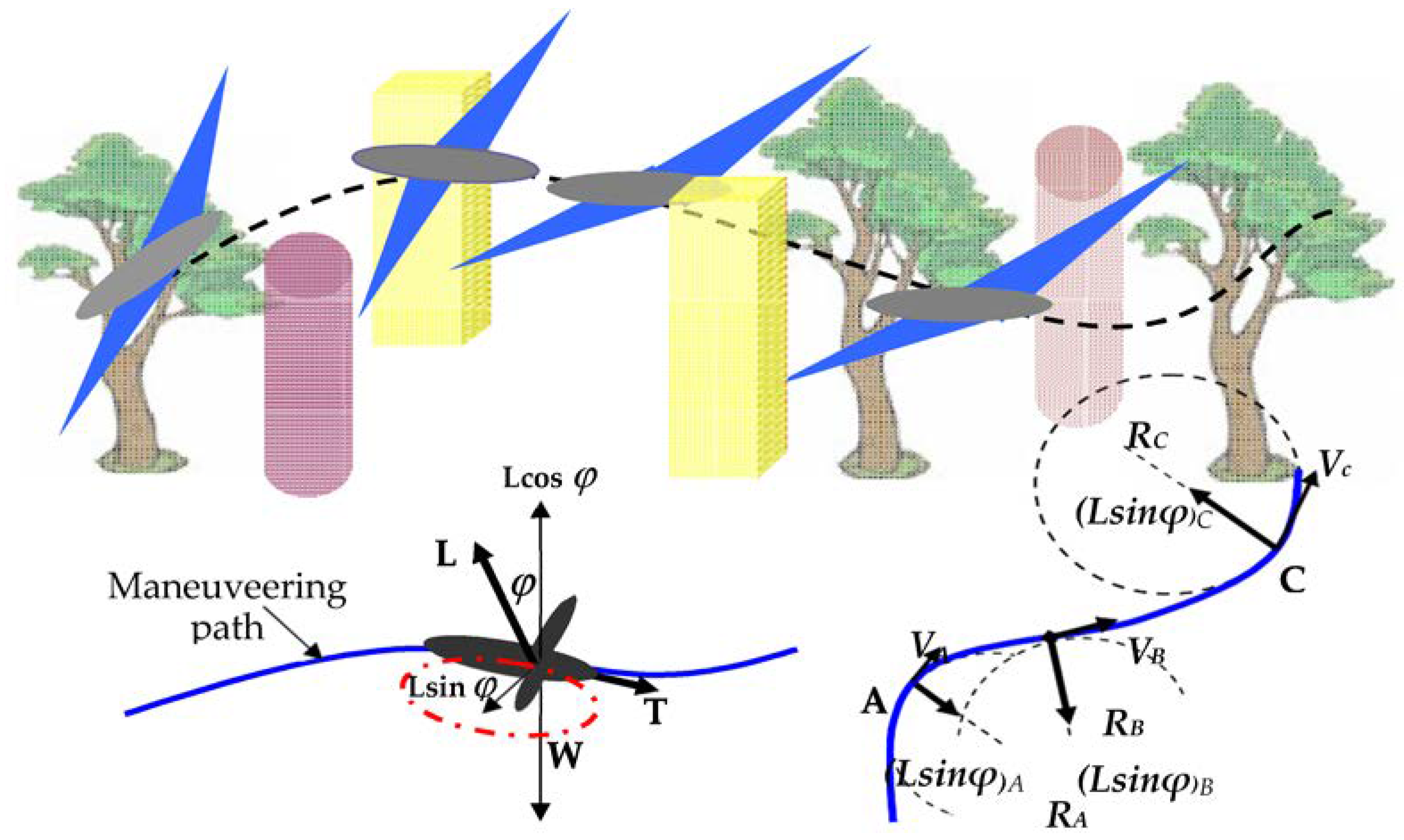
Figure 1 shows the UAV bank-turn maneuver following the curvilinear path. With the curvilinear path using the Bezier curve, the maneuvering path will be adaptable for difficult geometrical environment.

UAV equations of motion of bank-turn mechanism at constant altitude can be expressed as follows [26,27,28]:

$$T-D=ma$$

(1)

$$Lcos \varphi -mg=0$$

(2)

$$Lsin \varphi =m\frac{v^2}{R}$$

(3)

where T, D, m, a, L, $\varphi$, g, v, and R are thrust, drag force, mass, acceleration, lift force, roll angle, gravitational acceleration, velocity, and radius of turn, respectively.

Equations (2) and (3) can be arranged as follows:

$$tan \varphi =\frac{v^2}{R}$$

(4)

By definition, the load factor is expressed as follows:

$$n=\frac{L}{mg}=\frac{1}{cos \varphi }$$

(5)

where n is the load factor.

2.1. Path Planning with Bezier Curve

Originally, the Bezier curve is one of the ab initio design methods developed by Pierre Bezier. Ab initio design is class of shape design problem that depends on both aesthetics and functional requirements. In recent developments, the Bezier curve has been widely utilized in the motion planning of the robot. It has control points which are very agile to be placed as needed in the surveying area.

The Bezier curve is expressed parametrically as follows [18]:

$$\left(\begin{array}{c}x\\ y\end{array}\right)={{\displaystyle \sum }}_{u=0}^n{B}_i J_{n,i}\left(u\right)\hspace{1em}\hspace{1em}0\le u\le 1$$

(6)

$$J_{n,i}\left(u\right)=\left(\begin{array}{c}n\\ i\end{array}\right)u^i{\left(1-u\right)}^{n-i}\hspace{1em}\hspace{1em}\left(\begin{array}{c}n\\ i\end{array}\right)=\frac{n!}{i!\left(n-1\right)!}$$

(7)

where Jn,i(t) is the ith nth order Bernstein basis function, and u is curve parameter. To construct an nth degree Bezier curve, it needs n + 1 control points.

This paper uses the third-degree Bezier curve as the maneuvering path. The UAV has the turning radius limitation. The turning radius relates with the path parameter, namely the curvature. The curvature is very important in the curvilinear motion. The radius of the turn, R, will be equal to K = 1/R. Detail of the curvature constraint is presented in the next section.

The objective optimization of the path planning is the minimum path length. For the parametric curve, the path planning objective can be expressed as follows:

$$S_t=min{{\displaystyle \int }}_0^1\left(\sqrt{{\left(\frac{dx\left(u\right)}{du}\right)}^2+{\left(\frac{dy\left(u\right)}{du}\right)}^2}\right)du$$

(8)

where S_t, x(u) and y(u) are total of the maneuver path length, the equation of Bezier curve in the x-component and y-component at Equation (6).

2.2. Trajectory Planning

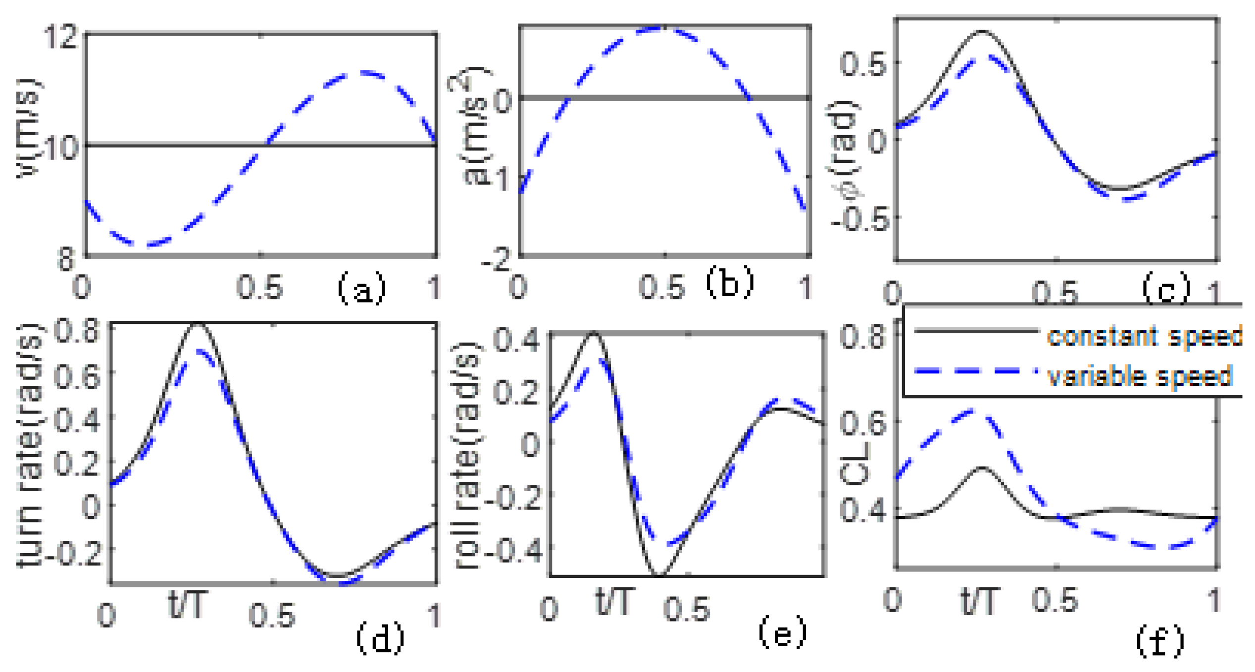
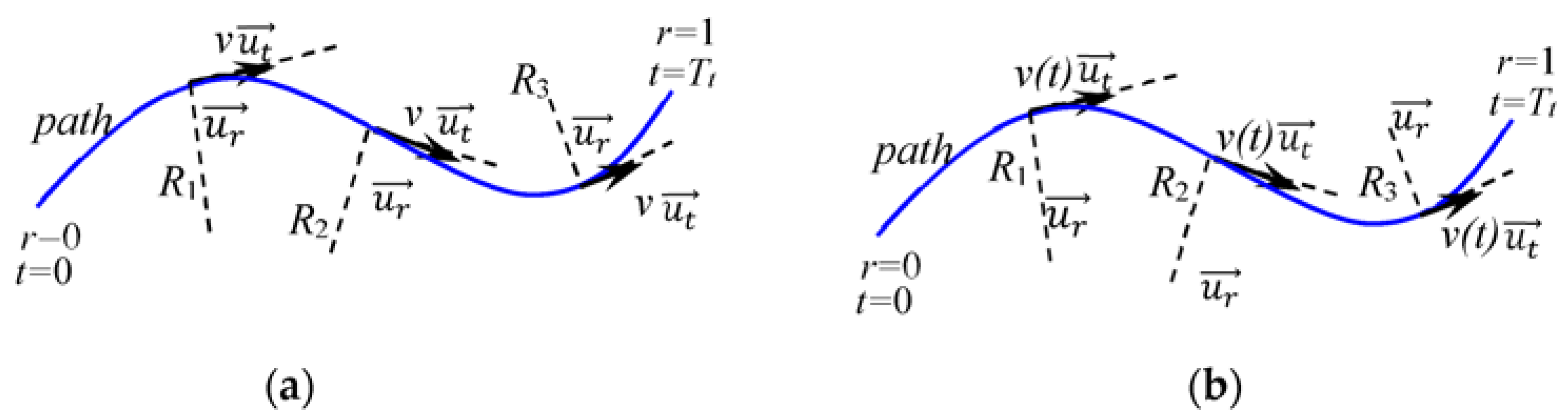
The flight maneuvering can be conducted using either constant speed or variable speed trajectories. This section develops computational strategies to generate the speed profile generation in normal-tangential coordinate. From the path planning, the geometry of the maneuvering curve can be determined, and the heading angle can be computed for the navigation purpose. After the path planning results have been obtained, the trajectory planning analysis in the normal and tangential coordinates is conducted.

Different from the rotor UAV which can hover in the air, the fixed-wing UAV can only move forward; therefore, at the constant altitude, the normal and tangential coordinate can be implemented for analyzing flight maneuvering. Figure 2 illustrates the normal and tangential coordinates for the constant speed and the variable speed. The unit vector $\overrightarrow{u_t}$ with a positive direction is the same as the UAV movement and a unit vector $\overrightarrow{u_r}$ with a positive direction toward the radius center.

Velocity vector is only in tangential component as follows [29]:

$$\overrightarrow{v}=v_t \overrightarrow{u_t}$$

(9)

Acceleration vector consists of tangential and normal components as follows:

$$\begin{gathered} \overrightarrow{a}=a_t\overrightarrow{u_t}+a_r\overrightarrow{u_n} \\ =\frac{dv}{dt}\overrightarrow{u_t}+\frac{v^2}{r}\overrightarrow{u_n} \end{gathered}$$

(10)

2.2.1. Constant Speed

Using the constant speed, the problem is simplified as to choose the constant speed, v, in such a way so that the trajectory optimization objective is achieved. The UAV traveling time can be obtained using the Newton law.

Considering the tangential component, the UAV maneuvering time can be obtained from the tangential component of velocity as follows:

$$T_t=\frac{S_t}{v_t}=\frac{{{\displaystyle \int }}_0^1\left(\sqrt{{\left(\frac{dx\left(u\right)}{du}\right)}^2+{\left(\frac{dy\left(u\right)}{du}\right)}^2}\right)du }{v_t}$$

(11)

The UAV maneuvering speed, v_t, needs to be selected within the UAV speed range: [v_min, v_max]. The total curve length during the maneuvering, S_t, is obtained from the path-planning step.

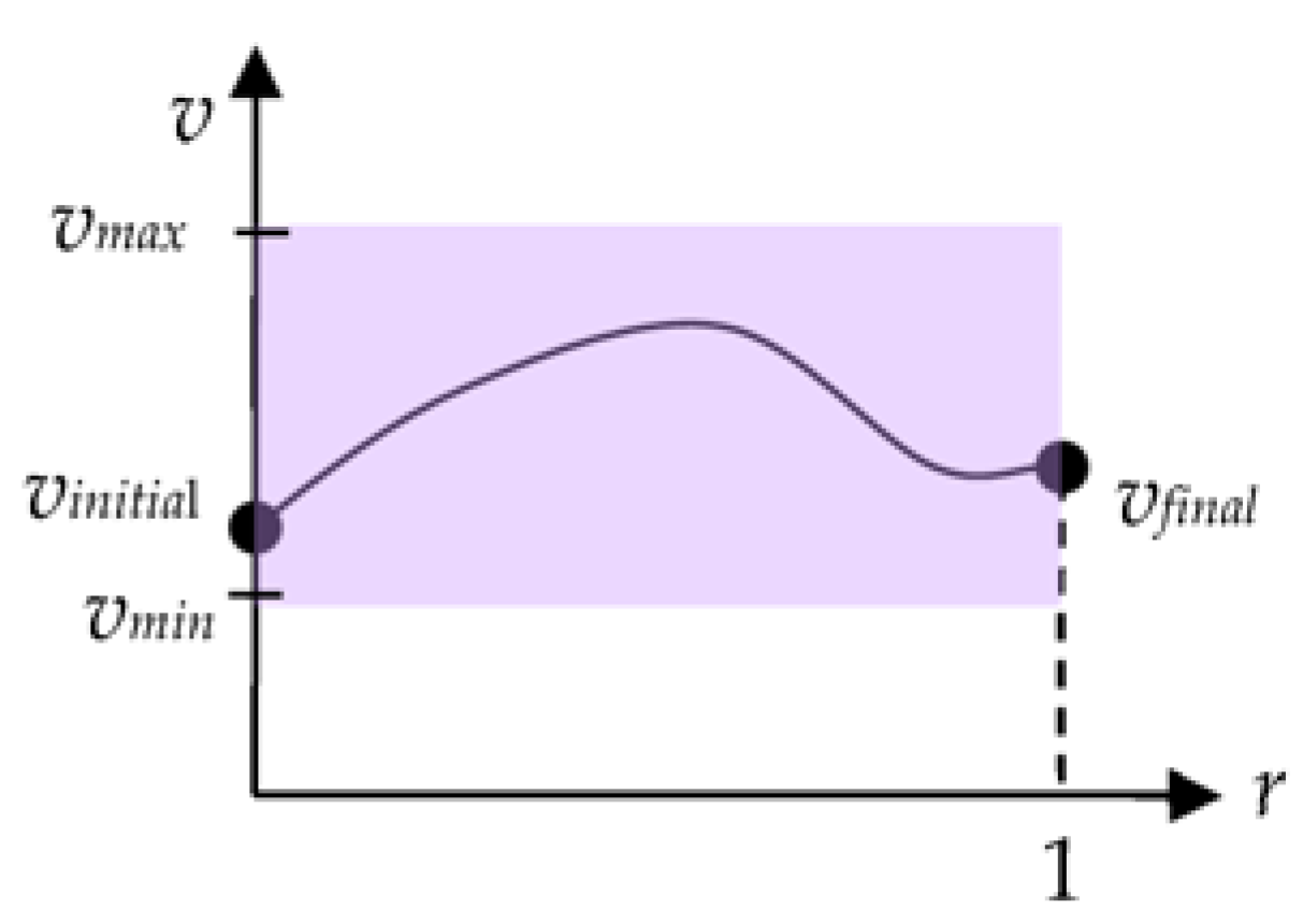
2.2.2. The Variable Speed Strategy

This paper considers the variable speed maneuvering where the speed trajectories profile is generated with the polynomial continuous function. The speed should be managed to stay in the UAV operational area while the flight trajectories are also kept to the optimum. This is a challenging optimization problem since the UAV speed can fall into very low value or very high value which is beyond the UAV operational area.

Figure 3 shows the illustration of this strategy. The initial speed, v_initial, and final speed, v_final, are known and the speed profile should be managed in the UAV allowable speed zone.

This paper uses third-degree polynomial function in generating the speed profile. For third-degree polynomial, the speed equation is in the following

$$v_t\left(t\right)=\left(a_3{r}^3+a_2{r}^2+a_{1}r+a_0\right)\circ r\left(t\right),$$

(12)

where a_n is the nth coefficient of polynomial and r is linear time-scale, $r=\frac{t}{T_t}$, with t is the time variable and T_t is the total maneuvering time.

Substituting the conditions of initial speed and final speed, the following equations of coefficient polynomial can be obtained:

$$a_0=v_t\left(0\right)=v_i$$

(13)

$$a_3=v_f-a_2-a_1-v_i$$

(14)

where v_i is the initial speed at r = 0 and v_f is the final speed at r = 1.

This paper considers known v_i and v_f so that there are two searching parameters, which are a₁ and a₂.

The UAV tangential acceleration is as follows:

$$a_t\left(t\right)=\dot{v_t}\left(r\right)\frac{1}{T_t}$$

(15)

The motion of the UAV can be analyzed using Newton’s law as follows:

$$S_t={{\displaystyle \int }}_0^{T_t}{v}_t\left(t\right)dt$$

(16)

With the linear timescale, $r=\frac{t}{T_t}$, so that $\frac{dr}{dt}=\frac{1}{T_t}$ or $dt=T_t dr$, Equation (16) can be expressed as follows:

$$S_t=\frac{1}{T_t}{{\displaystyle \int }}_0^1{v}_t\left(r\right)dr$$

$$T_t=\frac{S_t}{{{\displaystyle \int }}_0^1{v}_t\left(r\right)dr}$$

(17)

2.3. Constraints

For the planar curve, there is a parameter which is called a curvature, K. Its expression can be written as follows:

$$K=\frac{\dot{x}\ddot{y}-\dot{y }\ddot{x}}{{({\dot{x}}^2+{\dot{y}}^2)}^{\frac{3}{2}}}$$

(18)

where $\dot{x},\dot{y},\ddot{x},$ and $\ddot{y}$ are the first derivative of x, y, and the second derivative of x and y, respectively. Since K = 1/R, the minimum turning radius constraint means the maximum K, K_max.

The curvature constraint can be expressed in the following:

$$-K_{max}\le K\le K_{max}$$

(19)

The speed and acceleration during the flight maneuver should be kept within the operational areas as follows:

$$v_{min}\le v_t\le v_{max}$$

(20)

$$-a_{max}\le a_t\le a_{max}$$

(21)

where v_t, v_min, v_max, a_max, and a_min are the speed, the minimum speed, the maximum speed, the maximum acceleration, and the minimum acceleration, respectively.

The value of a_max can be obtained using Equation (1):

$$a_{max}=\frac{T_{max}-D_{min}}{m}$$

(22)

where a_max, T_max, and D_min are maximum acceleration, maximum thrust, and minimum drag force, respectively.

The minimum drag force can be obtained as follows

$$D_{min}=\frac{1}{2}\rho v_t^{2}S{C}_{d0}$$

(23)

where D_min, $\rho$, v, S, and C_d0 are the minimum drag force, air density, wing surface area, and minimum drag coefficient, respectively.

The UAV has the roll angle limitation which show the flight maneuvering ability as follows:

$$-{\varphi }_{max}\le \varphi \le {\varphi }_{max}$$

(24)

The positive and negative sign in Equation (24) are associated with the curvature value.

The maximum load factor constraint can be obtained from Equations (5) and (24) as follows:

$$n_{max}=\frac{1}{cos{\varphi }_{max}}$$

(25)

This paper considers that UAV flying at positive load factor, thus the constraint of the load factor can be expressed:

$$1\le n\le n_{max}$$

(26)

The UAV has the turn rate constraint as follows:

$$-{\omega }_{max}\le \omega =\frac{gtan \varphi }{v_t}\le {\omega }_{max}$$

(27)

where $\omega$ and ${\omega }_{max}$ are the turn rate and the maximum turn rate, respectively.

The value of maximum turn rate is obtained from:

$${\omega }_{max}=\frac{gtan {\phi }_{max}}{v_{min}}$$

Keeping the flight at constant altitude involves the requirement to manage the lift force. Thus, the coefficient of lift, CL, should be considered also as the constraints in the following:

$$Lcos \varphi =mg$$

(28)

$$\frac{1}{2}\rho v_t^{2}SCL\cos \varphi =mg$$

(29)

$$C{L}_{min}\le CL=\frac{2mg}{\rho v_t^{2}S\cos \varphi }\le C{L}_{max}$$

(30)

where CL, $C{L}_{max}$, $C{L}_{min}$, $\rho$, and S are the lift coefficient, the maximum lift coefficient, the minimum lift coefficient, an air density, and a wing area, respectively. The value of maximum/minimum CL is obtained by substituting the value of maximum/minimum velocity and roll angle in value of CL in Equation (30).

Speed Constraint for Constant Speed Maneuver

Due to the maximum load factor constraint, for the constant speed maneuver, it needs to check the velocity correspond to the minimum radius of the maneuvering path, i.e., $R_{path\_min}$ (see Equation (4)) as follows:

$$v_{max\_}=\sqrt{R_{path\_min}gtan {\varphi }_{max}}$$

(31)

where v_{max_} and $R_{path\_min}$ are maximum velocity corresponds to the maneuvering path and minimum radius of the maneuvering path, respectively.

For the constant speed maneuvering, there is a new range of the feasible constant speed from the minimum speed to the new maximum allowable speed, v_{max_,} as follows:

$$v_{min}\le v_t^2\le v_{max\_}$$

(32)

In the case that v_{max_} > v_max, Equation (20) is applicable.

3. Generating Optimal Flight Paths and Trajectories Using Meta-Heuristic Optimizations

The GA, PSO, and GWO are applied to find the best solution of the path planning and trajectory planning.

3.1. Fitness Function

This section presents the fitness function for the maneuvering planning and the trajectory planning.

3.1.1. Path Planning

The collision detection is performed by checking the UAV positions during the flight maneuvering whether they are inside the obstacle area or intersect with other UAVs as the dynamic obstacles. During the flight, the off-set path is applied for safety due to UAV has the wingspan. Figure 4 illustrates the environment during the UAV maneuvering at constant altitude. For the single UAV, the static obstacles are applied while for the cooperative UAVs, besides the static obstacles, other UAVs become the dynamic obstacles.

Fitness function of the path planning for meta-heuristic optimization is expressed as follows:

$$Fitness{\displaystyle \{}\begin{array}{cc}=C& \exists \left\{K \langle -K_{max}or K\rangle K_{max} or \left(x,y\right){{\displaystyle \cap }}^{ }obstacle area or \left(x,y\right){{\displaystyle \cap }}^{} {\left(\mathrm{UAV}\right)}_{obs}\right\}\hfill \\ =S_t& else\hfill \end{array}$$

(33)

where C, (x, y), L, ${\left(\mathrm{UAV}\right)}_{obs}$ are constant value, UAV positions, length and other UAVs as dynamic obstacle.

3.1.2. Trajectory Planning

Since the curvilinear motion involves continuously change the turning radius so that the bank angles or roll angles are varied, the load factors are also varied during the maneuver. It is very important to perform the maneuver in the allowable load factor to avoid a structural damage [25]. Thus, the objective of optimization is to minimize the time and load factor.

Fitness function of the flight trajectory planning is expressed as follows:

$$Fitness\{\begin{array}{cc}=C& \exists \left\{\begin{array}{c}{v}_{min}\le v\le v_{max} or -a_{max}\le a\le a_{max} or -{\varphi }_{max}\le \varphi \le {\varphi }_{max} or\hfill \\ -{\omega }_{max}\le \omega \le {\omega }_{max} or C{L}_{min}\le CL\le C{L}_{max} or T>T_{target} or n>n_{target}\hfill \end{array}\right\}\\ =F_2& else\hfill \end{array}$$

(34)

$$F_2=aT+\left(1-a\right) 0.5 {{\displaystyle \sum }}_{i=1}^{i=k}n$$

(35)

where $T_{target}$, $n_{target}$, a and 0.5 are the target of maneuvering time, target of load factor, weighting factor and normalized factor, respectively.

Both path planning and trajectory planning apply the penalty method in the fitness function. To achieve the advantage of the variable speed strategy over the constant speed strategy, the target of maneuvering time, $T_{target}$, and the target of load factor, n_target, are considered in the fitness function.

3.2. Genetic Algorithm

Mainly, there are three operators in the GA: reproduction, crossover, and mutation. The optimization parameter is converted to the chromosomes and coded it in the evolution process. Using the real code GA, the chromosome is represented as the number in sequence. The selection is the process to choose two individuals in the population as parents for mating to form the new offspring. A crossover is a process of randomly picking one or more individuals as parents and swapping segments of the parents. This paper uses random resetting mutation. In this scheme, a randomly chosen gene is assigned to be changed with a random value. The detailed procedure of the GA can be referred to [30]. Figure 5 illustrates the flowchart of the GA to solve the fixed-wing UAV motion planning.

3.3. Particle Swarm Optimization

PSO was firstly proposed by Kennedy and Eberhart, inspired by the social behavior of animals, such as birds flocking or fish schooling [31]. The optimization variables are represented as particles which move with certain velocity value. Figure 6 illustrates the flowchart of the PSO to solve the fixed-wing UAV motion planning.

Velocities and positions are updated based on the local and global best solutions:

$$v_{t+1}=v_t+{\phi }_1{\beta }_1\left(p_i-x_i\right)+{\phi }_2{\beta }_2\left(p_g-x_i\right)$$

(36)

$$x_{t+1}=x_i+v_{t+1}$$

(37)

where v_t, v_t+1, φ₁, and φ₂ are the velocity, the update velocity, cognitive parameter, social parameter, respectively.${\beta }_1$ and ${\beta }_2$ are independent uniform random numbers, p_i and p_g are best local solution, and best global solution, whereas x_i is the current position of each particle.

Shi and Eberhart [32] introduced an inertia weight factor, w, to the velocities as follows:

$$v_{t+1}=w{v}_t+{\phi }_1{\beta }_1\left(p_i-x_i\right)+{\phi }_2{\beta }_2\left(p_g-x_i\right)$$

(38)

Eberhart and Shi [33] improved the velocity by utilizing the constriction factor, $\chi$, in the following:

$$v_{t+1}=\chi \left\{w{v}_t+{\phi }_1{\beta }_1\left(p_i-x_i\right)+{\phi }_2{\beta }_2\left(p_g-x_i\right)\right\}$$

(39)

$$\chi =\frac{2}{2-\phi -\sqrt{{\phi }^2-4\phi }}; \phi ={\phi }_1+{\phi }_2,\phi >4$$

The weighting factor, w, can be in form of constant, linear, random, chaotic, and others. This paper uses the linear weighting factor as follows:

$$w=\frac{N_{max}-iter}{N_{ma}{}_x}$$

(40)

where N_max and iter are a maximum iteration number and a current iteration, respectively.

3.4. Grey Wolf Optimization

The GWO is the meta-heuristic optimization developed by Mirjalili et al. [23] in 2014. It is inspired from hunting mechanism and leadership hierarchy of grey wolves. The GWO has four types of grey wolves, namely alpha (α), beta (β), delta (δ), and omega (ω).

The fittest, second, and third best solutions correspond to alpha (α), the beta (β), and delta (δ), respectively. The omega (ω) wolves are other candidate solutions which follow α, β, and δ during the hunting mechanism.

Grey wolves can identify the location of prey. The alpha is guided the hunt process. In the GWO, the first three best solutions are saved, and the other search agents are updated their positions based on the position of the best search agents.

The following formulas are applied to simulate the hunting mechanism:

$${\overrightarrow{D}}_{\alpha }=\left|{\overrightarrow{C}}_1\cdot {\overrightarrow{X}}_{\alpha }-\overrightarrow{X}\right|; {\overrightarrow{D}}_{\beta }=\left|{\overrightarrow{C}}_2\cdot {\overrightarrow{X}}_{\beta }-\overrightarrow{X}\right|; {\overrightarrow{D}}_{\delta }=\left|{\overrightarrow{C}}_3\cdot {\overrightarrow{X}}_{\delta }-\overrightarrow{X}\right|$$

$${\overrightarrow{X}}_1={\overrightarrow{X}}_{\alpha }-{\overrightarrow{A}}_1\cdot \left({\overrightarrow{D}}_{\alpha }\right); {\overrightarrow{X}}_2={\overrightarrow{X}}_{\beta }-{\overrightarrow{A}}_2\cdot \left({\overrightarrow{D}}_{\beta }\right); {\overrightarrow{X}}_1={\overrightarrow{X}}_{\alpha }-{\overrightarrow{A}}_1\cdot \left({\overrightarrow{D}}_{\alpha }\right)$$

(41)

$$\overrightarrow{X}\left(t+1\right)=\frac{ {\overrightarrow{X}}_1+{\overrightarrow{X}}_2+{\overrightarrow{X}}_3}{3}$$

where t, $\overrightarrow{A}$, $\overrightarrow{C}$, ${\overrightarrow{X}}_p$, $\overrightarrow{X}$ are the current iteration, coefficient vector, coefficient vectors the position vector of the prey, and the position vector of a grey wolf, respectively.

Vectors $\overrightarrow{A}$ and $\overrightarrow{C}$ are expressed as follows:

$$\begin{gathered} \overrightarrow{A}=2\overrightarrow{a}·{\overrightarrow{r}}_1-\overrightarrow{a} \\ \overrightarrow{C}=2·{\overrightarrow{r}}_2 \end{gathered}$$

(42)

where $\overrightarrow{a}$ are linearly decreased from 2 to 0 during the iterations. ${\overrightarrow{r}}_1$ and ${\overrightarrow{r}}_2$ are random vectors in the range [0, 1].

Figure 7 illustrates the flowchart of the GWO to solve the fixed-wing UAV motion planning.

4. Results and Discussions

All computations of the path planning and the trajectory planning are performed by writing the computer code in MATLAB environment. The GA, PSO, and GWO use 20 individuals in the population. The optimization parameters are searched within the search area [−100, 100]. The simulations use Ascent UAV which has flight characteristic as shown in

Table 1. Ascent UAV flight characteristics [21,34].

Ascent UAV Flight Characteristics
Mass: 0.553 kg Wing surface are: 0.2135 m2 Wingspan: 1.37 m Minimum Drag coefficient (Cd0: 0.003)	v: (8 ms, 12 ms) $\varphi$: (−π/4, π/4) rad T: (0, 3.7975) N

[11]. These values of constraints are substituted into the equations of constraints. The UAVs fly at the low constant altitude where at that altitude, the air density, ρ, is 1.35 kg/m³. This paper uses 500 as the penalty or C values in Equations (33) and (34) and 0.5 as the weighting factor in Equation (35). For the speed constraint for the safety factor, the value of speed range in the computation is arranged as v_min+δ1 ≤ v ≤ v_max−δ2 with the detail value: 8.2 ≤ v ≤ 11.5. The same arrangement is implemented for the curvature constraint where the factor δ is applied.

4.1. Single UAV

The UAV performs the maneuvering from point A(15, −30) to point B(30, 45) at constant altitude in the obstacle environment. The path is the cubic Bezier curve which has four control points. Point A is the first control point, and point B becomes the fourth control point. The second and third control points are optimized using meta-heuristic optimizations to find the minimum path length under the minimum turning radius and collision avoidance constraints.

4.1.1. Maneuvering Path

This section investigates the performance of the GA, PSO, and GWO to solve the UAV path planning. For the GA, this paper uses a selection rate of 0.5. For the PSO, the cognitive parameter, social parameter, and constriction factor are 1.5, 1.5, and 1, respectively. Effect of parameter selection is observed. For the GA, effect of mutation rate is investigated. The high mutation rate, which has a value of 0.2, and the low mutation rate, which has a value of 0.05, are selected. For the PSO, effect of the weight factor, w in Equation (39), is investigated. The linearly weight factor, Equation (40), and constant weight factor, which has a value of 0.8, are compared. For the GWO, the parameter a, in Equation (42), depends on the value of the maximum iteration number, N_max. Thus, the effect of N_max is investigated. Two values of the maximum iteration numbers, which are N_max = 25 and N_max = 30, are compared.

Table 2. Maneuvering path results.

		GA		PSO		GWO
		Mut = 0.2	Mut = 0.05	$\mathit{w}=\frac{{\mathit{N}}_{\mathit{m}\mathit{a}\mathit{x}}-\mathit{i}\mathit{t}\mathit{e}\mathit{r}}{{\mathit{N}}_{\mathit{m}\mathit{a}\mathit{x}}{}_{}}$	w = 0.8	Nmax = 25	Nmax = 20
Fitness (m)		83.0259	89.7376	78.4397	80.8277	92.142	93.4574
Bezier Control points (m)	B1x	49.3549	64.206	15.6493	3.7845	62.292	33.3489
	B1y	−1.9906	−9.93303	−20.0975	−14.1863	16.955	−7.6005
	B2x	0.9950	−0.163847	0.9754	4.8176	50.194	70.1638
	B2y	−4.2271	24.8555	−24.2947	−19.1839	−0.82175	−0.7684
vmax_ (m/s)		10.903	11.803	9.2336	80.8277	9.4689	10.9416

presents the results of the GA, PSO, and GWO. According to the fitness value results, it shows that the GA with the high mutation rate, i.e., 0.2, has better performance than that of the GA with the low mutation rate, i.e., 0.05. The path planning contains the collision avoidance problem which is a challenging computational problem. The high mutation rate can be used to further explore the searching space and avoid local optima [35,36]. This advantage of the high mutation rate has been observed in the collision avoidance problem of the UAV path planning.

The PSO with linearly weighting factor shows better performance than that of the PSO with the constant weighting factor, i.e., 0.8. The GWO with 25 iteration numbers has better performance than that of the GWO with 30 iterations numbers. Figure 8 illustrates the fitness value for the GA, PSO, and GWO for those different parameter value. It shows that during 25 iterations, the PSO with linearly weighting factor has lowest fitness value than the GA and GWO. The GA yields better fitness value than that of the GWO. Figure 9 shows the maneuvering paths obtained from the GA with 0.2 as mutation rate, PSO with linearly weighting factor, and GWO with 25 iteration numbers. The paths obtained from the GA, PSO, and GWO have different routes and they are collision-free. It can be observed that the path obtained from the PSO employing the linear weighting factor has shortest length compared with the other paths.

These results of the best parameter values of the GA, the PSO, and the GWO are used as the guidance for the selection of the parameter values of each meta-heuristic optimization, for next simulations. Thus, for all presentation of the next sub sections, the GA mutation rate of 0.2 is selected and the linearly weighting factor is used for the PSO. For the GWO, the 25-iteration number is selected in the UAV path-planning case.

4.1.2. Flight Trajectories

The maneuvering path has been obtained. Since the PSO yields the lowest path length, in this section, the flight trajectories obtained by the PSO are optimized using the meta-heuristic optimizations for the variable speed strategy.

Table 3. Variable speed results of PSO maneuvering path.

	GA	PSO	GWO
Fitness	30.5219	30.5097	30.5098
(a2, a1)	(38.0279, −10.0389)	(39.27, −10.5721)	(39.2579, −10.5707)
Time (s)	7.9158	7.9397	7.9402
nmax	1.3214	1.3189	1.3189

shows the results of the fitness value of the variable speed strategy using the GA, PSO, and GWO. It can be observed that the PSO has outperform other meta-heuristic methods. In the trajectory planning, the GWO yields better fitness value than that of the GA. The GWO fitness value has very small different with the PSO results. The speed trajectories of the variable speed strategy should be selected within the speed range, i.e., 8 m/s ≤ v ≤ 12 m/s (Table 1). It shows that the PSO has lowest fitness value than the GA and GWO. Figure 10 illustrates the fitness value evolution of the GA, PSO, and GWO during 4000 iterations. Figure 11 shows the flight trajectories of the variable speed obtained from the PSO, which yields the lowest fitness value, compared with the constant speed maneuver. As can be seen from Table 1, the PSO path has v_{max_} = 9.2336 m/s, thus if the constant speed is performed, the speed should be selected within 8 m/s ≤ v ≤ 9.2336 m/s. This paper chooses v = 9 m/s as the constant speed strategy. The speed profile and acceleration trajectories are shown in Figure 11a,b, respectively. The generated speeds are within UAV allowable zone, i.e., 8 m/s ≤ v ≤ 12 m/s. The roll angle, turn rate, and roll rate trajectories of the variable speed do not show much different with the constant speed trajectories as shown in Figure 11c–e, respectively. The CL trajectories of the constant speed show quite different with the CL trajectories obtained from the variable speed, as shown in Figure 11f. All of these flight trajectories are inside their allowable zone.

Figure 12 shows the load factor distributions of the constant speed strategy compared with the load factor distribution of the variable speed maneuver. It shows that the variable speed has succeeded in reducing the load factor trajectories. The $T_{target}$ and $n_{target}$ in Equation (34) used are 9 s and 1.33, respectively. The maneuvering time using the speed profile obtained from the PSO is completed in 7.9402 s, as can be seen in Table 3.

4.1.3. Path from the GA

The maneuvering path obtained from the GA, PSO, and GWO has different route paths. Since the monitoring flight route of the UAV can be in many possible ways, the path obtained from the GA (see Table 1) is evaluated in this section.

Table 4. Variable speed results (using path from GA).

	GA	PSO	GWO
Fitness	30.5362	30.5194	30.5197
(a2, a1)	(33.9319, −9.22891)	(36.967, −10.2483)	(36.959, −10.24)
Time (s)	8.4977	8.4993	8.4981
nmax	1.1721	1.1654	1.1655

shows the results of the fitness value of the variable speed strategy using the GA, PSO, and GWO of the GA path. It shows that the PSO has lowest fitness value than the GA and GWO. The GWO yields better fitness value than that of the GA. The GWO yields better fitness value than that of the GA. The GWO fitness value has very small different with the PSO results. Figure 13 shows the fitness value evolution of the GA, PSO, and GWO during 4000 iterations. Figure 14 shows the flight trajectories of the variable speed obtained from the PSO compared with the constant speed maneuver.

As can be seen from Table 1, the PSO path has v_{max_} = 10.903 m/s, thus the constant speed chooses v = 10 m/s as the speed maneuver. The speed profile and acceleration trajectories are shown in Figure 14a,b, respectively. The same as in the PSO path, the roll angle, turn rate, and roll rate trajectories of the variable speed and the constant speed do not show much different as shown in Figure 14c–e, respectively. The CL trajectories of the constant speed show quite different with CL trajectories obtained from the variable speed, as shown in Figure 14f.

Figure 15 shows the load factor distributions of the constant speed strategy compared with the variable speed maneuver for the GA path. By reducing the load factor distribution, the variable speed can be seen more clearly. The and in Equation (34) used are 8.5 s and 1.18, respectively. The maneuvering time using the speed profile obtained from the GA can be finished in 8.5 s, as can be seen in Table 4.

4.1.4. Comparison with Previous Variable Speed Strategy

This section compares the proposed variable speed strategy with the variable speed scenario in [15]. For convenience, the scenario developed in this paper is called scenario 1 and the scenario in [15] is referred to as scenario 2. Both variable speeds strategies use the third-degree polynomial as the speed profile; however, they have different speed generation procedure. Scenario 1 has two unknown variables, which are a₁ and a₂, whereas scenario 2 has four searching variables, which are the optimum point r*, initial speed v_i, final speed v_f, and speed at the optimum point v*.

For the maneuvering path obtained from the PSO, Table 3 presents the results of the scenario 2. This result obtains from the PSO. As compared with

Table 5. Variable speed using scenario in [15] for PSO maneuvering path.

	Fitness	(r*, vf, vi, v*)	Time (s)	nmax
PSO	30.5876	(0.7257, 8.6913, 8.8515, 11.0088)	8.0853	1.3020

, the scenario 1 has better performance than that of the scenario 2 where the scenario 1 yields lowest fitness value. In terms of the maximum value of the load factor, n_max, the scenario 1 is lower than that of the n_max of the scenario 2. Figure 16 shows this load factor comparison between the scenario 1 and the scenario 2.

The behavior of the speed profile between these scenarios are investigated. Figure 17a shows the results of the speed profile during different running time for scenario 2. It can be observed that during 4000 iterations, the speed profile generation had different trajectories. This is due to the fact that scenario 2 uses the initial speed and final speed as the searching variables so that when the results of these variables are not convergent to one value, the speed trajectories are also not convergence. On the contrary, the scenario 1 make the initial speed and final speed as known variables so that the results of the searching variables: a₁ and a₂, can have convergence values. Figure 17b show this behavior. It can be observed that the trajectories are convergent for the different running time.

Results in this section have shown that the variable speed strategy proposed in this paper has better performance than the previous variable speed strategy in [15]. The next sub section applies the proposed variable speed strategy to the UAVs simultaneously on target mission.

4.2. Cooperative UAV Simultaneous on Arrival

Results from the previous subsection has shown that the variable speed has succeeded in reducing the load factor during the Bezier curve maneuvering. This section presents the simultaneous on arrival target mission of cooperative UAVs. The UAVs consist of three UAVs where each UAV has Bezier curve maneuvering path with the detail is provided in

Table 6. Detail of cooperative UAV maneuvering path.

	Maneuvering Path				Length (m)	${\mathit{R}}_{\mathit{p}\mathit{a}\mathit{t}\mathit{h}\_\mathit{m}\mathit{i}\mathit{n}}$$\left(\mathbf{m}\right)$	vmax (m/s)
	B0 (m)	B1 (m)	B2 (m)	B3 (m)
UAV 1	(−10, 80)	(33.4446, 7.71408)	(−32.7819, 21.1276)	(50, −10)	120.8392	9.4164	9.6112
UAV 2	(−10, −20)	(64.1996, 36.0919)	(−34.0586, 29.7851)	(30, 80)	123.0946	16.916	12.882
UAV 3	(−60, −0)	(−26.8260, −39.7279)	(37.7122, 15.3054)	(46, 38)	130.1686	20.9753	14.3446

. Figure 18 illustrates the maneuvering paths of the UAV 1, UAV 2, and UAV 3. These paths are generated by the PSO. The UAV 1, UAV 2, and UAV 3 need to conduct the maneuvering from points A to B, C to D, and E to F, respectively. These UAVs need to arrive from their start points to their destination points at the same mission time.

To achieve this mission, the combination of the variable speed and constant speed are necessary as follows:

$$T=\frac{S}{{{\displaystyle \int }}_0^{1}v\left(r\right)dr}=\frac{S_2}{v_2}=\dots =\frac{S_n}{v_n}$$

(43)

where T, S_n, and v_n are the mission time, the path length of nth UAV, and the constant speed of nth UAV, respectively.

Because of the nonlinearity of variable speed strategy and also based on the results of the single UAV, to achieve the simultaneous on arrival target mission, the variable speed is performed by the UAV with the lowest v_{max_} which corresponds to lowest radius of the maneuvering path. Thus, according to the path lengths in Table 5, the UAV 1 performs the variable speed, whereas the UAV 2 and UAV 3 conduct the constant speed. According to v_{max_} on Table 6, the UAV 1 and UAV 2 choose 10 m/s as the constant speed during the maneuver.

Table 7. Variable speed result of UAV 1 (Cooperative maneuver planning).

	GA	PSO	GWO
Fitness	32.8482	32.7699	32.77
(a2, a1)	(−8.3357, 0.54529)	(−17.716, 4.12734)	(−17.716, 4.12689)
Time (s)	13.903	13.7232	13.7233
nmax	1.2398	1.24	1.24

presents the result of the variable speed of the UAV 1 using the meta-heuristic optimization. The same as in the previous simulations, the PSO shows the best performance where it yields the lowest fitness value. Figure 19 shows the fitness value evolution during 4000 iterations. Figure 20 shows the flight trajectories of the UAV 1, UAV 2, and UAV 3 during this cooperative target mission. The mission time is 13.9050 s. The speed profile of the UAV 1 can be seen in Figure 11a. The velocities of the UAV 2 and UAV 3 (see Equation (43)) are 8.9698 and 9.4853, respectively.

The results in this section have shown that that the proposed variable speed strategy has succeeded to reduce the load factor of the constant speed strategy. In general, the PSO outperform the GA and the GWO for both the path planning step and the trajectory planning step. The proposed variable speed has been implemented successfully to solve the UAVs simultaneous on target mission by combining it with the constant speed strategy. Furthermore, it can be observed that the generated flight trajectories are smooth and lie within their allowable zone.

The problem of flying at the constant altitude is especially important for the UAVs that frequently fly over the complex terrain, and it is not easy to achieve [9]. The 2D motion addressed in this paper is problem of flying at the constant altitude with the bank-turn mechanism. In our results analysis in Figure 11, Figure 14 and Figure 20, it can be observed that not only the angle of attack α trajectories are varied during the bank-turn flight, but the bank angles $\varphi$ are also continuously changed during the flight. The angle of attack, α, in this paper is in the form of lift coefficient, CL. The corresponding angle of attack, α, related to the lift coefficient, CL, can be obtained from the aerodynamics properties of the UAV airfoil. During maneuvering at the constant altitude, the angle of attack, which contributes to the variation of CL trajectories, should be changed because the UAV conducts the bank-turn maneuver. The change of CL occurs because of the change of bank-angle trajectories and the velocities as expressed in Equation (30). Even for the constant speed scenario, CL trajectories are varied because of the change of the bank angle during the maneuver. In comparison with the 3D motion, the angle of attack, α, trajectories are varied because the UAV needs to change the altitude or the motion in the z-direction while the bank-angle $\varphi$ trajectories are constant because the UAV does not conduct the bank-turn maneuver. Thus, the problem of flying at the constant altitude with the bank-turn mechanism for the fixed wing UAV is the complex optimization problem. Results in this paper have shown that the meta-heuristic optimizations have succeeded in finding the optimal flyable flight trajectories of the fixed-wing UAV bank-turn maneuver. The PSO has outstanding performance than the GA and the GWO in the path planning step and the trajectory planning step.

There are some possible recommendations for future studies to improve the proposed UAV motion planning. Results of the path planning generated by the GA, the PSO, and the GWO as shown in Figure 9 are different. In a real application, a factor of a surveying area coverage can be implemented in the computation. This paper uses maximum iteration, i.e., 4000 iteration numbers, as the stopping criteria. Other additional stopping criteria, which can represent the coverage of the UAV surveying path, can be added to fulfill the UAV route mission and achieve the stability of the path planning result. The motion planning output will be used as motion reference in the control system [37]. Thus, study of the UAV control system by using the proposed variable speed trajectory as the motion reference is important research to be conducted.

The variable speed is beneficial in reducing the load factor, especially when the maneuvering path involves the small turning radius. This small turning radius possibly necessary when the UAV should conduct monitoring tasks in crowded and complex obstacle environments. The Ascent UAV has relatively small speed range, i.e., 8 m/s to 12 m/s (Table 1), but the variable speed has succeeded to reduce the load factor distribution during the bank-turn maneuvering. Thus, the variable speed strategy implemented to the fixed-wing UAV which has wide speed range and the agile fixed-wing UAV, such as the aerobatic UAV, is needed to be studied for the next research to observe the effect of the speed variations during the UAV maneuvering in reducing the load factor distribution for performing the agile maneuver with bank-turn mechanism. Generating the other variable speed strategies which has better performance than that of the proposed method, i.e., the third-degree polynomial, is also very promising research to be conducted.

5. Conclusions

This paper presented the maneuver planning of the fixed-wing UAV in an obstacle environment for single UAV and swarm UAVs by the use of a bank-turn mechanism at a constant altitude. The maneuver planning was conducted in two steps, which were path planning and flight trajectory planning. In the path planning, the best feasible path is searched and the optimization objective was to minimize the maneuvering path length subject to curvature constraint and collision avoidance. There were two possible ways to perform the flight maneuver using the cubic Bezier curve, i.e., by either constant speed strategy or variable speed strategy. A strategy to generate the speed profile within the speed range was developed. Results show that the variable speed strategy was very promising to reduce the load factor distribution. The PSO has shown the outstanding performance in finding the optimal solutions compared with the GA and the GWO for both the path planning and the flight trajectory planning.

References

1. Hammad, A.W.; Rey, D.; Bu-Qammaz, A.; Grzybowska, H.; Akbarnezhad, A. Mathematical optimization in enhancing the sustainability of aircraft trajectory: A review. Int. J. Sustain. Transp. 2020, 14, 413–436. [Google Scholar] [CrossRef]
2. Khardi, S.; Abdallah, L.; Houacine, M.; Konovalova, O. Optimal approach minimizing aircraft noise and fuel consumption. Acta Acust. United Acust. 2010, 96, 68–75. [Google Scholar] [CrossRef]
3. Khan, M.T.; Muhammad Saad, M.; Ru, Y.; Seo, J.; Kim, D. Aspects of unmanned aerial vehicles path planning: Overview and applications. Int. J. Commun. Syst. 2021, 34, e4827. [Google Scholar] [CrossRef]
4. Wang, B.H.; Wang, D.B.; Ali, Z.A. A Cauchy mutant pigeon-inspired optimization-based multi-unmanned aerial vehicle path planning method. Meas. Control 2020, 53, 83–92. [Google Scholar] [CrossRef] [Green Version]
5. Zardashti, R.; Yazdanpanah, M.J.; Nikkhah, A.A. Nonlinear multiobjective time-dependent TF/TA trajectory planning using a network flow–based algorithm. J. Aerosp. Eng. 2016, 29, 04015041. [Google Scholar] [CrossRef]
6. Shanmugavel, M.; Tsourdos, A.; White, B.A.; Zbikowski, R. Differential geometric path planning of multiple UAVs. ASME J. Dyn. Syst. Meas. Control 2007, 129, 620–632. [Google Scholar] [CrossRef]
7. Shanmugavel, M.; Tsourdos, A.; White, B.; Żbikowski, R. Co-operative path planning of multiple UAVs using Dubins paths with clothoid arcs. Control Eng. Pract. 2010, 18, 1084–1092. [Google Scholar] [CrossRef]
8. Oh, H.; Kim, S.; Tsourdos, A.; White, B.A. Coordinated road-network search route planning by a team of UAVs. Int. J. Syst. Sci. 2014, 45, 825–840. [Google Scholar] [CrossRef] [Green Version]
9. Liao, S.; Zhu, R.; Wu, N.; Shaikh, T.A.; Sharaf, M.; Mostafa, A.M. Path planning for moving target tracking by fixed-wing UAV. Def. Technol. 2020, 16, 811–824. [Google Scholar] [CrossRef]
10. Koyuncu, E.; Ure, N.K.; Inalhan, G. Integration of Path/Maneuver Planning in Complex Environments for Agile Maneuvering UCAVs. J. Intell. Robot. Syst. 2009, 57, 143. [Google Scholar] [CrossRef]
11. Babel, L. Coordinated target assignment and UAV path planning with timing constraints. J. Intell. Rob. Syst. 2019, 94, 857–869. [Google Scholar] [CrossRef]
12. Chen, H.; Wang, X.K.; Shen, L.C.; Cong, Y. Formation flight of fixed-wing UAV swarms: A group-based hierarchical approach. Chin. J. Aeronaut. 2021, 34, 504–515. [Google Scholar] [CrossRef]
13. Machmudah, A.; Parman, S. Bezier curve collision-free route planning using meta-heuristic optimization. Int. J. Artif. Intell. Robot. 2021, 3, 1–14. [Google Scholar] [CrossRef]
14. Machmudah, A.; Parman, S.; Zainuddin, A. UAV Bezier curve maneuver planning using genetic algorithm. In Proceedings of the 12th Annual Conference Companion on Genetic and Evolutionary Computation, Portland, OR, USA, 7–11 July 2010; pp. 2019–2022. [Google Scholar]
15. Machmudah, A.; Parman, S. Toward Bezier Curve Bank-Turn Trajectory Generation for Flying Robot. In Advances in Robotics and Virtual Reality; Gulrez, T., Hassanien, A.E., Eds.; Springer: Berlin/Heidelberg, Germany, 2012; pp. 109–131. ISBN 978-3-642-23363-0. [Google Scholar]
16. Dewangan, R.K.; Shukla, A.; Godfrey, W.W. Three dimensional path planning using Grey wolf optimizer for UAVs. Appl. Intell. 2019, 49, 2201–2217. [Google Scholar] [CrossRef]
17. Zhang, W.; Zhang, S.; Wu, F.; Wang, Y. Path planning of UAV based on improved adaptive grey wolf optimization algorithm. IEEE Access 2021, 9, 89400–89411. [Google Scholar] [CrossRef]
18. Yu, Z.; Qi, N.; Huo, M.; Fan, Z.; Yao, W. Fast Cooperative Trajectory Generation of Unmanned Aerial Vehicles Using a Bezier Curve-Based Shaping Method. IEEE Access 2022, 10, 1626–1636. [Google Scholar] [CrossRef]
19. Ni, W.; Bi, Y.; Wu, D.; Ma, X. Energy-optimal trajectory planning for solar-powered aircraft using soft actor-critic. Chin. J. Aeronaut. 2021, in press. [CrossRef]
20. Adhikari, M.; de Ruiter, A.H.J. Real-Time Autonomous Obstacle Avoidance for Fixed-Wing UAVs Using a Dynamic Model. J. Aerosp. Eng. 2020, 33, 04020027. [Google Scholar] [CrossRef]
21. Adhikari, M.; de Ruiter, A.H.J. Online feasible trajectory generation for collision avoidance in fixed-wing unmanned aerial vehicles. J. Guid. Control. Dyn. 2020, 43, 1201–1209. [Google Scholar] [CrossRef]
22. Sun, Z.; Garcia de Marina, H.; Anderson, B.D.; Yu, C. Collaborative Target-Tracking Control Using Multiple Fixed-Wing Unmanned Aerial Vehicles with Constant Speeds. J. Guid. Control. Dyn. 2021, 44, 238–250. [Google Scholar] [CrossRef]
23. Mirjalili, S.; Mirjalili, S.M.; Lewis, A. Grey wolf optimizer. Adv. Eng. Softw. 2014, 69, 46–61. [Google Scholar] [CrossRef] [Green Version]
24. Shavakh, M.H.; Bidabad, B. The generalization of Zermelo’s navigation problem with variable speed and limited acceleration. Int. J. Dyn. Control 2021, in press. [CrossRef]
25. Miele, A.; Dabney, J.B. Optimal dive recovery maneuvers of a supermaneuvering jet fighter aircraft. J. Franklin Inst. 2001, 338, 113–132. [Google Scholar] [CrossRef]
26. Miele, A. Flight Mechanics. Vol. 1: Theory of Flight Paths; Addison-Wesley, Reading: Boston, MA, USA, 1962. [Google Scholar]
27. Codina, R.D. Optimal Trajectory Management for Aircraft Descent Operations Subject to Time Constraints. Ph.D. Thesis, Technical University of Catalonia, Catalonia, Spain, 2019. [Google Scholar]
28. Varriale, C. Flight Mechanics and Performance of Direct Lift Control: Applying Control Allocation Methods to a Staggered Box-Wing Aircraft Configuration. Ph.D. Thesis, Delft University of Technology, Delft, The Netherlands, 2022. [Google Scholar]
29. Baruh, H. Applied Dynamics; CRC Press: Boca Raton, FL, USA, 2014. [Google Scholar]
30. Goldberg, D. Genetic Algorithms in Search, Optimization, and Machine Learning; Addison-Wesley Professional: Boston, MA, USA, 1989. [Google Scholar]
31. Kennedy, J.; Eberhart, R.C. Particle Swarm Optimization. In Proceedings of the Proceedings IEEE International Conference on Neural Networks, Perth, Australia, 27 November–1 December 1995; pp. 1942–1948. [Google Scholar]
32. Shi, Y.; Eberhart, R.C. A modified particle swarm optimizer. In Proceedings of the Proceedings IEEE International Conference on Evolutionary Computation, Anchorage, AK, USA, 4–9 May 1998; pp. 69–73. [Google Scholar]
33. Eberhart, R.C.; Shi, Y. Comparing Inertia Weights and Constriction Factors in Particle Swarm Optimization. 2000, pp. 84–88. Available online: https://ieeexplore.ieee.org/document/870279 (accessed on 2 February 2022).
34. Selig, M. Modeling Full-Envelope Aerodynamics of Small UAVs in Realtime. 2010. Available online: https://arc.aiaa.org/doi/10.2514/6.2010-7635 (accessed on 2 February 2022).
35. Altin, L.; Topcuoglu, H.R. Impact of sensor-based change detection schemes on the performance of evolutionary dynamic optimization techniques. Soft Comput. 2018, 22, 4741–4762. [Google Scholar] [CrossRef]
36. Ben-Romdhane, H.; Krichen, S.; Alba, E. A bi-population based scheme for an explicit exploration/exploitation trade-off in dynamic environments. J. Exp. Theor. Artif. Intell. 2017, 29, 453–479. [Google Scholar] [CrossRef]
37. Fu, K.S.; Gonzalez, R.C.; Lee, C.S.G. Robotics: Control, Sensing, Vision, and Intelligence; McGraw-Hill: New York, NY, USA, 1987. [Google Scholar]
Figure 1. Bank-turn maneuver at constant altitude.
Drones 06 00069 g001
Figure 2. Normal and tangential coordinate (a) constant speed (b) variable speed.
Drones 06 00069 g002
Figure 3. Speed profile generation.
Drones 06 00069 g003
Figure 4. UAV maneuvering environment.
Drones 06 00069 g004
Figure 5. UAV motion planning using GA.
Drones 06 00069 g005
Figure 6. UAV motion planning using PSO.
Drones 06 00069 g006
Figure 7. UAV motion planning using GWO.
Drones 06 00069 g007
Figure 8. Path planning fitness value of GA, PSO, and GWO.
Drones 06 00069 g008
Figure 9. Maneuvering path obtained from the GA (mutation rate = 0.2), PSO (linear weighting factor), and GWO (Nmax = 25).
Drones 06 00069 g009
Figure 10. Variable speed fitness value of GA, PSO, and GWO.
Drones 06 00069 g010
Figure 11. Flight trajectories of variable speed and constant speed of the PSO maneuvering path. (a) speed profile (b) acceleration (c) roll angle (d) turn rate (e) roll rate (f) CL.
Drones 06 00069 g011
Figure 12. Load factor of constant speed and variable speed of the PSO maneuvering path.
Drones 06 00069 g012
Figure 13. Variable speed fitness value of GA, PSO, and GWO, for maneuver path obtained from GA.
Drones 06 00069 g013
Figure 14. Flight trajectories of variable speed and constant speed of the GA maneuvering path. (a) speed profile (b) acceleration (c) roll angle (d) turn rate (e) roll rate (f) CL.
Drones 06 00069 g014
Figure 15. Load factor of constant speed and variable speed of the GA maneuvering path.
Drones 06 00069 g015
Figure 16. Load factor comparison.
Drones 06 00069 g016
Figure 17. Speed trajectories for different running time (a) scenario in [15] (b) the proposed scenario.
Drones 06 00069 g017
Figure 18. Cooperative path planning of UAV 1, UAV 2, and UAV 3.
Drones 06 00069 g018
Figure 19. Fitness value of UAV 1 (of swarm UAV).
Drones 06 00069 g019
Figure 20. Flight trajectories of UAV 1, UAV 2, and UAV 3. Flight trajectories of variable speed and constant speed of the PSO maneuvering path. (a) speed profile (b) acceleration (c) roll angle (d) turn rate (e) roll rate (f) CL.
Drones 06 00069 g020